Predictive Model with Machine Learning for Environmental Variables and PM_2.5 in Huachac, Junín, Perú

Abstract

PM_2.5 pollution is increasing, causing health problems. The objective of this study was to model the behavior of PM_2.5AQI (air quality index) using machine learning (ML) predictive models of linear regression, lasso, ridge, and elastic net. A total of 16,543 records from the Huachac, Junin area in Peru were used with regressors of humidity in % and temperature in °C. The focus of this study is PM_2.5AQI and environmental variables. Methods: Exploratory data analysis (EDA) and machine learning predictive models were applied. Results: PM_2.5AQI has high values in winter and spring, with averages of 52.6 and 36.9, respectively, and low values in summer, with a maximum value in September (spring) and a minimum in February (summer). The use of regression models produced precise metrics to choose the best model for the prediction of PM_2.5AQI. Comparison with other research highlights the robustness of the chosen ML models, underlining the potential of ML in PM_2.5AQI. Conclusions: The predictive model found was α = 0.1111111 and a Lambda value λ = 0.150025, represented by PM_2.5AQI = 83.0846522 − 10.302222000 (Humidity) − 0.1268124 (Temperature). The model has an adjusted R² of 0.1483206 and an RMSE of 25.36203, and it allows decision making in the care of the environment.

1. Introduction

One of the global problems is atmospheric pollution, which is one of the main risks to public health, being the most important cause of death worldwide [1]. This is a global problem that affects both developed countries, especially in their large cities, and developing countries, so air pollution can have various adverse effects on the natural environment, highlighting in the first place, acid rain, smog, loss of biodiversity, climate change, and ozone layer depletion [2].

Air pollution is a worldwide problem, where the main pollutants affecting the atmosphere are gases (CO, NO₂, SO₂, and Pb) and particulate matter PM₁₀ and PM_2.5 [3,4] These are generally released by anthropogenic and natural sources, where respiratory morbidity studies are implicated for certain types of air pollutants according to the World Health Organization (WHO), the main one being particulate matter, PM_2.5 [5,6]. PM₁₀ and PM_2.5 particles are those that generate a negative effect on health, as well as on the environment and ecosystems; these dangerous particles suspended in the air are composed of solid and liquid particles [7,8].

According to the WHO [9], data indicate that nearly the entire global population breathes air exceeding the World Health Organization’s recommended limits, with significant pollutant concentrations. Air pollution in urban and rural areas worldwide contributes to approximately 2 million premature deaths annually.

The rise in urban air pollution in recent decades and its effects on public health exemplify ongoing environmental degradation linked to certain societal structures [10]. In urban settings, pollution from fossil fuels used in energy production, vehicle emissions, and the burning of organic matter has been associated with increased respiratory illnesses and hospitalizations due to sulfur oxides (SOx), nitrogen oxides (NOx), and sulfur dioxide (SO₂) [11].

Hazardous air pollutants [12] known for their severe health impacts, have also been studied alongside climate change. While these pollutants have diverse origins, industrial emissions are particularly concerning due to their significant contribution to PM₁₀ and PM_2.5 particles, gases, and heavy metals. People living near industrial areas experience higher pollution exposure compared to those in less industrialized regions [12,13].

Air pollution has become a major challenge for global environmental protection and urban development, impacting both human health and ecosystems. Climate change has intensified awareness of this issue among scholars and policymakers [14]. In Latin America, over 100 million people are exposed to air pollution levels surpassing WHO recommendations [15]. At-risk groups such as children, the elderly, individuals with health conditions, and those from lower socioeconomic backgrounds face increased risks from poor air quality.

According to Cordova [16,17], Metropolitan Lima (LIM) frequently experiences high PM₁₀ and PM_2.5 levels due to rapid industrialization and economic expansion. This area also accounts for 29% of Peru’s population of 34,105,243. Weather stations and other environmental measurement devices generate a large amount of data that is difficult to process manually, and machine learning algorithms help process it efficiently to identify patterns and relationships between PM_2.5 and meteorological variables [18] so machine learning algorithms can adequately process large amounts of data and identify patterns and relationships between PM_2.5 and meteorological variables. Variables in the air environment can change rapidly based on external factors such as changes in weather conditions or human activity [19].

In Peru, due to increased industrialization and the extensive use of hydrocarbons, an increase in the concentration of PM_2.5 particles in the air has been visualized [20], which generates a problem in terms of public health and the environment, so the research aims to optimize predictive machine learning models with data from the Huachac astronomical station, Chupaca, Junín, to analyze and predict the concentration of PM_2.5.

In Huachac, Junín, air pollution, especially PM 2.5 particulate matter, represents a significant health and environmental risk. However, there is limited capacity to predict and manage this pollutant due to the lack of accurate predictive models that integrate relevant environmental variables. This hinders the implementation of effective pollution control and mitigation policies. Therefore, it is necessary to develop a predictive model based on Machine Learning techniques to anticipate PM 2.5 levels and optimize environmental management in the region.

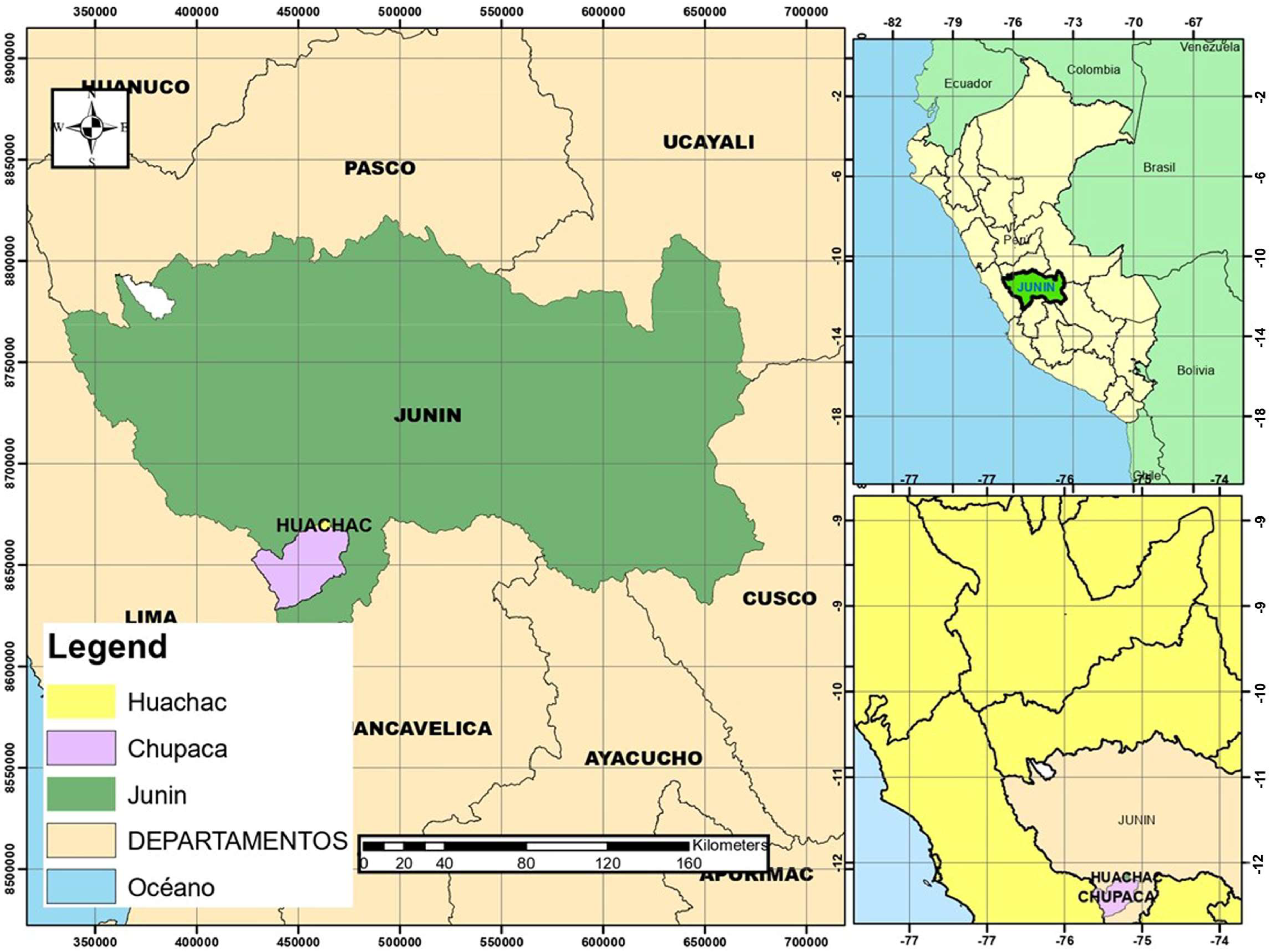
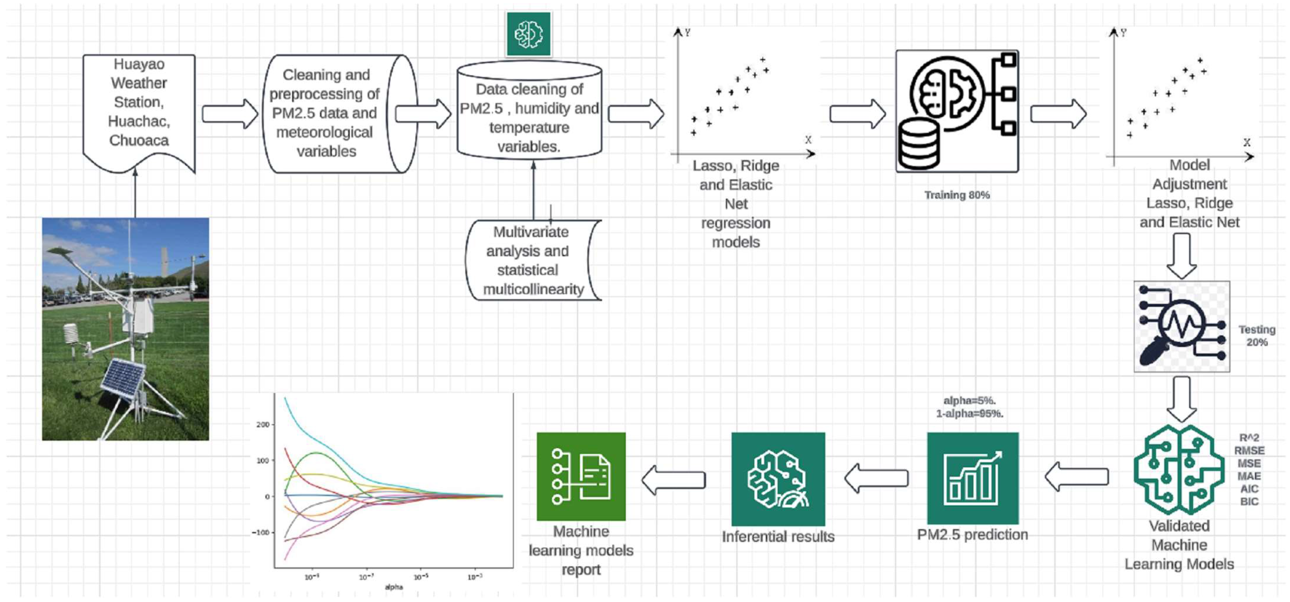
This study was conducted in the district of Huachac, province of Chupaca, department of Junín, Peru, where data were collected from the HUAYAO monitoring station using geolocation tools and software with Python 3.11 libraries. A sample of 16,543 records was conditioned and normalized using the EDA methodology.

The problem is atmospheric pollution by particulate matter in the environment, and this article aims to predict the behavior of PM_2.5 particulate matter, applying machine learning methodology in order to make decisions for the benefit of the surrounding population.

This study provides a predictive machine learning model of PM2.5, which contributes to the predictive understanding of the behavior of environmental variables in the study areas, which will allow international bodies to use it as a model for analysis.

2. Materials and Methods

2.1. Study Area

This study was conducted in the district of Huachac, province of Chupaca, department of Junín, Peru, located at 3275 masl and 290 km from the capital of the country (Lima), 22 km northwest of Huancayo, bordering to the north with the district of Manzanares, to the south with the city of Chupaca, to the east with the district of Sicaya and to the west with the district of Chambara in the province of Concepción, as shown in Figure 1. The data were obtained from the HUAYAO monitoring station, which is located in the district of Huachac, province of Chupaca, department of Junín, Peru.

2.2. Research Method

The research method is presented in Figure 2, in which data were collected from the Huayao, Junin, Peru station, then an exploratory analysis of the collected data (EDA) was performed, imputing outliers and cleaning data justifying the prerequisites of normality, linearity and homoscedasticity [21]. Then, the machine learning models lasso, ridge, and elastic net were applied to determine which one was the most optimal.

2.2.1. Machine Learning Models

Machine learning, a branch of AI, develops algorithms and models to enable computers to learn and make data-driven decisions without explicit programming, fostering autonomous and efficient machine learning [22]. ML and statistics are closely related, with ML relying on many statistical principles and methods [23].

Linear regression is an extension of the population regression model (PRF) with k variables, where the dependent variable is Y, and the k − 1 explanatory variables are $X_2, X_3, X_4, X_5, \cdots , X_k$ [24,25], as shown in Equation (1).

$$Y_i={\beta }_1+{\beta }_2{X}_{2i}+{\beta }_3{X}_{3i}+{\beta }_4{X}_{4i}+\cdots +{\beta }_k{X}_{ki}+u_i; i=1,\cdots ,n$$

(1)

where ${\beta }_1$ is the intercept, ${\beta }_2$ to ${\beta }_k$ are the partial slope coefficients, $u$ is the stochastic disturbance term, and i is the i-th observation, with n as the population size. Equation (1) is a shorthand expression for the set of n simultaneous equations [26,27].

LASSO (Least Absolute Shrinkage and Selection Operator) regression is a regression method used for variable selection and regularization in linear regression methods. Its main objective is to reduce the complexity of the model by penalizing the coefficients of the least important variables, bringing them to zero [28]. The LASSO regression method is used for the selection of variables and regularization in linear regression methods.

According to Qian, P [29], LASSO (Least Absolute Shrinkage and Selection Operator) regression is a regularization technique for variable selection and model complexity reduction in machine learning and statistics. It is an extension of linear regression with a penalty to avoid overfitting [30]. LASSO is used when there are many features, helping in variable selection while fitting a predictive model [31]. The LASSO loss function combines the linear regression loss (mean squared error) and the absolute value of feature coefficients multiplied by a hyperparameter λ [32].

LASSO regression is a restricted method since it selects the influential variables in a variable called response, resulting in zero coefficients. Through this procedure, a strong set of instruments is sought, which provides the greatest amount of information about the endogenous variables in the first stage of estimation [29].

The LASSO regression model is mathematically represented by Equation (2), which aims to minimize the parameters α in the errors by taking the penalty of the model coefficients [25,33].

$$\underset{\alpha ,\beta }{Minimize}\left\{{\displaystyle \frac{1}{2n}}\sum _{i=1}^N{\left(y_i-\alpha -\sum _{j=1}^p{x}_{ij}{\beta }_j\right)}^2\right\}$$

(2)

In performing the Lasso regression, we add a penalty factor to the least squares, which reduces the loss function S to a minimum value, represented by Equations (3) and (4).

$$S=\underset{\alpha ,{\beta }_1,{\beta }_2}{\mathit{Min}}\left[u_i^2+\lambda \left(\left|{\beta }_1\right|+\left|{\beta }_2\right|\right)\right]$$

(3)

$$S=\underset{\alpha ,{\beta }_1,{\beta }_2,{\beta }_3,{{\beta }_4,\beta }_5}{\mathit{Min}}\left[{\left(Y_i-\alpha -{\beta }_1{X}_{i1}-{\beta }_2{X}_{i2}\right)}^2+\lambda \left(\left|{\beta }_1\right|+\left|{\beta }_2\right|\right)\right]$$

(4)

The RIDGE model penalty is appropriate in the case where there are multiple predictors, and they are drawn from a Gaussian distribution [34]. The mean squared error of Ridge regression involves the variance and bias of the estimator; the theorem on the mean squared error function is very important for its analysis [35]. The Ridge regression model is given in Equation (5).

$${\beta }^{ridge}=\underset{\beta ϵ\mathbb{R}}{\mathit{argmin}}{‖Y-X\beta ‖}_2^2+\lambda {‖\beta ‖}_2^2$$

(5)

The elastic net regression penalty is an adaptation of least squares and allows addressing the estimation problem by producing a biased β estimator but with small variances [21,25,32]. The mathematical representation of the elastic net regression model is represented in Equation (6), defined as follows:

$${\beta }^{EN}=\underset{\beta ϵ\mathbb{R}}{\mathit{argmin}}{{\displaystyle \frac{1}{2n}}‖Y-X\beta ‖}_2^2+\lambda \left[{\left(1-\alpha \right)‖\beta ‖}_2^2+\alpha {‖\beta ‖}_1\right]$$

(6)

2.2.2. Metrics for Validation of Predictive Models

Exploratory data analysis (EDA), allows a clear view of the data, performing descriptive analysis, adjustment of variable types, detection and treatment of missing data, identification of outliers and correlation of variables [36]. In descriptive analysis, one dives into the data to understand its structure and nature. This includes generating summary statistics, such as mean, median, standard deviation, and creating graphs that reveal the distribution of the data. This is followed by adjusting the types of variables in which the data can be presented in different formats and types (numerical, categorical, dates, etc.) [37]. In this phase, the variables are adjusted and transformed as necessary to ensure that they can be used effectively in the analysis. In addition, missing data are detected and processed, where incomplete data can be a challenge. During EDA, we identified observations with missing data and considered options such as imputation or deletion of rows or columns to ensure completeness of results, as well as identified outliers, known as outliers. The EDA helped us to identify and understand these values to determine if they should be treated or if they are legitimate and significant. Finally, correlation of variables was performed to explore the relationships between variables, using statistical techniques and visualizations to discover connections and patterns that can reveal valuable information about the particulate matter problem analyzed in the research [13,38].

Metrics used in this study [22] include the MAE, which measures the average magnitude of the errors in the predictions and is shown in Equation (7) [39,40].

$$Mean Absolute Error: MAE={\displaystyle \frac{1}{n}} {\sum }_{i=1}^n\left|y_i-\widehat{y_i}\right|$$

(7)

Likewise, the RMSE (root mean squared error) is the square root of the average of the squared differences between the prediction and the actual observation (SSE/n) and is defined by Equation (8).

$$Root Mean Square Error: RMSE=\sqrt{{\displaystyle \frac{1}{n}}{\sum }_{i=1}^n{\left(y_i-\widehat{y_i}\right)}^2}$$

(8)

The coefficient of determination $R^2$ measures the variance in the data explained by the model and determines the relationship between the sum of the squares of the errors and the total shown in Equation (9) [41,42].

$$Coefficient of determination:{\mathrm{R}}^2=1-{\displaystyle \frac{{\sum }_{\mathrm{i}=1}^{\mathrm{n}}{\left({\mathrm{y}}_{\mathrm{i}}-\widehat{{\mathrm{y}}_{\mathrm{i}}}\right)}^2}{{\sum }_{\mathrm{i}=1}^{\mathrm{n}}{\left({\mathrm{y}}_{\mathrm{i}}-\overline{{\mathrm{y}}_{\mathrm{i}}}\right)}^2}}$$

(9)

Based on existing knowledge, the model that typically demonstrates the best efficiency in predicting PM_2.5AQI is often determined through comparative analysis of various regression techniques, such as ridge, lasso, and elastic net regression. The key factors influencing model efficiency are as follows [43]:

• Model Selection: the choice between ridge, lasso, and elastic net can impact performance based on the nature of the dataset.
• Penalty Values: adjusting penalty values can optimize each model’s ability to prevent overfitting or underfitting.
• Feature Selection: models like lasso are particularly effective at feature selection, which can enhance predictive accuracy.
• Cross-Validation: techniques like k-fold cross-validation help in assessing model performance more reliably.

In fact, to determine the best-performing model for PM_2.5AQI prediction, one would typically analyze metrics such as mean absolute error (MAE), root mean square error (RMSE), and R-squared values across different models and configurations. The model yielding the lowest error metrics and highest R-squared value would be considered the most efficient for this specific prediction task [42,44,45,46].

3. Results

A total of 16,543 records were analyzed for the variables under study, as shown in

Table 1. Description of the study variables.

Title 1	Media	DE
PM2.5AQI	33.1	2.75
Humidity	4.72	0.987
Temperature	10.8	0.23

, where PM_2.5AQI shows a data density with a trend to the left and a tail to the right due to the outliers on some days of the year but in general shows a mean of 33.1, with a standard deviation of PM_2.5 and a maximum value of 208, which represents an outlier and poses a risk to the health of the population. Absolute humidity showed a normal distribution since it had a mean of 4.72% with a median of 4.8 and a standard deviation of 0.987, indicating a relatively stable humidity over time. Likewise, the temperature showed an average of 10.8 °C with a median of 9 and a standard deviation of 0.23, with a temperature ranging between −6 and 28.

Figure 3 shows the PM_2.5AQI, with the highest concentration in winter with an average of 52.6 g/m³, in second place in spring with an average of 36.9 g/m³, in third place in autumn with an average of 27.4 g/m³ and finally in summer with an average of 15.6 g/m³.

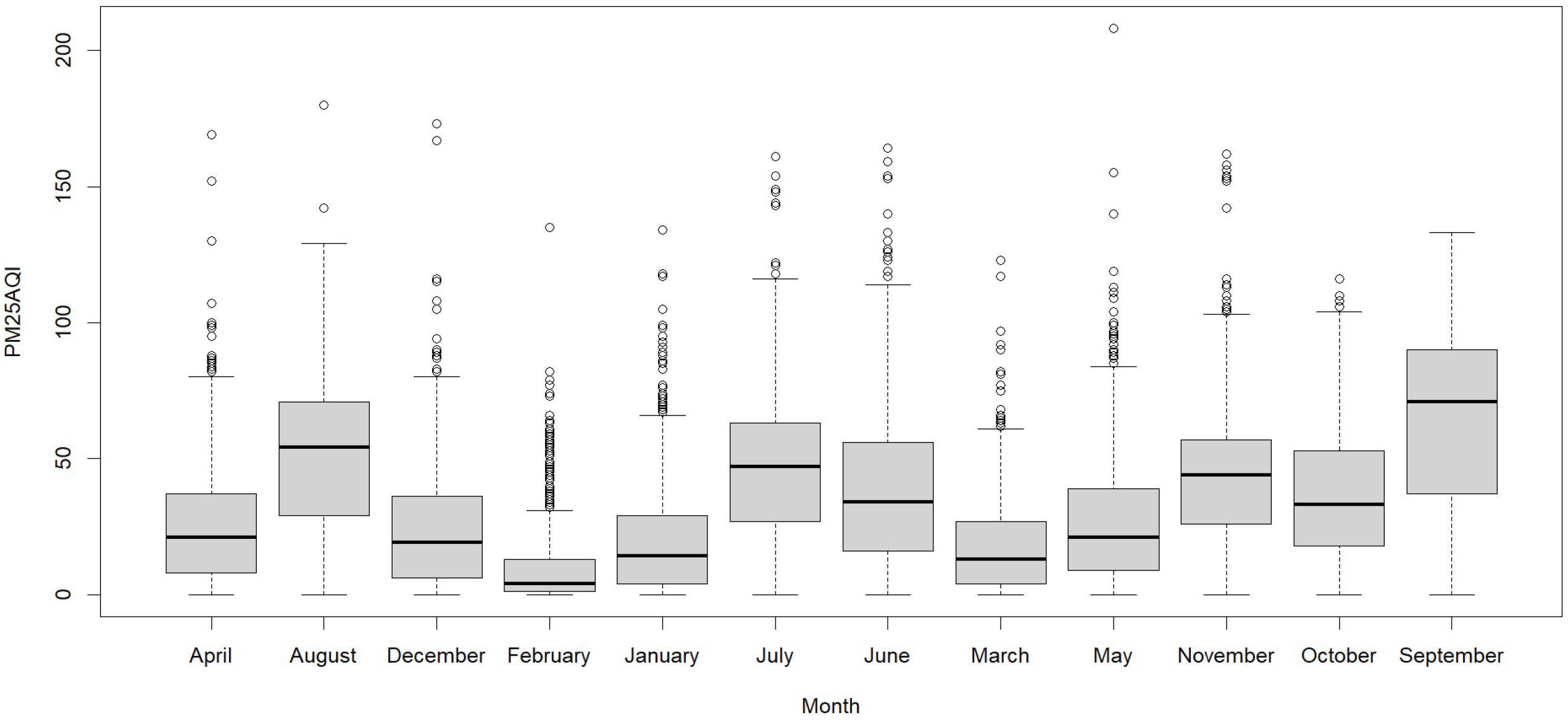
In Figure 4, we observe the PM_2.5AQI by month for the year analyzed. In September, the index was 64.9, followed by August in second place with 51.7, July in third place with 46.0, and November in fourth place with 43.10. The remaining months had indices lower than 38.7.

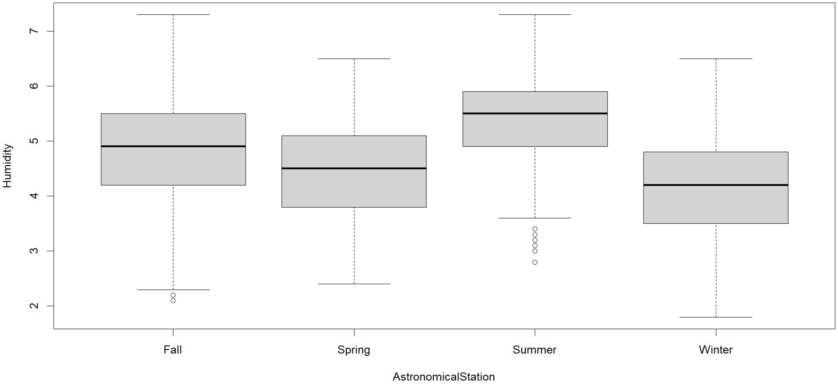
In Figure 5, we observe that in summer, 50% have a humidity lower than 5.5, and the other 50% have a humidity higher than 5.5; secondly, in autumn, 50% have a humidity lower than 4.9, and the other 50% have a humidity higher than 4.9; thirdly, in spring, 50% have a humidity lower than 4.5, and the other 50% have a humidity higher than 4.5; and finally, in spring, 50% have a humidity lower than 4.2, and the other 50% have a humidity higher than 4.

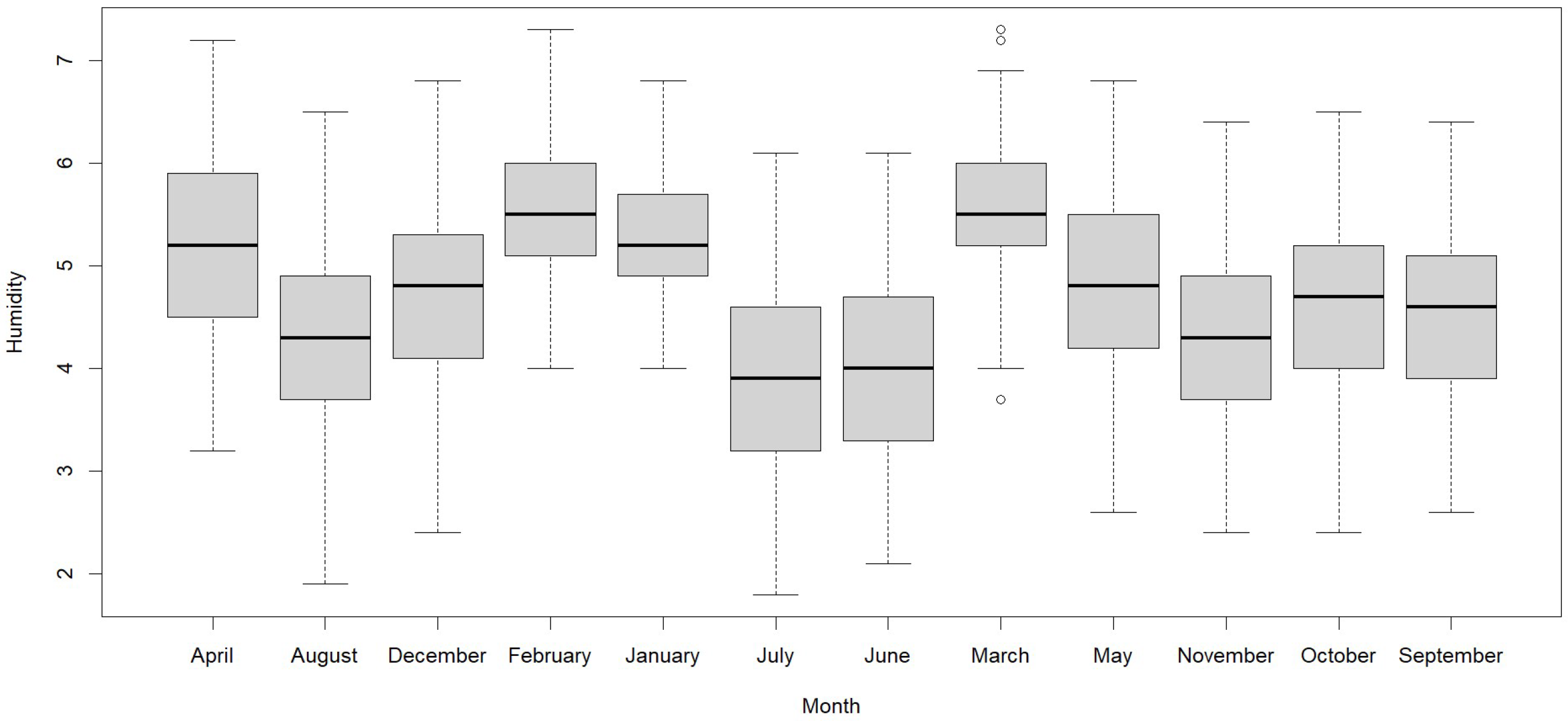
Humidity shows its highest value in January due to heavy rains and its lowest value in July due to the dry season of the year and the frost season. The absolute humidity shows that it is higher in summer, followed by autumn, due to the beginning and end of the rain. In Figure 6, we observe that in February and March, 50% have a humidity lower than 5.5, and the other 50% have a humidity higher than 5.5. In second place, in January and April, 50% have a humidity lower than 5.2, and the other 50% have a humidity higher than 5.2. In third place, in May and December, 50% have a humidity lower than 5.2, and the other 50% have a humidity higher than 5.2.2. Thirdly, in May and December, 50% have a humidity lower than 4.8, and the other 50% have a humidity higher than 4.8. In October, 50% have a humidity lower than 4.7, and the other 50% have a humidity higher than 4.7. Finally, in the other months, 50% have a humidity lower than 4.6, and the other 50% have a humidity higher than 4.6.

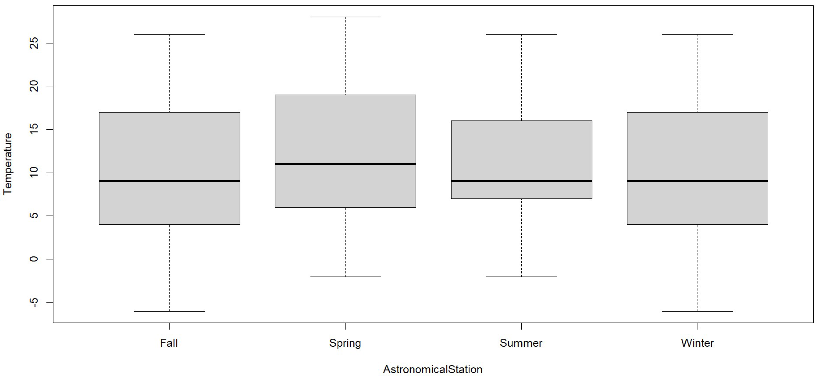
In Figure 7, we observe that in spring, 50% have a temperature lower than 11 °C and the other 50% have a temperature higher than 11 °C, and there is a temperature tie in autumn, winter, and summer, with 50% having a temperature lower than 9 °C and the other 50% having a temperature higher than 9 °C.

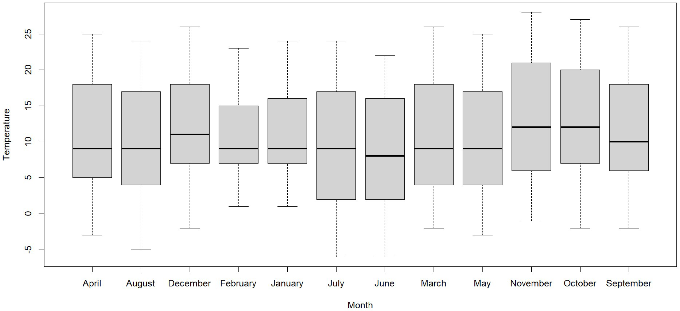
In Figure 8, we observe that in October and November, 50% have a temperature lower than 12 °C, and the other 50% have a humidity higher than 12 °C. Secondly, in December, 50% have a temperature lower than 11 °C, and the other 50% have a temperature higher than 11 °C. Thirdly, in September, 50% have a temperature lower than 10 °C, and the other 50% have a temperature higher than 10 °C. Finally, in the other months, 50% have a temperature lower than 9 °C, and the other 50% have a temperature higher than 9.

The temperature reaches its lowest value in June due to the presence of morning frosts and its highest point in November due to the sunny season. These values of the air quality index, humidity, and temperature are crucial for planning and decision making related to public health and the environment because, for example, the highest AQI indicates that the smoke of the entire Mantaro Valley, where the astronomical center of Huachac is located should make educational campaigns of not burning agricultural waste. The highest average temperature was in spring due to the absence of rain and wind in the area, and the lowest was in winter due to the presence of morning frosts. The standard deviation indicates that the variability is higher in winter compared to the other seasons because, in these months, there is the presence of low temperatures as the highest. The minimum and maximum values vary according to the season, with the highest and lowest values associated with winter and spring, although the highest is in autumn with an AQI of 208 due to the fact that farmers prepare their land for planting and burn crop stubble.

In the investigation of the 16,543 observations, 80% (13,234) of the observations were taken for training and 20% (3309) for testing. During training, a resampling cross-validation with three repetitions yielded an RMSE = 25.36203, an Rsquared = 0.1483206 and an MAE = 20.51858.

The multivariate linear regression analysis with two regressor variables (humidity and temperature), as well as the predictor variable PM_2.5AQI, fulfilled the statistical prerequisites and yielded the results in R Studio 2024.04.2 Build 764 software shown below.

>summary(lm)
Call:
lm(formula = .outcome ~ ., data = dat)
Residuals:
Min	1Q	Median	3Q	Max
−53.087	−19.664	−5.102	16.336	177.352
Coefficients:
	Estimate	Std. Error	t value	Pr(>|t|)
(Intercept)	83.40932	1.07213	77.798	<2 × 10−16 ***
Humidity	−10.37024	0.23201	−44.698	<2 × 10−16 ***
Temperature	−0.12717	0.03169	−4.013	6.04 × 10−5 ***
---
*** represents the significance of the results., signif. codes: 0 ‘***’ 0.001 ‘**’ 0.01 ‘*’ 0.05 ‘.’ 0.1 ‘ ’ 1
Residual standard error: 25.37 on 13,269 degrees of freedom
Multiple R-squared: 0.1478, Adjusted R-squared: 0.1477
F-statistic: 1151 on 2 and 13,269 DF, p-value: <2.2 × 10−16

In these results, the significance of the regressor variables was highly significant with a p-value less than $2\times {10}^{-16}$, allowing us to propose the multiple regression model for PM_2.5 shown in Equation (10).

$${PM}_{2.5}AQI=83.40932-10.37024\left(Humidity\right)-0.12717\left(Temperature\right)$$

(10)

This indicates that both humidity and temperature are inversely proportional with PM_2.5AQI for each unit increase in the predictor variables; in addition, the p-values in each of these variables are less than the significance level α = 0.05, which indicates that they have a significant effect and is corroborated by applying an analysis of variance of the model, also resulting in p-values less than α = 0.05 for both predictor variables. In addition, the Durbin–Watson test yields an autocorrelation of 0.881 and a DW of 0.238 with a p-value of less than α = 0.05, which indicates that there is almost no autocorrelation, which indicates the independence of the predictor variables, and all this is corroborated by the VIF of 1.08 for both variables, which indicates that both variables of the model are independent and there is no collinearity between them since it is very close to 1. Therefore, the model is found to be very predictively robust with a fairly high AIC of and BIC and with a low RMSE of 25.5 for the 16,544 data observed in the model with a p-value of less than 0.05.

Correlations of the predicted variable PM_2.5AQI with the predictor variables humidity and temperature were obtained. First, the correlation of PM_2.5AQI with humidity is −0.378, which shows a linear dependence and is inversely proportional, i.e., while PM_2.5AQI increases, absolute humidity decreases and vice versa, which means that the presence of humidity influences the decrease or increase in PM_2.5AQI present in the air. Likewise, we can see that the correlation between PM_2.5AQI and temperature has a correlation of −0.134, which indicates that it is also an inversely proportional correlation, which means that while PM_2.5AQI increases the temperature decreases, which gives us the idea that if the temperature increases, PM_2.5AQI decreases and also inversely, although this index shows that it is lower than the index presented by humidity, therefore it indicates that its linear influence on PM_2.5AQI is lower. 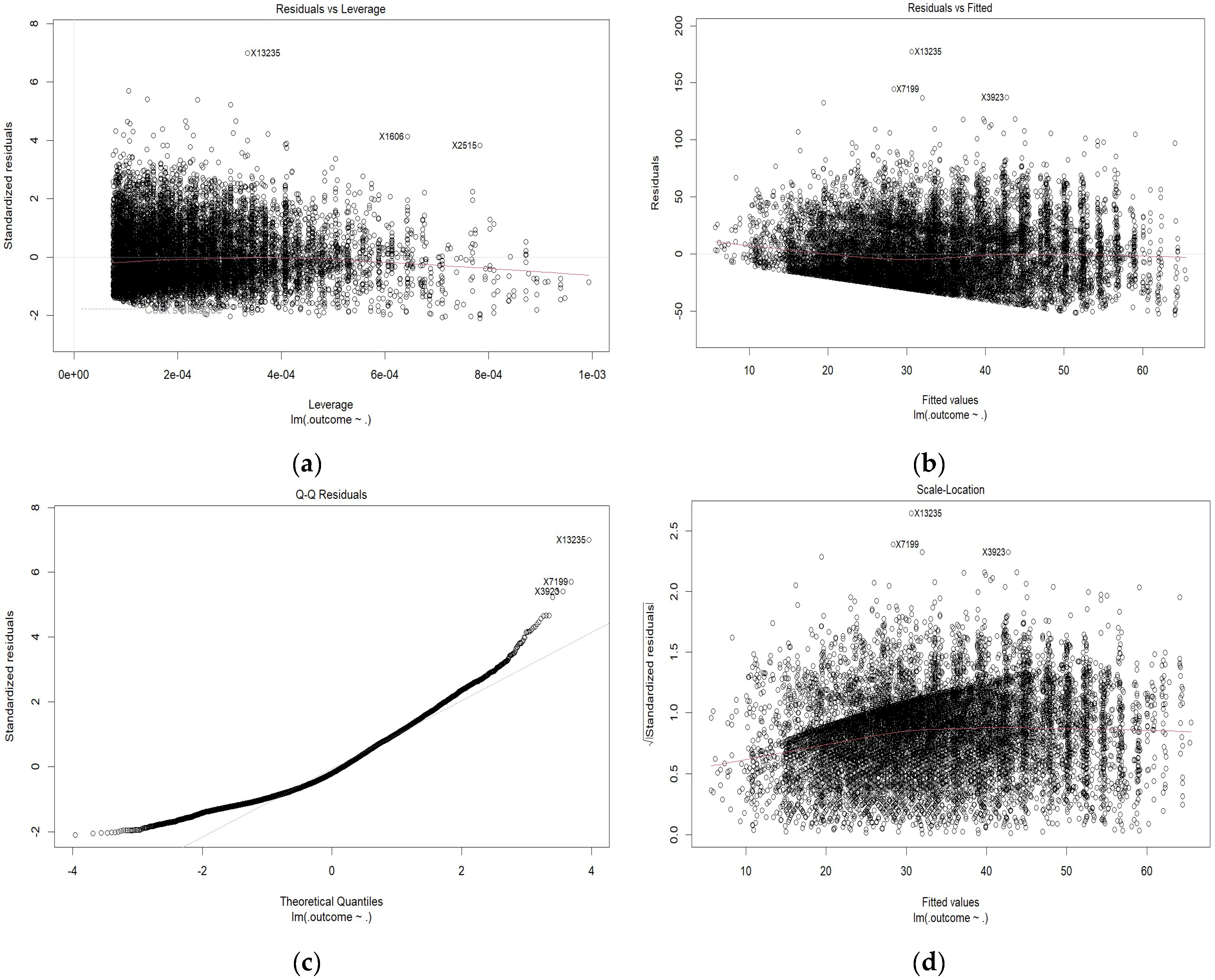On the other hand, the p-value for humidity and temperature is less than 0.05, which confirms the hypothesis that in both cases, there is a linear dependence between the predicted variable PM_2.5AQI and the predictor variables of humidity and temperature. The graphs shown in Figure 9 show the normalized residuals and fitted values, with residual quantiles and the root mean square error, for which the linear regression model meets all specifications and prerequisites for prediction.

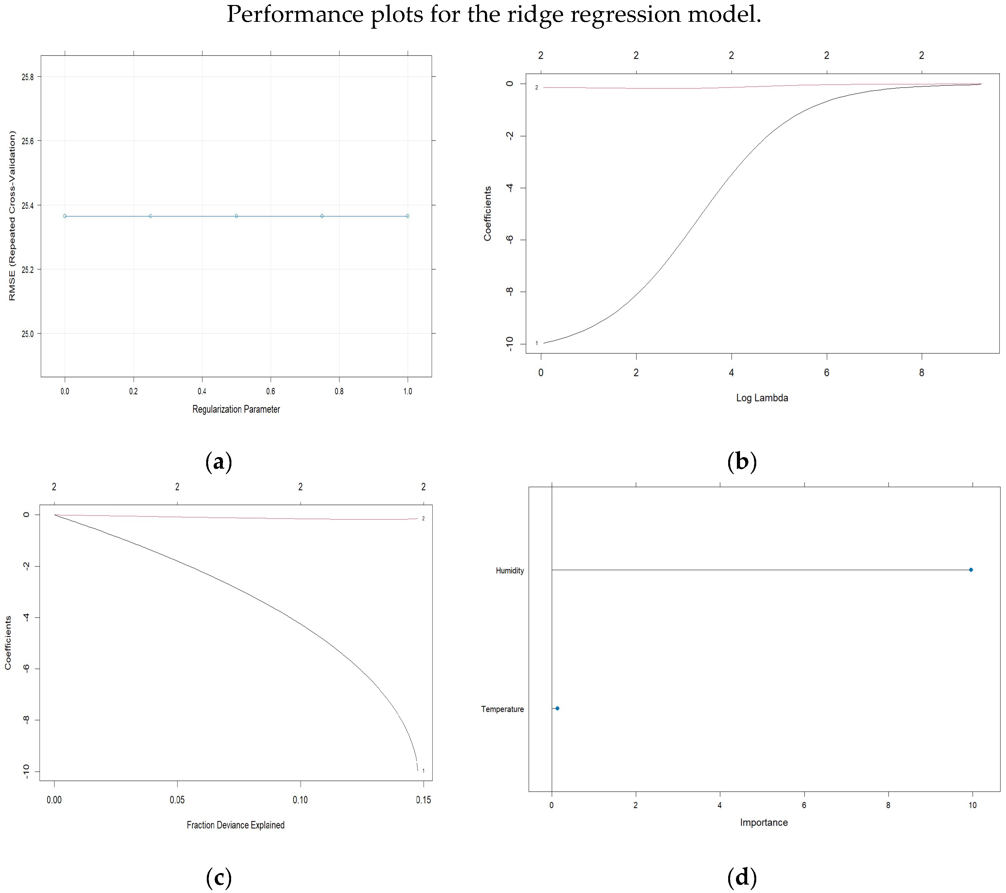
The results for the ridge regression model, with a training sample of 13,234 observations and a testing sample of 3309 observations, are presented in

Table 2. Performance metrics for the ridge regression model.

Lambda	RMSE	Rsquared	MAE
0.000100 *	25.36471	0.1483078	20.53783
0.250075	25.36471	0.1483078	20.53783
0.500050	25.36471	0.1483078	20.53783
0.750025	25.36471	0.1483078	20.53783
1.000000	25.36471	0.1483078	20.53783

* Penalty values $\lambda$ for the ridge model.

, which shows the resampling metrics across the fit parameters.

Figure 10 shows the plots for the ridge regression model with cross-validation and the logarithms of the Lambda penalty values, as well as the values of the model coefficients and the significance of the regressor variables.

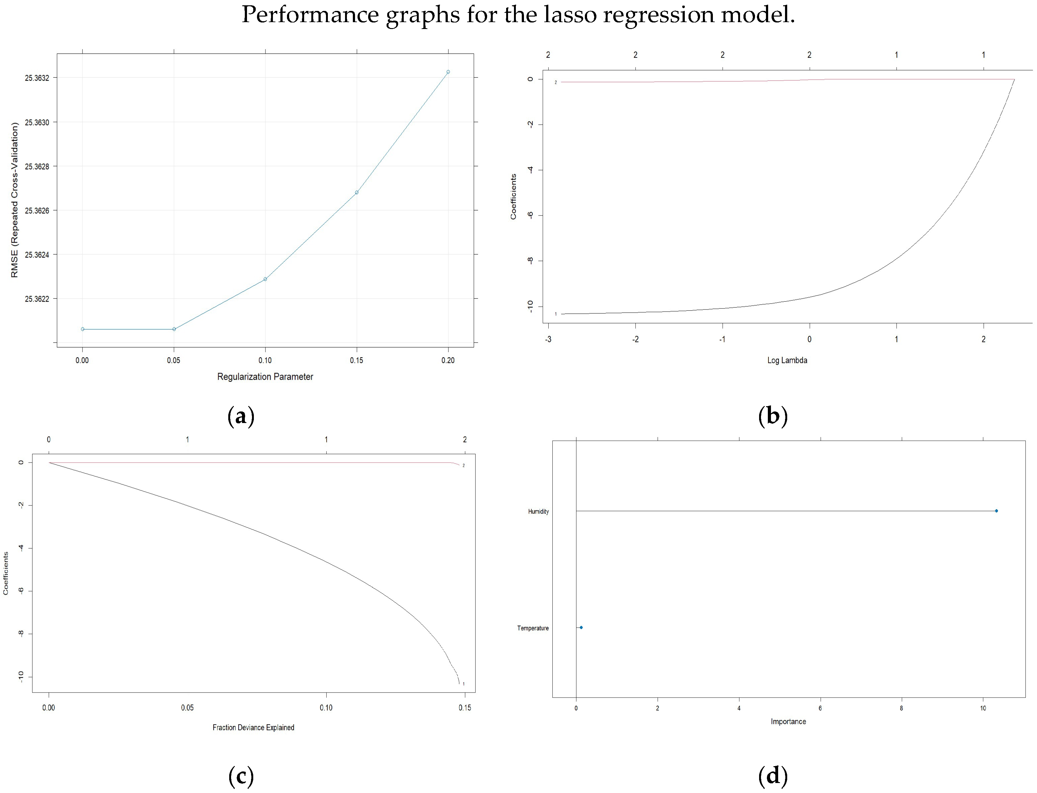
The results for the lasso regression model, with a training sample of 86,654 observations and a testing sample of 21,663 observations, are presented in

Table 3. Performance metrics for the lasso regression model.

Lambda	RMSE	Rsquared	MAE
0.000100 *	25.36206	0.1483177	20.51777
0.050075	25.36206	0.1483177	20.51777
0.100050	25.36229	0.1483129	20.52004
0.150025	25.36268	0.1483044	20.52282
0.200000	25.36323	0.1482928	20.52574

* Penalty values $\lambda$ for the lasso model.

, which shows the metrics obtained through resampling and the fit parameters.

Figure 11 shows the graphs for the lasso regression model with cross-validation and the logarithms of the Lambda penalty values, as well as the values of the model coefficients and the significance of the regressor variables.

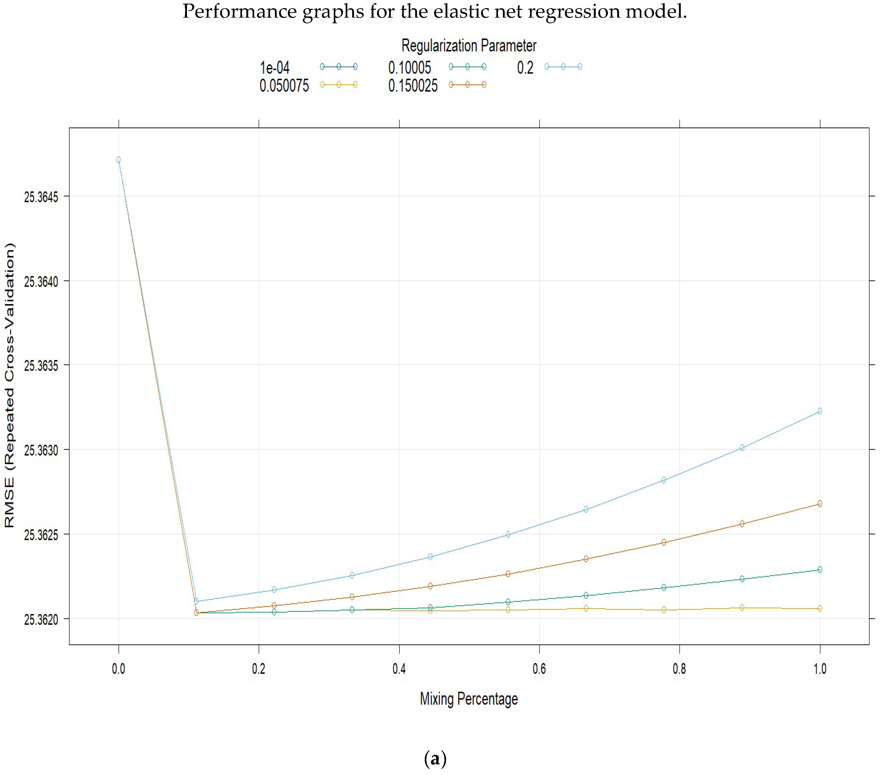
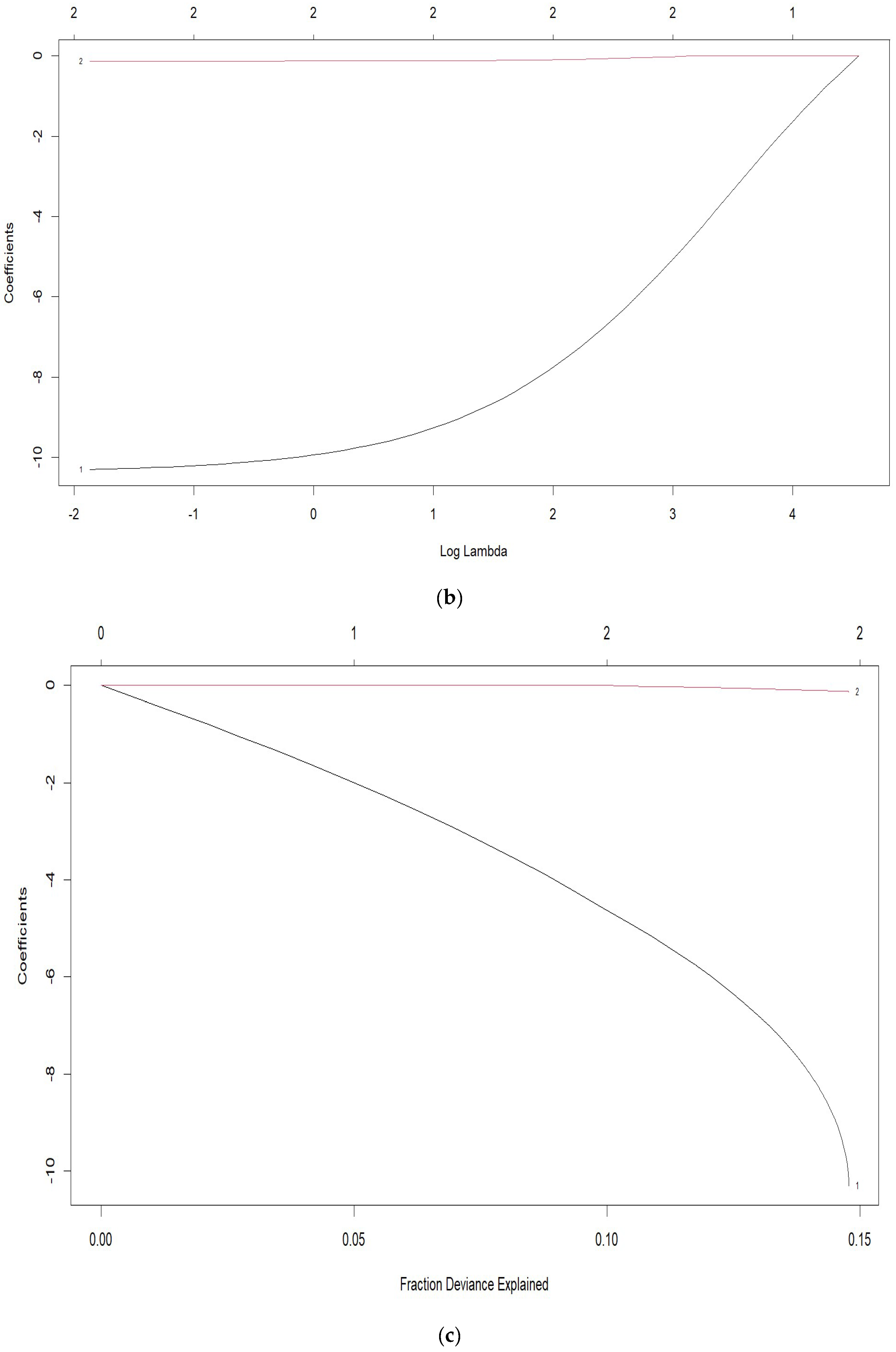
The results for the elastic net regression model, with a training sample of 13,234 observations and a testing sample of 3309 observations, are presented in

Table 4. Performance metrics for the elastic net regression model—MAE.

MAE	Min	Mean	Max
LinearModel *	19.72584	20.51489	21.24642
Ridge	19.75967	20.53783	21.24997
Lasso * Lasso * Lasso * Lasso * Lasso * Lasso * Lasso * Lasso * Lasso	19.73003	20.51777	21.24672
ElasticNet *	19.73139	20.51858	21.24663

* MAE metrics for predictive penalty models.

,

Table 5. Performance metrics for the elastic net regression model—RMSE.

RMSE	Min	Mean	Max
LinearModel *	24.33021	25.36196	26.30641
Ridge	24.33905	25.36471	26.28795
Lasso * Lasso * Lasso * Lasso * Lasso * Lasso * Lasso * Lasso * Lasso	24.33268	25.36206	26.30250
ElasticNet *	24.33179	25.36203	26.30244

* RMSE metric for the predictive penalty models.

and

Table 6. Performance metrics for the elastic net regression model—Rsquared.

Rsquared	Min	Mean	Max
LinearModel *	0.1035190	0.1483207	0.1794977
Ridge	0.1034498	0.1483078	0.1796028
Lasso * Lasso * Lasso * Lasso * Lasso * Lasso * Lasso * Lasso * Lasso	0.1035378	0.1483177	0.1794510
ElasticNet *	0.1035171	0.1483206	0.1795012

* Rsquared metrics for the predictive penalty models.

, which show the resampling metrics obtained through the fit parameters.

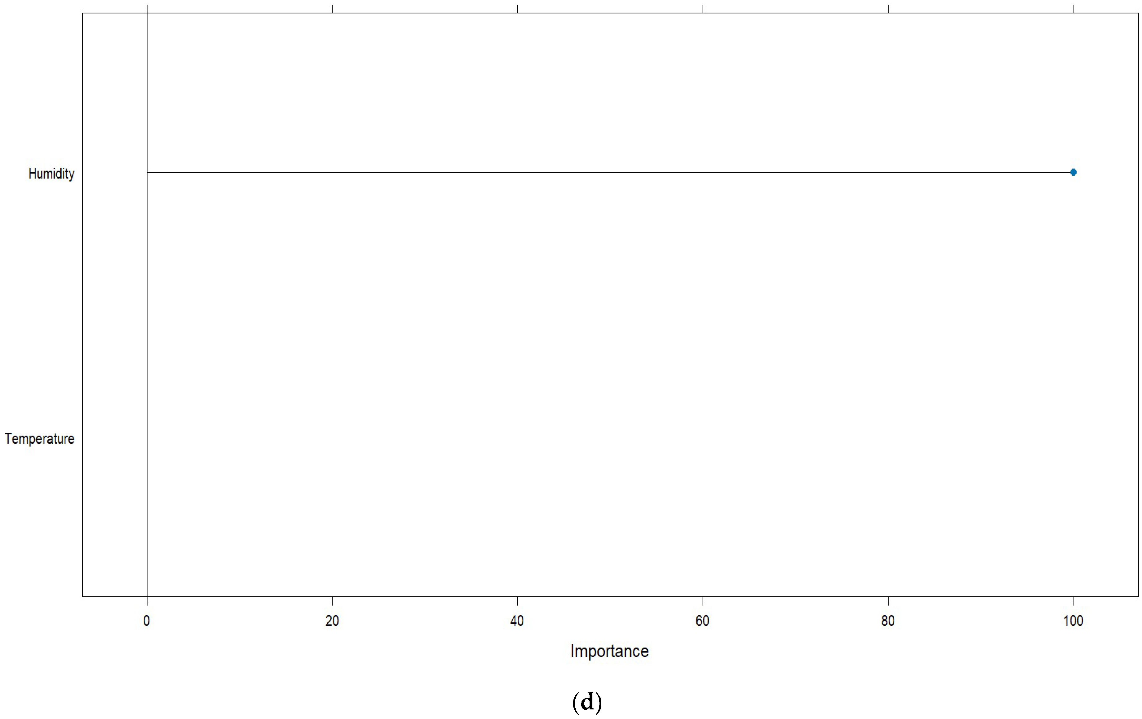
Figure 12 shows the graphs for the elastic net regression model with cross-validation and the logarithms of the Lambda penalty values, as well as the values of the model coefficients and the significance of the regressor variables.

The best model that allowed the prediction of PM_2.5AQI is the thirteenth one, with α = 0.1111111 and a Lambda of λ = 0.150025; the model is shown in Equation (11).

$${PM}_{2.5}AQI=83.0846522-10.3022000\left(Humidity\right)-0.1268124\left(Temperature\right)$$

(11)

This means that, for each year, the PM_2.5AQI decreases by 10.3022000; likewise, for temperature, the PM_2.5AQI decreases by 0.12688124. In the prediction for the mean squared error of the training set, a value of 25.36255 was obtained, and for the test set, a value of 25.84308 was obtained, resulting in a mean difference of 0.48053. This represents 98.1406% of the prediction efficiency with respect to the test.

4. Discussion

The LASSO (Least Absolute Shrinkage and Selection Operator) method applies regression procedures with parameter shrinkage to select predictor variables that matter significantly and mimic some variables that have little or no effect on the model by adjusting the maximum and minimum coefficients [24]. In the MLP and SVM modeling of Qian, they found RMSE values of 52.74 and 35.88, respectively; however, this research presents an RMSE of 25.5, which indicates a more optimal model, as it is much lower in fit value with the actual values recorded. This is in parallel with Juan Soria’s study [25], which presented a linear regression model for the prediction of PM2.5, finding a coefficient of 0.66105 μg/m³ and an intercept of 5.57229 μg/m³.

A linear regression model $y=60.219-1.7493x$ with a coefficient of determination $R^2=0.2836$ on the concentration of PM2.5 and PM10 in Lima and Callao using SENAMHI data [47], compared to the one found in this research of $R^2=$ 0.1478; likewise [27] found a linear regression equation between PM2.5 and PM10 in the industrial zone of the form y = 4.485924 + 0.567541x.

Geraldo-Campos et al. [31] found lasso and ridge regularization models for the prediction of credit risk in reactive Peru with 501,298 companies analyzed, economic sector, granting entity, amount covered, and department as regressors, and risk level as a predictor. They determined a lasso regression model with ${\lambda }_{60}=0.00038$ and an RMSE = 0.3573685, as well as a ridge regression model with ${\lambda }_{100}=0.00910$ and an RMSE = 0.3573812, represented in Equation (12).

$$\begin{array}{cc}\hfill Y_{Lasso}=0.51487& +0.05878\left(Economic sector\right)\hfill \\ & -0.19292\left(Credit granting entity\right)\\ & +1.29671\left(Amount covered\right)+0.03115\left(Departament\right)\end{array}$$

(12)

In this research, lasso (RMSE = 25.36206), ridge (RMSE = 25.36471), and elastic net (RMSE = 25.36203) models were found, where the best model found with an α = 0.1111111 and a Lambda value λ = 0.150025 is represented in Equation (13). Then, the choice of penalty values in regression models is crucial for achieving optimal performance by managing the trade-off between bias and variance, influencing both model complexity and predictive power [48,49].

$$Y=83.0846522-10.3022000\left(Humidity\right)-0.1268124\left(Temperature\right)$$

(13)

This is further contrasted with Equation (13), finding the elastic net predictive regression model shown in Equation (14), which was used to predict teacher salary with α = 0.5555556, a Lambda λ = 0.2, and an RMSE of 895.3383.

$$\begin{array}{cc}\hfill Y=-3092.582975& -4.824496\left(Edad\right)+22.972778\left(NEduc\right)\hfill \\ & +17.623234\left(TServ\right)-88.511756\left(EsDoc\right)\\ & +191.104877\left(HoLab\right)\end{array}$$

(14)

Overall, the data reveal interesting patterns about the seasons of the year and their impact on air quality, humidity, and temperature. These findings could be useful to better understand how these variables change throughout the year and how they could affect people who are quite vulnerable to the environment around them because having polluted air can even be deadly in some cases [50]. The research found that the increase in air quality in summer could have positive implications for public health in the central highlands, while the higher humidity in spring and summer could influence the comfort and well-being of people since these are times when most of the experiential tourism is generated in this area. Seasonal variability in temperature could also have consequences in various areas, from agriculture to the generation of the economy [47].

Analysis of the data provided reveals significant differences between seasons in terms of air quality, humidity, and temperature. These findings could be important to better understand seasonal patterns in these variables and their potential impacts on society and the environment. The paper highlights the importance of considering seasonal variations when addressing air quality and climate issues and suggests further research to fully understand the implications of these findings.

PM2.5AQI values show significant variations throughout the year, with a peak in September due to the constant burning of stubble [51] and agricultural waste by farmers prior to the annual planting of their products, which is detrimental to air quality. This merits a call to the local authorities to carry out environmental education campaigns because the presence of PM2.5 in the air often has fatal consequences, especially in vulnerable [46]. Humidity and temperature also show interesting fluctuations during the months of the year, with humidity presenting higher values in January due to the presence of heavy and intense rains in the central highlands of Peru, [50] which makes absolute humidity more concentrated at this time. The lowest temperature recorded in June was −6 °C, and the maximum reached 22 °C, showing significant variability in temperature due to the presence of morning frosts, according to the findings of Saavedra et al. [49]. The data presented are within the ranges found by other researchers in terms of monthly variations in air quality, humidity, and temperature.

5. Conclusions

The best predictive model found is quite robust given that it meets the indicators in favor of the model LASSO regression analysis with a high AIC and BIC and a low RMSE for the 16,543 data analyzed. This is the thirteenth model, which emerged as the best predictor for the PM_2.5 air quality index (AQI) with specific parameters: Alpha: 0.1111111 and Lambda: 0.150025. The model predicts a decrease in PM_2.5AQI by 10.3022000 units per year, for temperature changes, PM_2.5AQI decreases by 0.12688124 units, the mean squared error (MSE) for training is 25.36255, while for testing it is 25.84308, resulting in a mean difference of 0.48053, this indicates an impressive prediction efficiency of 98.1406% when comparing training to testing outcomes. These results highlight the effectiveness of regression models in predicting PM_2.5AQI and provide a basis for future analysis and refinement of predictive techniques for management and planning of air quality improvement by government authorities in the Mantaro Valley.

The season with the highest PM_2.5AQI was winter, with a value of 52.6 with a variability of 29.4, which is less than 100, indicating “Moderate” or there may be moderate health problems for people who are unusually sensitive to air pollution.

PM_2.5AQI shows a peak in September due to smoke from stubble burning by farmers, while humidity peaks in January due to rainfall during that season and the minimum temperature in June due to the presence of frost.

These data are vital for understanding seasonal fluctuations in these environmental parameters, which have important implications for public health and environmental planning. The data found show that in general most of the year presents good air quality, showing some peaks of unsatisfactory AQI (208) as discordant or anomalous.

In conclusion, an efficient machine learning predictive model was obtained for the prediction of PM2.5AQI, which allows the measurement of future air quality and enables decision making in environmental care.

According to the monitoring protocol of the Ministry of Environment of Peru (MINAM), the number of monitoring stations should be proportional to the size of the population; to overcome this limitation, a greater number of monitoring stations should be considered in future research.