Microphysical Characteristics of a Sea Fog Event with Precipitation Along the West Coast of the Yellow Sea in Summer

Abstract

The microphysics and visibility (Vis) of a sea fog event with precipitation were measured at the Baguan Hill Meteorological Station (BGMS) (36.07° N, 120.33° E; 86 m above sea level) from 27 June to 28 June 2022. The duration of the fog process was 880 min. The mean value of the number concentration (N_d) was 190.62 cm⁻³, and the mean value of the liquid water content (LWC) was 0.026 g m⁻³. Small droplets contributed 81% to N_d and had a greater impact on visibility attenuation, while larger droplets accounted for 58% of the total LWC. The observed droplet size distribution (DSD) was better represented by the G-exponential distribution than by the Gamma distribution. Incorporating both N_d and LWC in Vis parameterization resulted in the best prediction performance. This work enhances understanding of sea fog microphysics in the west coast of Yellow Sea in summer and highlights the need for long-term observations.

1. Introduction

Sea fog occurs in the lower atmosphere over oceans, coastlines, and islands, characterized by a significant reduction in visibility (Vis) due to the condensation of water vapor [1]. Coastal fog is considered a subtype of sea fog [2]. When the sea fog moves in, Vis drops to below 1 km, and in some cases, to just a few dozen meters. This can severely impact aviation, transportation, and human activities along the coastal areas, classifying it as a hazardous weather phenomenon [3,4,5]. Therefore, improving the accuracy of forecasts is essential to reduce economic losses and protect lives during fog events.

Fog significantly affects Vis, primarily due to its microphysical characteristics, such as number concentration (N_d), liquid water content (LWC), effective radius (r_e), mean radius (r_m), and droplet size distribution (DSD) [2,6]. Accurate prediction of Vis requires a thorough understanding of these features. However, current models often struggle to provide precise predictions, typically treating N_d as a constant or assuming a specific DSD [7,8]. To improve forecast accuracy, numerous field observation projects have been conducted worldwide to develop Vis parameterization schemes [4,9,10].

The Yellow Sea, particularly its western coast near Qingdao, is one of China’s most fog-prone regions, with frequent sea fog events occurring from April to July [11]. Despite this, recent studies on the microphysical characteristics of coastal fog near Qingdao are scarce. Wang et al. [12] documented a spring 2017 sea fog event at the Qingdao Meteorological Station (QDMS), analyzing its microphysical properties and introducing a new distribution function for fog DSD. In this study, we examined a sea fog event with precipitation from 27 to 28 June 2022, analyzing its microphysical characteristics to further understand coastal fog properties in Qingdao.

The rest of the paper is organized as follows: Section 2 describes data and methods. Section 3 presents the results of the microphysical characteristics and the suitable expression for DSD. Finally, we compare various parameterization schemes for calculating Vis of this fog process. Section 4 gives the summary and conclusions.

2. Materials and Methods

2.1. Study Location and Instrumentation

The study site is located at Baguan Hill Meteorological Station (BGMS) in the Ocean University of China, Shandong Province, China (36.07° N, 120.33° E; 86 m above sea level). BGMS is about 600 m from the sea, closer to the shore than QDMS where Wang et al. conducted their study [12] (Figure 1). Climatic data indicate that southeast winds prevail in the Qingdao area during sea fog events, transporting warm, humid air from the Yellow Sea to the coast and providing sufficient water vapor for fog formation. The absence of buildings in this direction makes it suitable for long-term sea fog observations.

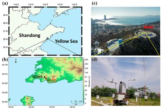
Figure 1. (a) Map of Shandong Province, China, adjacent to the Yellow Sea. (b) Locations of QDMS (black triangle) and BGMS (red circle), along with the surrounding topography. The color shading represents the elevation of the terrain. (c) Photograph of the BGMS observation site and (d) the instrument setup.

For this study, we used a Droplet Measurement Technology Fog Monitor (FM-120) (Longmont, CO, USA) and an automatic meteorological station at BGMS. The FM-120 enables continuous measurement of microphysical quantities, including N_d, LWC, and particle number concentrations across different diameters. Particle diameters range from 2 to 50 μm, divided into 30 bins, with a sampling frequency of 1 Hz. The automatic meteorological station collects data on Vis, air temperature (Ta), relative humidity (RH), precipitation, surface wind, and other parameters every minute.

Previous studies identified droplet loss as a key source of uncertainty in FM-120 [13]. This issue is particularly significant in ship-based observations, where ship speed and wind speed can push or pull the sampled air, creating turbulent pulsations at the FM-120’s inlet, leading to data bias that requires correction [14]. However, recent studies showed that aligning the spectrometer inlet with the prevailing wind direction on land minimized particle loss and size discrepancies, eliminating the need for data correction [15,16]. To ensure data quality, the instrument was rigorously calibrated before use. We also aligned the spectrometer inlet with the climatological prevailing wind direction (southeast) in Qingdao’s coastal area to reduce measurement errors.

2.2. Calculation Methods

The microphysical parameters can be calculated as follows:

$${\mathrm{N}}_{\mathrm{d}}=\int \mathrm{n}\left(\mathrm{r}\right)\mathrm{d}\mathrm{r},$$

(1)

$$\mathrm{L}\mathrm{W}\mathrm{C}=\int {\displaystyle \frac{4}{3}}\mathsf{\pi }{\mathsf{\rho }}_{\mathrm{w}}\mathrm{n}\left(\mathrm{r}\right){\mathrm{r}}^3\mathrm{d}\mathrm{r},$$

(2)

$${\mathrm{r}}_{\mathrm{m}}={\displaystyle \frac{\int \mathrm{n}\left(\mathrm{r}\right)\mathrm{r}\mathrm{d}\mathrm{r}}{\int \mathrm{n}\left(\mathrm{r}\right)\mathrm{d}\mathrm{r}}},$$

(3)

$${\mathrm{r}}_{\mathrm{e}}={\displaystyle \frac{\int \mathrm{n}\left(\mathrm{r}\right){\mathrm{r}}^3\mathrm{d}\mathrm{r}}{\int \mathrm{n}\left(\mathrm{r}\right){\mathrm{r}}^2\mathrm{d}\mathrm{r}}},$$

(4)

where n(r) is the number concentration of droplets at each bin interval, r is the midpoint radius of each bin, and ρ_w is the density of water (10⁻⁶ g m⁻³).

Equations (3) and (4) reference two parameters that describe particle size: r_m, the statistical mean radius, and r_e, the effective radius, which is widely regarded as the optimal parameter for characterizing scattered light and assessing the impact of cloud droplets on cloud albedo [17,18].

According to the Koschmieder formula [19], Vis is defined as:

$$\mathrm{V}\mathrm{i}\mathrm{s}=-\mathrm{l}\mathrm{n}\left(\mathsf{\epsilon }\right)/{\mathsf{\beta }}_{\mathrm{e}\mathrm{x}\mathrm{t}},$$

(5)

where ε is the brightness contrast threshold which is assumed to be 0.02 [20,21]. Vis sensor extinction coefficient (β_ext) is the sum of the extinction coefficient of fog droplets, which can be calculated by Mie theory [22]. Then, the value of Vis is clear. The detailed calculation process can be referred to [12].

In the evaluation of the estimated model performance, the following metrics can be used:

$$\mathrm{S}\mathrm{S}\mathrm{T}=\sum _{\mathrm{i}=1}^{\mathrm{k}}{\left({\mathrm{y}}_{\mathrm{i}}-\overline{\mathrm{y}}\right)}^2,$$

(6)

$$\mathrm{S}\mathrm{S}\mathrm{E}=\sum _{\mathrm{i}=1}^{\mathrm{k}}{\left({\mathrm{y}}_{\mathrm{i}}-{\widehat{\mathrm{y}}}_{\mathrm{i}}\right)}^2,$$

(7)

$${\mathrm{R}}^2=1-{\displaystyle \frac{\mathrm{S}\mathrm{S}\mathrm{E}}{\mathrm{S}\mathrm{S}\mathrm{T}}},$$

(8)

$$\mathrm{M}\mathrm{A}\mathrm{E}={\displaystyle \frac{1}{\mathrm{k}}}\sum _{\mathrm{i}=1}^{\mathrm{k}}|{\mathrm{y}}_{\mathrm{i}}-{\widehat{\mathrm{y}}}_{\mathrm{i}}|,$$

(9)

$$\mathrm{R}\mathrm{M}\mathrm{S}\mathrm{E}=\sqrt{{\displaystyle \frac{1}{\mathrm{k}}}\sum _{\mathrm{i}=1}^{\mathrm{k}}{\left({\mathrm{y}}_{\mathrm{i}}-{\widehat{\mathrm{y}}}_{\mathrm{i}}\right)}^2},$$

(10)

where ${\mathrm{y}}_{\mathrm{i}}$ represents the observed values, ${\widehat{\mathrm{y}}}_{\mathrm{i}}$ represents the estimated values, and $\overline{\mathrm{y}}$ is the mean. SST denotes the total sum of squares, SSE represents the sum of squared errors, R² is the coefficient of determination, MAE is the mean absolute error, and RMSE is the root mean square error. Lower values of SST, SSE, MAE, and RMSE indicate a smaller discrepancy between fitted and observed values, while an R² value closer to 1 signifies a better fit [23,24].

3. Results

3.1. Overview of the Sea Fog

Figure 2 shows the changes in Vis, Ta, RH, surface wind, and precipitation from 27 June to 28 June 2022. Starting at 1756 UTC on June 27 (LST = UTC + 8 h), RH stabilized at 100%, while the wind direction shifted from southwest to southeast, accompanied by a decrease in wind speed. Vis fluctuated from 35 km to below 1 km after 2011 UTC, and Ta decreased by 0.8 °C. After sunrise, Ta increased rapidly, and Vis experienced slight fluctuations. Ta reached its peak at 0447 UTC, with Vis sharply increasing and fluctuating, while the wind remained consistently below 5 m s⁻¹. After 0835 UTC on 28 June, Vis quickly rose above 5 km, the wind direction shifted northwards, and the fog event concluded. The entire fog process lasted for 880 min.

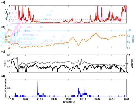
Figure 2. Temporal evolution of (a) the observed Vis (Vis_ob, in km) from BGMS, (b) Ta (in °C) and RH (in %), (c) wind direction (in °) and wind speed (in m s⁻¹), and (d) precipitation (in mm) from 1700 UTC 27 June to 0920 UTC 28 June 2022.

Vis changes revealed a pattern where Vis initially decreased at coastal stations and then at inland stations. This indicated that fog first reached the nearshore waters before advancing onto land in the early morning. Satellite imagery from the Himawari-8 satellite showed significant cloud coverage above the fog layer (Figure 3a,b) and precipitation was recorded at all stations during the event (Figure 3c). BGMS measured a cumulative rainfall of 22.9 mm, primarily occurring during two time periods: from 2000 to 2100 UTC on 27 June, and from 0300 to 0400 UTC on 28 June (Figure 2d).

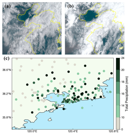
Figure 3. (a,b) display visible satellite imagery from the Himawari-8 satellite (Source: https://www.eorc.jaxa.jp/ptree/index.html (accessed on 11 December 2024)). (a) 0000 UTC on 28 June and (b) 0300 UTC on 28 June. (c) Scatter plot of cumulative precipitation (in mm) from automatic weather stations near BGMS throughout the fog process.

3.2. Fog Droplets Microphysical Characteristics

Based on the temporal changes in microphysical characteristics (Figure 4), we divided the sea fog process into four stages: Formation, development, maturity, and dissipation. The corresponding time and microphysical parameters for each stage are outlined in Table 1.

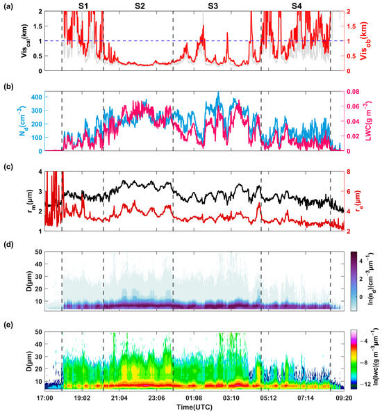
Figure 4. Temporal evolution of Vis and microphysical character. (a) The observed Vis (red line) and calculated Vis based on 1 min average fog DSD data (grey line), (b) the 1 min average N_d (blue line) and LWC (red line), (c) the 1 min average r_m (black line) and r_e (red line), (d) the 1 min average N_d spectrum, and (e) the 1 min average LWC spectrum. The labels S1 to S4 at the top of the figure indicate the four stages of the fog process: formation, development, maturity, and dissipation.

Table 1. Average, maximum, and minimum values of key characteristic parameters of the whole fog process and four stages.

Fog Stage	Time (UTC)	Vis (m)	Nd (cm−3)	LWC (g m−3)	rm (μm)	re (μm)
Whole Process	27 June 17:56−28 June 08:35	883 (147−15517)	190.62 (1.43−440.88)	0.026 (0.001−0.068)	2.84 (2.07−3.54)	3.44 (2.35−9.52)
Formation Stage (S1)	27 June 17:56−20:11	1961 (393−15517)	99.76 (1.43−259.10)	0.012 (0−0.030)	2.73 (2.46−3.04)	3.80 (2.91−9.52)
Development Stage (S2)	27 June 20:12−28 June 00:35	277 (170−929)	238.77 (75.76−381.19)	0.044 (0.007−0.067)	3.21 (2.48−3.54)	3.89 (2.93−5.07)
Maturity Stage (S3)	28 June 00:36−04:47	469 (147−2293)	248.58 (39.71−440.88)	0.031 (0.003−0.068)	2.81 (2.30−3.37)	3.33 (2.64−4.85)
Dissipation Stage (S4)	28 June 04:48−08:35	1368 (362−5758)	123.47 (10.40−256.77)	0.012 (0−0.037)	2.58 (2.07−3.01)	2.92 (2.35−4.10)

Note: The first row represents the mean values, with the parameter range indicated in parentheses (minimum−maximum).

The primary microphysical characteristics observed during the fog process were also presented in Table 1. The mean N_d was 190.62 cm⁻³, the mean LWC was 0.026 g m⁻³, the mean r_e was 3.44 μm, and the mean r_m was 2.84 μm. Compared to the sea fog process observed by Wang et al. [12], N_d in this event was higher, while LWC and r_m were lower, likely due to the presence of precipitation.

The microphysical structure changed significantly throughout the process, with Vis and microphysical parameters displaying roughly opposite trends. During the formation stage, Vis decreased notably, while N_d and LWC increased from 0, exhibiting low growth rates (Figure 4b). During the development stage, Vis remained below 1 km; the overall microphysical parameters were elevated, particularly droplet size, with r_m and r_e reaching significant values (Figure 4c). In the mature stage, microphysical characteristics fluctuated greatly, with both N_d and LWC reaching their maximum values throughout the entire process (Table 1). This increase was likely related to rising temperatures after sunrise over the coastal land. During the dissipation stage, Vis increased while all characteristic parameters decreased.

The 1 min average N_d spectrum indicated that fog droplets were primarily concentrated in sizes less than 10 μm (Figure 4d), while 1 min average LWC spectrum better represented the distribution of droplets with diameters ranging from 10 to 30 μm (Figure 4e). Over time, the droplet spectrum showed distinct changes. It broadened during the formation stage and exhibited pronounced bimodal characteristics in the development stage. In the mature stage, the intensity of the second peak reduced. Finally, the spectrum narrowed during the dissipation stage.

Table 2 presents a comparison of mean values and variability ranges for microphysical parameters in sea fog events observed at BGMS, Qingdao, and other coastal regions in China to better understand sea fog characteristics in our study area. The results reveal notable differences in microphysical characteristics across regions. Overall, Qingdao exhibited a relatively high mean N_d, second only to observations from the coastal area of Guangdong. However, the maximum N_d in both regions were similar, reaching approximately 400 cm⁻³. The mean LWC at BGMS was relatively low, significantly lower than in other regions except Guangxi. In terms of droplet size, Beilun had the largest mean r_m, followed by Qingdao.

Table 2. Comparison of sea fog microphysical characteristics between BGMS (Qingdao) and other coastal regions in China.

Observation Site and Time	Observation Instrument	Nd (cm−3)	LWC (g m−3)	rm (μm)
Qingdao, Shandong 27−28 June 2022	FM-120	190.62 (1.43−440.88)	0.026 (0.001−0.068)	2.84 (2.07−3.54)
Beilun, Zhejiang [25] 14−15 June 2021	FM-120	41.5 (0.31−212.93)	0.065 (0−0.64)	5.3 (1.75−11)
Xiamen, Fujian [26] 7 April 2019	FM-120	100 (0−468)	0.17 (0−1.35)	/
Maoming, Guangdong [27] 16−17 March 2008	FM-100	326.6 (15−422.6)	0.058 (0.010−0.64)	1.5 (1.2−2.45)
Zhanjiang, Guangdong [28] 23−24 February 2011	FM-100	248.0 (3−354)	0.102 (0.001−0.257)	2.6 (1.55−3.9)
Weizhou Island, Guangxi [29] 28 February 2021	FM-100	76.7 (10.6−454.9)	0.006 (0.001−0.03)	2.0 (1.9−2.2)

Note: “/” indicates the values are not shown in the reference.

Table 2. Comparison of sea fog microphysical characteristics between BGMS (Qingdao) and other coastal regions in China.

Observation Site and Time	Observation Instrument	Nd (cm−3)	LWC (g m−3)	rm (μm)
Qingdao, Shandong 27−28 June 2022	FM-120	190.62 (1.43−440.88)	0.026 (0.001−0.068)	2.84 (2.07−3.54)
Beilun, Zhejiang [25] 14−15 June 2021	FM-120	41.5 (0.31−212.93)	0.065 (0−0.64)	5.3 (1.75−11)
Xiamen, Fujian [26] 7 April 2019	FM-120	100 (0−468)	0.17 (0−1.35)	/
Maoming, Guangdong [27] 16−17 March 2008	FM-100	326.6 (15−422.6)	0.058 (0.010−0.64)	1.5 (1.2−2.45)
Zhanjiang, Guangdong [28] 23−24 February 2011	FM-100	248.0 (3−354)	0.102 (0.001−0.257)	2.6 (1.55−3.9)
Weizhou Island, Guangxi [29] 28 February 2021	FM-100	76.7 (10.6−454.9)	0.006 (0.001−0.03)	2.0 (1.9−2.2)

Note: “/” indicates the values are not shown in the reference.

3.3. Comparison of the Effect of Large and Small Droplets

Based on the average r_e in this case, we defined an empirical threshold of 3.5 μm to classify fog droplets as “small” or “large”. The N_d of small (blue) and large (red) droplets were calculated at 1 min intervals and plotted against the total N_d (Figure 5a). The regression lines were y = 0.81x + 11.22 (R² = 0.95) for small droplets and y = 0.19x − 11.22 (R² = 0.53) for large droplets, indicating that approximately 81% of the droplets were small.

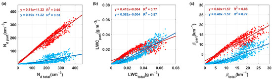
Figure 5. (a) The 1 min average N_d of small droplets (red dots) and large droplets (blue dots) as a function of total N_d, (b) the 1 min average LWC of small droplets (red dots) and large droplets (blue dots) as a function of total LWC, and (c) the 1 min average β_ext of small droplets (red dots) and large droplets (blue dots) as a function of total β_ext.

Similarly, the 1 min average LWC (Figure 5b) and β_ext (Figure 5c) were calculated for both size categories. The results showed that large droplets accounted for 58% of the total LWC, while small droplets contributed 60% of the total β_ext. This indicated that small droplets dominated N_d and played a critical role in visibility attenuation, whereas large droplets had a more significant influence on LWC.

3.4. Analytical Expression for Fog DSD

Figure 6 shows fog DSD characteristics at each stage of the fog process, specifically where the observed visibility was below 1 km. Consistent with the changes shown in Figure 4, the average spectrum first rose and then declined over time. During the development stage, there was a marked increase in the number of droplets across all sizes, leading to the widest droplet spectrum.

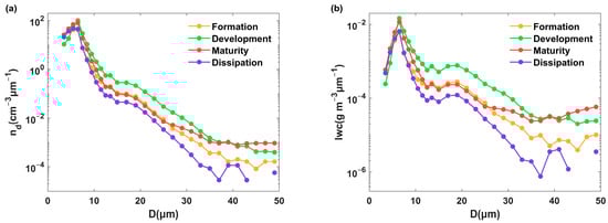
Figure 6. The mean fog DSD at different stages of the fog process. (a) N_d spectrum distribution and (b) LWC spectrum distribution. The average spectrum is calculated using data with Vis below 1 km.

The average DSD of the whole fog process can be fitted using the Gamma function:

$$\mathrm{n}\left(\mathrm{r}\right)=9.12·{\mathrm{r}}^{26.68}·{\mathrm{e}}^{-9.07\mathrm{r}},$$

(11)

where r and n(r) represent the radius and the corresponding N_d at that radius, respectively.

To describe the fog DSD more accurately, Wang et al. [12] proposed a new function, the G-exponential function:

$$\mathrm{n}(\mathrm{r})={\mathrm{a}}_1{\mathrm{e}}^{-{({\displaystyle \frac{\mathrm{r}-{\mathrm{b}}_1}{{\mathrm{c}}_1}})}^2}+{\mathrm{a}}_2{\mathrm{e}}^{-{({\displaystyle \frac{\mathrm{r}-{\mathrm{b}}_2}{{\mathrm{c}}_2}})}^2},$$

(12)

where a₁, b₁, c₁, a₂, b₂, and c₂ are the parameters, and r and n(r) are defined as stated in the previous equation.

The average spectrum can be described as:

$$\mathrm{n}(\mathrm{r})=142.34{\mathrm{e}}^{-{({\displaystyle \frac{\mathrm{r}-3.04}{0.19}})}^2}+45.96{\mathrm{e}}^{-{({\displaystyle \frac{\mathrm{r}-2.80}{1.06}})}^2},$$

(13)

A comparison of the G-exponential function and the Gamma function reveals their effects during different stages of the fog event (Table 3). The G-exponential function is more suitable for the droplet spectrum distribution in this case, corroborating the results of Wang et al. [13]. The fitting performance exhibits significant variability across different stages, but it remains robust during periods with Vis below 1 km, with R² values exceeding 90%.

Table 3. Fit quality comparison between two DSD functions.

Function Type	Accuracy Metrics	Whole Process	Formation Stage	Development Stage	Maturity Stage	Dissipation Stage
Gamma	RMSE (km)	5.34	8.91	7.66	6.28	8.12
	R2	0.926	0.49	0.87	0.91	0.62
G-exponential	RMSE (km)	0.94	8.22	5.42	3.34	7.45
	R2	0.998	0.57	0.93	0.97	0.68

3.5. Comparison of the Calculated Vis with Different Methods

When a LWC is specified in a fog model, n(r) can be computed using Equations (11) and (13). This enables the calculation of Vis based on Equation (5), with the results denoted as Vis_Gam and Vis_Gex. Additionally, visibility parameterization schemes can be established based on the power–law relationships of microphysical characteristics (Table 4). An evaluation of visibility prediction results from different methods shows that the visibility parameterization scheme using both N_d and LWC results in a smaller MRE than those using either N_d or LWC alone.

Table 4. The fitting effect of different parameterization schemes.

Name	Function	MAE (km)	RMSE (km)
VisGam	/	0.16	0.24
VisGex	/	0.15	0.23
VisGN	44.989(Nd) −1.1592 [30]	0.33	0.39
VisEdg	0.024(LWC) −0.65 [31]	0.17	0.23
Visk84	0.027(LWC) −0.88 [32]	0.26	0.36
VisGNL	1.002(Nd·LWC) −0.6743 [30]	0.13	0.27
VisFRAM	0.8771(Nd·LWC) −0.49034 [4]	0.10	0.18

Figure 7 presents the temporal evolutions of Vis_Gex, Vis_GN, Vis_k84, Vis_FRAM, and the observed Vis, indicating that Vis_FRAM has the lowest MAE and RMSE, in turn demonstrating the best Vis prediction performance, followed by Vis_Gex.

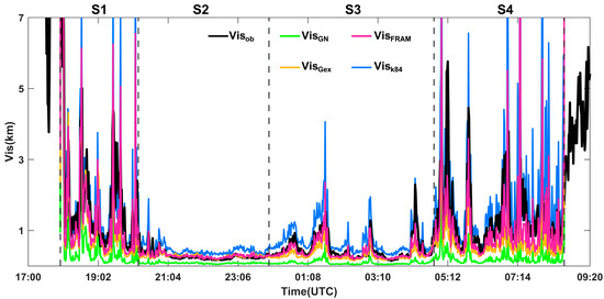
Figure 7. Temporal evolution of visibility (solid line, in m) from BGMS during the sea fog event from 1756 UTC 27 June to 0835 UTC 28 June 2022. Vis_ob is the observed Vis. Vis_Gex is obtained from Equation (13); Vis_GN, Vis_k84, and Vis_FRAM are obtained from Table 3. The labels S1 to S4 at the top of the figure indicate the four stages of the fog process: formation, development, maturity, and dissipation.

4. Discussion

The most notable characteristic of this sea fog event is the accompanying precipitation. This precipitation maintained RH at 100% throughout the process and coincided with rising temperatures (Figure 2). The precipitation provided ample moisture to the lower layer, maintaining a high water vapor content and supporting the extended duration of the fog. In contrast, observations by Wang et al. [12] during a spring sea fog event also showed high RH, yet indicated a significant temperature drop of nearly 2 °C, which differs from the rising temperatures observed in our case.

During this sea fog event, the main periods of precipitation occurred from 2000 to 2100 UTC on 27 June and from 0300 to 0400 UTC on 28 June (Figure 2d). The changes in LWC spectrum distribution (Figure 4e) clearly show that after 21:00 UTC on 27 June, there was a significant increase in large droplet formation, resulting in a relatively strong bimodal structure. A similar phenomenon was observed after 0420 UTC on 28 June; however, due to the rise in temperature after sunrise, the fog process entered a dissipation stage, leading to a reduction in the width of the droplet spectrum and a less pronounced bimodal distribution compared to the first stage. Additionally, compared to the microphysical characteristics observed by Wang et al. [12], N_d was higher, while LWC and r_m were lower. These differences in microphysical characteristics may also be influenced by the precipitation present during this summer sea fog event, but a deeper understanding requires additional observational data.

5. Conclusions

The microphysical characteristics of a summer sea fog event with precipitation along the west coast of the Yellow Sea were observed at BGMS from 27 June to 28 June 2022. Combined with meteorological data, the microphysics of this event were analyzed, yielding the following conclusions:

• The fog event lasted 880 min, beginning at 1756 UTC on 27 June and dissipating by 0835 UTC on June 28 (LST = UTC + 8 h). Significant precipitation occurred during two periods: 2100–2200 UTC on June 27 and 0300–0400 UTC on 28 June. Although the precipitation caused fluctuations in visibility, it did not disrupt the formation or persistence of the fog.
• The observed microphysical parameters included an average N_d of 190.62 cm⁻³, LWC of 0.026 g m⁻³, r_m of 2.84 μm, and r_e of 3.44 μm. Using the average r_e as a threshold, droplets were classified as “small” or “large”. Small droplets dominated N_d (81%) and contributed significantly to visibility attenuation (60% of β_ext), while large droplets, though fewer in number, accounted for 58% of LWC.
• The fog DSD throughout the fog event was better represented by a G-exponential distribution than by a Gamma distribution. The fog process was divided into four stages: formation, development, maturity, and dissipation. During formation, droplet sizes increased. The development stage exhibited a pronounced bimodal spectrum, with the second peak weakening in maturity. By dissipation, droplet quantities decreased, narrowing the spectrum.
• A comparison of visibility parameterization methods reveals that incorporating both N_d and LWC yields a smaller MRE compared to using either parameter alone. Among the evaluated methods, Vis_FRAM demonstrates the lowest MAE and RMSE, indicating superior visibility prediction performance, followed by Vis_Gex.

This study investigates the microphysical characteristics of a precipitation-associated sea fog event along the west coast of the Yellow Sea and provides detailed parameterization for Vis estimation. While the findings are based on a single on-site fog event, potential variability may exist. Additionally, factors such as aerosol influence on N_d and LWC were not addressed. The specific impact of precipitation on sea fog microphysics requires further investigation. To address these limitations, long-term field observations at BGMS and more comprehensive instrumentation will be employed in future studies.

References

- Wang, B.H. Sea Fog; China Ocean Press: Beijing, China, 1985; p. 330. [Google Scholar]
- Koračin, D.; Dorman, C.E.; Lewis, J.M.; Hudson, J.G.; Wilcox, E.M.; Torregrosa, A. Marine fog: A review. Atmos. Res. 2014, 143, 142–175. [Google Scholar] [CrossRef]
- Gultepe, I.; Tardif, R.; Michaelides, S.; Cermak, J.; Bott, A.; Bendix, J.; Müller, M.D.; Pagowski, M.; Hansen, B.; Ellrod, G.P.; et al. Fog research: A review of past achievements and future perspectives. Pure Appl. Geophys. 2007, 164, 1121–1159. [Google Scholar] [CrossRef]
- Gultepe, I.; Pearson, G.; Milbrandt, J.A.; Hansen, B.; Platnick, S.; Taylor, P.; Gordon, M.; Oakley, J.P.; Cober, S.G. The fog remote sensing and modeling (FRAM) field project. Bull. Am. Meteorol. Soc. 2009, 90, 341–360. [Google Scholar] [CrossRef]
- Jung, S.; Qin, X.; Oh, C. A risk-based systematic method for identifying fog-related crash prone locations. Appl. Spat. Anal. 2019, 12, 729–751. [Google Scholar] [CrossRef]
- Eldridge, R.G. A few fog drop-size distributions. J. Atmos. Sci. 1961, 18, 671–676. [Google Scholar] [CrossRef]
- Gultepe, I.; Milbrandt, J.A. Probabilistic parameterizations of visibility using observations of rain precipitation rate, relative humidity, and visibility. J. Appl. Meteorol. Climatol. 2010, 49, 36–46. [Google Scholar] [CrossRef]
- Gultepe, I.; Heymsfield, A.J.; Fernando, H.J.S.; Pardyjak, E.; Dorman, C.E.; Wang, Q.; Creegan, E.; Hoch, S.W.; Flagg, D.D.; Yamaguchi, R.; et al. A review of coastal fog microphysics during C-FOG. Bound.-Layer Meteorol. 2021, 181, 227–265. [Google Scholar] [CrossRef]
- Gultepe, I.; Kuhn, T.; Pavolonis, M.; Calvert, C.; Gurka, J.; Heymsfield, A.J.; Liu, P.S.K.; Zhou, B.B.; Ware, R.; Ferrier, B.; et al. Ice fog in Arctic during FRAM-ice fog project: Aviation and nowcasting applications. Bull. Am. Meteorol. Soc. 2014, 95, 211–226. [Google Scholar] [CrossRef]
- Fernando, H.J.S.; Gultepe, I.; Dorman, C.; Pardyjak, E.; Wang, Q.; Hoch, S.; Richter, D.; Creegan, E.; Gaberšek, S.; Bullock, T.; et al. C-FOG: Life of coastal fog. Bull. Am. Meteorol. Soc. 2021, 176, 1977–2017. [Google Scholar] [CrossRef]
- Zhang, S.P.; Bao, X.W. The main advances in sea fog research in China. Period. Ocean Univ. China 2008, 38, 359–366. (In Chinese) [Google Scholar] [CrossRef]
- Wang, S.K.; Yi, L.; Zhang, S.P.; Shi, X.M.; Chen, X.Y. The microphysical properties of a sea-fog event along the west coast of the Yellow Sea in spring. Atmosphere 2020, 11, 413. [Google Scholar] [CrossRef]
- Spiegel, J.K.; Zieger, P.; Bukowiecki, N.; Hammer, E.; Weingartner, E.; Eugster, W. Evaluating the capabilities and uncertainties of droplet measurements for the fog droplet spectrometer (FM-100). Atmos. Meas. Technol. 2012, 5, 2237–2260. [Google Scholar] [CrossRef]
- Liu, Y.L.; Zhao, J.P. A Correction Algorithm for Atmospheric Visibility Based on Fog Droplet Size Data Obtained on a Moving Ship During 2016 Arctic Cruise. J. Ocean Univ. China 2019, 18, 596–604. [Google Scholar] [CrossRef]
- Koike, M.; Ukita, J.; Strom, J.; Tunved, P.; Shiobara, M.; Vitale, V.; Lupi, A.; Baumgardner, D.; Ritter, C.; Hermansen, O.; et al. Yearround in situ measurements of arctic low-level clouds: Microphysical properties and their relationships with aerosols. Geophys. Res. Atmos. 2019, 124, 1798–1822. [Google Scholar] [CrossRef]
- Duplessis, P.; Bhatia, S.; Hartery, S.; Wheeler, M.J.; Chang, R.Y.-W. Microphysics of aerosol, fog and droplet residuals on the Canadian Atlantic coast. Atmos. Res. 2021, 264, 105859. [Google Scholar] [CrossRef]
- Hansen, J.E.; Travis, L.D. Light scattering in planetary atmospheres. Space Sci. Rev. 1974, 16, 527–610. [Google Scholar] [CrossRef]
- Reid, J.S.; Hobbs, P.V.; Rangno, A.L.; Hegg, D.A. Relationships between cloud droplet effective radius, liquid water content, and droplet concentration for warm clouds in Brazil embedded in biomass smoke. J. Geophys. Res. 1999, 104, 6145–6153. [Google Scholar] [CrossRef]
- Koschmieder, H. Theorie der horizontalen Sichtweite. In Beiträge zur Physik der freien Atmosphäre; Keim & Nemnich: Diedorf, Germany, 1924; Volume 12, pp. 33–53. [Google Scholar]
- McCartney, E.J. Optics of the Atmosphere: Scattering by Molecules and Particles; John Wiley and Sons, Inc.: New York, NY, USA, 1976. [Google Scholar] [CrossRef]
- Stoelinga, M.T.; Warner, T.T. Nonhydrostatic, mesobeta-scale model simulations of cloud ceiling and visibility for an east coast winter precipitation event. J. Appl. Meteorol. Climatol. 1999, 38, 385–404. [Google Scholar] [CrossRef]
- Mie, G. Beiträge zur Optik trüber Medien, speziell kolloidaler Metallösungen. Ann. Phys. 1908, 330, 377–445. [Google Scholar] [CrossRef]
- Draper, N.R.; Smith, H. Applied Regression Analysis, 2nd ed.; John Wiley and Sons: New York, NY, USA, 1981. [Google Scholar] [CrossRef]
- Goodin, D.S. The Cambridge Dictionary of Statistics; Cambridge University Press: Cambridge, UK, 2006. [Google Scholar]
- He, J.X.; Ren, X.Y.; Wang, H.; Shi, Z.; Zhang, F.G.; Hu, L.J.; Zeng, Q.Y.; Jin, X. Analysis of the Microphysical Structure and Evolution Characteristics of a Typical Sea Fog Weather Event in the Eastern Sea of China. Remote Sens. 2022, 14, 5604. [Google Scholar] [CrossRef]
- Zhang, W.; Chen, D.H.; Hu, Y.J.; Xun, A.P.; Jiang, Y.C.; Sun, X.J. Microphysical Structure Analysis of a Spring Sea Fog Event in Southern Coastal Area of Fujian. Meteorol. Mon. 2021, 47, 157–169. (In Chinese) [Google Scholar]
- Huang, H.J.; Huang, J.; Mao, W.K.; Liao, F.; Li, X.N.; Lü, W.H.; Yang, Y.Q. Evolution characteristics of water content in sea fog and its relationship with atmospheric horizontal visibility in Maoming area. Haiyang Xuebao 2010, 32, 40–53. (In Chinese) [Google Scholar]
- Lv, J.J.; Niu, S.J.; Zhang, Y.; Xu, F. Evolution characteristics of the macro-/micro-structure and the boundary layer during a spring heavy sea fog episode in Donghai Island in Zhanjiang. Acta Meteor. Sin. 2014, 2, 350–365. (In Chinese) [Google Scholar]
- Lu, Q.Q.; Zheng, F.Q.; Bi, R.D.; Lu, X.T. Analysis of four outfield observation data of sea fog on Weizhou Island in 2021. J. Meteor. Res. Appl. 2013, 27, 609–622. (In Chinese) [Google Scholar]
- Gultepe, I.; Müller, M.D.; Boybeyi, Z. A new visibility parameterization for warm-fog applications in numerical weather prediction models. J. Appl. Meteorol. Climatol. 2006, 45, 1469–1480. [Google Scholar] [CrossRef]
- Eldridge, R.G. Haze and fog aerosol distributions. J. Atmos. Sci. 1966, 23, 605–613. [Google Scholar] [CrossRef]
- Kunkel, B.A. Parameterization of droplet terminal velocity and extinction coefficient in fog models. J. Appl. Meteorol. Climatol. 1984, 23, 34–41. [Google Scholar] [CrossRef]
Disclaimer/Publisher’s Note: The statements, opinions and data contained in all publications are solely those of the individual author(s) and contributor(s) and not of MDPI and/or the editor(s). MDPI and/or the editor(s) disclaim responsibility for any injury to people or property resulting from any ideas, methods, instructions or products referred to in the content. |
© 2025 by the authors. Licensee MDPI, Basel, Switzerland. This article is an open access article distributed under the terms and conditions of the Creative Commons Attribution (CC BY) license (https://creativecommons.org/licenses/by/4.0/).