Article

Comparing Reflectivity from Space-Based and Ground-Based Radars During Detection of Rainbands in Two Tropical Cyclones

by
Corene J. Matyas
1,*,
Stephanie E. Zick
2 and
Kimberly M. Wood
3
1
Department of Geography, University of Florida, Gainesville, FL 32611, USA
2
Department of Geography, Virginia Tech, Blacksburg, VA 24061, USA
3
Department of Hydrology and Atmospheric Sciences, University of Arizona, Tucson, AZ 85721, USA
*
Author to whom correspondence should be addressed.
Atmosphere 2025, 16(3), 307; https://doi.org/10.3390/atmos16030307
Submission received: 27 December 2024 / Revised: 6 February 2025 / Accepted: 26 February 2025 / Published: 6 March 2025

Abstract

:
With varying tangential winds and combinations of stratiform and convective clouds, tropical cyclones (TCs) can be difficult to accurately portray when mosaicking data from ground-based radars. This study utilizes the Dual-frequency Precipitation Radar (DPR) from the Global Precipitation Measurement Mission (GPM) satellite to evaluate reflectivity obtained using four sampling methods of Weather Surveillance Radar 1988-Doppler data, including ground radars (GRs) in the GPM ground validation network and three mosaics, specifically the Multi-Radar/Multi-Sensor System plus two we created by retaining the maximum value in each grid cell (MAX) and using a distance-weighted function (DW). We analyzed Hurricane Laura (2020), with a strong gradient in tangential winds, and Tropical Storm Isaias (2020), where more stratiform precipitation was present. Differences between DPR and GR reflectivity were larger compared to previous studies that did not focus on TCs. Retaining the maximum value produced higher values than other sampling methods, and these values were closest to DPR. However, some MAX values were too high when DPR time offsets were greater than 120 s. The MAX method produces a more consistent match to DPR than the other mosaics when reflectivity is <35 dBZ. However, even MAX values are 3–4 dBZ lower than DPR in higher-reflectivity regions where gradients are stronger and features change quickly. The DW and MRMS mosaics produced values that were similar to one another but lower than DPR and MAX values.

1. Introduction

Across the United States, a network of ground-based radars comprised of Weather Surveillance Radar-1988 Doppler (WSR-88D, WSR hereafter) units continuously scans the atmosphere to monitor weather systems [1]. These radars provide data at high spatial and temporal resolution, completing volumetric scans comprised of 360° radial sweeps at tilts of 0.5–20° every 4–6 min when precipitation is present. The collection of sweeps is referred to as a volume coverage pattern (VCP). Within a sweep, observations are available every 250 m radially and 0.5–1° in azimuth. However, this conical scanning geometry poses challenges in detecting changes within convective weather systems such as tropical cyclones (TCs) as data densities vary greatly with distance to radar. This is particularly true for convective clouds: their narrow horizontal and tall vertical structures yield sharp gradients in reflectivity. For example, with a scan elevation of 0.5°, which is closest to the ground, at 30 km from the radar, the beam width is 0.5 km, and the beam height above the antenna ranges from 0.1 km at the bottom to 0.6 km at the top. At this distance, multiple beams along the same elevation scan sample the cloud horizontally to reveal gradients in reflectivity, and multiple elevation scans can provide details on changing rain rates with height. However, using the same scan elevation at a 200 km distance, the beam is 3.2 km wide and its height ranges from 2.7 (bottom) to 5.9 (top) km; thus, heavy rain at the bottom of the cloud cannot be detected. Additionally, because a single reflectivity value represents this larger vertical and horizontal cloud section, sharp gradients within that volume cannot be detected. Such limitations highlight the importance of considering the distance between the radar and the TC rainfall regions in detecting the structure of its clouds.
Additional limitations present observational challenges for individual radars. The geometry of radar beams poses problems with accurate detection of weather systems due to beam refraction, lack of beam filling, beam blockage, and limits on beam height coupled with the inability to tilt directly upwards [2]. Although these S-band (10 cm wavelength) radars suffer less from attenuation than X- or C-band weather radars [3], it can still be an issue, especially after the beam through a large region of high rain rates [4]. Research has shown that when the radome lacks hydrophobicity, water filming can impact antenna performance [5,6]. Additionally, calibration drifts can result in transmissions of power that are higher or lower over time [7,8], thus running “hot or “cold” [9,10]. Month-to-month drifts exceeding 1 dB occasionally occurred over a four-year study of five WSRs [11].
To reduce the effects of these factors, it is advantageous to examine data from neighboring radars when scanning a TC. Also, combining data from multiple WSR units is necessary to observe meso- to synoptic-scale weather systems as they develop and move. For example, mosaics that encompass an entire TC facilitate object-based methods to track rainfall regions in the TC’s inner core and outer rainbands as they rapidly evolve during landfall [12,13]. One way to accomplish this is to grid values to create a mosaic [14,15]. The higher spatial resolution near the radar means that centers of data bins are close enough to permit multiple observations to fall within one 1 km3 grid box, which necessitates decisions on what the final value should be. Two approaches are generally used to determine the final value: researchers have utilized the highest value [12,16] and calculated various weighted averages [14,17,18]. The lower density of data farther from the radar necessitates interpolation to fill empty grid boxes using methods such as nearest neighbor [17,18]. Temporal offsets in scans and varied VCPs among neighboring radars can also pose problems as those scan patterns and timings are independent of one another. In addition, forecasters may employ Supplemental Adaptive Intra-Volume Scanning (SAILS) [19], where the lowest scan elevation is revisited one or more times during a VCP to provide more data in the lowest levels, but it delays completion of the VCP [20], and these decisions are made independent of scan patterns undertaken by neighboring radars.
Any weather system moving and/or quickly changing poses a challenge for the mosaicking process due to temporal offsets in neighboring WSR scans. TCs pose unique challenges not only due to their varying forward speeds (ranging from 1 to 29 ms−1 at landfall in the Atlantic basin) but also because their cyclonic rotational motion has varying velocities over their rain fields, which can span >800 km when making landfall over the U.S [21]. For example, when Hurricane Dorian (2019) made landfall over the Bahamas with maximum sustained winds >82 ms−1 located 10 km from the center, tropical-storm-force winds (17 ms−1) extended 200 km outward on its eastern side, creating a large change in rotational velocity that would be difficult to accurately portray if neighboring radars detected the same convective cell at different times. In the eyewall, the angular motion translates to moving one kilometer in 0.205 min, while at the radius of tropical-storm-force winds, it takes 0.98 min to move one kilometer. Willoughby et al. [22] estimated that a parcel of air takes four hours to traverse the TC eyewall at 60 km from the storm center, which equates to 1.5 km per minute. This fast motion could cause a convective cell to be detected by beams at different azimuths for some tilts as a VCP scan can take 4–6 min. Also, as neighboring radars are not in sync, temporal offsets greater than one minute are common when neighboring WSRs scan the same location. In addition, given the sharp horizontal reflectivity gradient in convective regions, temporal offsets can be a larger problem compared with stratiform precipitation where horizontal changes are more gradual. All of these conditions point to the need for in-depth studies of mosaicking strategies for observing TCs.
To help identify calibration bias in ground-based radars, scientists have used precipitation radars aboard the Tropical Rainfall Measuring Mission (TRMM) and Global Precipitation Measurement Mission (GPM) satellites as independent observations (e.g., [23,24,25]), although their spatial and temporal characteristics differ from the WSR. The more modern Dual-frequency Precipitation Radar (DPR) aboard GPM has two radars: Ku− (13.6 GHz) and Ka-bands (35.5 GHz). Observations cover a footprint of ~5 km over a 245-km wide swath with a vertical resolution of 250 m. Although the GPM satellite passes overhead quickly enough for a synoptic-scale system to be observed instantaneously [26], the limited swath width and revisit time of 1–2 days means that only a portion of the system will be sampled during each overpass; thus, short-term changes in fine-scale features cannot be detected. The DPR suffers less from beam widening as the extent of measurements in the vertical direction occurs 0–20 km from the Earth’s surface [26] compared to the 200+ km horizontal extent for WSRs. Updates to DPR calibration relative to WSR observations have been stable over time, varying by less than 1 dB over four years of analysis [27]. Studies have shown that DPR and WSR observations are highly correlated (~0.9 for the Ku band). Calculations of DPR-WSR yielded biases of −1.1 to 2.5 dB over four years for five near-coast radars [11] and biases of 1.68–2.2 dB for three years of data in stratiform precipitation over the northern U.S. for three WSR units [28]. For six years of observations over 136 WSR sites, DPR values were 2.4 dB higher than WSR observations [24]. However, these previous studies do not specifically examine observations from TCs, although TCs are most likely present in the analysis conducted by [11].
Given the challenges for the WSR network to observe TCs and the dearth of studies examining TCs using DPR and WSR data, this study utilizes DPR observations as the baseline against which we examine reflectivity values from WSR stations. The WSR values are derived from four sampling methods during two landfalling TCs with different storm-relative and environmental conditions. These four WSR sampling methods come from three sources (Table 1). For the first source, we examine reflectivity from ground radars (GRs) in the GPM Ground Validation System (GVS) Validation Network (VN) as these values are from DPR and WSR beams matched in location and time. We then compare DPR values with three mosaicked WSR datasets where the timestamp of the mosaics occurs as close as possible to the DPR overpass time. The second source, the Multi-Radar/Multi-Sensor (MRMS) dataset, is a publicly available radar data mosaic with high spatial and temporal resolution. Finally, we use data from the third source, WSR Level II data, to create two additional mosaics at the same spatial resolution as MRMS by (a) retaining the maximum reflectivity value (MAX) for a given grid cell regardless of which radar it comes from, and (b) performing the analysis again but employing a distance-weighting algorithm (DW) prior to averaging reflectivity values inside each cell. The novelty of this research lies in the focus on TCs, using DPR to compare mosaics of WSR data in addition to the GPM GVS VN, and creating two different mosaics to compare the methods of retaining the maximum value and using a weighted average.
We hypothesize that values in the GR dataset will be closer to DPR than the DW and MRMS, given the averaging and interpolation that occur during the mosaicking process [10] and that retaining higher values from neighboring radars in the MAX mosaics could lead to less error when neighboring radars scan the region at a time closer to the overpass and/or when the wet radome effect occurs. We also hypothesize that differences will occur at each radar due to its pattern and timing of scans, whether it is raining at the radar, and which part of the TC is being sampled by the radar. We test these hypotheses by calculating reflectivity differences between DPR and the four WSR sampling methods and by performing a test for repeated measures that determines which of the five datasets are statistically significantly similar. All tests are performed separately for each WSR. We also explore the impact of time offsets in the creation of the MRMS mosaic in the context of a major hurricane in which raining regions move more quickly around the circulation center compared to a weakening tropical storm in which tangential motion is slower.

2. Materials and Methods

2.1. Materials

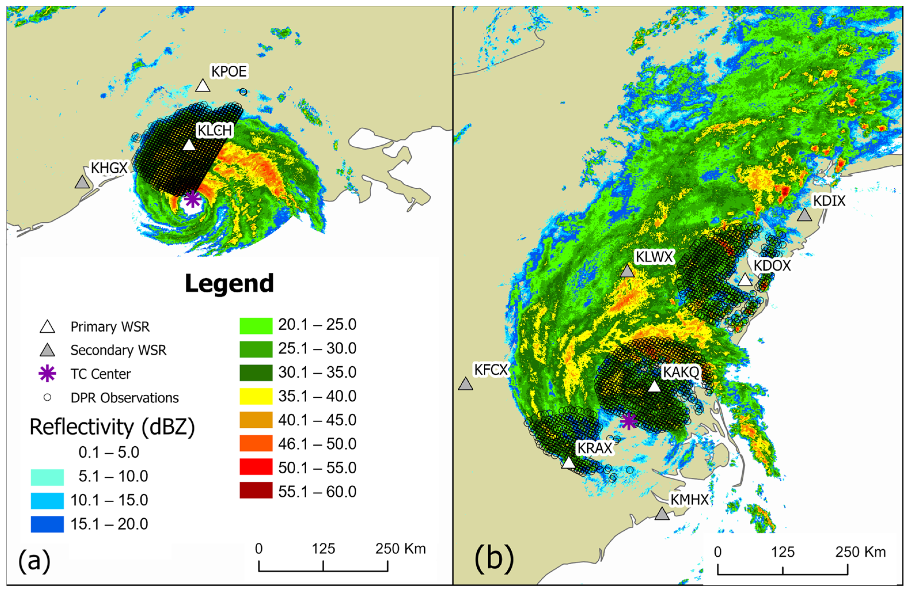
2.1.1. TC-Specific Information

We examine data from two contrasting TCs that made landfall over the U.S. in August 2020. We selected Laura (Figure 1a) and Isaias (Figure 1b) for analysis as each was in a different stage of development and moving through different thermodynamic and dynamic conditions. TC position, intensity, extent of hurricane and gale-force winds, and forward velocity are obtained from the International Best Track Archive for Climate Stewardship (IBTrACS) version 4 [29].
Hurricane Laura made landfall over Louisiana on 27 August at 0600 UTC as a Category 4 storm [30]. The DPR overpass occurred at 0300 UTC, and though it did not observe the circulation center, it did collect data over the western eyewall (Figure 1a). Laura was at its lifetime maximum intensity (67 ms−1), which is in the top 2% for maximum sustained winds at landfall in the Atlantic basin. It was moving at 7.2 ms−1, and tropical storm-force winds extended 165 km, and hurricane-force winds extended 65 km from the center in its northwestern quadrant, the region best observed by the DPR overpass.
Isaias made landfall as a Category 1 hurricane over North Carolina at 0000 UTC on 4 August, weakening to tropical storm strength shortly thereafter [31]. The DPR passed over the TC center at 0852 UTC and sampled a long swath that included the TC’s outer rainbands interacting with a stationary front northeast of the TC center (Figure 1b). At the time, maximum sustained winds were 31 ms−1, and Isaias was beginning to transition into an extratropical cyclone. Thus, its forward speed was high at 15 m s−1, which is among the top 8% of forward velocities for landfalling TCs in the North Atlantic basin since 1851. Tropical storm-force winds extended to 200 km from the center in its northeast quadrant, the region best observed by the DPR overpass.

2.1.2. Data from the Ground Validation Network

The National Aeronautics and Space Administration (NASA) maintains the GPM GVS VN [25] that provides geometrically matched datasets between DPR standard Level 2 products (2ADPR) and Level II data from WSRs. From this database (https://gpm-gv.gsfc.nasa.gov/, accessed on 7 July 2021), we obtained (a) reflectivity from the DPR and (b) volume-matched reflectivity values for ground-based radars (GRs) (Table 1). Pertaining to (a), although the DPR consists of Ku− (13.6 GHz) and Ka-bands (35.5 GHz), we use the DPR normal scan matchups derived from the Ku-band radar reflectivity with attenuation correction due to these data having the widest spatial coverage. As previously stated, observations cover a footprint of ~5 km over a 245-km wide swath with a vertical resolution of 250 m. The minimum detectable reflectivity of DPR’s Ku-band is 12–13 dBZ [32]. In the database, DPR-GR matchups are only generated during “significant precipitation events” when at least 100 Ku-DPR rays are identified as “rain certain” within 100 km of a GR.
For (b), volume-matched reflectivities from the WSRs were also taken from the GPM GVS VN (Table 1). As previously mentioned, the WSRs have a range resolution of 0.25 km and azimuth resolution of 0.5–1°, and in the GPM GVS VN, quality control of these GR data is performed by NASA staff. Only intersections <100 km from a GR are included in the database to limit the effects of beam bending due to nonstandard atmospheric refraction. Reflectivity averages are calculated at the geometric intersection of DPR rays with individual GR sweeps [33]. DPR gates between the half-power GR beam points are linearly averaged vertically, while GR is averaged horizontally over the circular area of the DPR beam with a Gaussian inverse distance weight. As no other gridding, interpolation, or smoothing occurs, values are only produced where both instruments take observations. The database provides reflectivity values with latitude, longitude, and altitude, allowing the values to be plotted as points.
Given that the DPR travels at a speed of approximately 450 km per minute, it takes about 27 s to fly the 200-km diameter across which data are utilized from each GR. In contrast, the collection of sweeps that occurs as a WSR is tilted through different angles can take 4–6 min to complete when in precipitation mode. Thus, temporally, the GR volume scan closest to the time of the DPR overpass is utilized in the database. For our study, we obtained from this database reflectivity values from the DPR, two GRs that sampled Laura (KLCH and KPOE), and three GRs that sampled Isaias (KAKQ, KDOX, KRAX), which we refer to as primary radars in the study (Figure 1). The points where these values are available for each radar are denoted with circles in Figure 1. The database also labels each point as stratiform or convective [25] using the method described by Iguchi et al. [34]. We noted the timestamp for each GR to ensure that our mosaics encompass the same set of sweeps as the GPM GVS VN. Figure 2a,c show the reflectivity values from the DPR and GR for Laura, while Figure 3a,c show these values for Isaias.

2.1.3. Mosaic Datasets

Next, we utilize data from three WSR mosaicking methods to compare with these matched data points from GPM GVS VN. For the two mosaics that we created (Table 1), we imported Level II reflectivity data from radars located within 500 km of each TC center. We obtained these data from Amazon Web Service (AWS) S3 Explorer (https://s3.amazonaws.com/noaa-nexrad-level2/index.html, URL accessed 2 December 2023). We also incorporated data from the MRMS (Table 1). Details on the Map Reduce methodology used to create the MRMS mosaic are available from Lakshmanan and Humphrey [35]. Although several methods for handling multiple observations for a single location are described, neither the paper nor the MRMS website (https://vlab.noaa.gov/web/wdtd/-/wsr-88d-constant-altitude-reflectivity-mosaic?selectedFolder=668051, URL accessed 28 November 2023) identifies which strategy (e.g., nearest-neighbor mapping in range and azimuth, applying weights according to an exponential function that decreases with distance to the radar) is used to determine the value of each grid cell. From MRMS, mosaics of WSR values are available on a 0.01° latitude × 0.01° longitude grid at 31 vertical levels every two minutes. We utilized reflectivity values at 3 km above ground level, which is below the brightband according to data in the GPM GVS VN. When we compared datasets at multiple altitudes, including 2.5, 3, 3.5, and 4 km, the statistical assessment was highly similar across all altitudes. As a result, we present our findings at 3 km in this manuscript as they are representative of this layer of the troposphere. We utilize data from the timestamps 0302 UTC (Laura) and 0854 UTC (Isaias), as these time steps should capture the VCPs during each DPR overpass.

2.2. Methods

2.2.1. Mosaic Creation and Extraction of Points

This section describes the techniques we employed to create two mosaics of WSR reflectivity for each TC, the details of which can be found in [36,37]. Temporally, our code only utilizes VCPs that begin before the time we select. Thus, we use 0302 UTC for Laura and 0854 UTC for Isaias so that the same set of sweeps is utilized across all four WSR sampling methods. These times occurred less than two minutes after DPR’s nearest approach to each radar (Table 2). Figure 4 illustrates the steps in the process. The VCP (Table 2) that began at the closest time before the input time from all radars within 500 km of the TC center is downloaded from AWS. Images of beam trajectories for VCPs 212 and 215 are available in Kingfield and French [20] (their Figure 1). After beam positions are converted into Cartesian coordinates [17], reflectivity values at the center of each radar beam section are placed into their corresponding Cartesian grid boxes. The grid box dimensions are 1 km × 1 km × 0.25 km centered on each radar, extending 250 km outward and 6 km vertically.
When multiple values are available for a grid box (Figure 4, “identify final value”), we run the code two separate times, each time employing one of two methods to determine the resulting value based on previous research. Firstly, we apply a distance weight (DW) [14,17,18] so that the value from the closest radar is given the highest weight before averaging all values in a grid box. In the second run, we retain the maximum value (MAX) in each box [12,16]. In both cases, a nearest neighbor interpolation [18] is then utilized to fill empty boxes. The individual WSR-centered grids are then merged onto a TC-centered grid of the same dimensions extending horizontally to include the radars within 500 km of the TC center, and as in the single-station analysis, the same DW or MAX strategy is employed when multiple values are available for a grid box and a nearest neighbor interpolation is utilized to fill empty grid cells. We then extract a constant altitude slice through the DW and MAX datasets at 3 km above ground level. See Figure 1 for each TC’s reflectivity mosaic using the MAX method.
We employ a Geographic Information System (GIS) to match the values from the mosaicked datasets to the coordinates from the DPR and GR data. The “Extract values to points” tool in ESRI’s ArcGIS Pro Version 3.3 records the value of the grid cell into which each data point in the DPR-GR matchup falls. Figure 2b,d,e show the values extracted at the points from the MAX, MRMS, and DW mosaics, while Figure 3b,d,e depict these for Isaias. As the gridded datasets are constant-altitude slices, we utilize data from the DPR and GR datasets that are within 250 m of the altitude of the mosaic; thus, 2.75–3.25 km. We determine which radar contributes the values to the MAX mosaic by comparing the mosaicked value of each grid cell to the single-station grid. Thus, we can determine the contribution from each of the five primary radars (KAKQ, KDOX, KRAX, KLCH, KPOE) (Table 2) compared to neighboring or secondary radars (KLWX, KFCX, KDIX, KMHX, KHGX) that contributed to the MAX mosaics.

2.2.2. Statistical Testing

A few additional steps are applied prior to statistical testing. Given that the Ku-band of DPR has a minimum detection of 12–13 dBZ, we remove datapoints from consideration if values from any of the datasets are below 14 dBZ. To prepare for statistical analysis, we take a random sample of points from each primary radar (Figure 2 and Figure 3), ensuring that the same ratio of stratiform to convective observations is maintained. We do not examine stratiform and convective observations separately as KPOE does not contain convective observations, and KRAX and KDOX have too few to provide an adequate sample size for statistical testing.
To make our analysis comparable with other studies of DPR and WSR, we calculate simple metrics of mean error, mean absolute error, and correlation coefficients. We subtract each WSR-derived reflectivity value from its corresponding DPR value so that positive values indicate DPR > WSR and compute the mean error and mean absolute error [38] for each WSR sampling method at each of the five radars. Given that the values do not follow a normal distribution, we calculate Spearman’s Rank correlation coefficients between the DPR and each WSR sampling method at each of the five primary radars. The WSR sampling method that best approximates the DPR values will have mean errors and mean absolute errors nearest to zero and the highest correlation coefficients.
We also evaluate the statistical significance of the associations among all five sampling methods. The Friedman test [39] assesses non-parametric data with repeated measures. Each point in the database had five associated samples (5 groups), each with a different strategy to measure reflectivity, and thus, repeated measures occur at each point. This test ranks the data and determines whether the ranks differ significantly among three or more groups based on a 5% significance level (α = 0.05). The null hypothesis is that the ranks are distributed similarly across groups. Thus, accepting the null hypothesis (p > 0.05) indicates that reflectivity measures are similar across all five sampling methods. Rejecting the null hypothesis (p < 0.05) means that at least one sample’s rank distribution differs significantly from the rest. The assumption that data are not normally distributed means that the Friedman test is more robust when outliers are present or when distributions are skewed compared to the parametric Repeated Measures ANOVA test [40]. We perform one Friedman test for data associated with each primary radar for a total of five tests. Because five sampling methods are used at each radar, all tests are performed with four degrees of freedom.
The Friedman test does not reveal which groups differ from each other when the null hypothesis is rejected [41]. Thus, we perform post-hoc tests on each pair of samples using Dunn’s method [42]. This is a non-parametric test for pairwise multiple comparisons that is also based on rank sums. Ten pairwise tests are performed for each radar. When performing multiple comparison tests, there is a high chance of Type I errors (false positives), so we use a Bonferroni-corrected alpha value [43] to account for family-wise error rates. The alpha level (0.05) divided by the number of comparisons in each family (10) yields a corrected alpha level of 0.005; thus, when p values are above this number, we accept the null hypothesis that the two sampling methods are similar.
Previous research reports a positive bias for DPR relative to GR, but previous research suggests that this bias might not be consistent across the entire range of DPR values. For example, [28] found less variability and [44] found higher correlation coefficients in stratiform regions, which generally have lower reflectivity values than convective regions. Thus, we explore whether the difference between DPR and WSR values is consistent across the range of DPR reflectivity values through statistical analysis. First, we create seven groups spanning 5 dBZ according to the DPR values, with the lowest group being 15–20 dBZ and the highest being 45–50 dBZ. We then perform four independent-sample Jonckheere-Terpstra tests for the ordered alternative hypothesis [45], one for each WSR difference from DPR. While the null hypothesis for this non-parametric test is that there is no trend among the groups, our alternate hypothesis is that the difference between DPR and WSR should increase as the DPR reflectivity increases. As a sensitivity analysis, we also perform a second set of four tests with reflectivity values placed into 10 groups ranging from 17–19 dBZ to 44–46 dBZ. We utilize these binning strategies so that a minimum of 20 observations is present in each group, as there are 20 observations in the 45–50 dBZ group in the first set of tests and 20 observations in the 44–46 dBZ group in the second set of tests. We reject the null hypothesis if the p-value is <0.05.

3. Results

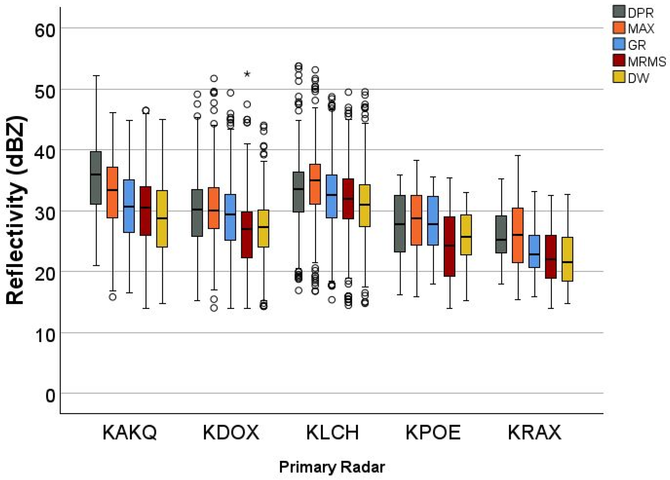
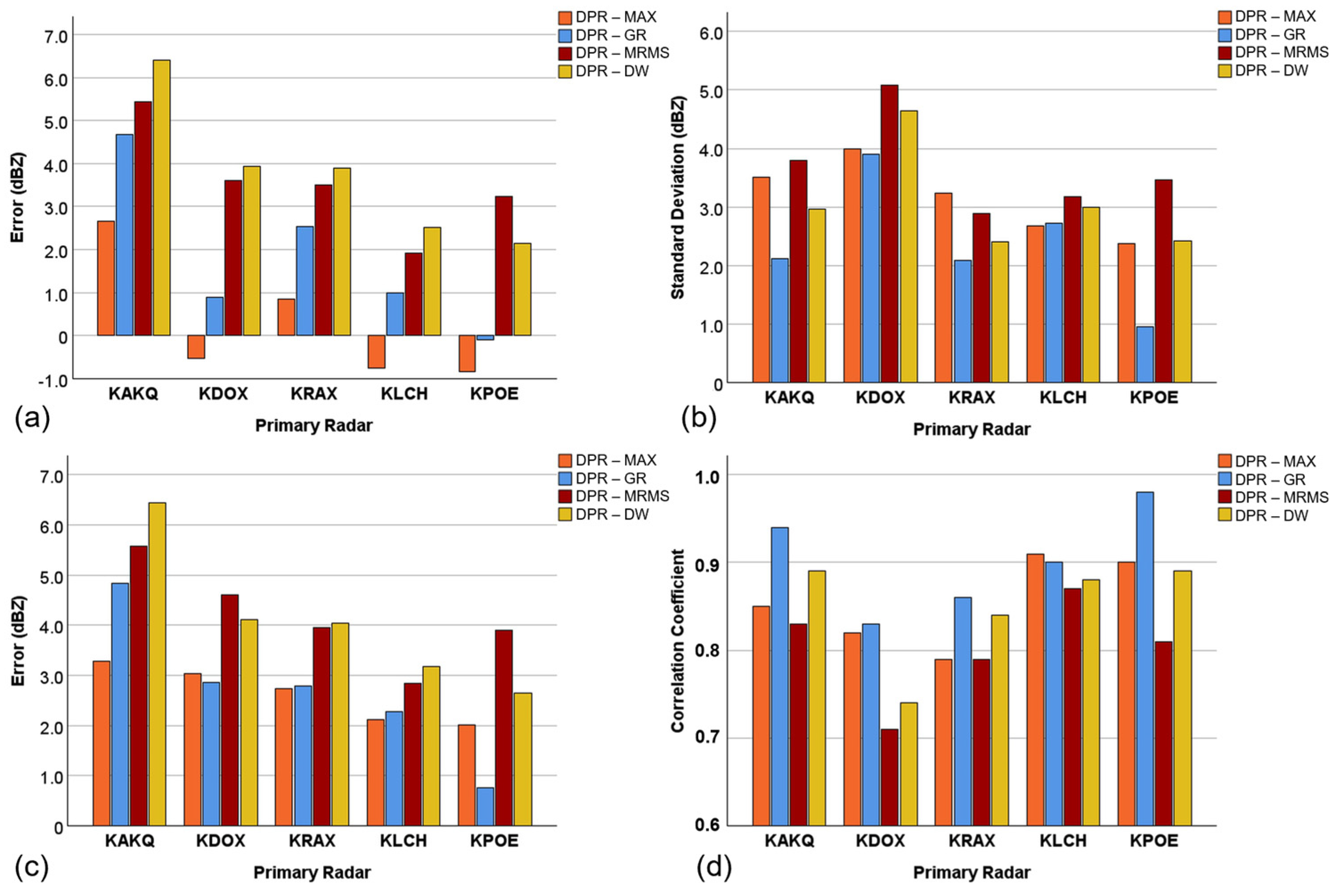
3.1. Distributions of Values and Errors

Laura and Isaias had different intensities and sizes and moved through different environmental conditions; the spatial organization of their reflectivity also differed. At Category 4 intensity, Laura was in an environment with low vertical wind shear [46] and had a closed and compact shape [47] with a ring of strong convection surrounding its northern eyewall (Figure 1a). Its rain field had a higher percentage of reflectivity values (>35 dBZ) compared to Isaias (Figure 1b). As previously mentioned, Isaias was undergoing extratropical transition at the time of the DPR overpass, a process that is associated with elongation and asymmetrical distributions of storm rainbands [47,48] with dry air entraining into the southern side of the eyewall and a broad arc of stratiform rain extending towards the northeast. Figure 1b shows the lack of reflectivity south of the center and a largely stratiform rain shield with some embedded convection extending northeast of the center.
The varying range and median reflectivity values of the sampling methods for each radar (Figure 5) supports our decision to examine data from each radar separately. The DPR detected its highest values over KAKQ (Figure 3a), with its median value nearly 2.3 dBZ higher than over KLCH, where its second-highest median value occurred. The lower reflectivity values at KAKQ for the WSR samples (Figure 3b–e and Figure 5) lead this station to have the largest range in medians (7.2 dBZ). MAX has the highest average of the ground-based samples but is 2.6 dBZ lower than DPR. Although the four WSR methods have their second-highest median values at this station, their large difference from DPR (Figure 3f–i) likely means that the null hypothesis for this Friedman test will be rejected.
The four WSR samples (MAX, GR, MRMS, DW) have their highest values at KLCH (Figure 2b–e and Figure 5), where DPR has its second-highest values (Figure 2a and Figure 5). All sampling methods have their third-highest median values at KDOX (Figure 3a–e and Figure 5). The range in median values is lowest at KDOX, spanning less than 3.25 dBZ, and second lowest at KLCH, spanning 4 dBZ. The smaller range of median values suggests that Friedman tests could be accepted at these two radars. Yet these two radars also had the most outliers in reflectivity, which are defined as values >1.5 times the interquartile range below the first quartile or above the third quartile (Figure 5). Even though the Friedman test is non-parametric, the number and spread of the outliers might make the differences in ranks large enough to reject the null hypothesis.
Overall reflectivity values are lower at KPOE (Figure 2a–e and Figure 5) and KRAX (Figure 3a–e and Figure 5) compared to the other radars. The interquartile ranges are also lower at these two radars. The range of median values is similar, at 4.5 dBZ for KRAX and 4.6 dBZ for KPOE, and without outliers, this suggests that these radars have the best chance of acceptance of the null hypothesis in the Friedman test.
Next, we check the values of mean error (Figure 6a) and its standard deviation (Figure 6b), mean absolute error (Figure 6c), and correlation coefficients (Figure 6d). Although MAX generally has the lowest mean error, mean absolute errors are similar between MAX and GR, while GR has the lowest standard deviation (Figure 6b) and highest correlation coefficients (Figure 6d); thus, GR and MAX show more similarity in reflectivity to DPR than MRMS and DW. Method DW has higher correlation coefficients than MRMS (Figure 6d), but MRMS generally has lower mean errors than DW (Figure 6a). Looking at individual radars, values are closest to DPR for MAX, GR, and DW at radar KPOE when all four metrics are considered, indicating that this radar has a good chance of acceptance of the null hypothesis in its Friedman test. For GR, the mean error is near zero (Figure 6a), and the mean absolute error is <1 (Figure 6c), indicating a closer match to DPR than the other sampling methods at this radar. As for the other radars, GR also has the best metrics at KDOX compared to the other sampling methods, while MAX has the best metrics at KRAX and KLCH.
When comparing our results from the GPM GVS VN to other studies that have utilized this database, our GR values tend to have larger differences relative to DPR. In general, mean error and mean absolute error values are higher for our GR than reported for five radars studied by [11] for events that mostly did not contain reflectivity from TCs. Their mean biases ranged from 0.18 to 0.64, MAE was 2.38–2.67 dB, and correlation coefficients were 0.87–0.9 for Ku-band. Although our correlation coefficients are in a similar range, our mean errors and mean absolute errors are farther from zero compared to theirs. A study of three radars that did not receive any TC-related precipitation [28] found biases ranging from 1.68 to 2.2 dB and standard deviation values ranging from 0.42 to 1.06 dB, while ours range from −0.1 to 4.68 and 0.95 to 3.9. They examined matchups that occurred within 120 s of radar sweep and DPR overpass to limit temporal offsets, which may explain our high standard deviation values compared to theirs as we did not employ this limitation. Additionally, [26] found that offset times of 200 s contribute to imperfect spatial matching of data due to precipitation feature advection and evolution. Given this range of findings in previous studies, we further explore temporal offsets in the next section.

3.2. Friedman Tests and Post-Hoc Dunn’s Tests

The null hypothesis is rejected in each Friedman test (Table 3). This indicates that the values of each of the five reflectivity groups at each radar are significantly different. In all five tests, MRMS and DW mean ranks are the lowest (Table 4), indicating that MRMS and DW reflectivity values are generally lower than those generated by the other three methods (e.g., Figure 5). Methods GR and DPR have similar mean ranks at KPOE, and at the other radars, DPR or MAX had the highest mean ranks. The highest overall mean rank belongs to DPR at KAKQ, as we expected, due to the higher reflectivity values (Figure 5).
We now examine the results of the post-hoc Dunn’s pairwise tests with correction factors for multiple tests. Accepting the null hypothesis means that the sampling methods produced similar results, and so these results are bolded in Table 5. Out of 50 tests, only 11 have the null hypothesis accepted, indicating that the reflectivity values produced by the five sampling methods are generally different. Results vary by radar and by the sampling methods being compared. Sampling methods are most similar at KPOE, with four of 10 tests accepting the null hypothesis, which supports the results of the metrics calculated in Figure 6. The two radars closest to the TC circulation centers where precipitation features are moving and changing the fastest (KLCH and KAKQ) are the most dissimilar among the sampling methods, with just one significant result each. The DPR and MAX sampling methods are similar to one another, retaining the null hypothesis at four of five radars, and MRMS and DW are similar at three of five radars. Sampling methods DPR and MAX are very different from MRMS and DW in all tests, as DPR and MAX produced higher values and, therefore, higher ranks than MRMS and DW (Figure 5 and Table 4). These results suggest that the weighting applied in the MRMS and DW analyses are similar and resulted in lowered reflectivity values relative to the other sampling methods. Thus, we will focus our discussion on MAX and GR.

3.3. Comparisons Between DPR and GR

The sampling methods are most similar to one another at KPOE (Table 4), which could be attributed to a few factors, including a small offset between the VCP start and DPR overpass times, only stratiform precipitation being detected, and dry conditions over and near the radar. Here, the DPR overpass occurred approximately 2 min after the start of the VCP scan (Table 2). The precipitation occurred 50–100 km away from the radar; thus, sweeps with elevations 1.3–3.1° sampled the precipitation. These three scans occurred consecutively over 80 s, which is shorter than the time span at the other four primary radars in our study. These KPOE scans also occurred within 90 s of the DPR overpass. As [28] evaluated matched points <120 s apart, this suggests that this time limit is a good threshold to achieve the best results, although their analysis used radars that did not sample TCs with their fast rotational motion. Since it is not raining over KPOE, a wet radome could not have caused attenuation here. Additionally, all KPOE precipitation is tagged as stratiform in the GPM GVS VN database, a type of rainfall that tends to have weak horizontal gradients in reflectivity. Given the 5-km footprint of DPR [33], the averaging required of WSR reflectivity to match that resolution would have incorporated more uniform values than if convective regions were included, where horizontal gradients are high. Additionally, most of the points at KPOE are outside the radius of hurricane-force winds, meaning that observed features are moving slower compared with nearby KLCH, which is located within this radius.
To provide a contrasting comparison within the same hurricane, we next discuss the results of the analysis at KLCH. Despite the apparent similarities in distributions from the boxplots at KLCH, none of the comparisons produced similar ranks here. During the VCP, a rainband is over the radar, so a wet radome could have affected reflectivity values. Also, observations occurred over the full 0–100 km range, which means that a larger number of tilts are needed to sample the storm than at KPOE. Scanning with VCP 215 (Table 2), elevations 1.36–6.44° occurred over a 195-s window with a break in the middle to return to the 0.53° elevation for a SAILS. The DPR overpass occurred within a minute of the VCP start time, but the higher tilts were not scanned for three more minutes, and the VCP took the longest of the three radars that sampled Laura (Table 2). The spatial pattern of differences reveals positive and negative values adjacent to one another for all four WSR comparisons with DPR (Figure 2f–i), which could be caused by the same feature being detected in different places as it moved. This result underscores the importance of examining the spatial patterns of the matched points (Figure 2) rather than just looking at the distribution of the data (Figure 5).
For Isaias at KDOX, DPR and GR had similar values, as did MRMS and DW (Figure 3 and Table 5). The closest matched point is 30 km away from KDOX (Figure 3 and Table 2), and thus, elevations 1.3–5.1° are key in detecting this precipitation. The VCP began about 30 s prior to the DPR overpass (Table 2), and scans that would have detected reflectivity at 3 km occurred during a 165 s window. After 1.32°, three SAILS at 0.49° occurred before moving onto 1.8°. All precipitation is >230 km from the storm center and beyond the radius of gale-force winds, so tangential motion is relatively slow compared to the other primary radars. However, the storm’s fast-forward speed (top 8% of Atlantic cases at the time of landfall) could still allow precipitation to shift enough to be detected by different beams between scans. Similar to the results at KLCH, the alternating pattern of red and blue points for KDOX (Figure 3f–i) in all WSR comparisons is suggestive of these shifts. However, a large area of stratiform precipitation west of the radar (Figure 3a–e) had weak gradients in reflectivity, meaning that delays in consecutive scans would not cause as large of a difference in values as would occur in convective regions. It is likely that the good match in this area (Figure 3f–i) supported an overall better match between the GR and the DPR. In fact, 86% of points are stratiform at KDOX, which had an average difference of 0.54 dBZ between DPR and GR, compared to a 2.94 dBZ difference for points labeled by NASA as convective. Despite a relatively large temporal offset between the DPR overpass and GR scans coupled with relatively fast storm motion, the presence of mainly stratiform precipitation, and possibly the lack of wet radome (Table 2), could explain why DPR and GR matched better here than at other radars.
At KRAX and KAKQ, GR values are much lower compared to DPR and are a close match to those from MRMS rather than DPR. We discuss KRAX first, as all sampling methods produced their lowest overall reflectivity values (Figure 5) and lowest standard deviation of values (Figure 6b) in this analysis. The lower values recorded by all sampling methods are likely due to the eroding outer edge of the storm containing mostly stratiform precipitation as dry air entrained into the core due to baroclinic forcing from a mid-latitude trough [31]. The long duration and pattern of SAILS could have led to a poorer match between DPR and GR. The volume scan took the longest at KRAX (Table 2), with an elevation of 19.4° being scanned 7 min after the start time. There are four SAILS at 0.21° or 0.22° dispersed throughout the period so that the entire volume scan took longer than it did when these extra scans are sequential as they are at KDOX. Tilting down and up repeatedly also caused temporal gaps between the scans at higher elevations, allowing more time for features to move and/or change between spatially adjacent scans. The discontinuities resulting from this scan pattern could help explain why GR and MRMS had more consistent reflectivity values, but neither resembled DPR.
One explanation for the varied results among the radars is where each radar is in its pattern of sweeps when the DPR passes overhead relative to where precipitation is located within the range of the radar. Because the match-up between DPR and GR only included points sampled within 100 km of each radar and all radars used VCP 212 or 215 (Table 6), only elevation scans 1.3° and higher provide data at 3 km altitude [20] (their Figure 1), and so we focus on these scans to contextualize the GR analysis. We know that the GR points come from that radar. The distance weights used in method DW assure that the closest radar’s data are included in the mosaic when the analysis only considers observations within 100 km of a radar. Precise details of the calculations for the MRMS mosaics are not available, but we assume, given similarities with DW, that a distance-weighting scheme is employed. However, the documentation does not allow us to know whether and how neighboring radars may influence the value of a grid cell in the MRMS mosaic. That said, MAX observations can come from lower-elevation scans of neighboring radars. Since VCPs start at the lowest scan angle, this means that data from a larger range of times relative to the DPR overpass could have been incorporated into each MAX mosaic. Given that MAX mosaics utilized multiple radars while GR did not, we will discuss GR results next and MAX results in Section 3.4.
At radar KAKQ, Figure 5 shows that DPR had higher reflectivity values than WSRs, which is confirmed by having the highest average rank across all tests (Table 4). Most WSR values are well below those detected by DPR; only 4%, 6%, and 1% are GR > DPR (Figure 3g), MRMS > DPR (Figure 3h), or DW > DPR (Figure 3i), respectively. The VCP took the longest of the 10 radars (Table 2). As at KRAX, the discontinuities resulting from this pattern of scans could explain why GR and MRMS are similar at KAKQ. However, an offset in the timing of detection is likely not the main reason for having such low values across all WSR sampling methods, as a timing offset would produce a mix of positive and negative differences as we see in other radars (e.g., Figure 3g for KDOX). Instead, the results suggest that the power is low, although we cannot pinpoint its precise cause. KAKQ is the closest radar to the center of Isaias, and the edge of the deteriorating eyewall is producing precipitation over this radar (Figure 1), which supports the decreases due to attenuation via wet radome. It is also possible that a drift in calibration was causing KAKQ to “run cold”, emitting less power than when calibration is ideal, which in turn means lower reflectivity is returned.

3.4. Results for MAX Mosaic

The pairwise tests revealed that keeping the maximum reflectivity value when creating a mosaic produced values similar to DPR at four of the five radars, more than any other WSR method, as only one comparison between DPR and GR was similar, while all tests showed dissimilarities between DPR and MRMS and DPR and DW. Thus, keeping the highest value when multiple values are present rather than weighting and/or averaging produces values that are generally closer to DPR. Additionally, in the analysis of each primary radar, at least two secondary radars contributed values to the MAX mosaic (Figure 7), and none of the five primary radars had more than half of their values used in the creation of a mosaic. This suggests that it can be advantageous to allow neighboring radars an equal chance to contribute to a mosaic rather than weighing values so that the closest radar is prioritized. A disadvantage of the MAX sampling method is that a region can be sampled more than once if enough time passes between scans by neighboring radars and that the same region would move into a different grid cell. This “oversampling” could explain the higher percent of DPR < MAX observations (40%) compared to the other sampling methods (Figure 2 and Figure 3), as these oversampled regions could be just below the value of DPR if sampled with a small temporal offset by one radar, but then larger than DPR if sampled before or after the DPR overpass when that region was experiencing lower reflectivity at the time of DPR overpass. For Laura, radar KHGX contributed about a third of the observations, and 61% of these observations had DPR < MAX (Figure 7). By contrast, only 20% of observations contributed by KLWX to the Isaias mosaic featured DPR < MAX, which was the highest for that TC (Figure 7).
Given the strong contribution of KHGX to the analysis at KLCH and KPOE (Figure 7) and the large percentage of DPR < MAX at these locations, we explore this secondary radar further. More specifically, KHGX contributed half of the observations where DPR < MAX for KPOE’s observations, with an average difference of −2.9 dBZ, with negative meaning MAX is higher. For the KLCH analysis, KHGX contributed 31% of observations where DPR < MAX had an average difference of −2.55 dBZ. Radar KHGX contributed to observations 100–220 km away from its location (Table 2), meaning that scan elevations 0.46–1.28° detected the precipitation at 3 km. It has the earliest VCP start time for the Laura mosaic (Table 2), and there are three SAILS in addition to scans at 0.85° and 1.28° over approximately three minutes. This is 3–6 min earlier than the higher elevation scans that would have produced data near the radar in the scans of KLCH. This large window of time, coupled with the fast-moving precipitation regions around the center of a major hurricane, facilitates the movement of features across neighboring grid cells between scans, potentially sampling convective regions twice.
As KHGX contributed numerous values that are too high compared to DPR, we create another MAX mosaic for Laura using only KLCH and KPOE and then compare the map of differences to the original (Figure 2 and Figure 8). At KLCH, the mean error reduces to −0.1 dBZ with a similar standard deviation (2.71 dBZ) and MAE (2.02 dBZ). At POE, a larger improvement occurs with a mean error of 0.33 dBZ, standard deviation of 1.81 dBZ, and MAE of 1.41 dBZ. The correlation coefficient is the same for KLCH (0.91) but improves to 0.94 for KPOE. Differences are smaller as well in the new MAX mosaic comprised of only KLCH and KPOE (Figure 8a vs. Figure 8b), where most values are at or below 2 dBZ, although alternating patterns of red and blue suggest movement over the grid between scans even in this narrower timeframe since KLCH and KPOE began their VCPs within 70 s of each other while KHGX had started earlier (Table 2). The reduction in blue colors overall, indicating that MAX was closer to DPR in the new mosaic, particularly on the western side, suggests that the removal of KHGX improved the match between WSR and DPR. This result indicates that it could be advantageous for a researcher to create their own mosaic to manually exclude radars that could be scanning at different times, experiencing wet radome, and/or running hot or cold.
As reflectivity at KAKQ is so much lower than DPR in the other ground-based sampling methods, it is not surprising that it contributed the least to any MAX mosaic (Figure 7). The largest contribution for the KAKQ region came from KRAX. The DPR detected reflectivity between 08:52:30 and 08:53:00 UTC over this region. Even though KRAX was using VCP 212 (Table 2), its lowest scan angle was 0.21°, and it completed three scans at this elevation between 08:50:32 and 08:53:56 UTC. There was also a scan at 0.92° degrees at 08:52:35 UTC covering the region south of radar KAKQ as the DPR flew overhead. This lower scan elevation would allow the beam to travel farther at lower altitudes, thus enabling it to detect precipitation at 3 km AGL at a farther distance than other radars. In fact, KRAX has the most points in the Isaias MAX analysis, 1.5 times more than the next closest contributors of KDOX and KLWX (Figure 7). The MAX mosaic uses much more data from neighboring radars, especially KRAX and KLWX, for the region within 100 km of primary radar KAKQ than from KAKQ, and this explains why the values in the MAX dataset are much closer to the distribution of DPR than GR, which only utilized data from KAKQ.

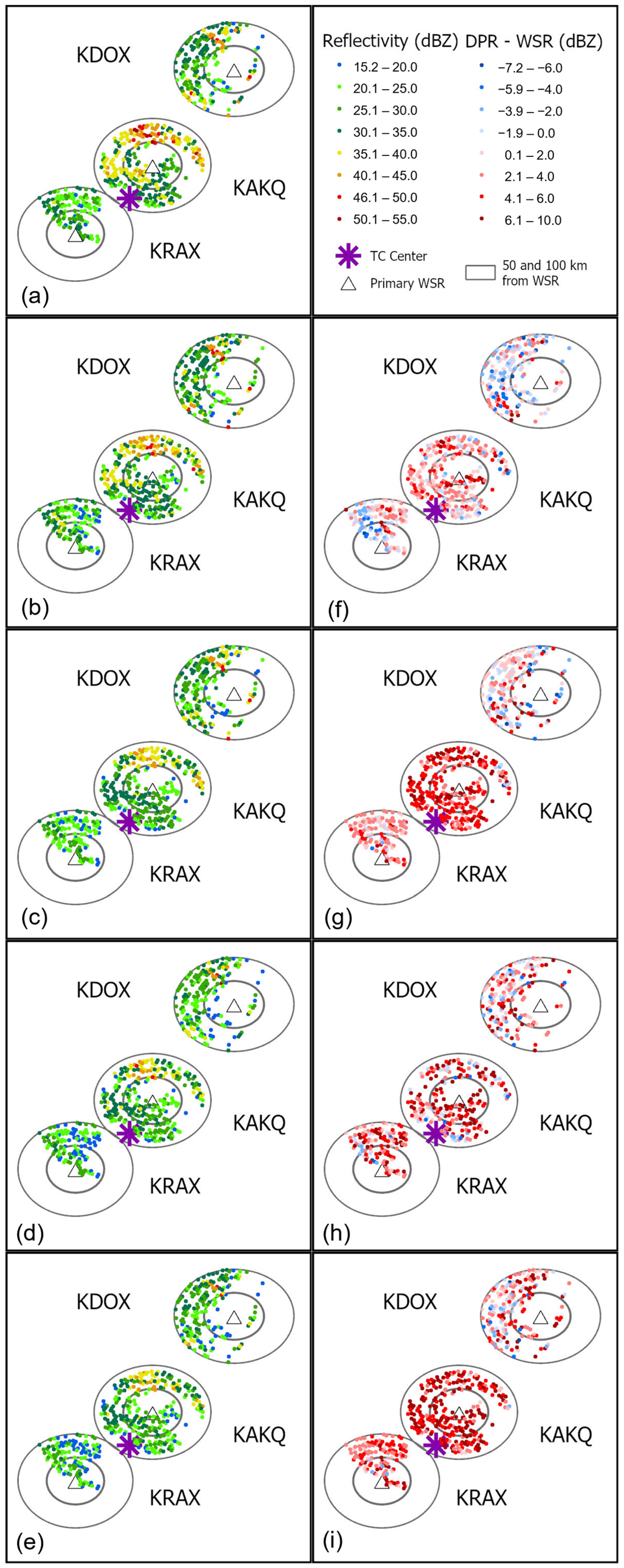
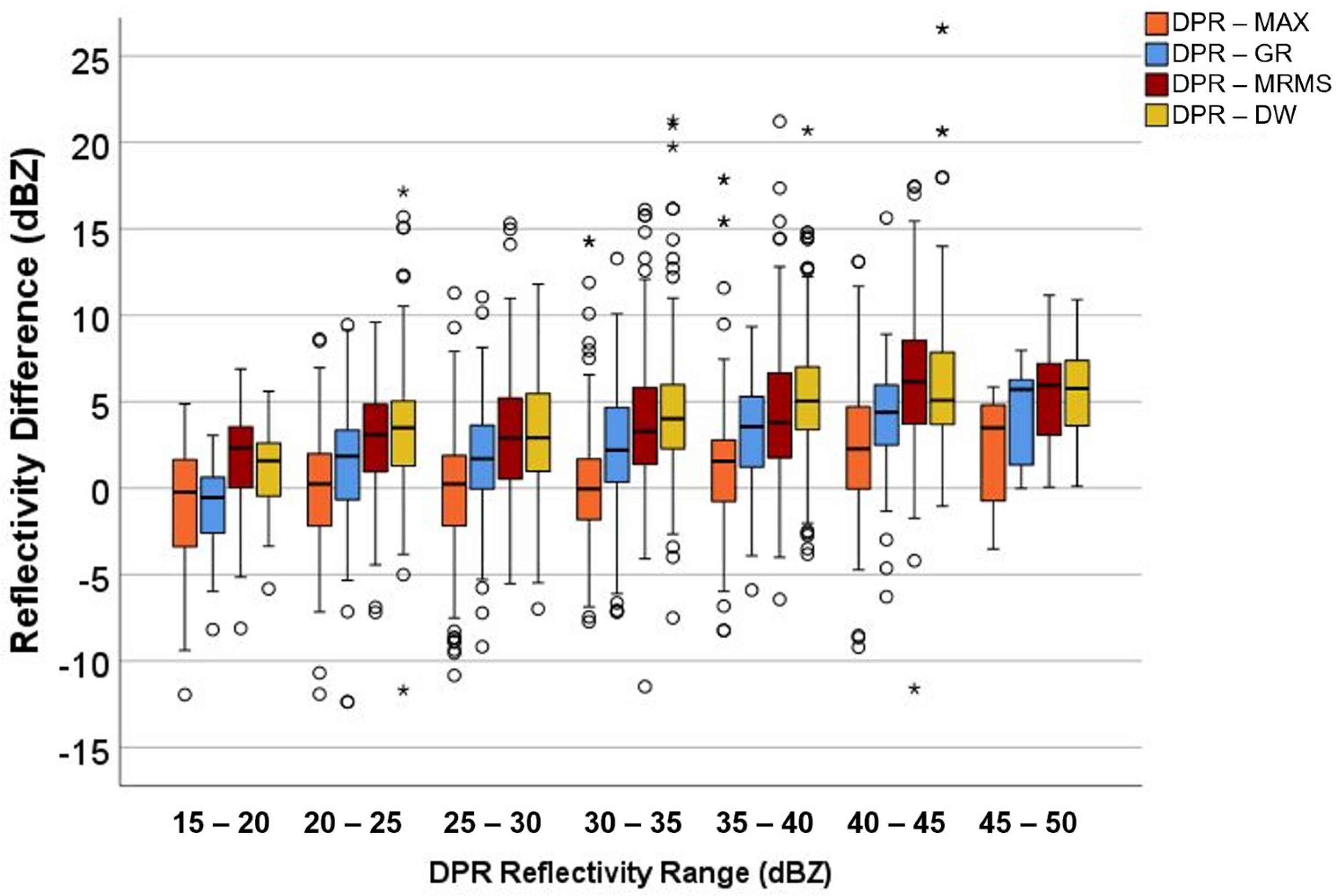
3.5. Trends in Difference Values According to DPR Reflectivity

When we examine the differences between DPR and the WSR-based sampling methods according to DPR value groups, we find evidence of an increasing trend in the differences as DPR reflectivity increases. Tests are statistically significant at the 95% level for all four WSR groups when binned in 5 and 3 dBZ intervals; thus, we only show results for the 5 dBZ bin analysis (Table 6). However, when examining the distribution of data in a boxplot, we notice a different pattern for MAX compared to the other methods (Figure 9). The median value for MAX is around 0 dBZ from 15–20 to 30–35 dBZ and increases to about 4 dBZ at 45–50 dBZ. For the other sampling methods, there is a general upward trend from near zero difference in the lowest 15–20 dBZ category to biases greater than 5 dBZ in the highest 45–50 dBZ category. At 35–40 dBZ, the mean difference in MAX is similar to that of GR at 20–25 dBZ. A similar pattern occurred in the analysis arranged in 3 dBZ bins, with the trend in MAX errors appearing to change from nearly flat to increasing after the 32–34 dBZ group. To evaluate whether the difference for the lower reflectivity values was not increasing for MAX as it was in the other three sampling methods, we again performed sets of the Jonckheere-Terpstra test by only considering the first four groups of the 5-dBZ binned groups and the first five groups of the 3-dBZ-binned analysis. Thus, DPR values are less than 35 and 34 dBZ in these analyses. As before, results are similar for the 5 and 3-dBZ binned groups, so we focus on the 5 dBZ results. Here, we find that, indeed, the null hypothesis is accepted for the MAX analysis, indicating a lack of increasing trend, while the null hypothesis continues to be rejected for the other three sampling methods. These results also suggest that allowing scans from other radars and/or retaining the highest value when multiple values exist in a grid cell produces a better and more consistent match to DPR values in the lower reflectivity values. However, even retaining the highest value among all radars cannot match the DPR values in higher reflectivity regions where gradients tend to be stronger, and features change at a faster rate.

3.6. Exploring Time Offsets

To give context on how much a two-minute difference can make in a mosaic, we enter MRMS values into Friedman tests. Differences as small as two minutes could be apparent given the results of previous research and the fact that rapidly changing reflectivity patterns occur in the TC’s core, as previously discussed. Thus, we examine differences in ranks for five mosaics created two minutes apart so that the first and last are eight minutes apart. As none of the VCPs lasted 8 min (Table 2), the mosaics created eight minutes apart feature different VCPs at all radars, therefore having the highest chance of being dissimilar. The results of the closer time offsets could be influenced by when radars started their scans to bring new data into the mosaic. We center the analysis on the MRMS timestamp closest to the DPR overpass, thus 0300 (0852) UTC for Laura (Isaias), analyzing mosaics at 0256, 0258, 0300, 0302, and 0304 (0848, 0850, 0852, 0854, and 0856) UTC.
We find that the null hypothesis is accepted (similar reflectivity values) at the three Isaias radars. This result could be due to the staggered nature with which the new VCPs began over the eight minutes and the fact that the predominantly stratiform regions sampled in the analysis are not changing as rapidly. However, it is rejected at the two radars that sampled regions within the radius of gale-force and hurricane-force winds in Hurricane Laura (Table 5). Post-hoc Dunn’s tests when the Bonferroni-corrected alpha value of 0.005 is applied (as ten comparisons are made in each family of tests) (Table 7) reveal that values are similar when mosaics are only two minutes apart and mostly similar when four minutes apart. The exception for the four-minute comparison occurred during the tests of mosaics with timestamps of 0256 UTC and 0300 UTC. The test for KLCH is accepted, although just barely, while the test is rejected for KPOE. The fact that a new VCP began for KPOE in the middle of this period while it occurred at the end for KLCH (Table 2) could account for this slight difference, although we cannot confirm as the details of the MRMS mosaicking strategy are not available.
Tests at six- and eight-minute offsets showed that the values are different, as we expected. We also note that reflectivity values are consistently lower for MRMS than GR, MAX, and DPR. As a result, any averaging that occurs while creating the mosaic may smooth the differences from one period to the next, which could help explain why a shorter offset, such as two minutes suggested by [28], did not produce a significant difference in our study and only one comparison less than the 200 s suggested by [26] produced significant differences. It also underscores the need for more analyses of hurricanes to further explore differences as the tangential wind fields vary outwards from the circulation center and are detected by radars with varying VCP durations.

4. Conclusions

This study compared reflectivity values derived from space-based (DPR) and multiple ground-based (WSR) radars that scanned the rain fields of two landfalling TCs. It is important to examine how TC rain fields are observed by multiple ground-based radars given their mix of stratiform and convective clouds and varying tangential wind speeds that circulate rainfall regions around the storm center as well as rapid changes in structure can cause issues while neighboring ground-based radars scan in different patterns for different durations. The novelty of our study lies in its focus on TCs and the use of the DPR to compare multiple mosaicked reflectivity datasets from ground-based radars. More specifically, ground-based radar values were derived via four sampling methods, including a precise spatial and temporal matching technique within 100 km of each radar (GR) and three mosaics created at timestamps of the closest match and with data points extracted from the mosaics at the same latitude and longitude as the GR points but at constant altitude. These mosaics were the MRMS plus two mosaics we created by using a distance-weighted average (DW) and by retaining the maximum value (MAX) when grid cells have more than one reflectivity value. Rainband configurations and tangential and forward velocities differed between the two TCs, as Laura was a major hurricane at its maximum intensity during the DPR overpass, while Isaias was a weakening tropical storm beginning to transition into an extratropical cyclone. The goals were to (1) use DPR as a baseline to compare four methods of sampling reflectivity from ground-based radars (WSR) and (2) explore which factors affected the goodness of the match between DPR and each WSR sampling method.
The sampling method that produced values with the closest match to DPR was MAX, or retaining the maximum reflectivity value when creating a single-station and multi-radar mosaic. This method allowed data from neighboring radars to be equally considered in the mosaic rather than the distance-weighting methods that give preference to the closest radar before averaging values. Retaining the maximum value is advantageous when neighboring radars might be running “cold” or have attenuation due to wet radome or drifts in calibration, issues that have been reported in other studies. The disadvantage of retaining the maximum value is that a region of high reflectivity could be sampled by both radars at different times and locations and, therefore, be double-counted in the mosaic. In contrast, the distance weight (DW) mosaic and MRMS produced similar values when compared to one another and much lower reflectivity values compared to DPR and MAX. Previous studies suggested that a time offset of less than 120 s is preferable (e.g., [28]), and our results support this finding, especially given the fast tangential motion and changes to convective clouds occurring in the core of a major hurricane.
In addition to temporal offsets, the differences between DPR and WSR values also varied by DPR reflectivity. Stratiform observations yielded smaller differences, which could be due to weaker reflectivity gradients, meaning that the averaging of the GR data under the DPR footprint might be more representative of the actual values (lower standard deviation) and/or that the stratiform regions are not changing as rapidly. Convective clouds located farther from the WSR may not be sampled by multiple beams; thus, their horizontal gradients in reflectivity are not detected. Also, the fast motions in some parts of the TC could mean those features are sampled at different times, producing both positive and negative difference values when DPR is compared to WSR. Retaining the maximum value helps reduce differences with DPR from 15–35 dBZ, but differences increase from 35–45 dBZ even in the MAX observations, whereas differences were larger and increased gradually in the other sampling methods.
This study examined two contrasting TC landfalls where the TCs were sampled by multiple radars, but adding more cases to evaluate the generalizability of these results is necessary. For example, examining a larger number of radars where rain is occurring over the instrument could support the explanation of wet radome for lowering a radar’s values relative to its neighbors where rain is not occurring on site. More cases would permit a sensitivity analysis for time offsets between neighboring radars and their detection of precipitation regions moving at different forward and tangential speeds. Exploring more instances where multiple radars are detecting the same precipitation and manually setting which radars enter the mosaic, as in our KHGX example, could also help establish the methodology to derive the most spatially accurate representation of TC rain fields. A more detailed spatial analysis of a larger sample of difference values in regions scanned by multiple radars, such as a hot spot analysis, could yield additional information about radars that tend to have higher or lower values than their neighbors. Finally, including cases with more convective regions would permit further exploration into the differences in the detection of stratiform and convective cases by the DPR and WSR units.

Author Contributions

Conceptualization, C.J.M.; methodology, C.J.M.; formal analysis, C.J.M.; data acquisition, C.J.M. and K.M.W.; writing—original draft preparation, C.J.M.; writing—review and editing, S.E.Z. and K.M.W.; visualization, C.J.M.; funding acquisition, C.J.M., S.E.Z. and K.M.W. All authors have read and agreed to the published version of the manuscript.

Funding

This research was funded by the National Science Foundation (grant numbers AGS-2012008, AGS-2011981, and AGS-2011812). The APC was waived.

Data Availability Statement

All data were obtained from publicly available datasets, including IBTrACS: https://www.ncei.noaa.gov/products/international-best-track-archive, accessed on 7 April 2022; The GPM Ground Validation Data Archive: https://gpm-gv.gsfc.nasa.gov/; accessed on 7 July 2021 MRMS: https://mesonet.agron.iastate.edu/archive/, accessed on 27 August 2020; WSR-88D Level II archive: https://registry.opendata.aws/noaa-nexrad, accessed on 2 December 2023. The code used to perform the mosaic analysis was downloaded from https://github.com/striges, accessed on 1 September 2019.

Acknowledgments

We thank the anonymous reviewers for their helpful suggestions that improved this manuscript.

Conflicts of Interest

The authors declare no conflicts of interest. The funders had no role in the design of the study; in the collection, analyses, or interpretation of data; in the writing of the manuscript; or in the decision to publish the results.

References

  1. Crum, T.D.; Alberty, R.L. The WSR-88D and the WSR-88D operational support facility. Bull. Am. Meteor. Soc. 1993, 74, 1669–1688. [Google Scholar] [CrossRef]
  2. Lakshmanan, V.; Smith, T.; Hondl, K.; Stumpf, G.J.; Witt, A. A real-time, three-dimensional, rapidly updating, heterogeneous radar merger technique for reflectivity, velocity, and derived products. Weather. Forecast. 2006, 21, 802–823. [Google Scholar] [CrossRef]
  3. Melnikov, V.M.; Zrnić, D.S.; Doviak, R.J.; Chilson, P.B.; Mechem, D.B.; Kogan, Y.L. Prospects of the WSR-88D radar for cloud studies. J. Appl. Meteorol. Climatol. 2011, 50, 859–872. [Google Scholar]
  4. Ryzhkov, A.; Zrnic, D.S. Precipitation and attenuation measurements at a 10-Cm wavelength. J. Appl. Meteor. 1995, 34, 2121–2134. [Google Scholar] [CrossRef]
  5. Mancini, A.; Lebrón, R.M.; Salazar, J.L. The Impact of a wet S-Band radome on dual-polarized phased-array radar system performance. IEEE Trans. Antennas Propag. 2018, 67, 207–220. [Google Scholar] [CrossRef]
  6. Parry, C.; Fenn, A.J.; Morris, A.; Thomas, H. Analysis and mitigation of the reflected power on an S-band planar phased array antenna transmitting in a wet spherical radome. In Proceedings of the 2022 IEEE International Symposium on Phased Array Systems & Technology (PAST), Waltham, MA, USA, 11–14 October 2022; pp. 1–7. [Google Scholar]
  7. Smith, J.A.; Seo, D.J.; Baeck, M.L.; Hudlow, M.D. An intercomparison study of NEXRAD precipitation estimates. Water Resour. Res. 1996, 32, 2035–2045. [Google Scholar]
  8. Ulbrich, C.W.; Lee, L.G. Rainfall measurement error by WSR-88d radars due to variations in Z-R law parameters and the radar constant. J. Atmos. Ocean. Technol. 1999, 16, 1017–1024. [Google Scholar]
  9. Matyas, C.J. Use of ground-based radar for climate-scale studies of weather and rainfall. Geogr. Compass 2010, 4, 1218–1237. [Google Scholar]
  10. Schwaller, M.; Morris, K. Satellite observations for calibration of ground radar networks. In Proceedings of the AGU Fall Meeting Abstracts, San Francisco, CA, USA, 5–9 December 2011. H41G-1135. [Google Scholar]
  11. Biswas, S.K.; Chandrasekar, V. Cross-validation of observations between the GPM dual-frequency precipitation radar and ground based dual-polarization radars. Remote Sens. 2018, 10, 1773. [Google Scholar] [CrossRef]
  12. Matyas, C.J.; Zick, S.E.; Tang, J. Using an object-based approach to quantify the spatial structure of reflectivity regions in Hurricane Isabel (2003): Part I: Comparisons between radar observations and model simulations. Mon. Wea. Rev. 2018, 146, 1319–1340. [Google Scholar] [CrossRef]
  13. Matyas, C.; Tang, J. Measuring radial and tangential changes in tropical cyclone rain fields using metrics of dispersion and closure. Adv. Meteorol. 2019, 2019, 8613943. [Google Scholar] [CrossRef]
  14. Sun, M.; Wang, H.; Li, Z.; Gao, M.; Xu, Z.; Li, J. Study on reflectivity data interpolation and mosaics for multiple Doppler weather radars. EURASIP J. Wirel. Commun. Netw. 2019, 2019, 145. [Google Scholar] [CrossRef]
  15. Brook, J.P.; Protat, A.; Soderholm, J.S.; Warren, R.A.; McGowan, H. A variational interpolation method for gridding weather radar data. J. Atmos. Ocean. Technol. 2022, 39, 1633–1654. [Google Scholar] [CrossRef]
  16. Yuter, S.E.; Houze, R.A. Three-Dimensional kinematic and microphysical evolution of Florida cumulonimbus. Part I: Spatial distribution of updrafts, downdrafts, and precipitation. Mon. Wea. Rev. 1995, 123, 1921–1940. [Google Scholar] [CrossRef]
  17. Langston, C.; Zhang, J.; Howard, K. Four-Dimensional dynamic radar mosaic. J. Atmos. Ocean. Technol. 2007, 24, 776–790. [Google Scholar] [CrossRef]
  18. Zhang, J.; Howard, K.; Gourley, J.J. Constructing three-dimensional multiple-radar reflectivity mosaics: Examples of convective storms and stratiform rain echoes. J. Atmos. Ocean. Technol. 2005, 22, 30–42. [Google Scholar] [CrossRef]
  19. OFCM. Federal Meteorological Handbook, No. 11: WSR-88D Meteorological Observations. In Part C WSR-88D Products and Algorithms; Office of the Federal Coordinator for Meteorological Services and Supporting Research, Ed.; U.S. Department of Commerce/NOAA: Silver Spring, MD, USA, 2017. [Google Scholar]
  20. Kingfield, D.M.; French, M.M. The influence of WSR-88D intra-volume scanning strategies on thunderstorm observations and warnings in the dual-polarization radar era: 2011–20. Weather. Forecast. 2022, 37, 283–301. [Google Scholar] [CrossRef]
  21. Matyas, C.J. Associations between the size of hurricane rain fields at landfall and their surrounding environments. Meteorol. Atmos. Phys. 2010, 106, 135–148. [Google Scholar] [CrossRef]
  22. Willoughby, H.E.; Marks, F.D.; Feinberg, R.J. Stationary and moving convective bands in hurricanes. J. Atmos. Sci. 1984, 41, 3189–3211. [Google Scholar] [CrossRef]
  23. Anagnostou, E.N.; Morales, C.A.; Dinku, T. The use of TRMM precipitation radar observations in determining ground radar calibration biases. J. Atmos. Ocean. Technol. 2001, 18, 616–628. [Google Scholar] [CrossRef]
  24. Li, Z.; Wen, Y.; Liao, L.; Wolff, D.; Meneghini, R.; Schuur, T. Joint collaboration on comparing NOAA’s ground-based weather radar and NASA–JAXA’s spaceborne radar. Bull. Amer. Meteor. Soc. 2023, 104, E1435–E1451. [Google Scholar] [CrossRef]
  25. Schwaller, M.R.; Morris, K.R. A ground validation network for the global precipitation measurement mission. J. Atmos. Ocean. Technol. 2011, 28, 301–319. [Google Scholar] [CrossRef]
  26. Warren, R.A.; Protat, A.; Siems, S.T.; Ramsay, H.A.; Louf, V.; Manton, M.J.; Kane, T.A. Calibrating ground-based radars against TRMM and GPM. J. Atmos. Ocean. Technol. 2018, 35, 323–346. [Google Scholar] [CrossRef]
  27. Masaki, T.; Iguchi, T.; Kanemaru, K.; Furukawa, K.; Yoshida, N.; Kubota, T.; Oki, R. Calibration of the Dual-Frequency Precipitation Radar Onboard the Global Precipitation Measurement Core Observatory. IEEE Trans. Geosci. Remote Sens. 2020, 60, 5100116. [Google Scholar] [CrossRef]
  28. Keem, M.; Seo, B.-C.; Krajewski, W.F.; Morris, K.R. Inter-comparison of reflectivity measurements between GPM DPR and NEXRAD radars. Atmos. Res. 2019, 226, 49–65. [Google Scholar] [CrossRef]
  29. Knapp, K.R.; Diamond, H.J.; Kossin, J.P.; Kruk, M.C.; Schreck, C.J.I. International Best Track Archive for Climate Stewardship (IBTrACS); National Centers for Environmental Information: Asheville, NC, USA, 2018. [CrossRef]
  30. National Hurricane Center Tropical Cyclone Report: Hurricane Laura. National Hurricane Center, 2021. Available online: https://www.nhc.noaa.gov/data/tcr/AL132020_Laura.pdf (accessed on 28 November 2024).
  31. National Hurricane Center Tropical Cyclone Report: Hurricane Isaias. National Hurricane Center, 2021. Available online: https://www.nhc.noaa.gov/data/tcr/AL092020_Isaias.pdf (accessed on 30 November 2024).
  32. Skofronick-Jackson, G.; Berg, W.; Kidd, C.; Kirschbaum, D.B.; Petersen, W.A.; Huffman, G.J.; Takayabu, Y.N. Global Precipitation Measurement (GPM): Unified precipitation estimation from space. In Remote Sensing of Clouds and Precipitation; Andronache, C., Ed.; Springer International Publishing: Cham, Switzerland, 2018; pp. 175–193. [Google Scholar] [CrossRef]
  33. NASA/JAXA. Precipitation Measurement Missions: Global Precipitation Mission (GPM) Ground Validation System. 2015. Available online: https://gpm.nasa.gov/sites/default/files/document_files/Val_Network_Users_Guide_Vol_2_Nov2015.pdf (accessed on 25 October 2024).
  34. Iguchi, T.; Seto, S.; Meneghini, R.; Yoshida, N.; Awaka, J.; Le, M.; Chandrasekar, V.; Kubota, T. GPM/DPR Level-2 Algorithm Theoretical Basis Document; NASA Goddard Space Flight Center: Greenbelt, MD, USA, 2010. [Google Scholar]
  35. Lakshmanan, V.; Humphrey, T.W. A MapReduce technique to mosaic continental-scale weather radar data in real-time. IEEE J. Sel. Top. Appl. Earth Obs. Remote Sens. 2014, 7, 721–732. [Google Scholar] [CrossRef]
  36. Tang, J.; Matyas, C.J. High efficiency weather radar mosaic image generation framework. In Proceedings of the 2021 IEEE International Geoscience and Remote Sensing Symposium IGARSS, Brussels, Belgium, 11–16 July 2021; pp. 367–369. [Google Scholar]
  37. Tang, J.; Matyas, C.J. Fast playback framework for analysis of ground-based Doppler radar observations using Map-Reduce technology. J. Atmos. Ocean. Technol. 2016, 33, 621–634. [Google Scholar] [CrossRef]
  38. Wilks, D.S. Statistical Methods in the Atmospheric Sciences; Academic Press: San Diego, CA, USA, 1995; p. 467. [Google Scholar]
  39. Friedman, M. The use of ranks to avoid the assumption of normality implicit in the analysis of variance. J. Am. Stat. Assoc. 1937, 32, 675–701. [Google Scholar] [CrossRef]
  40. Keselman, H.; Algina, J.; Kowalchuk, R.K. The analysis of repeated measures designs: A review. Br. J. Math. Stat. Psychol. 2001, 54, 1–20. [Google Scholar] [CrossRef]
  41. Pereira, D.G.; Afonso, A.; Medeiros, F.M. Overview of Friedman’s test and post-hoc analysis. Commun. Stat.-Simul. Comput. 2015, 44, 2636–2653. [Google Scholar] [CrossRef]
  42. Dunn, O.J. Multiple comparisons among means. J. Am. Stat. Assoc. 1961, 56, 52–64. [Google Scholar] [CrossRef]
  43. Cabin, R.J.; Mitchell, R.J. To Bonferroni or not to Bonferroni: When and how are the questions. Bull. Ecol. Soc. Am. 2000, 81, 246–248. [Google Scholar]
  44. Liao, L.; Meneghini, R. GPM DPR retrievals: Algorithm, evaluation, and validation. Remote Sens. 2022, 14, 843. [Google Scholar] [CrossRef]
  45. Jonckheere, A.R. A distribution-free k-sample test against ordered alternatives. Biometrika 1954, 41, 133–145. [Google Scholar] [CrossRef]
  46. Brauer, N.S.; Alford, A.A.; Waugh, S.M.; Biggerstaff, M.I.; Carrie, G.D.; Kirstetter, P.E.; Basara, J.B.; Dawson, D.T.; Elmore, K.L.; Stevenson, J. Hurricane Laura (2020): A comparison of drop size distribution moments using ground and radar remote sensing retrieval methods. J. Geophys. Res. Atmos. 2022, 127, e2021JD035845. [Google Scholar] [CrossRef]
  47. Stackhouse, S.D.; Zick, S.E.; Matyas, C.J.; Wood, K.M.; Hazelton, A.T.; Alaka Jr, G.J. Evaluation of experimental high-resolution model forecasts of tropical cyclone precipitation using object-based metrics. Weather. Forecast. 2023, 38, 2111–2134. [Google Scholar] [CrossRef]
  48. Zick, S.E.; Matyas, C.J. A shape metric methodology for studying the evolving geometries of synoptic-scale precipitation patterns in tropical cyclones. Ann. Assoc. Am. Geogr. 2016, 106, 1217–1235. [Google Scholar] [CrossRef]
Figure 1. Reflectivity values produced during the MAX sampling method (maximum value is retained) (shading) and circles denoting locations where data are available for Dual-Frequency Precipitation Radar (DPR) and Ground Radar (GR) in the Global Precipitation Measurement Mission Ground Validation System Validation Network (GPM GVS VN) database for (a) Laura and (b) Isaias.
Atmosphere 16 00307 g001
Figure 2. Hurricane Laura reflectivity data from sampling methods (a) DPR, (b) MAX, (c) GR, (d) MRMS, and (e) DW, and the difference of each sampling method subtracted from DPR (f) MAX, (g) GR, (h) MRMS, and (i) DW.
Atmosphere 16 00307 g002
Figure 3. Tropical Storm Isaias reflectivity data from sampling methods (a) DPR, (b) MAX, (c) GR, (d) MRMS, and (e) DW, and the difference of each sampling method subtracted from DPR (f) MAX, (g) GR, (h) MRMS, and (i) DW.
Atmosphere 16 00307 g003
Figure 4. Flowchart showing the procedure for processing reflectivity from a single radar and then placing those data on the TC-centric grid. The “identify final value” step varies by approach, and the same approach is used for all single-station grids and the TC-centered grid: it either computes the distance-weighted average for the DW method or retains the maximum value for the MAX method.
Atmosphere 16 00307 g004
Figure 5. Distribution of reflectivity at each primary radar from each sampling method. Circles and asterisks denote minimum and maximum values that are outliers, whiskers denote minimum and maximum values that are not outliers, and boxes show lower and upper quartiles and median reflectivity.
Atmosphere 16 00307 g005
Figure 6. For each primary radar, each WSR sampling method is subtracted from DPR, and these statistics are portrayed as follows: (a) mean error, (b) standard deviation of the mean error, and (c) mean absolute error. (d) Correlation coefficients calculated between DPR and each WSR sampling method.
Atmosphere 16 00307 g006
Figure 7. The percent that each radar in the MAX mosaic contributed to the points within 100 km of each primary radar. The locations of the contributing or secondary radars are visible in Figure 1.
Atmosphere 16 00307 g007
Figure 8. Map of difference in reflectivity between DPR and MAX mosaic created with radars (a) KHGX, KLCH, KPOE (as in Figure 2f), and (b) KLCH and KPOE only.
Atmosphere 16 00307 g008
Figure 9. Difference in reflectivity between DPR and each WSR sampling method (DPR-WSR) with values binned according to DPR reflectivity. Boxplot bars, whiskers, asterisks and circles are as in Figure 5.
Atmosphere 16 00307 g009
Table 1. Information on each reflectivity sampling method, including full name, acronym, source, geometry, and a brief description of how the dataset is created.
Sampling MethodAcronymData SourceGeometryHow Samples Are Created
Dual-frequency Precipitation RadarDPRGlobal Precipitation Measurement (GPM) mission Ground Validation ArchivePointsNASA matches DPR rays and WSR-88D beams in 4D within 100 km of one of 92 GRs
Ground RadarGRGPM Ground Validation ArchivePointsNASA averages WSR-88D beams under DPR footprint
Multi-Radar/ Multi-SensorMRMSIowa State IEM website1 × 1 km gridReflectivity mosaic from WSR-88D and Terminal Doppler Weather Radars created by NSSL
MaximumMAXAmazon Web Service (AWS) WSR-88D Level II archives1 × 1 km gridWe create a mosaic from Level II data that preserves the highest reflectivity in a grid cell
Distance WeightDWAWS WSR-88D Level II archives1 × 1 km gridWe create a mosaic from Level II data that averages reflectivity in a cell after applying weights according to distance from radar
Table 2. For each primary (denoted with *) and secondary radar (used in MAX mosaic), this table lists the TC it sampled, Volume Coverage Pattern (VCP), pattern start time, pattern duration, time of DPR closest approach, distance to the center of the TC, whether or not the radome is receiving rain, and range of distances from radar over which reflectivity is sampled.
RadarTCVCPVCP start Time (UTC)VCP Duration (HH:MM:SS)Time DPR Closest to Radar (UTC)Distance to TC Center (km)Rain on WSRReflectivity Distance from Radar (km)
KAKQ *Isaias21208:48:470:07:2608:52:5886Yes0–100
KDIXIsaias21208:49:390:05:3308:53:55476No65–220
KDOX *Isaias21208:53:050:06:1408:53:33335No30–100
KFCXIsaias21208:51:010:05:1208:52:37260No120–180
KLWXIsaias21208:49:000:06:4008:53:21290Yes80–215
KMHXIsaias21208:53:090:05:5208:52:29185No130–220
KRAX *Isaias21208:50:320:07:2508:52:30117Yes0–100
KHGXLaura21202:57:510:04:4803:00:22191No100–220
KLCH *Laura21502:59:570:06:4303:00:43111Yes0–100
KPOE *Laura21202:58:480:06:0703:00:59222No50–100
Table 3. Friedman tests: number of samples and results for each radar.
RadarNChi-Squarep Value
KAKQ350779.2<0.001
KDOX188247.5<0.001
KRAX131247.6<0.001
KLCH255335.9<0.001
KPOE84135.3<0.001
Table 4. Mean ranks of each sampling method as calculated at each radar using the Friedman test.
KAKQKDOXKRAXKLCHKPOE
DPR4.673.784.313.733.55
MAX3.693.853.954.054.02
GR2.53.282.692.963.58
MRMS2.432.212.282.381.83
DW1.691.881.771.872.01
Table 5. Results of Dunn’s post-hoc tests for each pair at each radar. Bold values indicate that the null hypothesis was accepted using a Bonferroni-corrected p-value of 0.005.
RadarKAKQKDOXKRAXKLCHKPOE
DPR vs. MAX<0.0010.6720.0660.0190.051
DPR vs. GR<0.0010.002<0.001<0.0010.884
DPR vs. MRMS<0.001<0.001<0.001<0.001<0.001
DPR vs. DW<0.001<0.001<0.001<0.001<0.001
GR vs. MAX<0.001<0.001<0.001<0.0010.071
GR vs. MRMS0.451<0.0010.035<0.001<0.001
MAX vs. MRMS<0.001<0.001<0.001<0.001<0.001
MRMS vs. DW<0.0010.0470.009<0.0010.464
GR vs. DW<0.001<0.001<0.001<0.001<0.001
MAX vs. DW<0.001<0.001<0.001<0.001<0.001
Table 6. Results of Jonckheere-Terpstra tests for DPR reflectivity grouped into 5 dBZ bins, including the test statistic and p-value for tests with all 7 groups and with the first 4 groups.
15–50 dBZ Standardized Test Statistic15–50 dBZ p Value15–35 dBZ Standardized Test Statistic15–35 dBZ p Value
DPR-MAX6.832<0.0010.6160.538
DPR-GR10.537<0.0015.250<0.001
DPR-MRMS7.236<0.0012.9120.004
DPR-DW9.853<0.0014.565<0.001
Table 7. Results of post-hoc Dunn’s Tests for radars KLCH and KPOE for five MRMS mosaics with sequential timestamps centered around the time of DPR overpass for Hurricane Laura. Values in bold indicate that the null hypothesis of similar ranks is accepted at the Bonferroni-corrected alpha of 0.005.
Time 1 and Time 2 (UTC)Time Offset (min)KLCH
p Value
KPOE
p Value
0256 and 025820.1270.027
0258 and 030020.2180.380
0300 and 030220.5470.733
0302 and 030420.5380.034
0256 and 030040.0060.001
0258 and 030240.0670.223
0300 and 030440.2230.014
0256 and 030260.0010.000
0258 and 030460.0010.001
0256 and 030480.0000.000
Disclaimer/Publisher’s Note: The statements, opinions and data contained in all publications are solely those of the individual author(s) and contributor(s) and not of MDPI and/or the editor(s). MDPI and/or the editor(s) disclaim responsibility for any injury to people or property resulting from any ideas, methods, instructions or products referred to in the content.

