Analysis of Extreme Wind Pressure Based on Extreme Value Distribution Theory

Abstract

When extreme wind pressure is predicted based on the extreme value distribution theory, the sampling time–distance and sample volume of wind pressure data are important influencing factors. To discuss and analyze the influence of time–distance and sample volume on the prediction results and accuracy of extreme wind pressure, according to the wind tunnel pressure test results of low buildings, the extreme wind pressure results corresponding to different working conditions of time–distance and sample volume are calculated, and the prediction results are compared and analyzed. At the same time, the wind pressure conversion ratio variable is introduced to analyze the prediction accuracy of extreme wind pressure. According to the calculation results of the wind pressure conversion ratio under different working conditions, the empirical calculation formula of wind pressure conversion ratio concerning time–distance and sample volume is further established, and the applicability of the empirical calculation formula is verified and analyzed. The results show that a reasonable increase in time–distance and sample volume can effectively improve the prediction accuracy of extreme wind pressure. Meanwhile, the empirical calculation formula of the wind pressure conversion ratio provides a method for quantitative analysis of the impact of time–distance and sample volume change on the prediction accuracy of extreme wind pressure, and it is also a theoretical reference for the uncertainty analysis of extreme wind pressure.

1. Introduction

For the uncertainty analysis [1,2,3,4,5,6,7] of the extreme wind pressure prediction of low-rise buildings, the traditional peak factor method [8] is no longer applicable to the calculation of non-Gaussian extreme wind pressure on the envelope’s leeward side, crosswind side, and roof surface. Generally, in the case of sufficient time history samples of non-Gaussian wind pressure, it is common to predict the non-Gaussian extreme wind pressure based on the extreme value distribution theory [9,10,11,12,13,14]. When the extreme value distribution theory is used for analysis, the variation of time–distance and sample volume of the wind pressure sample, in addition to the extreme value distribution models, parameter estimation methods, and wind pressure time histories, will also affect the prediction results and accuracy of the extreme wind pressure [12]. Gavanski et al. [13] and Li et al. [14] respectively discussed and analyzed the influence of the change of time–distance and sample volume on the uncertainty of extreme wind pressure and tried to put forward a reference basis for reasonable values of time–distance and sample volume using the wind tunnel pressure test data of low-rise buildings and medium-tall buildings. The results show that for different time–distances, when the number of maximum wind pressure samples is 30, the error of the extreme wind pressure prediction values is guaranteed to be within 10%. In addition, increasing appropriately the sampling time of wind pressure data can effectively reduce the deviation and uncertainty of extreme wind pressure. However, it should be noted that these conclusions are obtained based on a large number of statistical analyses, and the corresponding relationship between the prediction accuracy of extreme wind pressure, time–distance, and sample volume cannot be established from the theory or formula derivation. Therefore, the influence of time–distance and sample volume on the prediction accuracy of extreme wind pressure cannot be quantitatively analyzed, and there are certain limitations to its wide applicability.

Given the above, the analysis content of this paper is mainly divided into the following four parts. Section 1 gives a brief introduction to the classical extreme value distribution theory. In Section 2, different working conditions of time–distance and sample volume are set based on the wind tunnel pressure test data of a low-rise building with a flat roof at Beijing Jiaotong University, and the influence of time–distance and sample volume on the prediction results and accuracy of extreme wind pressure is discussed and analyzed. The variable of wind pressure conversion ratio is introduced in Section 3, and the corresponding wind pressure conversion ratio values under different working conditions are calculated and statistically analyzed, which characterize the prediction accuracy of extreme wind pressure. In Section 4, the empirical calculation formula of the wind pressure conversion ratio variable concerning time–distance and sample volume is further constructed on the basis of the statistical analysis results of the wind pressure conversion ratio variable.

2. Extreme Value Distribution Theory

Based on the classical extreme value distribution theory, the Generalized Extreme Value Distribution (GEVD) model is widely applied in the prediction analysis of extreme wind pressure. When the shape parameter of the GEVD model is 0, the GEVD model is transformed into the extreme value type I distribution model, also called the Gumbel distribution model. The expression of the Gumbel distribution model is simple, and it has wide applicability in the analysis of extreme wind pressure [13,14]. Specifically, the GEVD model is expressed as follows:

$$F_{\mathrm{G}}\left(q;\mu ,\sigma ,\gamma \right)=\exp \left\{-{\left[1+\gamma {\displaystyle \frac{\left(q-\mu \right)}{\sigma }}\right]}^{{\displaystyle \frac{-1}{\gamma }}}\right\},-\infty <q<+\infty$$

(1)

where $F_{\mathrm{G}}\left(•\right)$ represents the cumulative probability distribution function corresponding to the GEVD model; $q$ indicates the extreme wind pressure variable; $\sigma$, $\mu$, and $\gamma$ respectively signify the scale parameter, location parameter, and shape parameter of the GEVD model. When $\gamma =0$, the GEVD model is transformed into a Gumbel distribution model, which is expressed as follows:

$$F_1\left(q;{\sigma }_1,{\mu }_1\right)=\exp \left[-\exp (-{\displaystyle \frac{q-{\mu }_1}{{\sigma }_1}})\right],-\infty <q<+\infty ,$$

(2)

where $F_1\left(•\right)$ represents the cumulative probability distribution function corresponding to the Gumbel distribution model; ${\sigma }_1$ and ${\mu }_1$ respectively represent the scale parameter and the location parameters of the Gumbel distribution model. At the same time, the ME (Moment Estimation) method, MLE (Maximum Likelihood Estimation) method, BLUE (Best Linear Unbiased Estimation) method, and Gumbel method are used to estimate the distribution parameters [15,16,17].

Equation (2) can be further transformed into a linear expression:

$$q={\mu }_1+Y\cdot {\sigma }_1$$

(3)

where $Y=-\ln \left[-\ln F_1\left(•\right)\right]$ denotes the statistical variable regarding the distribution probability $F_1\left(•\right)$.

When the Gumbel distribution model is used to predict extreme wind pressure, the appropriate parameter estimation method is applied to estimate and determine the distribution parameter values. When the time–distance is given, the total wind pressure time history samples are divided into multiple sub-time history samples with a fixed time–distance; then the maximum wind pressure sample is extracted from each sub-time history sample. Therefore, according to the extracted maximum wind pressure samples, different parameter estimation methods are used to estimate the extreme value distribution parameters. To further select the relative optimal distribution parameter estimation method, the $Y$ statistic is used for the fitting test. Firstly, the empirical probability value of the maximum wind pressure sample sequence is calculated, as follows:

$$p_i={\displaystyle \frac{i}{n+1}}$$

(4)

where $p_i$ represents the empirical probability value of the $i$th-order statistic in the maximum wind pressure sample sequence, and $n$ represents the number of the total maximum wind pressure samples.

Based on the empirical probability values of the maximum wind pressure sample sequence determined above, the corresponding empirical statistic $Y$ values are directly calculated according to the definition of the $Y$ statistic. Meanwhile, the parameter results calculated by different parameter estimation methods and the maximum wind pressure sample sequence are substituted into Equation (3) to obtain $Y$ sequences corresponding to different methods, which are used as the theoretical values of the $Y$ statistic. Finally, the empirical values of $Y$ are compared with the theoretical values of $Y$ corresponding to different parameter estimation methods. As a result, the optimal parameter estimation method is selected according to the goodness of the fitting effect.

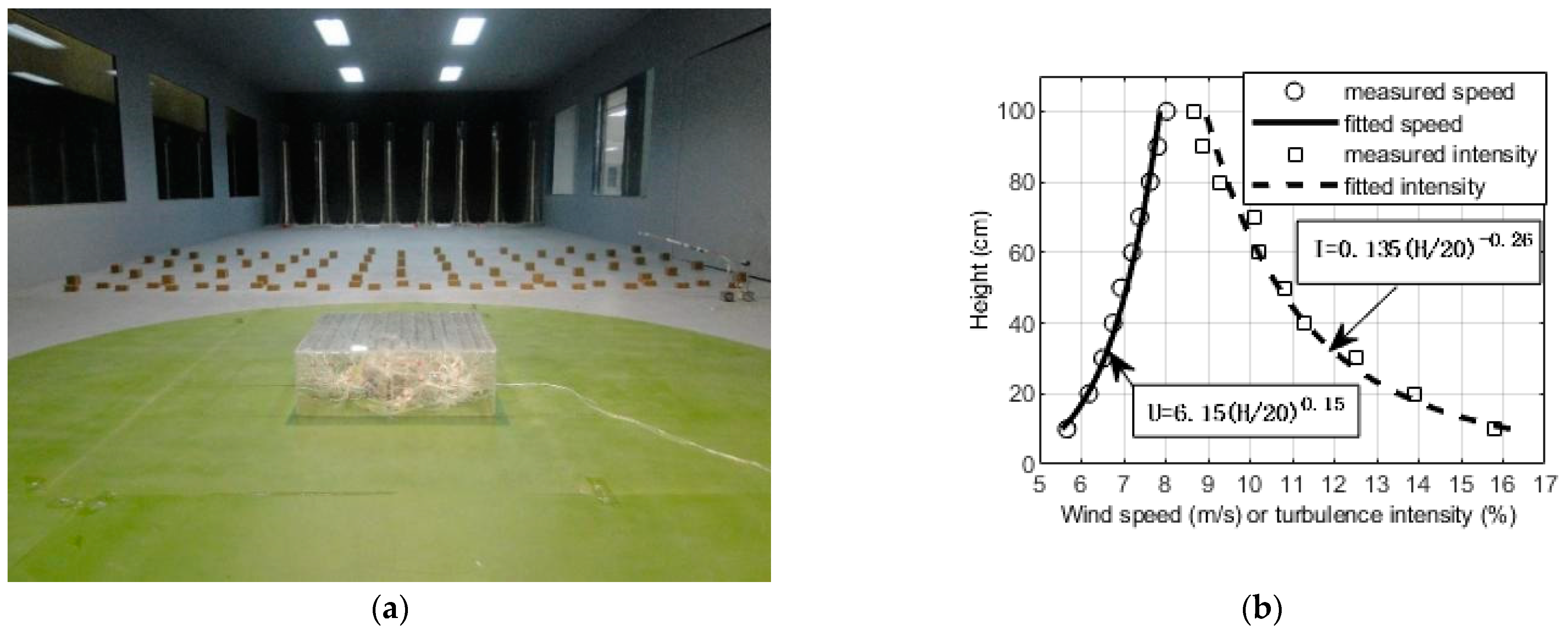
When the Gumbel distribution model and parameter estimation method are certain, the wind tunnel pressure test data of a low-rise building with a flat roof in Beijing Jiaotong University is used to analyze the influence of the time–distance and sample volume of maximum wind pressure samples on the uncertainty of extreme wind pressure predictions. Specifically, when the wind pressure test data are used to analyze the extreme wind pressure, the initial time histories of the wind pressure coefficient can be first normalized to obtain the time histories of the standard wind pressure coefficient:

$$Q\left(t\right)={\displaystyle \frac{Q^{\prime }(t)-\overline{Q^{\prime }}}{{\xi }_{Q^{\prime }}}}$$

(5)

where $Q^{\prime }\left(t\right)$ represents the initial time history of wind pressure coefficient; $\overline{Q^{\prime }}$ and ${\xi }_{Q^{\prime }}$ respectively represent the mean value and standard deviation of $Q^{\prime }\left(t\right)$; $Q\left(t\right)$ represents the normalized standard time history of the wind pressure coefficient. It should be noted here that the wind pressure coefficient samples are used for the prediction analysis of extreme wind pressure in this paper.

3. Extreme Value Analysis Based on Measured Wind Pressure Data

3.1. Wind Pressure Test

To analyze the influence of time–distance and sample volume changes on the prediction of extreme wind pressure, the uncertainty analysis of extreme wind pressure predictions is carried out based on the wind tunnel pressure test data of the low-rise building with a flat roof from Beijing Jiaotong University. Specifically, the test model of the low-rise building and the wind field layout are shown in Figure 1a. The test wind field in the process of the wind test is simulated with the class B terrain in the “Load Code for the Design of Building Structures” (GB50009-2012) [18] as a reference. The scale reduction ratio of the test model (600 mm × 600 mm × 200 mm) is 1/200, the average wind speed at the roof is 6.15 m/s, and the turbulence intensity is 13.5%. The average wind speed and turbulence intensity profiles [19] are shown in Figure 1b. The wind speed ratio is set to 1/6, and the time ratio is set to 3/100. The sampling frequency of the test is 312.5 Hz, and length of each sampling time is 18 s, which is equivalent to a 10 min sample collection duration for a full-scale structure. In this paper, the wind pressure time history samples obtained from 180 sampling times are selected for analysis, equivalent in number to the wind pressure time history samples with a sampling time of 30 h for a full-scale structure. A total of 210 measurement taps are set on the roof surface of the low-rise building test model, and the layout of the measurement taps is shown in Figure 2.

Figure 1. The test overview and the profiles of average wind speed and turbulence intensity. (a) Test model and wind field layout. (b) The profiles of average wind speed and turbulence intensity.

Figure 2. Arrangement of roof measurement taps (mm).

3.2. Setting of Time–Distance and Sample Volume

On the basis of the wind tunnel pressure test results of flat roof houses, multiple conditions of time–distance $t$ and sample volume $N$ are set to analyze the extreme wind pressure. Specifically, the working conditions are specified as follows: the time–distance $t$ is set at $t=2,5,10,20,30\min$, while the sample volume $N$ is designed as $N=5,10,15,20,30$. Therefore, a total of 25 condition combinations can be obtained for the time–distance and sample volume working conditions. For example, the working condition combination of $t=2$ and $N=10$ means that the total wind pressure time history samples are divided into a group of samples with a 2 min time–distance and continuously divided into 10 groups, and the 10 groups of samples, namely the sample time histories with 20 min time duration, are regarded as a subsection time history. For the subsection time history, the maximum wind pressure samples are extracted from the sample time histories of each $t=2$, and a group of maximum wind pressure samples with $N=10$ can be obtained. If the total sample time histories are divided into subsections, the maximum wind pressure samples of $N=10$ with $n$ groups can be obtained. Therefore, each group of maximum wind pressure samples is used to predict and analyze the extreme wind pressure. Furthermore, the specific combinations of all $\left(t,N\right)$ working conditions are shown in Table 1 below.

Table 1. The combinations of time–distance and sample volume condition.

		$\mathit{t}$(min)	2	5	10	20	30
	Duration (min) [Number of Sections] (Condition Serial Number)
$\mathit{N}$
5			10 [180] (1)	25 [72] (6)	50 [36] (11)	100 [18] (16)	150 [12] (21)
10			20 [90] (2)	50 [36] (7)	100 [18] (12)	200 [9] (17)	300 [6] (22)
15			30 [60] (3)	75 [24] (8)	150 [12] (13)	300 [6] (18)	450 [4] (23)
20			40 [45] (4)	100 [18] (9)	200 [9] (14)	400 [4] (19)	600 [3] (24)
30			60 [30] (5)	150 [12] (10)	300 [6] (15)	600 [3] (20)	900 [2] (25)

As shown in Table 1, different combinations of time–distance and sample volume correspond to different cases of sample division. For example, when the combination is $\left(t=2,N=5\right)$, the subsection wind pressure duration is 10 min, the total wind pressure time histories are divided into 180 subsections, and the condition $\left(t=2,N=5\right)$ is named as the sequence number 1.

3.3. Determination of the Parameter Estimation Method

According to the wind pressure test data, the wind pressure time history samples at three measurement taps on the flat roof are selected to calculate and analyze the parameter estimation methods, and the locations of three measurement taps ($\mathrm{Tap}1$, $\mathrm{Tap}2$, $\mathrm{Tap}3$) are shown in Figure 2. Taking a 10 min time interval as an example, the total wind pressure time history samples are divided into sections, and the corresponding maximum wind pressure sample is extracted, so that 180 maximum wind pressure samples can be obtained according to the total wind pressure time history samples at each measurement tap. Thus, the theoretical values of the $Y$ statistic corresponding to ME (Moment Estimation) method, MLE (Maximum Likelihood Estimation) method, BLUE (Best Linear Unbiased Estimation) method, and Gumbel method are calculated according to Equation (3), and the fitting comparison analysis is carried out with the empirical value of the $Y$ statistic. As shown in Figure 3, the comparison of $Y$ statistics fitting at three measurement taps under 60° wind direction is taken as an example for illustration. In addition, the normalized wind pressure coefficient extreme values are uniformly called extreme wind pressure.

Figure 3. The comparison of $Y$ statistics corresponding to different parameter estimation methods.

In Figure 3, the $Y$ statistics corresponding to different parameter estimation methods have significant differences in the fitting comparison effects. To select a better parameter estimation method, according to the fitting comparison effect of $Y$ statistics corresponding to different parameter estimation methods, the determination coefficient $R^2$ is further used for the goodness-of-fit test. In particular, the $R^2$ value is calculated using Equation (6). The calculation results of $R^2$ corresponding to different parameter estimation methods are shown in Table 2.

$$R^2=1-{\displaystyle \frac{{\displaystyle \sum _{i=1}^n{\left[{q^{\prime }}_i-{\overleftarrow{F}}_1\left(p_i\right)\right]}^2}}{{\displaystyle \sum _{i=1}^n{\left({q^{\prime }}_i-{\overline{q}}^{\prime }\right)}^2}}}$$

(6)

where $R^2$ represents the determination coefficient; $n$ represents the number of the total maximum wind pressure samples; $p_i$ represents the empirical probability of the $i$th maximum wind pressure order statistic ${q^{\prime }}_i$, and $p_i$ can be calculated with Equation (4). ${\overleftarrow{F}}_1\left(•\right)$ is the inverse function of the Gumbel distribution function. ${\overline{q}}^{\prime }$ represents the average of the maximum wind pressure order statistic. According to the definition of the $R^2$, when the $R^2$ value corresponding to the parameter estimation method is closer to 1, the goodness of fit of the method is higher.

Table 2. The $R^2$ values corresponding to different parameter estimation methods.

Methods	${\mathit{R}}^2$
	$\mathbf{T}\mathbf{a}\mathbf{p}1$	$\mathbf{T}\mathbf{a}\mathbf{p}2$	$\mathbf{T}\mathbf{a}\mathbf{p}3$
ME	0.99	0.99	0.99
MLE	0.99	0.99	0.99
BLUE	0.96	0.95	0.96
Gumbel	0.99	0.99	0.99

It can be seen from Figure 3 and Table 2 that the determination coefficient $R^2$ values corresponding to the ME (Moment Estimation) method, MLE (Maximum Likelihood Estimation) method, and Gumbel estimation method are similar and close to 1, indicating that the $Y$ statistics corresponding to the three methods have better fitting effects. Therefore, the MLE method may be used to estimate the distribution parameters of the Gumbel distribution model.

4. Result Analysis

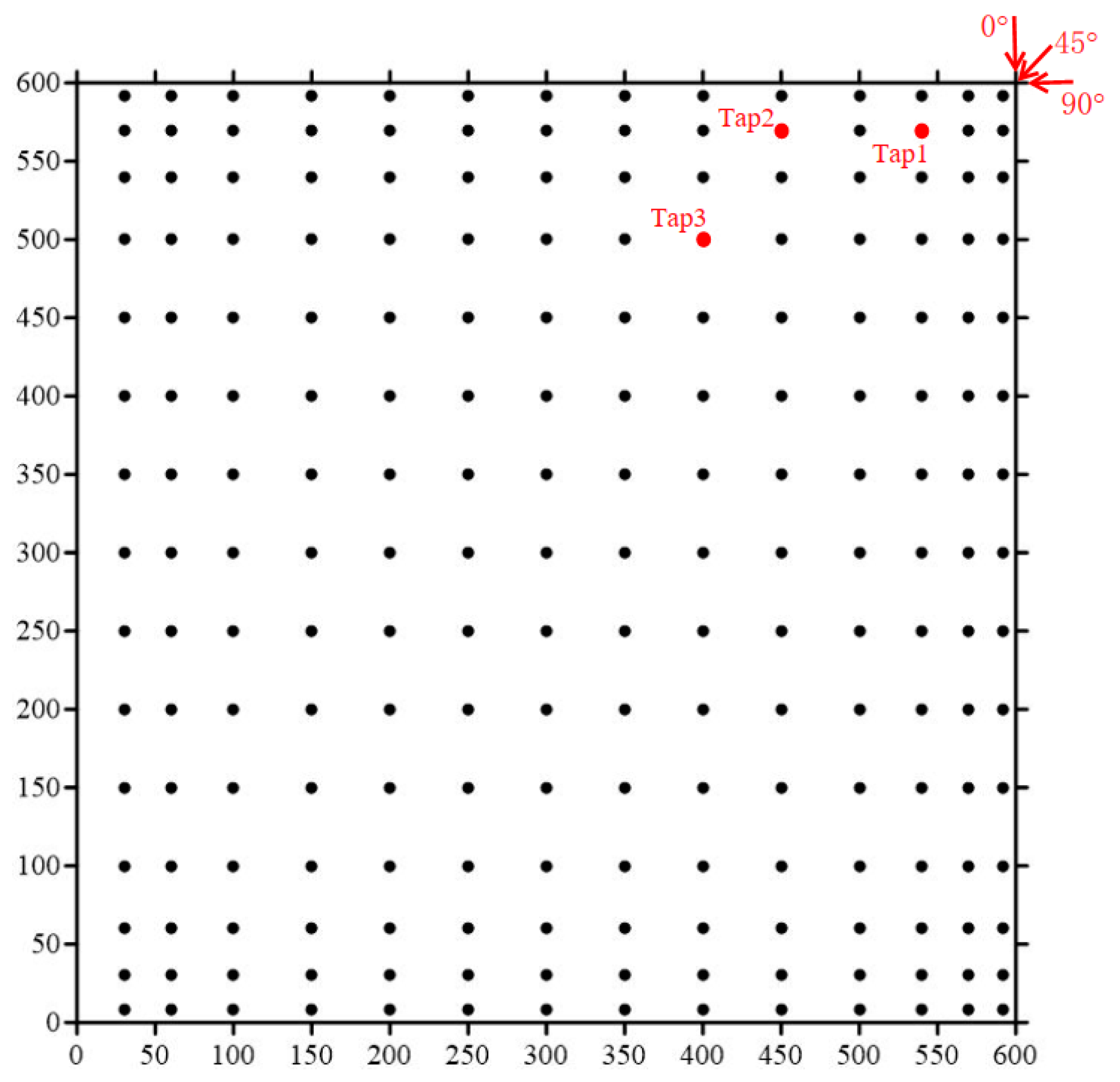
According to the above, the influence of time–distance $t$ and sample volume $N$ on the uncertainty of extreme wind pressure prediction is further analyzed. Firstly, the prediction values of theoretical extreme wind pressure $q_{\mathrm{gum}}$ corresponding to all combinations of $t$ and $N$ working conditions are calculated based on the wind pressure time history samples at three measurement taps under 0°, 45°, 60°, and 90° wind directions. At the same time, the empirical extreme value $q_{\mathrm{emp}}$ and 99% confidence interval (${\overline{q}}_{\mathrm{emp}}$ is the mean, $q_{\mathrm{emp},\mathrm{up}}$ is the upper limit, and $q_{\mathrm{emp},\mathrm{dn}}$ is the lower limit) of $q_{\mathrm{emp}}$ are calculated for each time–distance condition. The $q_{\mathrm{gum}}$ values and $q_{\mathrm{emp}}$ values with an 80% guarantee rate [13] are taken as an example for illustration. The analysis results are shown in Figure 4. In addition, the “shape symbols” corresponding to different $N$ conditions indicate the corresponding extreme values $q_{\mathrm{gum}}$ in Figure 4.

Figure 4. The comparison between the $q_{\mathrm{gum}}$ and $q_{\mathrm{emp}}$ corresponding to all $\left(t,N\right)$ conditions.

Figure 4 shows that the mean value ${\overline{q}}_{\mathrm{emp}}$ of the empirical extreme value $q_{\mathrm{emp}}$ increases with the increase of time–distance $t$ for one thing, and the width of the 99% confidence interval of $q_{\mathrm{emp}}$ tends to decrease when $t$ is shorter than 30 min for another. When $t=30\min$, only a set of maximum wind pressure samples can be obtained, and in the calculation of the confidence interval for $q_{\mathrm{emp}}$, only the unique estimation value of $q_{\mathrm{emp}}$ with the 80% guarantee rate can be determined. Here, in the determination of the variation interval of $q_{\mathrm{emp}}$ corresponding to the working condition of $t=30\min$, the minimum value of the total maximum wind pressure sample is taken as the lower limit of the interval, and the maximum value is taken as the upper limit of the interval. Therefore, the width of the interval corresponding to the $t=30\min$ condition is large. When $t$ is shorter than 10 min, the mean value ${\overline{q}}_{\mathrm{gum}}$ of the theoretical extreme wind pressure $q_{\mathrm{gum}}$ shows an increasing trend with the increase of sample volume $N$, but when $t$ is greater than 10 min, the change rule of ${\overline{q}}_{\mathrm{gum}}$ with $N$ is not obvious. Under a certain $N$ condition, the ${\overline{q}}_{\mathrm{gum}}$ value shows an obvious increasing trend with the increase of $t$, and when $t$ is greater than 10 min, the change of ${\overline{q}}_{\mathrm{gum}}$ tends to be steady.

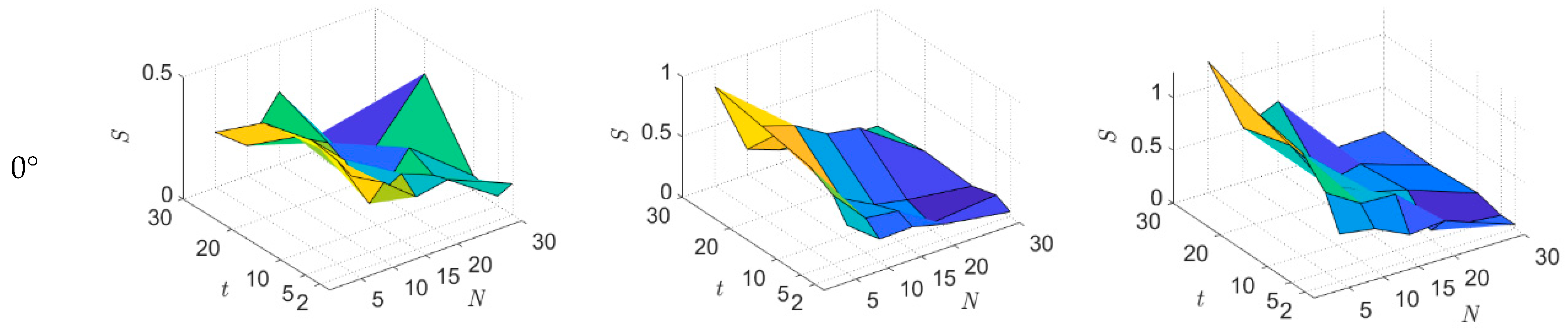
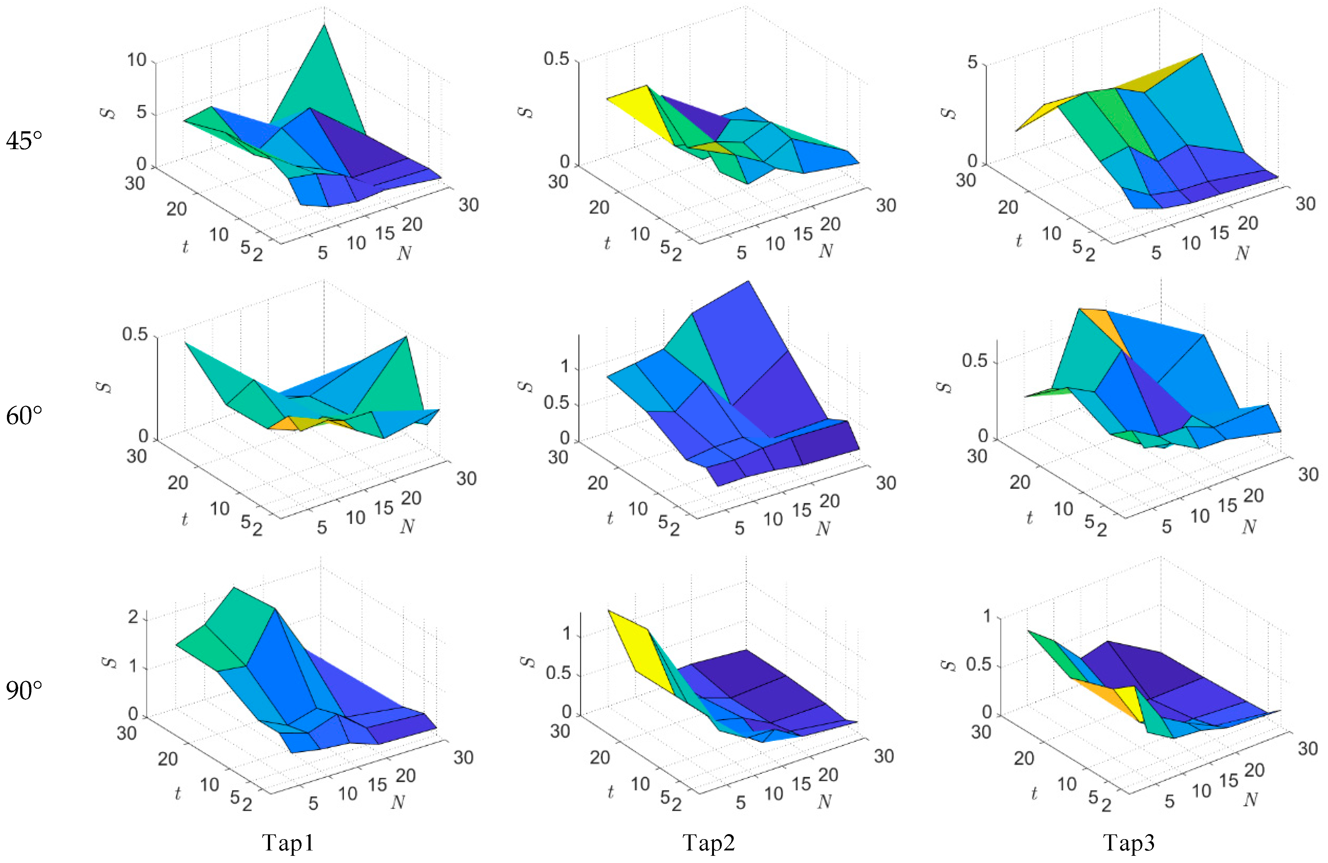
According to the above analysis results, the prediction accuracy of the theoretical extreme wind pressure $q_{\mathrm{gum}}$ corresponding to different condition combinations of time–distance $t$ and sample volume $N$ is further analyzed, and the mean square error values between the theoretical extreme wind pressure $q_{\mathrm{gum},i}$ value corresponding to each subsection and the mean ${\overline{q}}_{\mathrm{emp}}$ of the empirical extreme wind pressure $q_{\mathrm{emp}}$ are further calculated according to Equation (7). The calculation results are shown in Figure 5. Meanwhile, the corresponding guarantee rates of $q_{\mathrm{gum},i}$ and $q_{\mathrm{emp}}$ are both 80%, and the mean square error is calculated as follows:

$$S={\displaystyle \frac{1}{n}}{\displaystyle \sum _i^n{\left(q_{\mathrm{gum},i}-{\overline{q}}_{\mathrm{emp}}\right)}^2} ,$$

(7)

where $S$ represents the mean square error value; $n$ represents the corresponding number of subsections under a certain working condition $\left(t,N\right)$; $q_{\mathrm{gum},i}$ represents the theoretical extreme wind pressure corresponding to the time history of the $i$th subsection.

Figure 5. The $S$ values between ${\overline{q}}_{\mathrm{emp}}$ and $q_{\mathrm{gum}}$ corresponding to all $\left(t,N\right)$ conditions.

Figure 5 shows that the $S$ values decrease with the increase of $N$ condition under different $t$ conditions. However, under the condition of a certain $N$, the $S$ value has no obvious regular patterns of change with the change of $t$; when $N$ is small and $t$ is greater than 10 min, the corresponding $S$ value is larger. It can be concluded that the increase in $N$ can improve the prediction accuracy of extreme wind pressure $q_{\mathrm{gum}}$ under a certain $t$.

The above analysis takes the mean value ${\overline{q}}_{\mathrm{emp}}$ of the empirical wind pressure extreme value $q_{\mathrm{emp}}$ as the reference value and quantifies the prediction accuracy of $q_{\mathrm{gum}}$ by calculating the mean square error $S$ between the ${\overline{q}}_{\mathrm{emp}}$ value and the theoretical extreme wind pressure $q_{\mathrm{gum},i}$ value of each subsection. However, it should be noted that the above analysis process is only based on the existing wind pressure time histories with the fixed total time and cannot be compared and analyzed with the $q_{\mathrm{gum}}$ prediction results corresponding to the wind pressure time histories of other total times. Therefore, the corresponding $q_{\mathrm{gum}}$ prediction results under different $\left(t,N\right)$ conditions can be converted into a unified reference frame for comparison. At the same time, according to the analysis results in Figure 4, the change in time–distance $t$ has a greater impact than the change in sample volume $N$ on the $q_{\mathrm{gum}}$ prediction value, and the change rule is obvious. Therefore, without loss of generality, assuming that a certain time–distance $T$ is the standard time–distance, the $q_{\mathrm{gum}}$ prediction values corresponding to different $t$ working conditions are uniformly converted into the corresponding wind pressure conversion extreme value $q_{\mathrm{gumtr}}$ under the standard time–distance $T$, and the accuracy of $q_{\mathrm{gumtr}}$ is consistent with the accuracy of $q_{\mathrm{gum}}$. Therefore, in this paper, it may be assumed that the time–distance $T=60\min$ is used as the standard time–distance, and the $q_{\mathrm{gum}}$ prediction values corresponding to different $t$ working conditions are converted into $q_{\mathrm{gumtr}}$ corresponding to the standard $T=60\min$ working conditions. At the same time, in order to compare and illustrate the prediction accuracy of $q_{\mathrm{gumtr}}$, the corresponding $q_{\mathrm{gum}}$ prediction value and $q_{\mathrm{emp}}$ value and its mean value ${\overline{q}}_{\mathrm{emp}}$ under the $t=T=60\min$ working condition are taken as the standard theoretical extreme wind pressure ${q^{*}}_{\mathrm{gum}}$ and the standard empirical extreme wind pressure ${q^{*}}_{\mathrm{emp}}$ and its mean value ${{\overline{q}}^{*}}_{\mathrm{emp}}$, respectively. Therefore, the prediction accuracy of $q_{\mathrm{gumtr}}$ corresponding to different condition $\left(t,N\right)$ combinations can be compared and analyzed. It should be noted that the calculation of $q_{\mathrm{gumtr}}$ ignores the errors in the transformation process.

According to the above analysis, we can realize the calculation of the wind pressure conversion extreme value $q_{\mathrm{gumtr}}$ by the conversion between Gumbel distribution parameters under different time–distance $t$ conditions; the conversion formula between distribution parameters is as follows:

$$\left\{\begin{array}{l}{\sigma }_T={\sigma }_t\\ {\mu }_T={\mu }_t+{\sigma }_t\cdot \ln (T/t)\end{array}\right.,t<T,$$

(8)

where ${\sigma }_T$ and ${\mu }_T$ represent, respectively, the scale parameter and location parameter of the Gumbel distribution model corresponding to a standard time–distance $T$; ${\sigma }_t$ and ${\mu }_t$ denote, respectively, the scale parameter and location parameter corresponding to the small time–distance $t$. Therefore, according to the transformed Gumbel distribution parameters, the corresponding wind pressure conversion extreme value $q_{\mathrm{gumtr}}$ can be calculated and determined.

To compare and analyze the accuracy of $q_{\mathrm{gumtr}}$ corresponding to different working conditions of time–distance $t$ and sample volume $N$, the ratio of the corresponding $q_{\mathrm{gumtr}}$ values under various working conditions to the standard theoretical extreme wind pressure ${q^{*}}_{\mathrm{gum}}$ is calculated as follows:

$${\delta }^{\prime }={\displaystyle \frac{q_{\mathrm{gumtr}}}{{q^{*}}_{\mathrm{gum}}}},$$

(9)

where ${\delta }^{\prime }$ represents the wind pressure conversion ratio of $q_{\mathrm{gumtr}}$ to ${q^{*}}_{\mathrm{gum}}$; when the ${\delta }^{\prime }$ value is closer to 1, it indicates that the prediction accuracy of the extreme wind pressure conversion value $q_{\mathrm{gumtr}}$ is higher, which further indicates that the prediction accuracy of the original theoretical extreme wind pressure $q_{\mathrm{gum}}$ is higher.

To further compare and analyze the influence of different working conditions $\left(t,N\right)$ on the extreme wind pressure predictions, the prediction values of $q_{\mathrm{gum}}$ with the 80% guarantee rate corresponding to different time–distance $t$ are converted into the $q_{\mathrm{gumtr}}$ corresponding to standard time–distance $T$, and the wind pressure conversion ratio ${\delta }^{\prime }$ value corresponding to each subsection is calculated according to Equation (9), the mean value $\overline{{\delta }^{\prime }}$, and the confidence interval with a certain confidence degree. Here, the 95% confidence interval of ${\delta }^{\prime }$ is taken as an example to illustrate its range of variation, where ${{\delta }^{\prime }}_{\mathrm{dn}}$ is the lower limit and ${{\delta }^{\prime }}_{\mathrm{up}}$ is the upper limit of the interval. Based on the measured wind pressure data at all measurement taps on the flat roof under four wind directions (0°, 45°, 60°, and 90°), the mean value $\overline{{\delta }^{\prime }}$ corresponding to all $\left(t,N\right)$ combinations (see Table 1) and the 95% confidence interval is calculated and determined at all measurement taps respectively, and the change of the $\overline{{\delta }^{\prime }}$ value with the standard theoretical extreme wind pressure ${q^{*}}_{\mathrm{gum}}$ 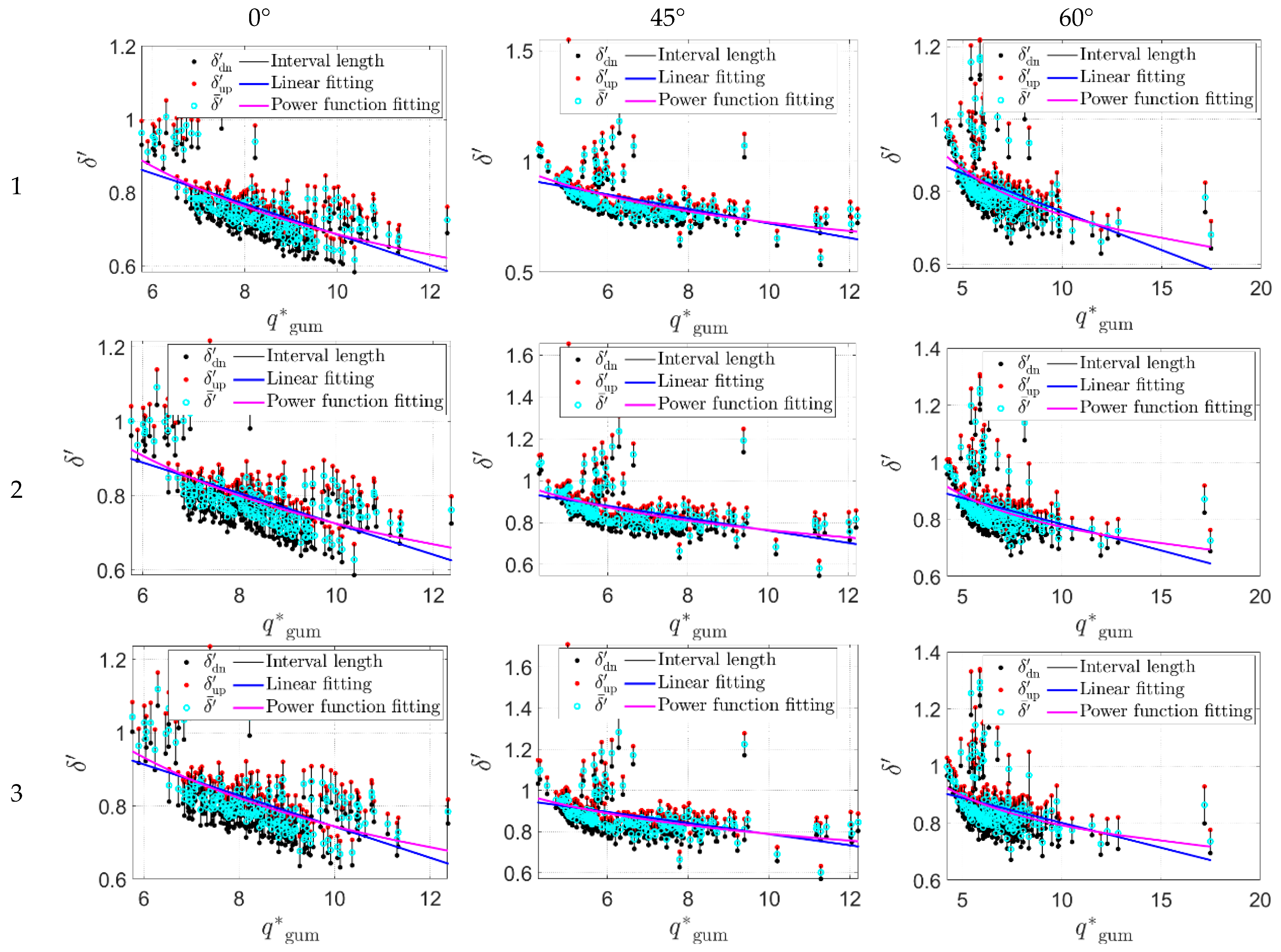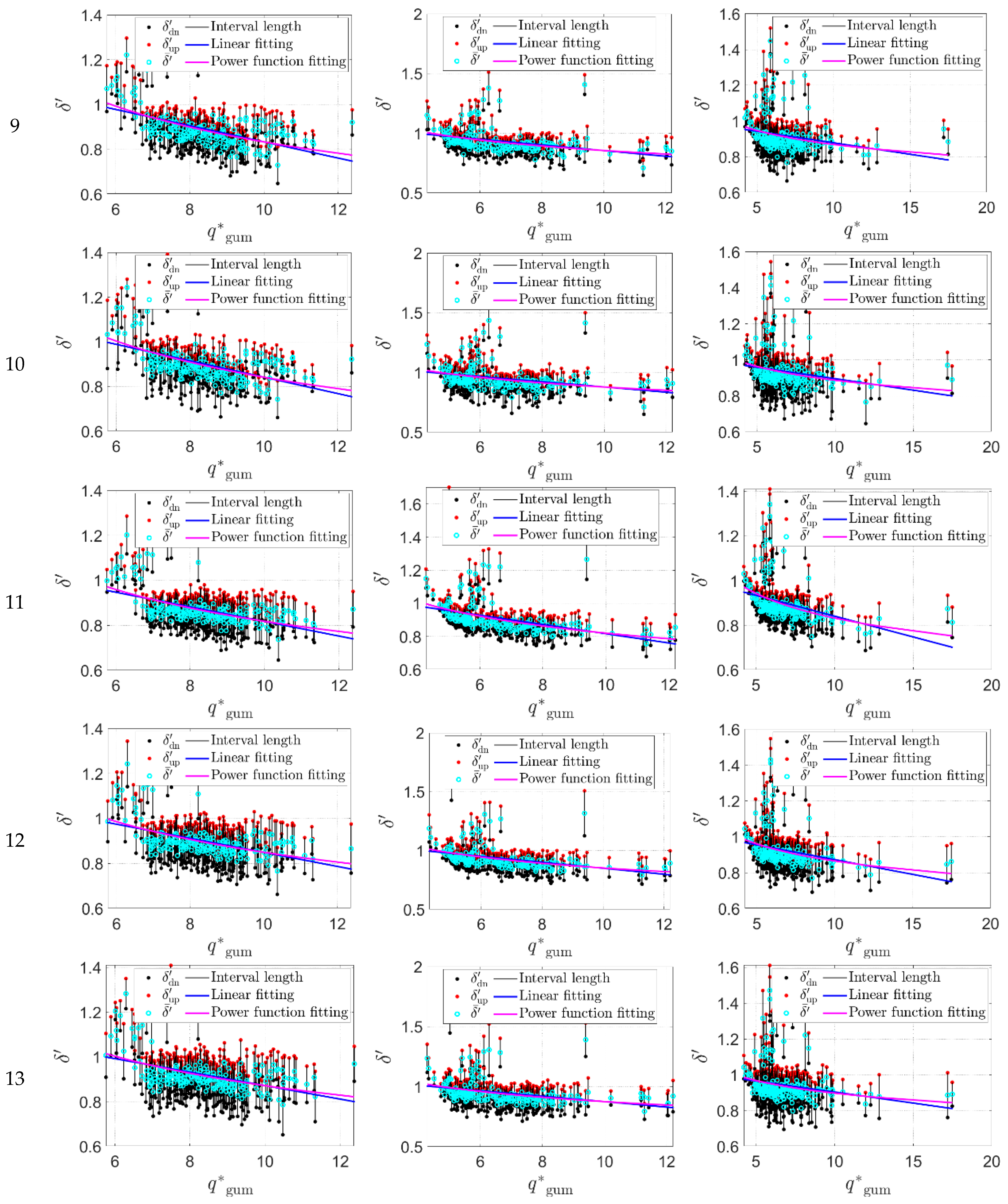is further fitted and analyzed with the use of the linear relationship and the power function relationship. Specifically, the ${\delta }^{\prime }$ calculation results corresponding to ${q^{*}}_{\mathrm{gum}}$ with the 80% guarantee rate in 0°, 45°, and 60° wind directions are illustrated as examples in Figure 6. As shown in Figure 6, the results corresponding to the first 15 working conditions are presented due to consideration of the length of the article, and the serial number of the working condition is 1~15.

Figure 6. The mean $\overline{{\delta }^{\prime }}$ and 95% confidence interval results of ${\delta }^{\prime }$ values corresponding to different working conditions $\left(t,N\right)$ at all measurement taps.

It can be seen from Figure 6 that under the action of different wind directions, for a certain working condition, the mean value $\overline{{\delta }^{\prime }}$ of the wind pressure conversion ratio ${\delta }^{\prime }$ decreases first and then becomes gentle with the increase of the standard theoretical extreme value ${q^{*}}_{\mathrm{gum}}$. Compared with the linear fitting curve, the power function fitting curve is closer to the change trend of $\overline{{\delta }^{\prime }}$. For different working conditions $\left(t,N\right)$, when time–distance $t$ is fixed, for example, when conditions are 1~5, 6~10, or 11~15, with the increase of sample volume $N$, the decrease of $\overline{{\delta }^{\prime }}$ with the increase of ${q^{*}}_{\mathrm{gum}}$ tends to be smooth, and the number of measurement taps whose $\overline{{\delta }^{\prime }}$ value is greater than 0.8 increases and $\overline{{\delta }^{\prime }}$ values approach 1. 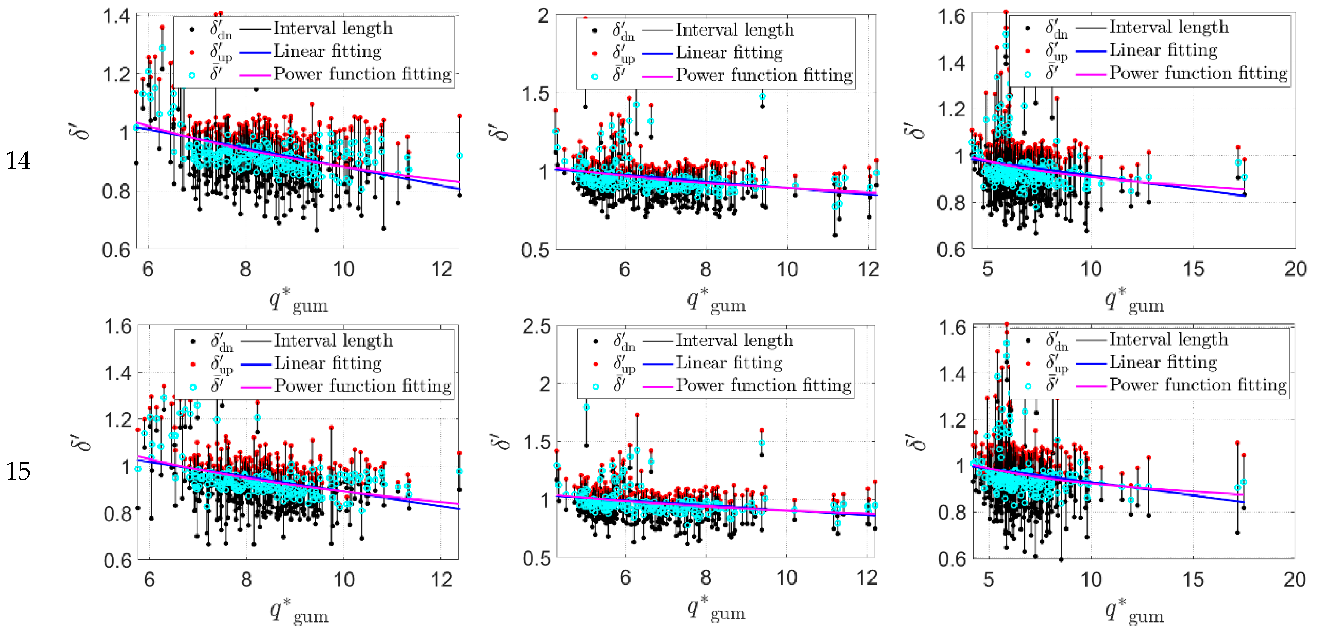When $N$ is certain (such as conditions with serial numbers 1, 6, 11, conditions with serial numbers 2, 7, 12, conditions with serial numbers 3, 8, 13, conditions serial numbers 4, 9, 14, or conditions serial numbers 5, 10, 15), with the increase of $t$, the decrease of the $\overline{{\delta }^{\prime }}$ with the increase of the ${q^{*}}_{\mathrm{gum}}$ obviously tends to be gentle, and the larger the $t$ value is, the closer to 1 the $\overline{{\delta }^{\prime }}$ value is.

5. Empirical Fitting Relationship of Wind Pressure Conversion Ratio

According to the analysis in Figure 6, the wind pressure conversion ratio ${\delta }^{\prime }$ approximately follows a power function change relationship with the change of the standard theoretical extreme wind pressure ${q^{*}}_{\mathrm{gum}}$, so the empirical correspondence between the ${\delta }^{\prime }$ and ${q^{*}}_{\mathrm{gum}}$ is further established as follows:

$${\delta }^{\prime }=a\cdot {{q^{*}}_{\mathrm{gum}}}^b,$$

(10)

where $a$ and $b$ are the distribution parameters of the power function relationship.

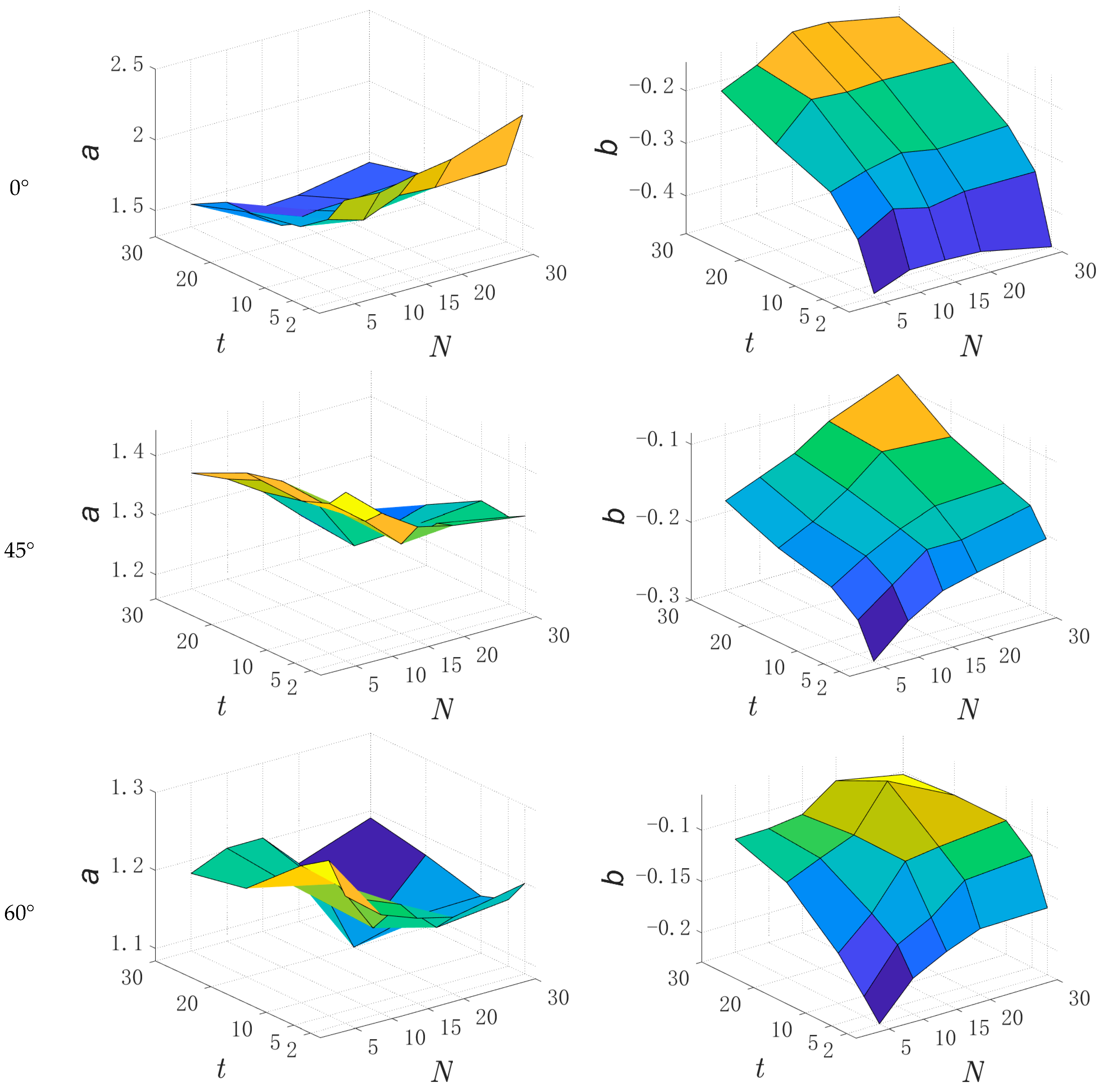
According to the empirical formula established above, the power function distribution parameter $a$ and $b$ values of the corresponding ${\delta }^{\prime }$ under different working conditions of time–distance $t$ and sample volume $N$ are calculated and determined. Thus, the empirical relation expressions of parameters $a$ and $b$ concerning $t$ and $N$ are further fitted. 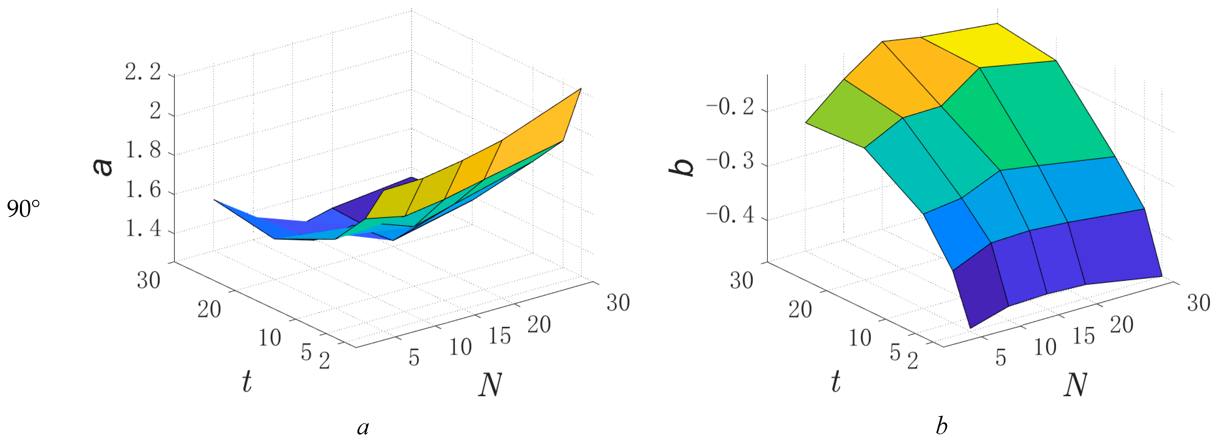Specifically, the corresponding parameter $a$ and $b$ values under different wind directions and different conditions $\left(t,N\right)$ are statistically analyzed, and the results are shown in Figure 7.

Figure 7. The parameter $a$ and $b$ values under different conditions $\left(t,N\right)$.

In Figure 7, under the action of 0° and 90° wind directions, the parameter $a$ shows a power function relationship with the increase of time–distance $t$. Meanwhile, with the change of the sample volume $N$, the change pattern of $a$ is not obvious. However, when the $t$ is large, the change trend of $a$ with $N$ is a slight power function. The parameter $b$ obviously shows a logarithmic relationship with the increase of $t$ and remains basically stable with the change of $N$. Under the action of 45° and 60° wind directions, the parameter $a$ changes with $N$ approximately in a power function relationship, but the change pattern of the parameter $a$ with $t$ is relatively unobvious, and when $N$ is large, the change trend of $a$ with $t$ is a slight power function. The parameter $b$ changes logarithmically with the increase of $t$ and $N$, and the change rule is obvious. In addition, since the parameters $a$ and $b$ have certain volatility with the change of $t$ and $N$, sine or cosine functions can be used to coordinate the change rule. Further, according to the preliminary analysis and judgment of the change rules of parameters $a$ and $b$ with $t$ and $N$, the empirical relations of the parameters $a$ and $b$ with $t$ and $N$ are approximately constructed as follows.

For 0° and 90° wind directions:

$$a=k_{a,1}\cdot t^{k_{a,2}}+k_{a,3}\cdot N^{k_{a,4}}+k_{a,5}\cdot \sin (N)+k_{a,6}\cdot \cos (N)+k_{a,7},$$

(11)

$$b=k_{b,1}\cdot \ln \left(k_{b,2}\cdot t\right)+k_{b,3}\cdot \sin (N)+k_{b,4}\cdot \cos (N)+k_{b,5}.$$

(12)

For 45° and 60° wind directions:

$$a=k_{a,1}\cdot N^{k_{a,2}}+{k^{\prime }}_{a,3}\cdot t^{k_{a,4}}+{k^{\prime }}_{a,5}\cdot \sin (t)+k_{a,6}\cdot \cos (t)+k_{a,7},$$

(13)

$$b=k_{b,1}\cdot \ln \left(k_{b,2}\cdot N\right)+2k_{b,3}\cdot \ln \left(k_{b,4}\cdot t\right)+k_{b,5},$$

(14)

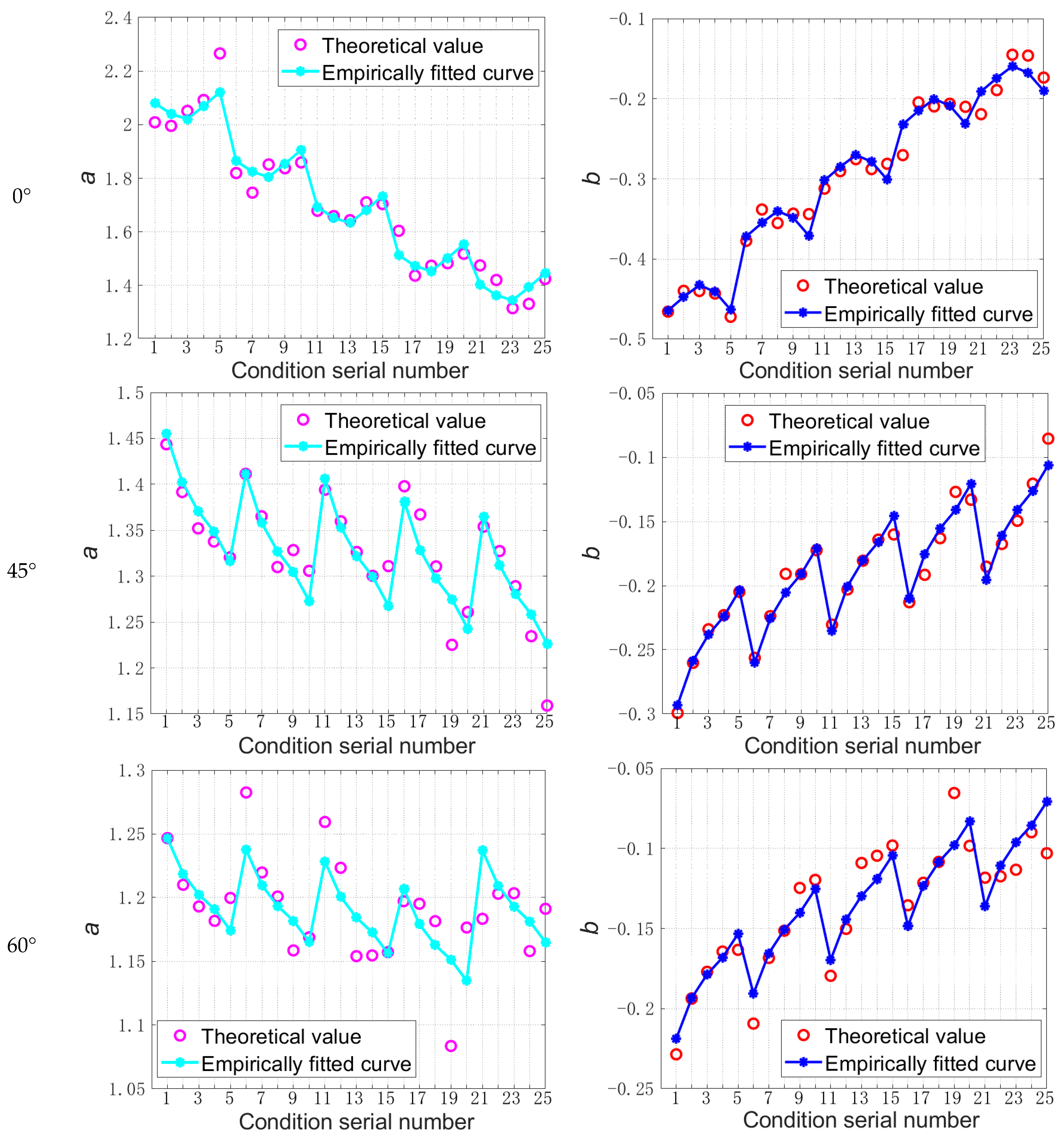
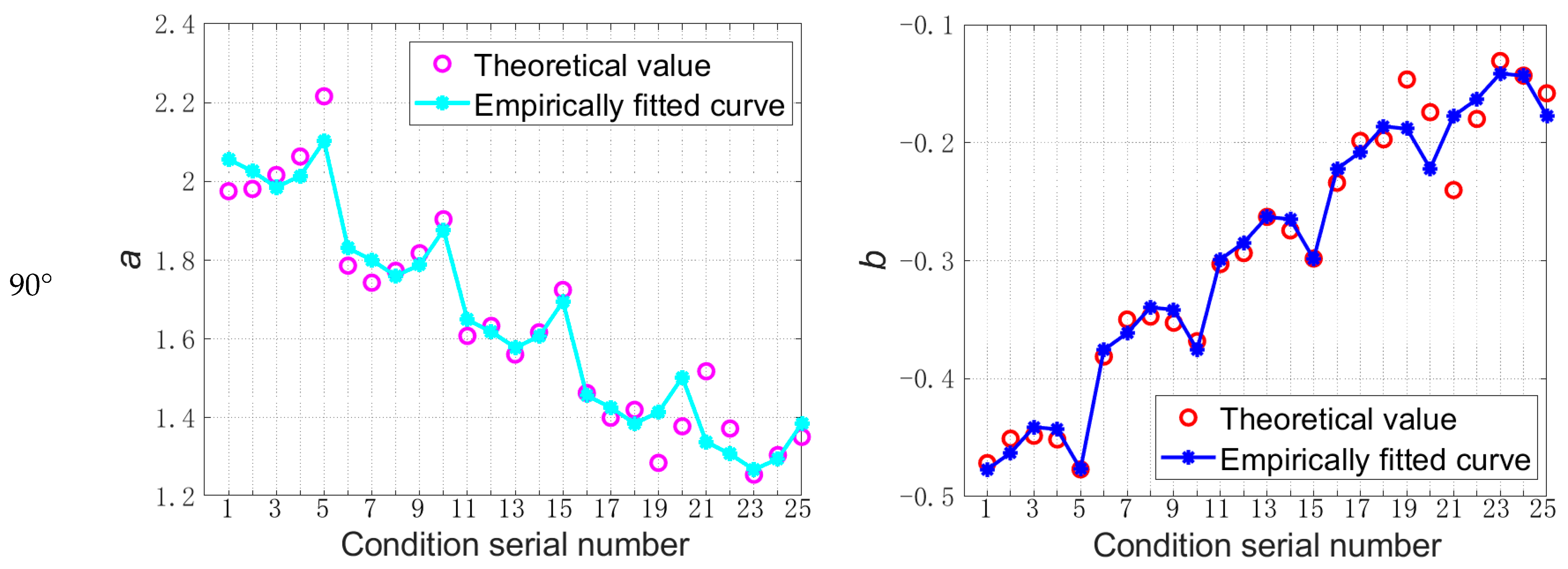
where $k_{a,j}$ denotes the $j$th fitting parameter in the empirical formula of the parameter $a$ concerning $t$ and $N$. $k_{b,j}$ denotes the $j$th fitting parameter in the empirical formula of the parameter $b$ with respect to $t$ and $N$. Therefore, the least square fitting method is used to further determine the fitting parameter values in the empirical formula. Specifically, the fitting comparison results of the empirical formula corresponding to the 1~25 working conditions are shown in Figure 8, and the corresponding fitting parameter values are shown in Table 3.

Figure 8. The comparison fitting of empirical and theoretical values of parameter $a$ and $b$ values under different working conditions.

Table 3. The fitted values of parameters $a$ and $b$ under different wind angles.

Wind	Parameters	Empirically Fitted Parameters
0°	$a$	$k_{a,1}$	$k_{a,2}$	$k_{a,3}$	$k_{a,4}$	$k_{a,5}$	$k_{a,6}$	$k_{a,7}$
		−3.423	0.064	5.767	0.004	−0.027	0.042	−0.188
	$b$	$k_{b,1}$	$k_{b,2}$	$k_{b,3}$	$k_{b,4}$	$k_{b,5}$
		0.101	3.145	0.013	−0.010	−0.634
45°	$a$	$k_{a,1}$	$k_{a,2}$	$k_{a,3}$	$k_{a,4}$	$k_{a,5}$	$k_{a,6}$	$k_{a,7}$
		−2.452	0.029	0.407	−0.080	0.005	−0.011	3.631
	$b$	$k_{b,1}$	$k_{b,2}$	$k_{b,3}$	$k_{b,4}$	$k_{b,5}$
		0.050	2.885	0.018	5.698	−0.514
60°	$a$	$k_{a,1}$	$k_{a,2}$	$k_{a,3}$	$k_{a,4}$	$k_{a,5}$	$k_{a,6}$	$k_{a,7}$
		−6.013	0.007	0.904	−4.467	−0.016	0.002	7.298
	$b$	$k_{b,1}$	$k_{b,2}$	$k_{b,3}$	$k_{b,4}$	$k_{b,5}$
		0.037	3.088	0.015	4.297	−0.384
90°	$a$	$k_{a,1}$	$k_{a,2}$	$k_{a,3}$	$k_{a,4}$	$k_{a,5}$	$k_{a,6}$	$k_{a,7}$
		−2.778	0.081	4.205	0.006	−0.045	0.027	0.696
	$b$	$k_{b,1}$	$k_{b,2}$	$k_{b,3}$	$k_{b,4}$	$k_{b,5}$
		0.111	2.017	0.019	−0.006	−0.612

As shown in Figure 8, the deviations between the empirical values and theoretical values of parameters $a$ and $b$ corresponding to different conditions of time–distance and sample volume are small under different wind directions, and the fitting change trend of the empirical and theoretical values is basically consistent. To further illustrate the relative deviation between empirical and theoretical values, based on the analytical results in Figure 8, the average relative errors between the empirical and theoretical parameter values are further calculated [20,21], and the calculation formula is given in Equation (15). The corresponding calculation results are shown in Table 4.

$$\eta ={\displaystyle \frac{1}{m}}{\displaystyle \sum _{j=1}^m\left(\frac{C_{\mathrm{emp}, j}-C_{\mathrm{the}, j}}{C_{\mathrm{the}, j}}\right)},$$

(15)

where $\eta$ represents the average relative error; $m$ represents the number of parameters and is also the number of $\left(t,N\right)$ working conditions; $C_{\mathrm{emp}, j}$ represents the $j$th empirical parameter value; $C_{\mathrm{the}, j}$ represents the $j$th theoretical parameter value.

Table 4. The average relative error between empirical and theoretical values of the parameters.

Wind Direction	${\mathit{\eta }}_{\mathit{a}}$	${\mathit{\eta }}_{\mathit{b}}$
0°	0.025	0.053
45°	0.014	0.043
60°	0.018	0.096
90°	0.031	0.062

Note: ${\eta }_a$ represents the average relative error corresponding to parameter $a$; ${\eta }_b$ represents the average relative error corresponding to parameter $b$.

According to Table 4, the $\eta$ values between the empirical and theoretical values of the parameters $a$ and $b$ are basically kept within 5% under different wind directions, and the maximum is no more than 10%. Therefore, the calculation accuracy of the empirical formula is kept within the applicable range, and the empirical formula has better applicability.

6. Discussion

Based on the above analysis, under the condition of a given volume of samples, the prediction value of extreme wind pressure increases first and then remains stable with the increase of time–distance. However, under the condition of a given time–distance, the influence of the change of sample volume on the prediction value of extreme wind pressure is not obvious. Specifically, when the time–distance is less than 20 min, the extreme wind pressure slightly increases with the increase of sample volume, but the change law is not obvious. When the time–distance is greater than or equal to 20 min, the influence of the variation of sample volume on the prediction values of extreme wind pressure has no obvious change law. In addition, for the different conditions of time–distance and sample volume, the mean square error values between the theoretical extreme wind pressure and the empirical extreme wind pressure have no obvious change law with the increase of time–distance, but are obviously affected by the change of sample volume. For the conversion value of extreme wind pressure, the corresponding conversion values are closer to the standard extreme wind pressure values when the time–distance and sample volume are large, which indicates that the larger time–distance and sample volume can effectively improve the prediction accuracy of the extreme wind pressure.

7. Conclusions and Recommendations

In summary, a larger time–distance and sample volume can effectively reduce the bias and uncertainty of extreme wind pressure. Meanwhile, the empirical value of the wind pressure conversion ratio calculated by the established empirical formula has a smaller deviation with theoretical value, and the maximum deviation does not exceed 10%. Therefore, the empirical calculation formula of the wind pressure conversion ratio can provide a certain calculation method for the analysis of the prediction accuracy of the extreme wind pressure.

It is worth noting that the test models and analysis conditions selected in this paper are limited, and it is necessary to further use the wind pressure data of different test models to predict and analyze the extreme wind pressure, so as to provide a reference and basis for the reasonable value of time–distance and sample volume. In addition, the applicability of the proposed empirical formula for the wind pressure conversion ratio needs to be further verified.

References

1. Sadek, F.; Simiu, E. Peak non-Gaussian wind effects for database-assisted low-rise building design. J. Eng. Mech. 2002, 128, 530–539. [Google Scholar] [CrossRef]
2. Holmes, J.D.; Cochran, L.S. Probability distributions of extreme pressure coefficients. J. Wind Eng. Ind. Aerodyn. 2003, 91, 893–901. [Google Scholar] [CrossRef]
3. Kasperski, M. Specification of the design wind load based on wind tunnel experiments. J. Wind Eng. Ind. Aerodyn. 2003, 91, 527–541. [Google Scholar] [CrossRef]
4. Harris, R.I. A new direct version of the Cook-Mayne method for wind pressure probabilities in temperate storms. J. Wind Eng. Ind. Aerodyn. 2005, 93, 581–600. [Google Scholar] [CrossRef]
5. Kasperski, M. Design wind loads for a low-rise building taking into account directional effects. J. Wind Eng. Ind. Aerodyn. 2007, 95, 1125–1144. [Google Scholar] [CrossRef]
6. Huang, G.; Luo, Y.; Gurley, K.R.; Ding, J. Revisiting moment-based characterization for wind pressures. J. Wind Eng. Ind. Aerodyn. 2016, 151, 158–168. [Google Scholar] [CrossRef]
7. Luo, Y.; Huang, G. Characterizing dependence of extreme wind pressures. J. Struct. Eng. 2017, 143, 04016208. [Google Scholar] [CrossRef]
8. Davenport, A.G. Note on the distribution of the largest value of a random function with application to gust loading. Proc. Inst. Civ. Eng. 1964, 28, 187–196. [Google Scholar] [CrossRef]
9. Wang, F.; Quan, Y.; Gu, M. An extreme-value estimation method of non-Gaussian wind pressure based on generalized extreme value theory. Mech. Eng. 2013, 30, 44–49. [Google Scholar]
10. Ding, J.; Chen, X. Assessment of methods for extreme value analysis of non-Gaussian wind effects with short-term time history samples. Eng. Struct. 2014, 80, 75–88. [Google Scholar] [CrossRef]
11. Huang, P.; Lan, X.; Zhong, Q. Extreme value estimation method for measured wind pressures on low-rise buildings based on the peaks over threshold model. J. Vib. Shock. 2019, 38, 33–40. [Google Scholar]
12. Hong, H.P.; Ye, W.; Li, S.H. Sample size effect on the reliability and calibration of design wind load. Struct. Infrastruct. Eng. 2016, 12, 752–764. [Google Scholar] [CrossRef]
13. Gavanski, E.; Gurley, K.R.; Kopp, G.A. Uncertainties in the estimation of local peak pressures on low-rise buildings by using the Gumbel distribution fitting approach. J. Struct. Eng. 2016, 142, 04016106. [Google Scholar] [CrossRef]
14. Li, S.H.; Kilpatrick, J.; Browne, M.T.; Yakymyk, W.; Refan, M. Uncertainties in prediction of local peak wind pressures on mid- and high-rise buildings by considering gumbel distributed pressure coefficients. J. Wind Eng. Ind. Aerodyn. 2020, 206, 104364. [Google Scholar] [CrossRef]
15. Hong, H.P.; Li, S.H.; Mara, T.G. Performance of the generalized least-squares method for the Gumbel distribution and its application to annual maximum wind speeds. J. Wind Eng. Ind. Aerodyn. 2013, 119, 121–132. [Google Scholar] [CrossRef]
16. Hong, H.P.; Li, S.H. Plotting positions and approximating first two moments of order statistics for Gumbel distribution: Estimating quantiles of wind speed. Wind Struct. 2014, 19, 371–387. [Google Scholar] [CrossRef]
17. Peng, X.; Yang, L.; Gavanski, E.; Gurley, K.; Prevatt, D. A comparison of methods to estimate peak wind loads on buildings. J. Wind Eng. Ind. Aerodyn. 2014, 126, 11–23. [Google Scholar] [CrossRef]
18. GB 50009-2012; Load Code for the Design of Building Structures. China Architecture and Building Press: Beijing, China, 2012.
19. Yang, Q.; Tian, Y. A model of probability density function of non-Gaussian wind pressure with multiple samples. J. Wind Eng. Ind. Aerodyn. 2015, 140, 67–78. [Google Scholar] [CrossRef]
20. Yang, L.; Gurley, K.R.; Prevatt, D.O. Probabilistic modeling of wind pressure on low-rise buildings. J. Wind Eng. Ind. Aerodyn. 2013, 114, 18–26. [Google Scholar] [CrossRef]
21. Huang, G.; Ji, X.; Zheng, H.; Luo, Y.; Peng, X.; Yang, Q. Uncertainty of peak value of non-Gaussian wind load effect: Analytical approach. J. Eng. Mech. 2018, 144, 04017172. [Google Scholar] [CrossRef]