Hybrid Population Based Training–ResNet Framework for Traffic-Related PM2.5 Concentration Classification

Abstract

Traffic emissions serve as one of the most significant sources of atmospheric PM2.5 pollution in developing countries, driven by the prevalence of aging vehicle fleets and the inadequacy of regulatory frameworks to mitigate emissions effectively. This study presents a Hybrid Population-Based Training (PBT)–ResNet framework for classifying traffic-related PM2.5 levels into hazardous exposure (HE) and acceptable exposure (AE), based on the World Health Organization (WHO) guidelines. The framework integrates ResNet architectures (ResNet18, ResNet34, and ResNet50) with PBT-driven hyperparameter optimization, using data from Open-Seneca sensors along the Nairobi Expressway, combined with meteorological and traffic data. First, analysis showed that the PBT-tuned ResNet34 was the most effective model, achieving a precision (0.988), recall (0.971), F1-Score (0.979), Matthews Correlation Coefficient (MCC) of 0.904, Geometric Mean (G-Mean) of 0.962, and Balanced Accuracy (BA) of 0.962, outperforming alternative models, including ResNet18, ResNet34, and baseline approaches such as Feedforward Neural Networks (FNN), Bidirectional Long Short-Term Memory (BiLSTM), Bidirectional Gated Recurrent Unit (BiGRU), and Gene Expression Programming (GEP). Subsequent feature importance analysis using a permutation-based strategy, along with SHAP analysis, revealed that humidity and hourly traffic volume were the most influential features. The findings indicated that medium to high humidity values were associated with an increased likelihood of HE, while medium to high traffic volumes similarly contributed to the occurrence of HE.

1. Introduction

Air pollution has emerged as a significant and complex challenge to both environmental sustainability and public health, particularly in developing nations [1,2]. This growing concern is largely driven by the rapid pace of industrialization and the accelerated expansion of urban areas that have unfolded over the past several decades. The surge in industrial activities, coupled with unregulated emissions from factories and energy production, has significantly contributed to the release of harmful pollutants into the atmosphere [3,4]. Similarly, rapid urban growth has led to increased traffic emissions, construction dust, and energy demands, further exacerbating air quality deterioration in these regions. Exposure to fine particulate matter (PM2.5) is a major global health concern. According to the State of Global Air 2020 report, long-term exposure to PM2.5 pollution was responsible for approximately 4.14 million deaths worldwide in 2019, accounting for 62% of all premature deaths attributed to air pollution [5]. Furthermore, approximately 91% of the global population resides in regions where PM2.5 concentration exceeds the recommended thresholds of 10–20 μg/m³.

Based on WHO guidelines for PM2.5 concentration, acceptable exposure refers to particulate matter concentrations that fall within the safe thresholds defined to minimize adverse health effects. Specifically, for a 24 h period, acceptable exposure is classified as PM2.5 levels ≤ 15 µg/m³, which aligns with the WHO 2021 Air Quality Guidelines [6]. This range is considered to pose minimal health risks to the general population, including vulnerable groups. In contrast, hazardous exposure applies to PM2.5 concentrations exceeding these thresholds (>15 µg/m³). Several studies have established a strong linkage between PM2.5 exposure and an increased vulnerability to cardiovascular and respiratory disorders, along with a greater probability of premature mortality associated with prolonged exposure. The Global Burden of Disease (GBD) study identifies PM2.5 as the fifth leading mortality risk factor globally, attributing approximately 4.2 million premature deaths per annum to its deleterious health effects [7].

The accelerated pace of development across numerous African nations has catalyzed extensive urbanization and a precipitous increase in vehicular activity, consequently driving up energy consumption. This surge has exerted considerable pressure on ambient air quality, particularly with respect to PM2.5 concentrations attributed to vehicular emissions. Meteorological dynamics play a decisive role in modulating PM2.5 levels by regulating processes such as atmospheric dispersion, dilution, and particulate deposition [8,9]. Research has demonstrated that the relationship between PM2.5 and meteorological factors varies spatially and seasonally. In regions like northern China, higher humidity is positively correlated with PM2.5, while wind speed generally reduces PM2.5 levels. Temperature has a negative correlation with PM2.5 in autumn, and a positive correlation in winter. Surface pressure positively correlates with PM2.5 in some regions, particularly in autumn [10].

Previous investigations have demonstrated a substantial attribution of traffic-related emissions to PM2.5 concentrations in certain developed metropolitan regions, with contributions quantified at 16% of the total PM2.5 burden in New York, 39.8% in Shanghai, and 26% in Beijing [11]. However, there has been limited research focusing on traffic-related PM2.5 concentrations in developing countries. This study addresses a critical research gap by presenting a novel framework for the classification and prediction of PM2.5 levels as healthy or unhealthy, in accordance with WHO standards, using data collected from the Nairobi Expressway in Kenya. The proposed Hybrid Population-Based Training (PBT)–ResNet framework combines the advanced predictive capabilities of the ResNet architecture with the adaptive hyperparameter optimization enabled by PBT. The PBT is an evolutionary optimization technique that dynamically adjusts hyperparameters during training by utilizing a population of models, enabling both exploration and exploitation for enhanced performance [12,13]. To improve interpretability, the study utilizes permutation-based feature importance [14,15] and SHAP summary plots [16,17] derived from the optimal ResNet model. These methods illustrate the impacts of key factors, including traffic-specific variables and meteorological conditions on PM2.5 levels. The findings provide important insights into urban air quality patterns, supporting policymakers in developing strategies to address pollution effectively. 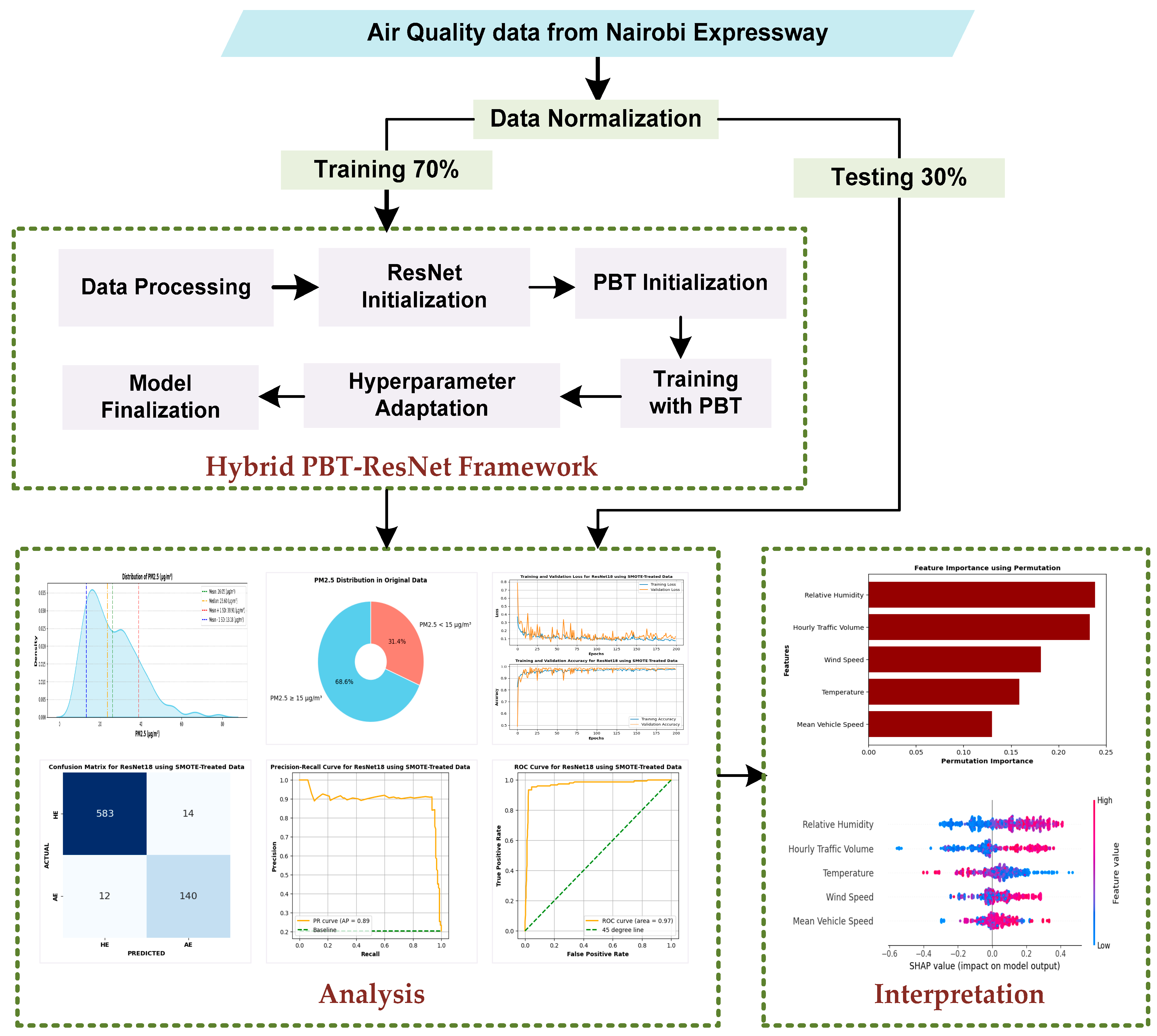Figure 1 depicts the proposed hybrid PBT-ResNet framework.

The remaining paper is structured as follows: Section 2 reviews existing literature on statistical, machine learning and deep learning strategies for PM2.5 prediction, showing their strengths and limitations. Section 3 describes the study location in detail and provides a theoretical overview of the hybrid PBT-ResNet framework, along with the performance metrics used to evaluate different models. Section 4 analyzes the dataset, evaluates the performance of various models, and presents a comparative analysis. This section also includes an interpretation of the optimal model. Finally, Section 5 concludes the study by summarizing key findings with limitations and recommendations for future research.

2. Related Work

The analysis of air quality in metropolitan landscapes has become a critical area of study due to its significant impact on public health and ecological balance. Among airborne pollutants, PM2.5 has gained particular attention because of its severe health risks, which are especially pronounced in densely populated areas. Numerous predictive studies have been developed to assess and forecast air quality trends with a specific focus on PM2.5 levels. Traditional statistical frameworks, such as Land Use Regression (LUR) [18,19], time series models including Auto-Regressive Integrated Moving Average (ARIMA), seasonal autoregressive integrated moving average (SARIMA) and FBProphet [20,21,22], and Generalized Additive Models (GAMs) [23] have demonstrated efficacy in providing spatial and short-term forecasts of PM2.5 levels across varied locales, including in the USA, Europe, Africa, and Asia. Nevertheless, these models are predicated on stringent assumptions regarding data characteristics, such as normality, linearity, homoscedasticity, and error independence. The violation of these assumptions frequently culminates in skewed or imprecise predictions.

Conversely, machine learning and deep learning frameworks eschew the need for rigid data distribution assumptions, rendering them inherently more versatile and adept at encapsulating intricate data patterns and interdependencies [24]. This adaptability enables these models to more effectively address the complexities and stochastic nature of real-world datasets, which are often characterized by nonconformity to theoretical distributions, noise, and idiosyncrasies. Advanced machine learning and deep learning algorithms such as Recurrent Neural Networks (RNNs) [25], Convolutional Neural Networks (CNNs) [26], Long Short-Term Memory (LSTM) [27,28], Extreme Gradient Boosting (XGBoost) [29,30] and Random Forest (RF) [31], etc., have been extensively deployed to forecast PM2.5 levels, based on their reliable capability in predictive modeling.

Table 1. Overview of Global Studies on PM2.5 estimation.

Model	Findings	Region	Ref.
Hybrid Regression Model (Combining Multiple Linear Regression and Time Series Analysis)	Identified meteorological factors such as temperature and humidity as significant predictors of PM2.5 concentrations.	Beijing, China	[32]
National Scale Land Use Regression (LUR) Model	Developed a spatio-temporal LUR model for PM2.5, PM10, and NO2 concentrations and identified key predictors such as satellite-derived aerosol optical depth (AOD), meteorological variables, and land use factors, achieving high spatial and temporal prediction accuracy	China	[33]
Statistical, Machine learning and Hybrid models	Spatial and temporal gaps were addressed via satellite-driven AOD products address in PM concentration estimation	Global	[34]
Multiple Linear Regression (Site-Specific Statistical Model)	Estimated ground-level PM2.5 due to wildfire smoke events using fire-related variables (FRP, fire danger indices), and smoke-related variables (AOD, smoke plume perimeters)	Western United States	[35]
Linear Mixed-Effect (LME) Model and Geographically Weighted Regression (GWR)	Addressed AOD data gaps using MERRA-2 AOD and developed an LME model coupled with GWR to estimate PM2.5 concentrations	Madhya Pradesh, India	[36]
Multiple Linear Regression (MLR) with Statistical Distribution Techniques	Predicted PM2.5 concentrations in non-monitored areas of Central Business District (CBD) in addition to GIS-based risk assessment	Bangkok, Thailand	[37]
Best Subset Regression, Random Subspace, Additive Regression, Reduced Error Pruning Tree, and Random Tree	Assessment of correlation of PM2.5 levels with precipitation, relative humidity, and temperature	Dhaka, Bangladesh	[38]
Geophysical Chemical Transport Models (CTMs), Interpolation Methods, Satellite-Derived Aerosol Optical Depth (AOD) Method, Bayesian Statistical Regression Model, and Machine Learning Methods	Broad consistency in PM2.5 concentration predictions across models, with higher levels observed in the eastern U.S. and greater variability in the western U.S. An average decrease of 1 µg/m3 in PM2.5 concentrations was projected between 2011 and 2028 due to emission reduction regulations.	United States	[39]
Extreme Gradient Boosting (XGBoost) and Fully Connected Neural Network (FCNN)	Analyzed the feature importance of meteorological variables, revealing their significant influence on PM2.5 concentrations.	Hunan Province, China	[40]
Random Forest combined with NASA’s GEOS-CF Chemical Transport Model (CTM)	Assessed PM2.5 concentrations with spatiotemporal continuity, reduced biases in GEOS-CF predictions, and provided 1 km resolution forecasts with minimal computational requirements	Central China	[41]
Weighted Long Short-Term Memory Neural Network Extended Model (WLSTME)	Addressed spatiotemporal dependencies and site density variations and showed consistent superior performance across all seasons and regions.	Beijing–Tianjin–Hebei Region, China	[42]
Random Forest (RF) and Support Vector Regression (SVR)	Estimated that PM2.5 concentrations were higher in urban/industrial areas compared to suburban/rural areas and peaked during the dry season (June–September)	Malaysia	[43]
Convolutional Neural Network (CNN) and Gated Recurrent Unit (GRU) with Geographical Polygon Group Model	Predicted PM2.5 concentrations at 25 stations with an index of agreement (IOA) of 0.82–0.89 and a Pearson correlation coefficient of 0.70–0.83.	Seoul, South Korea	[44]
Space–Time Extremely Randomized Trees	Observed air quality improvements across Europe during the study period, with further improvements during the COVID-19 lockdown, except in specific regions like the UK, Ireland, northern France, and southern Italy.	Europe	[45]

below shows a compilation of diverse studies focused on PM2.5 level estimation which employ a range of strategies, encompassing statistical frameworks, machine learning paradigms, and deep learning techniques.

To the best of our knowledge, existing models for PM2.5 estimation, including statistical, machine learning, and deep learning approaches, often exhibit certain limitations that hinder their performance and applicability. Statistical models are effective for short-term predictions and spatial analysis but rely on strict assumptions such as data normality, linearity, and homoscedasticity. These assumptions are often violated in real-world scenarios, which leads to biased or imprecise results. Machine learning models are flexible but require extensive hyperparameter tuning and may struggle to capture spatiotemporal dependencies effectively. Deep learning models have superior ability to learn complex patterns but are computationally expensive and lack interpretability.

Recognizing these shortcomings, we propose a hybrid PBT-ResNet framework, which integrates the robust predictive capabilities of ResNet with the adaptive hyperparameter optimization of PBT. This hybrid approach addresses the computational inefficiency and lack of adaptability seen in deep learning models by dynamically optimizing hyperparameters during training. Furthermore, ResNet’s layered architecture enables it to capture intricate relationships in the data, while PBT ensures the model performs consistently across varying datasets. By combining these strengths, our proposed model enhances prediction accuracy and provides a scalable solution for PM2.5 estimation in diverse and complex scenarios.

3. Materials and Methods

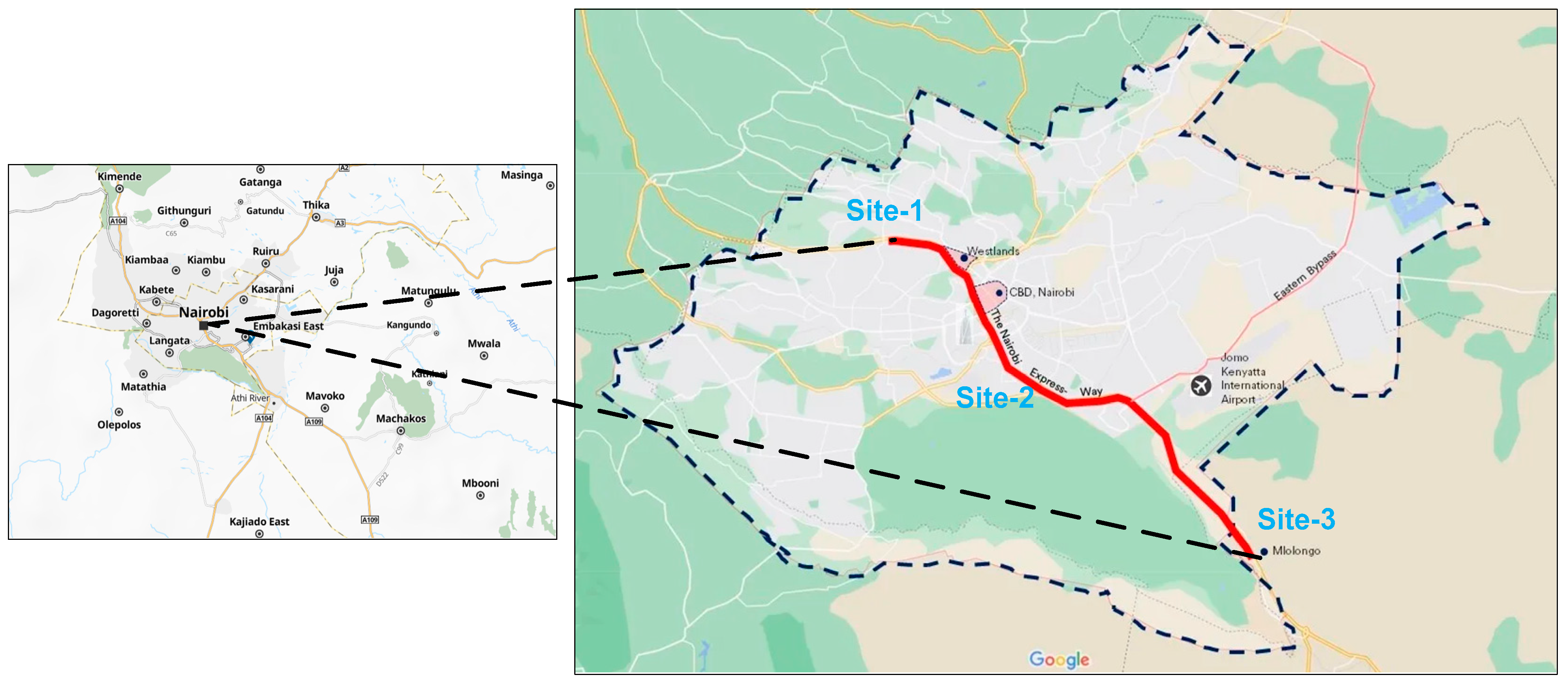
Air quality data for this study was obtained from three strategic locations along the Nairobi Expressway. The expressway is a 27 km (17-mile) dual six-lane carriageway designed to provide efficient high-capacity transit, strategically linking Nairobi’s Central Business District (CBD) with Jomo Kenyatta International Airport (JKIA). Starting at Mlolongo, the route follows Mombasa Road, continues along Uhuru Highway, and terminates at James Gichuru Road on Waiyaki Way. Key infrastructure features include toll stations, service lanes, and interchanges at major junctions. Serving daily commuters, airport travelers, and freight transport, the expressway plays a vital role in reducing congestion in the Nairobi metropolitan area.

3.1. Monitoring Site Details

To comprehensively assess air quality along the Nairobi Expressway, monitoring sensors were strategically installed at three key locations, as shown in Figure 2. These sites were selected to capture diverse traffic conditions, emission patterns, and meteorological influences across the corridor. The sensors included Open-Seneca air quality monitoring devices for measuring PM2.5, PM10, and gaseous pollutants such as NOx, SO₂, and CO. In addition, meteorological instruments were deployed to record temperature, humidity, and wind speed, critical for understanding pollutant dispersion dynamics.

3.1.1. Site 1: Westlands

Positioned near the western terminus of the expressway along Waiyaki Way, this site lies within a mixed commercial and residential zone. It serves as a critical junction connecting residential areas with commercial hubs. This location was chosen to analyze air quality variations caused by commuter traffic. Air quality sensors were deployed to capture localized emissions, focusing on changes in vehicular flow during peak and off-peak hours.

3.1.2. Site 2: Bellevue

Situated near the city center along Uhuru Highway within Nairobi’s CBD, this site combines residential and commercial land use. It was selected to evaluate the air quality impact of mixed traffic, including private vehicles, buses, and motorcycles, in a densely populated urban setting. Sensors were installed strategically to measure pollutants accurately, considering high traffic volumes and the urban heat island effect prevalent in this commercially vibrant region.

3.1.3. Site 3: Cabanas

Located near the eastern terminus of the expressway close to Mlolongo, this site represents a predominantly industrial and peri-urban area characterized by significant freight activity. It was chosen to monitor emissions from heavy commercial vehicles entering and exiting Nairobi and to evaluate their influence on nearby residential neighborhoods. Sensors were installed at a roadside elevation to capture detailed vehicular emissions and meteorological data, allowing the assessment of the impact of industrial traffic on local air quality.

3.2. Hybrid PBT-ResNet Framework

The Hybrid PBT-ResNet framework is a novel approach that combines ResNet with the adaptive hyperparameter optimization strength of PBT to classify PM2.5 concentrations. ResNet is a well-established deep learning architecture known for its ability to capture complex patterns through residual learning, making it particularly suited for high-dimensional and non-linear problems [46,47]. The integration of PBT allows for the dynamic optimization of critical hyperparameters during training, ensuring robust performance under varying environmental and traffic conditions. It is pertinent to mention that in this study, we evaluate three ResNet variants, ResNet18 [48], ResNet34 [49], and ResNet50 [50], to analyze the predictive performance of the framework across models with varying levels of complexity. This multi-scenario approach enables us to assess how model depth influences accuracy and reliability, allowing for the identification of the optimal architecture for precise PM2.5 levels classification. The working principle of hybrid PBT-ResNet framework is as follows.

3.2.1. Data Preprocessing

Let the dataset is represented by $D=\left\{X,Y\right\}$, where X represents features including meteorological and traffic data) and Y represents the PM2.5 levels. The input features are normalized using Equation (1).

$$X^{\prime }={\displaystyle \frac{X-\mathit{\mu }}{\mathit{\sigma }}}$$

(1)

where μ is the mean and σ is the standard deviation. In addition, the numerical values of PM2.5 levels are converted to categorical labels, in order to establish a binary classification problem as shown by Equation (2). The data are then split into training $\left(D_{\mathit{train}}\right)$ and test $\left(D_{\mathit{test}}\right)$ sets.

$$Y=\left\{\begin{array}{ll}1& \mathrm{if} \mathrm{PM}2.5 \mathrm{Levels} \ge 15 \mu \mathrm{g}/{\mathrm{m}}^3\\ 0& \mathrm{if} \mathrm{PM}2.5 \mathrm{Levels} < 15 \mu \mathrm{g}/{\mathrm{m}}^3\end{array}\right.$$

(2)

3.2.2. ResNet Model Initialization

The ResNet architecture with l layers and residual connection is defined by Equation (3).

$$H^{\left[l\right]}X=F^{\left[l\right]}X+X$$

(3)

where $F^{\left[l\right]}X$ is the transformation at layer l and $H^{\left[l\right]}X$ is the output. Initialize weights $W_l$ and biases $b_l$ for each layer l, using Xavier initialization [51]. Xavier initialization (Glorot Initialization) is a popular method for initializing neural network weights. It ensures that the weights are set such that the variance of inputs and outputs remains consistent across layers, minimizing issues like vanishing or exploding gradients [52].

3.2.3. PBT Initialization

The initialization phase of PBT for ResNet involves configuring a population of ResNet models, each with unique hyperparameter combinations specific to ResNet model architecture and training dynamics. These hyperparameters control both the structural design of ResNet and its optimization process during training. Let the population P consist of n ResNet models:

$$P=\left\{M_1\left({\theta }_1\right),M_2\left({\theta }_2\right),\dots ,M_n\left({\theta }_n\right)\right\}$$

(4)

where $M_i$ denotes the $i^{th}$ ResNet model and ${\theta }_i$ are the model-specific hyperparameters.

3.2.4. Training with PBT

Train each model $M_i$ in the population for a predefined interval T, using the objective function (cross-entropy loss) as illustrated by Equation (4). In this study, T is measured in epochs and represents the number of complete passes through the training dataset during a single training phase of the PBT process. The performance of each model is evaluated on $D_{val}$ using the classification accuracy metric.

$$\Gamma \left(Y,\widehat{Y}\right)=-{\displaystyle \frac{1}{N}}{\displaystyle \sum _{i=1}^N\left[Y_i\log \left({\widehat{Y}}_i\right)+\left(1-Y_i\right)\log \left(1-{\widehat{Y}}_i\right)\right]}$$

(5)

3.2.5. Hyperparameter Adaptation

The best model $\left(M_{opt}\right)$ is selected based on classification accuracy. To achieve this, the best models are cloned and fine-tune their hyperparameters slightly, and replace underperforming models with new hyperparameter configurations sampled randomly or through perturbation. The perturbation mechanism introduces small, controlled changes to the hyperparameters of the cloned models, enabling the exploration of diverse configurations while preserving the stability of the population. Key hyperparameters subjected to perturbation include the optimizer, activation function, learning rate, and weight decay, which are crucial for the performance and stability of the ResNet architecture.

3.2.6. Model Finalization

The best performing model $\left(M^{*}\right)$ in the population is identified after N iterations based on validation classification accuracy. The best model is retained on the combined training and validation set for optimal performance.

3.2.7. Prediction and Classification

The best-trained model is employed to predict PM2.5 labels for the testing dataset $\left(D_{test}\right)$ as shown by Equation (6). Then, each instance is classified based on the WHO guidelines as per Equation (2)

$$\widehat{Y}=\mathrm{Softmax}\left(H^{[L]}(X^{\prime })\right)$$

(6)

3.3. Competitive Classification Models

3.3.1. Feedforward Neural Network (FNN)

The FNN is a widely used deep learning model for predicting PM2.5 levels due to its ability to model non-linear relationships between input features and the target [53,54]. In the context of PM2.5 prediction, the FNN processes input data, such as meteorological and traffic related factors, through interconnected layers of neurons. Each layer applies transformations using weighted connections and activation functions to capture complex patterns within the data. By using historical PM2.5 data along with relevant predictors, an FNN can produce accurate forecasts of air quality, making it a valuable tool for pollution monitoring and management efforts.

3.3.2. Gene Expression Programming (GEP)

GEP is a widely used evolutionary computation technique for predicting complex phenomena, such as PM2.5 levels, due to its ability to model intricate non-linear relationships between input variables and output [55]. GEP evolves populations of candidate solutions through genetic operators like mutation, crossover, and selection, combining the strengths of genetic algorithms and genetic programming. This flexible methodology encodes mathematical models as chromosomes and decodes them into expression trees, enabling the discovery of interpretable, highly accurate relationships. The adaptability and efficiency of GEP make it a powerful tool for environmental modeling and air quality prediction tasks.

3.3.3. Bidirectional Long Short-Term Memory (BiLSTM)

BiLSTM networks are designed to capture dependencies in sequential data by processing information in both forward and reverse directions [56]. This bidirectional processing allows BiLSTM to employ both past and future context, making it particularly effective for PM2.5 forecasting tasks [57]. Through its gating mechanisms, which include input, forget, and output gates, BiLSTM can model long-term dependencies in air quality data without suffering from vanishing gradient issues. The ability to consider sequences bidirectionally enables BiLSTM to uncover intricate relationships between historical and future PM2.5 levels, ensuring accurate and reliable predictions.

3.3.4. Bidirectional Gated Recurrent Unit (BiGRU)

BiGRU networks utilize bidirectional processing to analyze sequences in both forward and reverse directions, enhancing their ability to capture temporal dependencies in PM2.5 forecasting [58]. BiGRU employs a simplified architecture compared to BiLSTM, relying on update and reset gates to control the flow of information. This streamlined structure reduces computational complexity while maintaining strong performance in modeling sequential patterns. The bidirectional nature of BiGRU ensures that it effectively captures both historical trends and future contexts, making it a powerful tool for air quality prediction tasks.

3.4. Performance Measures

This study evaluates the performance of various classification models for PM2.5 classification using key metrics: precision, recall, F1-Score, Matthews Correlation Coefficient (MCC), G-Mean, and Balanced Accuracy (BA). These metrics are derived from the confusion matrix components: True Positives (TPs), False Positives (FPs), False Negatives (FNs), and True Negatives (TNs). Precision measures the proportion of correctly identified HE instances (TPs) out of all predicted HE cases (TPs + FPs), reflecting the model’s ability to minimize FPs. Recall, on the other hand, evaluates the capability of the model to correctly identify AE instances (TPs) among all actual AE occurrences (TPs + FNs), focusing on minimizing FNs. The F1-Score combines precision and recall into a single metric by calculating their harmonic mean, providing a balance between FPs and FNs. MCC is a robust metric that evaluates the correlation between predicted and actual classifications, considering all components of the confusion matrix (TPs, FPs, FNs, TNs). It is particularly effective for imbalanced datasets, as it provides a balanced evaluation. G-Mean assesses the balance between sensitivity (recall) and specificity (the ability to correctly identify TNs), ensuring consistent performance across both positive and negative classes. Finally, BA, which is the average of class-specific recall rates, accounts for class imbalance by equally weighing the performance of both classes. The mathematical formulations for these metrics are provided in Equations (7)–(11).

$$\mathrm{Precision}={\displaystyle \frac{\mathit{TP}}{\mathit{TP}+\mathit{FP}}}$$

(7)

$$\mathrm{Recall}={\displaystyle \frac{\mathit{TP}}{\mathit{TP}+\mathit{FN}}}$$

(8)

$$\mathrm{G}-\mathrm{M}\mathrm{e}\mathrm{a}\mathrm{n}=\sqrt{\left({\displaystyle \frac{\mathit{TP}}{\mathit{TP}+\mathit{FN}}}\right)\left({\displaystyle \frac{\mathit{TN}}{\mathit{FP}+\mathit{TN}}}\right)}$$

(9)

$$\mathrm{BA}={\displaystyle \frac{1}{2}}\left({\displaystyle \frac{\mathit{TP}}{\mathit{TP}+\mathit{FN}}}+{\displaystyle \frac{\mathit{TN}}{\mathit{TN}+\mathit{FP}}}\right)$$

(10)

$$\mathrm{MCC}={\displaystyle \frac{\mathit{TP}\times \mathit{TN} - \mathit{FP}\times \mathit{FN}}{\sqrt{\left(\mathit{TP}+\mathit{FP}\right)\left(\mathit{TP}+\mathit{FN}\right)\left(\mathit{TN}+\mathit{FP}\right)\left(\mathit{TN}+\mathit{FN}\right)}}}$$

(11)

4. Results and Discussion

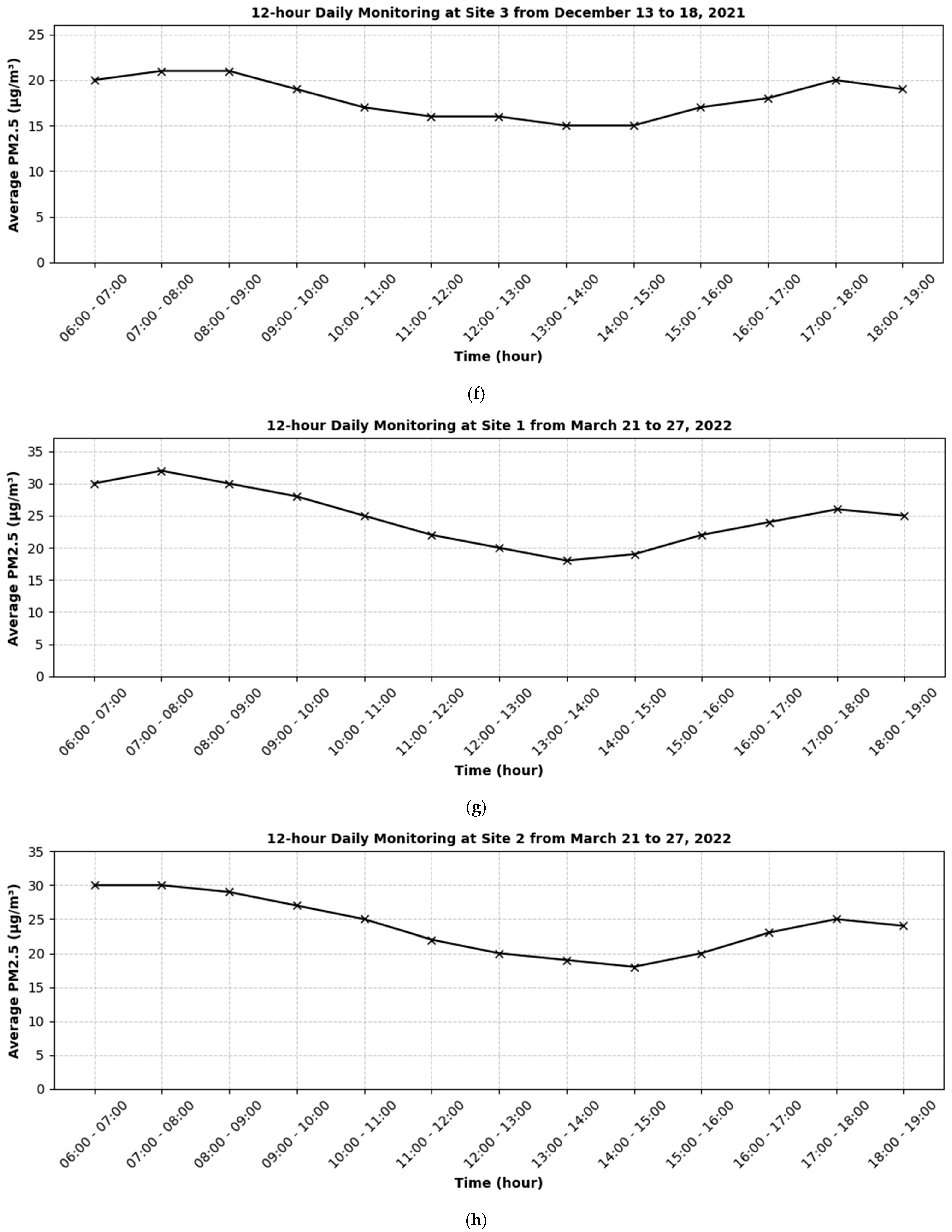
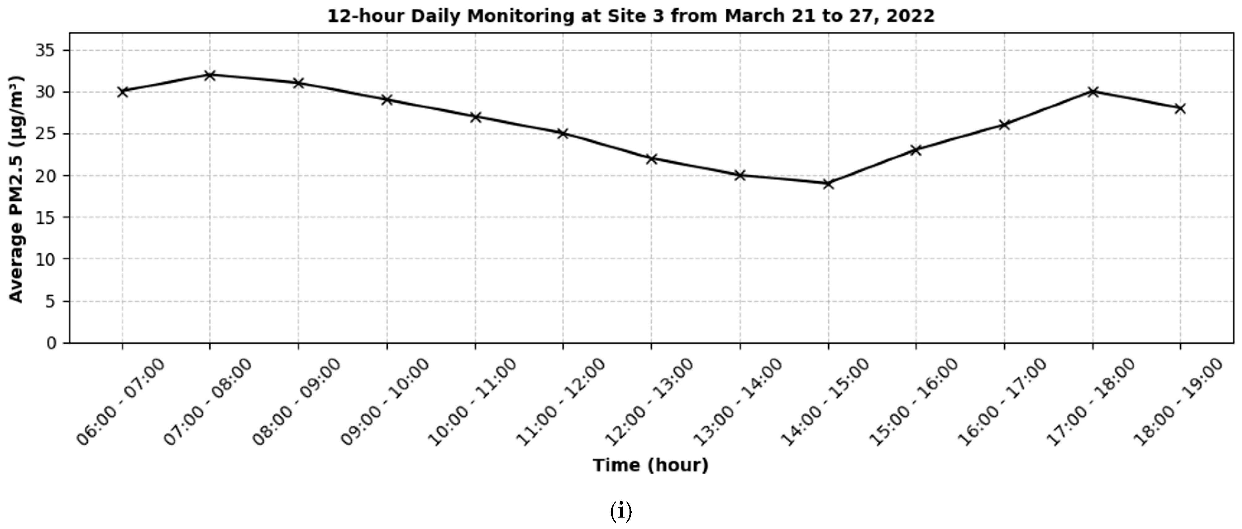
In this study, data were collected at three strategically selected locations along the Nairobi Expressway corridor, as discussed in Section 3.1, with monitoring conducted daily for 12 h (06:00–18:00) over seven consecutive days. Observations were focused on peak traffic periods to capture maximum vehicular emissions and their impact on ambient air quality. To account for seasonal variability in PM2.5 levels, data were collected during three distinct temporal windows: 23–29 August 2021 (dry season), 13–18 December 2021 (peak holiday season), and 21–27 March 2022 (post-holiday dry period). August represents the dry season in the region, characterized by the absence of precipitation, which intensifies dust suspension and amplifies PM2.5 levels. The peak holiday season is marked by increased traffic volumes and their emissions, further exacerbating air quality conditions. In contrast, the post-holiday dry period provides a window to assess typical daily traffic patterns and ambient air quality under non-peak travel conditions. In addition to pollutant concentration data, the study also recorded hourly traffic volumes (veh/h), mean vehicle speed (km/h), and meteorological parameters, including relative humidity (%), wind speed, and temperature (°C).

Table 2. Sample data from different locations along the Nairobi Expressway.

Date and Time	PM2.5 (µg/m3)	Relative Humidity (%)	Hourly Traffic Volume (veh/h)	Wind Speed (m/s)	Temperature (°C)	Mean Vehicle Speed (km/h)
24/08/2021 @ 09:45 (Site 1)	45.2	73	943	5.6	25.3	45.6
26/08/2021 @ 14:30 (Site 2)	36.3	46	1240	4.6	27.4	56.1
-	-	-	-	-	-	-
-	-	-	-	-	-	-
15/12/2021 @ 15:00 (Site 2)	50.1	35	1120	5.2	19.47	48.9
17/12/2021 @ 12:40 (Site 3)	33.8	42	980	5.8	20.47	58.3
	-	-	-	-	-
	-	-	-	-	-	-
23/03/2022 @ 17:30 (Site 1)	46.7	32	1300	5	24.4	46.3
27/03/2022 @ 10:25 (Site 3)	38.3	28	1422	3.9	22.8	53.7

illustrates a sample of the data collected along the expressway.

Figure 3 illustrates the 12 h daily monitoring of PM2.5 concentrations across various sites and time periods. For each site, there is a discernible pattern where PM2.5 levels tend to peak during the early morning hours (06:00–09:00) and again during the late afternoon to early evening hours (16:00–19:00). This trend shows possible links to rush-hour traffic and human activity, as these time frames often coincide with increased vehicle emissions and other pollutant sources. Moreover, the midday periods (10:00–15:00) generally show a decline in PM2.5 levels across most sites.

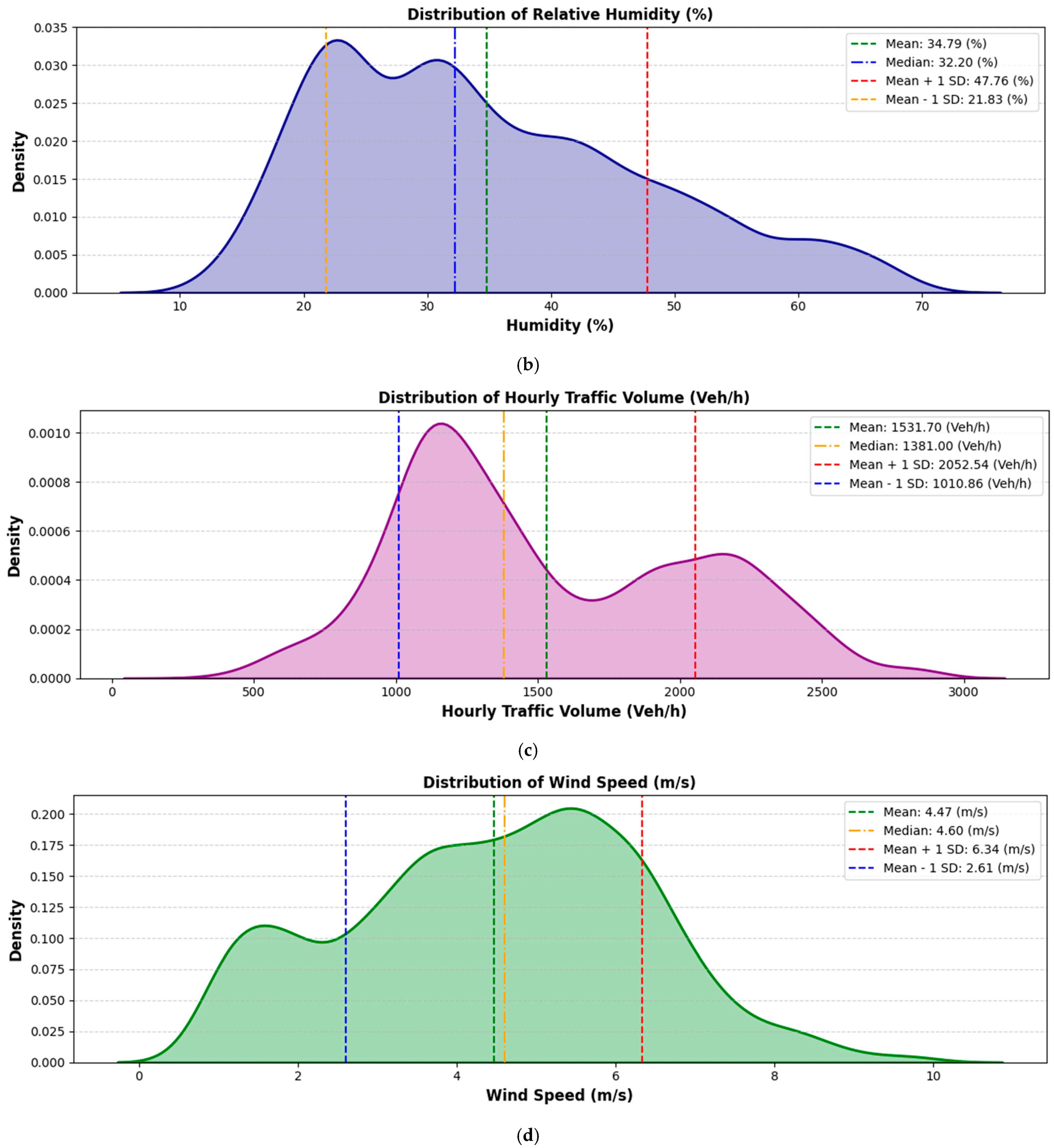
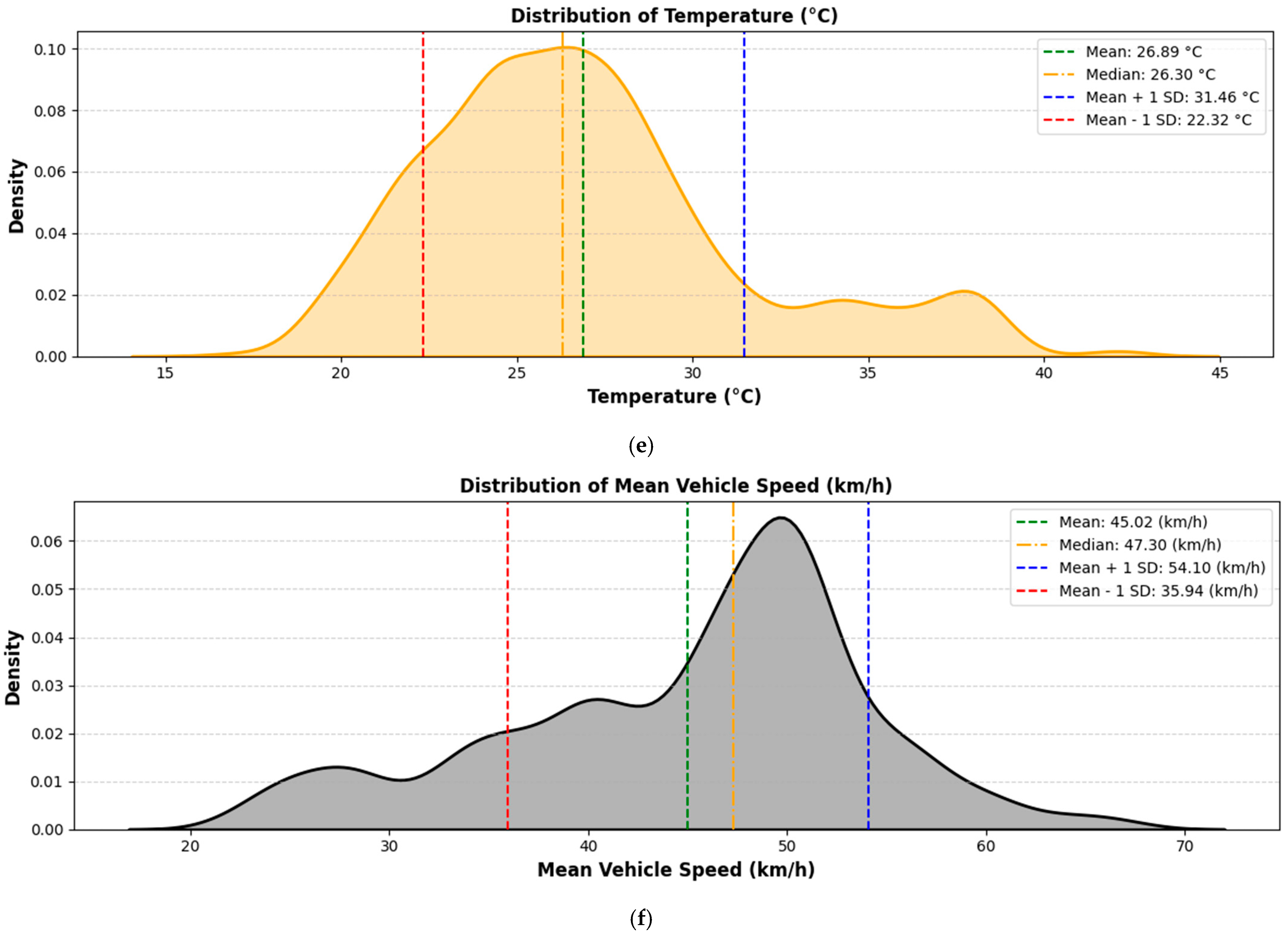
In addition, the density plots of different parameters provide a clear depiction of the distributions for various environmental and traffic parameters monitored along the study corridor, as shown in Figure 4. The PM2.5 levels have a mean value of 26.05 µg/m³ and a median of 23.60 µg/m³, with a standard deviation of 7.04 µg/m³. The distribution is wide, indicating occasional spikes likely influenced by traffic and weather conditions. The humidity factor, with a mean of 34.79%, a median of 32.20%, and a standard deviation of 11.97%, shows relative stability, with values mostly centered around the mean and occasional increases. Hourly traffic volume exhibits significant variability, with an average of 1531.70 veh/h, a median of 1381.00 veh/h, and a standard deviation of 520.38 veh/h. The wind speed parameter, with a mean of 4.47 m/s, a median of 4.60 m/s, and a standard deviation of 1.87 m/s, reflects generally consistent conditions with only occasional stronger winds. The temperature averaging 26.89 °C with a median of 26.30 °C and a standard deviation of 4.59 °C, displays a balanced distribution, indicating steady climatic conditions during the study. Similarly, the average vehicle speed is 45.02 km/h, with a median of 47.30 km/h and a standard deviation of 9.72 km/h, showing that most vehicles maintained speeds close to this value with some fluctuation.

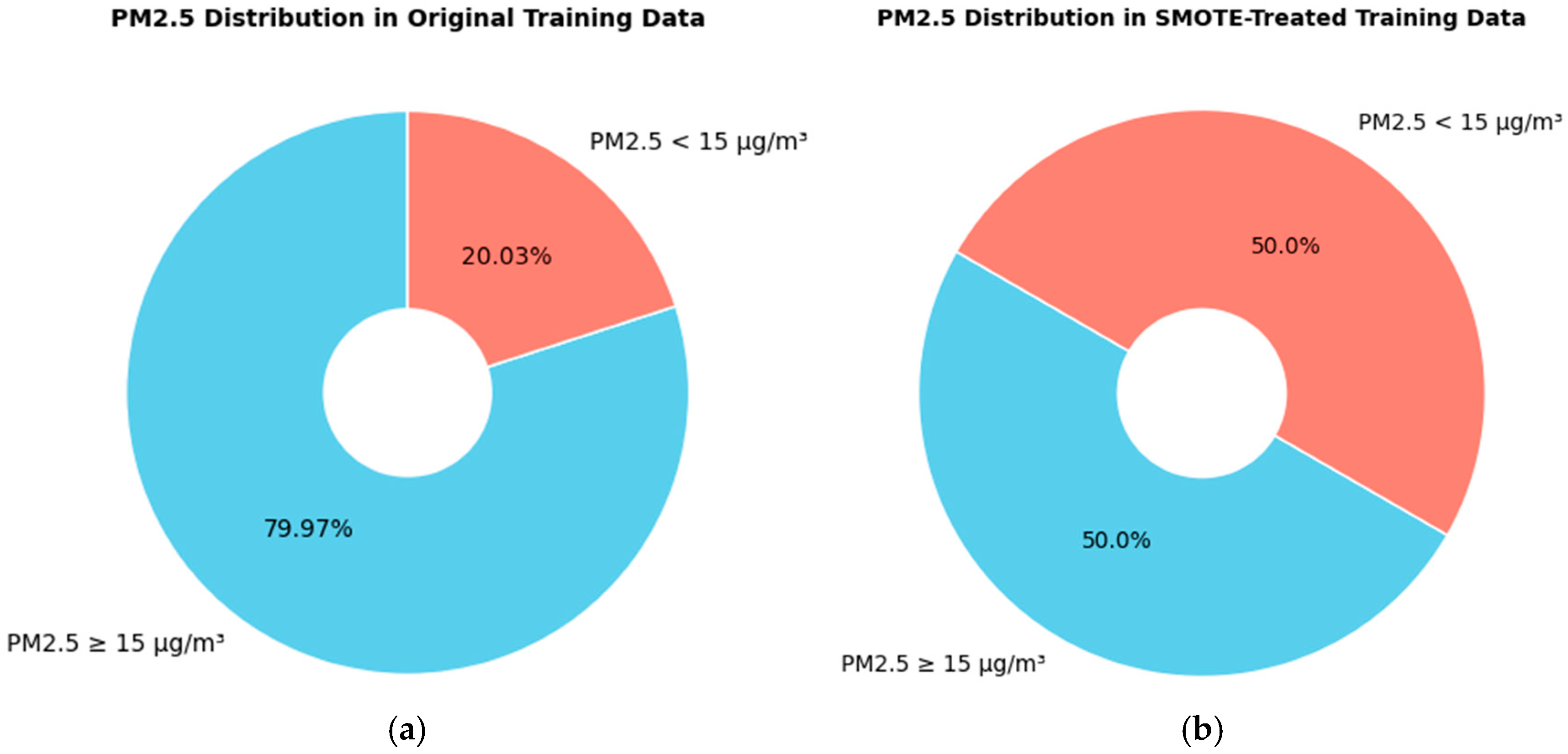
4.1. Data Imbalance and SMOTE Application

In this study, the dataset was divided into training and testing sets using a 70:30 split. A binary classification problem was framed to predict air quality classifications based on PM2.5 levels, following WHO guidelines. Instances with PM2.5 concentrations ≥ 15 µg/m³ were classified as Class 1 (hazardous exposure, HE), while those with concentrations < 15 µg/m³ were categorized as Class 0 (acceptable exposure, AE). The original dataset contained 2496 instances, comprising 1996 HE instances (79.97%) and 500 AE instances (20.03%), as shown in Figure 5a. This imbalance risked creating biased model predictions favoring the majority class. The training set included 350 AE instances and 1397 HE instances, while the test set comprised 150 AE instances and 599 HE instances. To mitigate the imbalance in the training set, the Synthetic Minority Oversampling Technique (SMOTE) was applied, yielding a balanced dataset with 1397 instances in each class (50%), as illustrated in Figure 5b.

4.2. Hyperparameters Tuning via PBT

Hyperparameter tuning is crucial for achieving optimal performance in deep learning models. In this study, PBT was employed as the optimization strategy to dynamically adjust hyperparameters during training. PBT enables both exploration and exploitation of the hyperparameter space, allowing ResNet models to adapt to varying data patterns and improve accuracy. The key hyperparameters considered for tuning, along with their descriptions, are summarized in

Table 3. Description of ResNet Model Hyperparameters.

Hyperparameters	Description
Optimizer	PBT enables the selection and evolution of optimizers throughout training, dynamically switching between algorithms such as Adam, SGD, or RMSprop. The choice of optimizer influences the convergence speed and stability of the model.
Activation Function	Activation functions introduce non-linearity into the model, enabling it to learn complex patterns. Commonly used activation functions in ResNet include ReLU, which mitigates the vanishing gradient problem.
Learning Rate	The learning rate is a critical hyperparameter that controls the step size for weight updates during back-propagation.
Weight Decay	Weight decay (L2 regularization) prevents overfitting by penalizing large weight magnitudes.

. The hyperparameters were tuned within predefined ranges to suit the architectural and computational requirements of ResNet18, ResNet34, and ResNet50, as detailed in

Table 4. Range of Hyperparameters for different ResNet models.

Hyperparameter	Range
Optimizer	Adam, SGD, RMSprop
Activation Function	ReLU, Leaky ReLU, GELU
Learning Rate	0.0001–0.01
Weight Decay	0.0001–0.001

.

PBT tuning determined the optimal hyperparameters for ResNet18, ResNet34, and ResNet50, as summarized in

Table 5. Optimal hyperparameters for different ResNet models.

Hyperparameter	ResNet18	ResNet34	ResNet50
Optimizer	Adam	SGD	RMSprop
Activation Function	ReLU	Leaky ReLU	GELU
Learning Rate	0.001	0.01	0.0005
Weight Decay	0.0001	0.0001	0.0005

. For ResNet18, the tuning process identified the Adam optimizer, the ReLU activation function, a learning rate of 0.001, and a weight decay of 0.0001, which align with its relatively shallow architecture and ability to focus on localized feature extraction. For ResNet34, the SGD optimizer with momentum, the Leaky ReLU activation function, a learning rate of 0.01, and a weight decay of 0.0001 were found to be optimal, reflecting its deeper architecture and enhanced capacity to capture complex patterns. For ResNet50, PBT tuning selected the RMSprop optimizer, the GELU activation function, a learning rate of 0.0005, and a weight decay of 0.0005, which cater to the demands of its substantial depth and high parameter count.

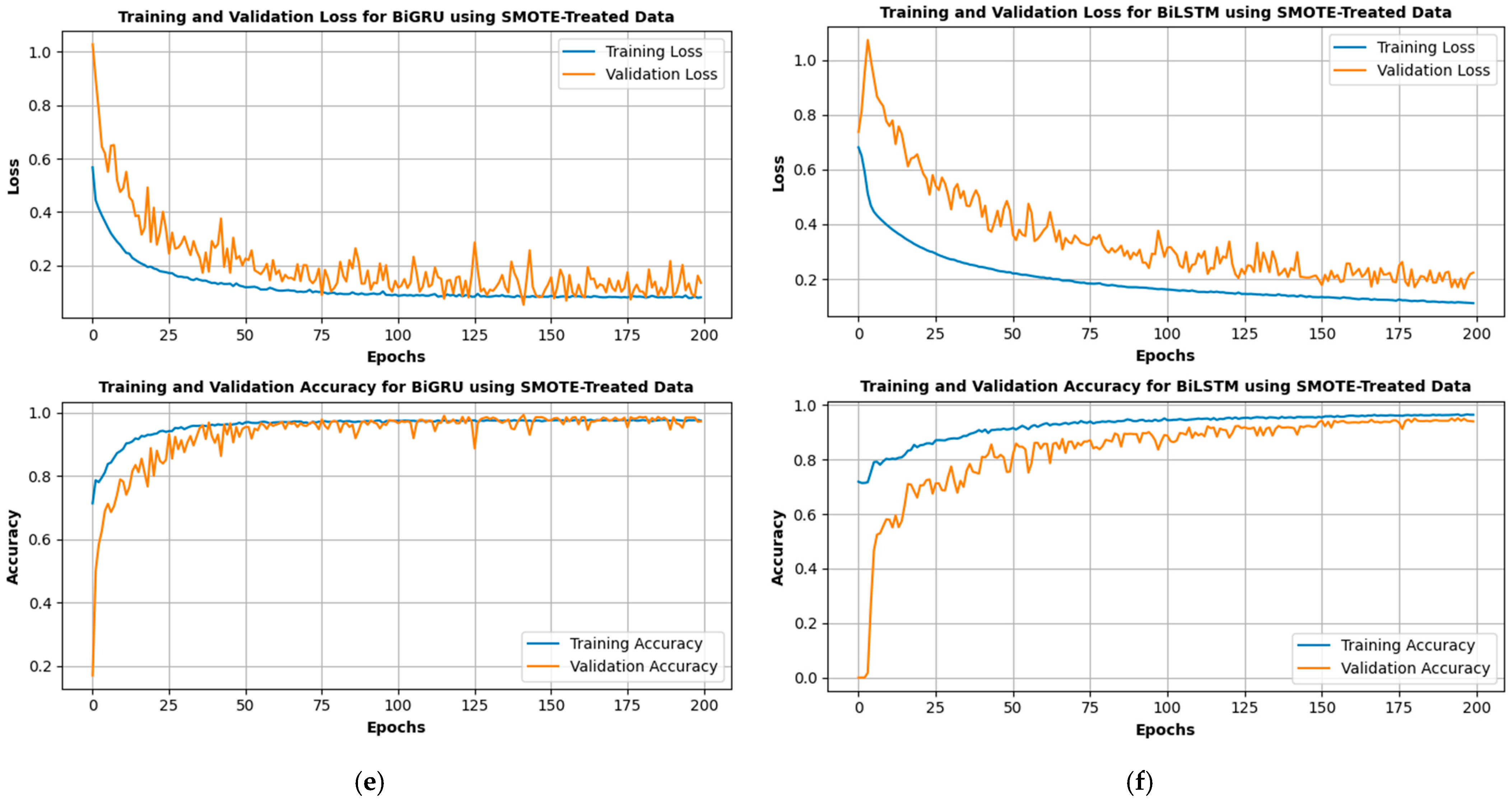
Based on the optimal hyperparameters, the final training and validation curves for ResNet18, ResNet34, ResNet50, FNN, BiLSTM, and BiGRU on SMOTE-treated data, as shown in Figure 6, Figure 7 and Figure 8, demonstrate varying convergence behaviors across the models. For ResNet18 and ResNet34, the training and validation losses decrease steadily over 200 epochs, stabilizing at low values, indicating effective learning with minimal overfitting. The training and validation accuracy curves approach high values, with ResNet34 achieving slightly higher accuracy than ResNet18, reflecting its deeper architecture’s capacity to extract more complex patterns. ResNet50 outperforms both, showing the lowest training and validation losses and the highest accuracy exceeding 0.9, showing its effectiveness in handling more complex data due to its greater depth. The FNN and BiLSTM models exhibit slower convergence compared to the ResNet architectures. While the training loss decreases significantly in both, the validation loss stabilizes at relatively higher values, indicating reduced generalization compared to ResNet models. The validation accuracy for FNN remains lower than that of the ResNet models, while BiLSTM shows improved accuracy but still falls short of ResNet50. BiGRU demonstrates competitive performance, with training and validation losses decreasing steadily and stabilizing at low values. The validation accuracy for BiGRU surpasses that of FNN and BiLSTM, and approaches close to ResNet50.

4.3. Performance Assessment of the Models

The performance of the proposed ResNet models and other competitive models in classifying PM2.5 as either HE or AE is illustrated using the confusion matrix, Receiver Operating Characteristic (ROC) curve, and Precision–Recall (PR) Curve in Figure 7.

4.3.1. Performance of ResNet18

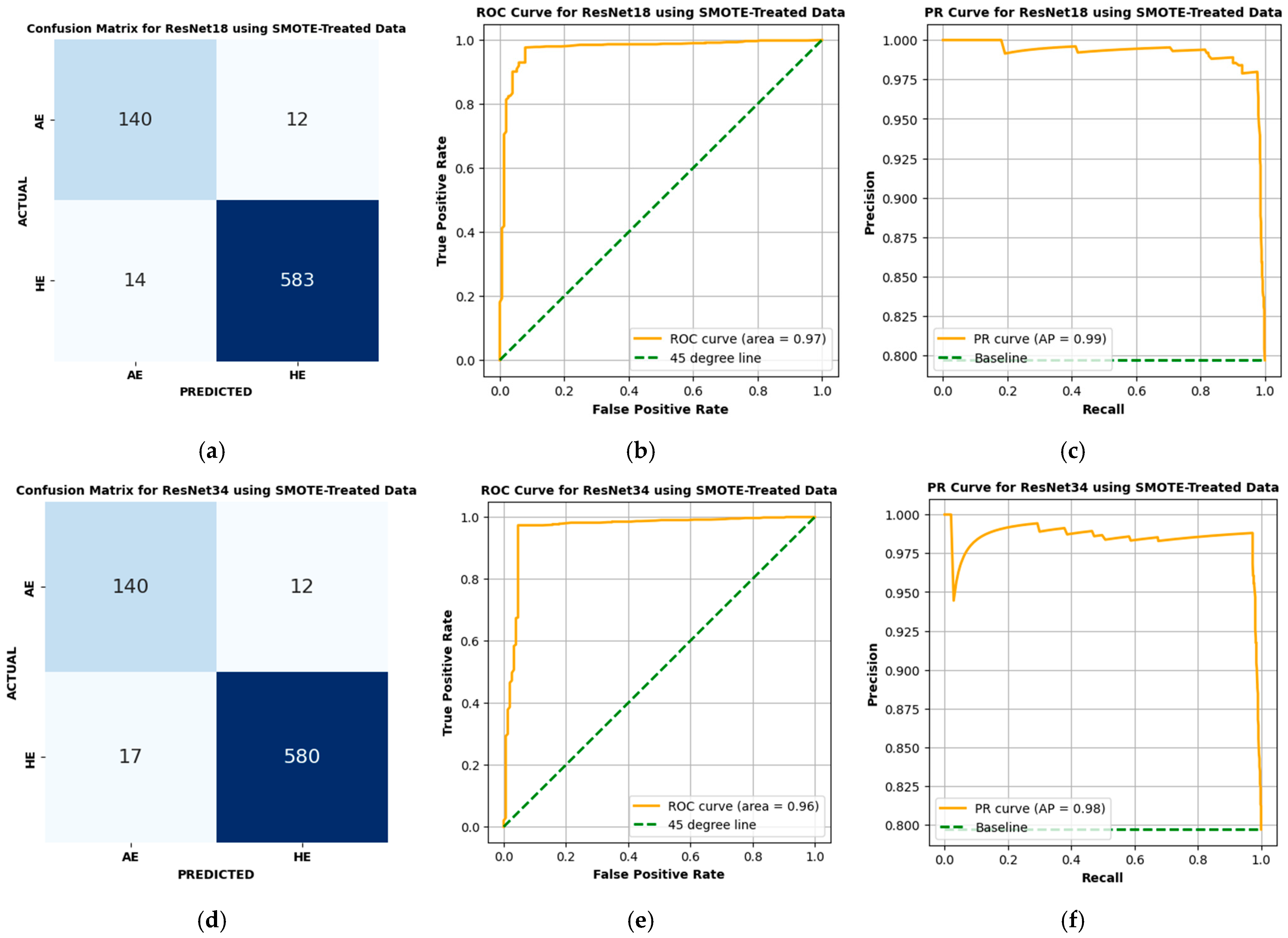
The ResNet18 Variant 1 model demonstrates remarkable performance in classifying HE and AE events using SMOTE-treated data. The confusion matrix, shown in Figure 7a, indicates that the model correctly classified 583 HE cases and 140 AE cases, while only misclassifying 14 HE cases as AE and 12 AE cases as HE. The ROC curve in Figure 7b illustrates the model’s strong capability to distinguish between HE and AE, achieving a high AUC of 0.97. Similarly, the PR curve in Figure 7c demonstrates an AP score of 0.99, reflecting the model’s effectiveness in maintaining a balance between precision and recall.

Table 6. Performance Measures of different models in classifying PM2.5.

Model	Precision	Recall	F1 Score	MCC	G-Mean	BA
ResNet18 (Variant 1)	0.979	0.976	0.978	0.893	0.948	0.948
ResNet34 (Variant 2)	0.988	0.971	0.979	0.904	0.962	0.962
ResNet50 (Variant 3)	0.979	0.963	0.971	0.863	0.941	0.942
FNN (baseline)	0.911	0.894	0.902	0.538	0.767	0.776
BiGRU (Baseline)	0.971	0.978	0.975	0.875	0.932	0.933
BiLSTM (Baseline)	0.961	0.969	0.965	0.828	0.907	0.909
GEP (Baseline)	0.910	0.5779	0.707	0.284	0.669	0.677

presents detailed performance metrics for the ResNet18 Variant 1 model, including a precision of 0.979, recall of 0.976, F1-score of 0.978, MCC of 0.893, G-Mean of 0.948, and BA of 0.948. These results establish ResNet18 Variant 1 as a reliable model for HE and AE classification, providing accurate predictions with minimal errors across all evaluation criteria.

4.3.2. Performance of ResNet34

ResNet34 Variant 2 demonstrates its effectiveness in classifying HE and AE events when applied to SMOTE-treated data. The confusion matrix in Figure 7d indicates that the model correctly identified 580 HE cases and 140 AE cases, with only 17 HE cases misclassified as AE and 12 AE cases misclassified as HE. The ROC curve in Figure 7e achieves an AUC of 0.96, indicating a strong ability to distinguish between the two classes. In addition, the PR curve in Figure 7f shows an AP score of 0.98, reflecting its capability to maintain precision and recall across different thresholds. Similarly, as shown in Table 6, ResNet34 Variant 2 achieves a precision of 0.988, recall of 0.971, F1-score of 0.979, MCC of 0.904, G-Mean of 0.962, and a BA of 0.962. Compared to ResNet18 Variant 1, ResNet34 Variant 2 provides improved precision and an improved F1-score, reducing FPs more effectively. However, ResNet18 outperforms slightly in recall and G-Mean, indicating better sensitivity to AE classifications. Both models achieve high performance, with ResNet34 excelling in precision and F1-score, while ResNet18 demonstrates slightly better recall and sensitivity. These distinctions may guide the selection of a model depending on the specific application requirements.

4.3.3. Performance of ResNet50

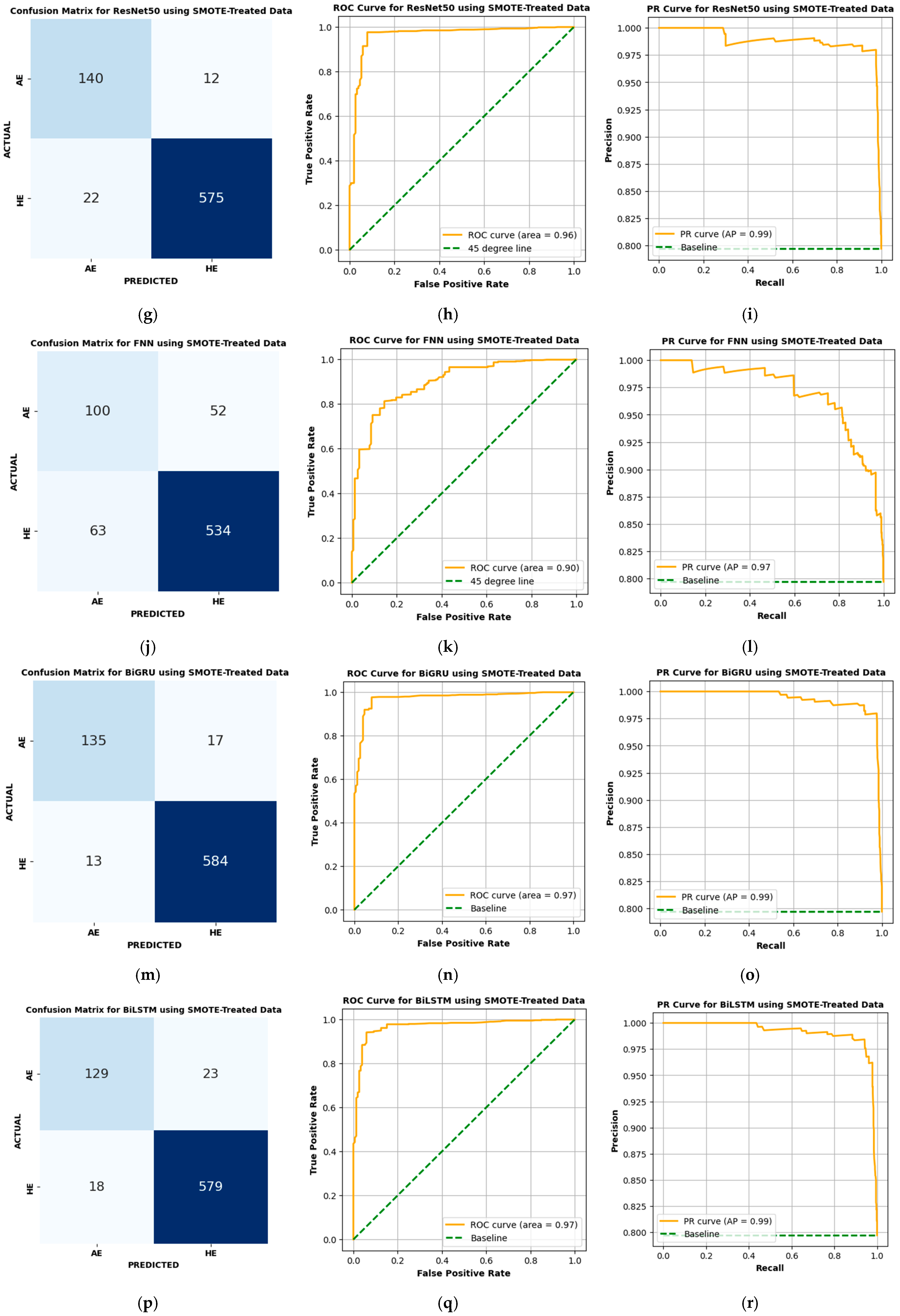
ResNet50 Variant 3 achieves competitive performance in classifying HE and AE events with SMOTE-treated data. Figure 7g reveals the confusion matrix, where the model correctly identified 575 HE cases and 140 AE cases, while misclassifying 22 HE cases as AE and 12 AE cases as HE. The ROC curve in Figure 7h shows an AUC of 0.96, showing an effective differentiation between the two classes. Furthermore, the PR curve in Figure 7i achieves an AP score of 0.99, reflecting its strong handling of precision and recall trade-offs across varying thresholds. As detailed in Table 6, the ResNet50 Variant 3 model attains a precision of 0.979, recall of 0.963, F1-score of 0.971, MCC of 0.863, G-Mean of 0.941, and a BA of 0.942. In comparison with ResNet34 Variant 2, ResNet50 demonstrates slightly lower recall and G-Mean but achieves a comparable F1-score and MCC, indicating consistent performance in classification tasks. While ResNet34 performs slightly better in detecting AE events, ResNet50 achieves balanced precision and recall, minimizing FPs effectively.

4.3.4. Performance of FNN

The FNN model, serving as a baseline for classifying HE and AE events, shows reasonable performance on SMOTE-treated data. Figure 7j provides the confusion matrix, showing that the model correctly classified 534 HE cases and 100 AE cases, but with a notable number of errors, including 63 HE cases misclassified as AE and 52 AE cases misclassified as HE. The ROC curve in Figure 7k reports an AUC of 0.90, reflecting its ability to distinguish between the two classes, though this value is lower than that achieved by the ResNet models. The PR curve in Figure 7l achieves an AP score of 0.97, reflecting a strong balance between precision and recall. Table 6 outlines the performance metrics for the FNN, including a precision of 0.911, recall of 0.894, F1-score of 0.902, MCC of 0.538, G-Mean of 0.767, and BA of 0.776. Compared to ResNet architectures, the FNN model performs less effectively, particularly in terms of MCC and G-Mean, illustrating its reduced ability to classify AE events accurately. The higher number of FNs (52, compared to 12 for ResNet18 and 7 for ResNet34) further indicates its limitations in sensitivity.

4.3.5. Performance of BiGRU

The BiGRU model also exhibits better performance in classifying HE and AE events using SMOTE-treated data, achieving competitive results compared to ResNet variants. The confusion matrix, shown in Figure 7m, indicates that BiGRU correctly classified 584 HE cases and 135 AE cases, while misclassifying 13 HE cases as AE and 17 AE cases as HE. The ROC curve in Figure 7n reports an AUC of 0.97, matching ResNet18 and outperforming ResNet34 (0.96) and ResNet50 (0.96). The PR curve in Figure 7o achieves an AP score of 0.99, aligning with ResNet50 and exceeding ResNet18 (0.89) and ResNet34 (0.98).

From Table 6, BiGRU achieves a precision of 0.971, recall of 0.978, F1-score of 0.975, MCC of 0.875, G-Mean of 0.932, and a BA of 0.933. Compared to ResNet18, BiGRU achieves a slightly lower precision (0.971 vs. 0.979) but a higher recall (0.978 vs. 0.976), resulting in comparable F1-scores (0.975 vs. 0.978). BiGRU also has a marginally lower MCC (0.875 vs. 0.893) and G-Mean (0.932 vs. 0.948). Against ResNet34, BiGRU outperforms in recall (0.978 vs. 0.971) but trails in precision (0.971 vs. 0.988) and MCC (0.875 vs. 0.904), while their F1-scores remain similar. When compared to ResNet50, BiGRU achieves matching AP (0.99) and recall (0.978 vs. 0.963) but falls slightly behind in precision (0.971 vs. 0.979), F1-score (0.975 vs. 0.971), MCC (0.875 vs. 0.904), and BA (0.933 vs. 0.942).

4.3.6. Performance of BiLSTM

The BiLSTM model delivers effective performance in classifying HE and AE events using SMOTE-treated data, as shown in Figure 7p–r. The confusion matrix in Figure 7p shows that the model accurately identified 579 HE cases and 129 AE cases, while misclassifying 18 HE cases as AE and 23 AE cases as HE. The ROC curve in Figure 7q achieves an AUC of 0.97, aligning with ResNet18, ResNet34, ResNet50, and BiGRU, indicating its strong capability to separate the two classes. The PR curve in Figure 7r achieves an AP score of 0.99, matching the performance of BiGRU and ResNet50, and surpassing ResNet18 (0.89) and ResNet34 (0.98). Table 6 provides detailed performance metrics for BiLSTM, which include a precision of 0.961, recall of 0.969, F1-score of 0.965, MCC of 0.828, G-Mean of 0.907, and BA of 0.909. When compared to ResNet18, BiLSTM falls short in precision (0.961 vs. 0.979) and F1-score (0.965 vs. 0.978), but achieves comparable recall (0.969 vs. 0.976). Against ResNet34, BiLSTM achieves similar recall (0.969 vs. 0.971) but is slightly behind in precision (0.961 vs. 0.988) and F1-score (0.965 vs. 0.979). ResNet50 continues to lead overall, outperforming BiLSTM in precision (0.979 vs. 0.961), recall (0.963 vs. 0.969), and F1-score (0.971 vs. 0.965). BiGRU, however, achieves better metrics across all categories compared to BiLSTM, including precision (0.971 vs. 0.961), recall (0.978 vs. 0.969), and F1-score (0.975 vs. 0.965).

4.3.7. Performance of GEP

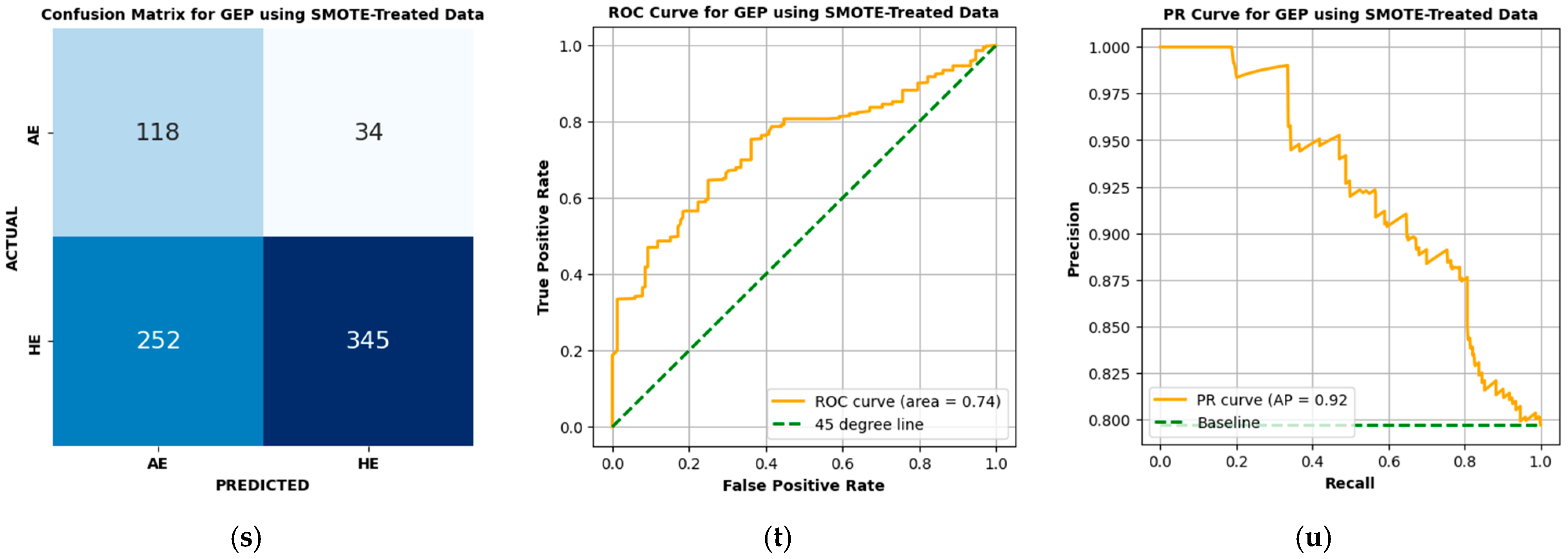
The GEP model exhibits limited performance in classifying HE and AE events using SMOTE-treated data. The confusion matrix in Figure 7s shows that GEP correctly classified 345 HE cases and 118 AE cases, while misclassifying 252 HE cases as AE and 34 AE cases as HE. The ROC curve in Figure 7t reports an AUC of 0.74, indicating a weaker ability to differentiate between the two classes compared to other models. The PR curve in Figure 7u achieves an AP score of 0.92, reflecting reasonable precision–recall performance but still lagging behind more advanced architectures. Table 6 shows the GEP model’s performance metrics, which include a precision of 0.910, recall of 0.578, F1-score of 0.707, MCC of 0.284, G-Mean of 0.669, and BA of 0.677. These results make GEP the weakest model among those evaluated. In comparison to FNN, GEP achieves higher precision (0.910 vs. 0.911) but falls significantly short in recall (0.578 vs. 0.894), leading to a much lower F1-score (0.707 vs. 0.902). Similarly, when compared to BiGRU and ResNet models, metrics of GEP are markedly inferior, with ResNet50 achieving precision, recall, and BA values consistently exceeding 0.94. The GEP model’s high FP count (252) heavily impacts its precision, while its moderate FN count (34) limits its recall.

4.4. Interpretation of Optimal ResNet34 Model

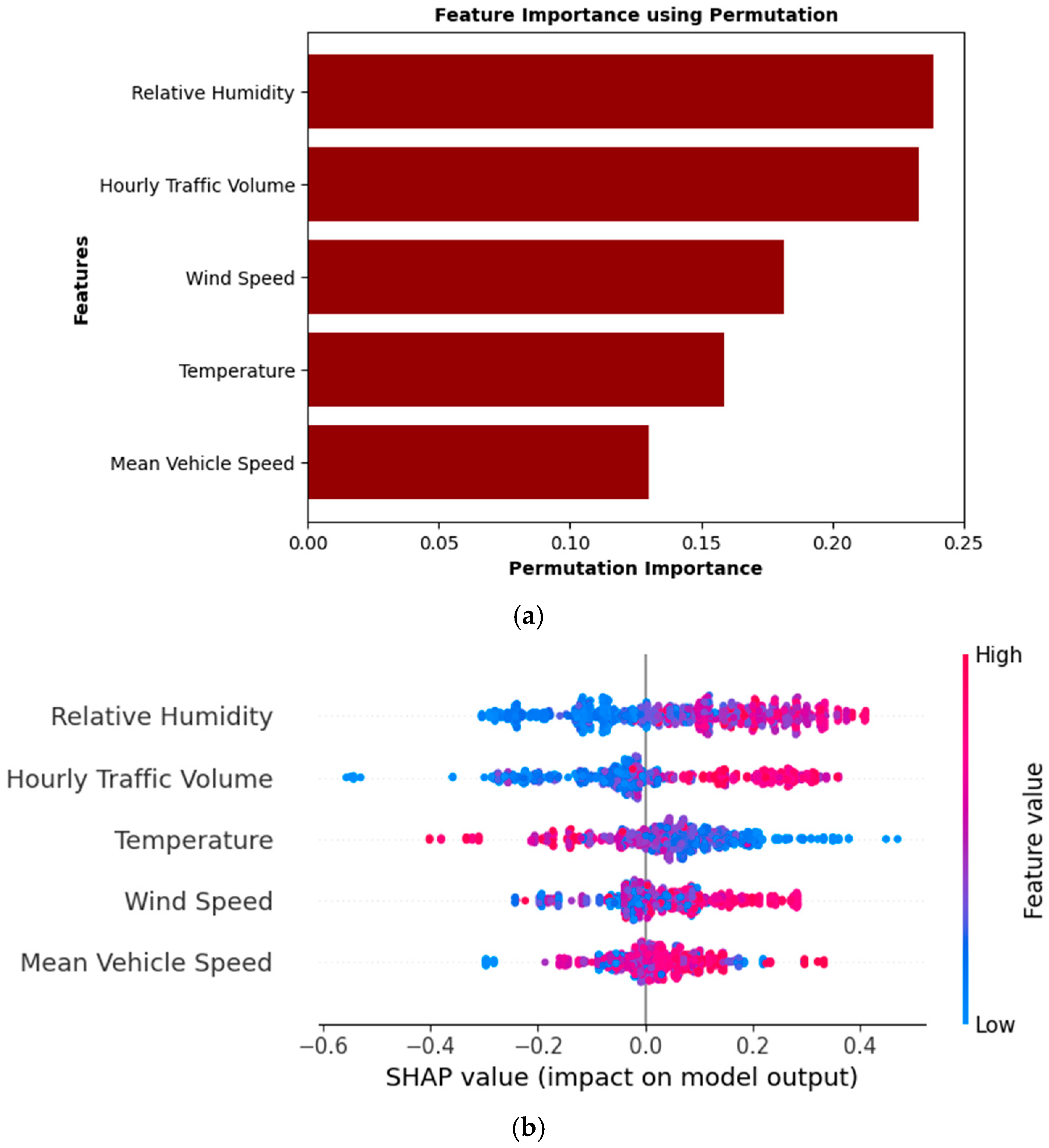
The feature importance analysis for the optimal ResNet34 model shows the factors influencing PM2.5 classification, as illustrated in Figure 8a,b. According to the permutation importance analysis in Figure 8a, the top contributing factor is relative humidity, followed by Hourly Traffic Volume, Wind Speed, Temperature, and Mean Vehicle Speed. The high permutation importance of relative humidity indicates its significant role in the model’s predictions, where changes in this feature have a considerable impact on classification outcomes.

The SHAP summary plot in Figure 8b provides valuable insights into the direction and magnitude of each feature’s impact on the output of the ResNet34 model. The relative humidity significantly influences PM2.5, with medium to high humidity levels (depicted by red and purple points) positively affecting the likelihood of HE events. This phenomenon occurs due to the hygroscopic behavior of particles, where increased moisture in humid conditions promotes particle growth and aggregation, making them more prominent in the environment. Conversely, lower humidity levels (blue points) inhibit particle growth, which is consistent with a higher probability of AE events. The hourly traffic volume is identified as another critical factor influencing the prediction of the ResNet34 model. Higher traffic volumes (red points) are strongly associated with an increased likelihood of HE events, likely resulting from elevated emissions caused by idling or slow-moving vehicles during traffic congestion. These results show the localized impact of traffic density on air quality along the Nairobi Expressway corridor, where vehicle congestion contributes significantly to PM2.5 concentration.

The other features, including wind speed and temperature, display moderate contributions to the ResNet34 outcomes. Higher wind speeds are linked to a greater likelihood of HE events, potentially due to the dispersion or transport of particles into the detection area. Conversely, lower temperatures are associated with an increased probability of HE events, which may be attributed to reduced atmospheric mixing or enhanced condensation of particles at cooler temperatures. The mean vehicle speed exhibits the lowest importance among the analyzed features.

5. Conclusions and Recommendation

This study introduces a Hybrid Population-Based Training (PBT)–ResNet framework to classify PM2.5 levels as HE and AE based on WHO guidelines, using SMOTE-treated data from the Nairobi Expressway. The PBT-driven ResNet34 model emerged as the optimal classifier, achieving a precision of 98.8%, recall of 97.1%, F1-score of 97.9%, MCC of 0.904, G-Mean of 0.962, and Balanced Accuracy of 96.2%. These results outperform ResNet18, ResNet50, and baseline models such as FNN, BiGRU, BiLSTM, and GEP, demonstrating the effectiveness of the ResNet34 architecture for PM2.5 classification.

Feature importance analysis, using permutation methods and SHAP analysis, identified relative humidity and hourly traffic volume as the most significant factors influencing PM2.5 classifications. SHAP analysis revealed that higher humidity values substantially increase the likelihood of HE, while lower humidity values are associated with AE occurrences. Similarly, higher traffic volumes were strongly correlated with HE events, emphasizing the role of vehicular emissions in elevated PM2.5 levels.

This study demonstrates the potential of combining deep learning architectures, such as ResNet34, with adaptive hyperparameter optimization techniques for environmental monitoring. The integration of interpretability tools including SHAP analysis and permutation importance provides actionable insights into how meteorological and traffic-related factors influence PM2.5 levels. Policymakers can use these findings to design targeted interventions aimed at mitigating air pollution in regions with high vehicular emissions.

Limitations of Study and Future Recommendation

The scope of this study is limited to data collected from three strategic locations along the Nairobi Expressway, which may restrict the generalization of the findings to other urban regions with differing traffic patterns and environmental conditions. Future studies should extend the spatial coverage by deploying additional monitoring stations in diverse urban settings to improve the applicability of proposed framework across varied environments. Similarly, the analysis primarily focuses on a limited set of meteorological parameters. Other potentially significant parameters such as atmospheric pressure and precipitation in addition to temporal dynamics, such as seasonal variations and time-of-day effects could impact the robustness of the predictions. Incorporating additional meteorological parameters can enhance the predictive accuracy of the framework.

References

- Kelly, F.J.; Fussell, J.C. Air pollution and public health: Emerging hazards and improved understanding of risk. Environ. Geochem. Geochem. Geochem. Health 2015, 37, 631–649. [Google Scholar] [CrossRef] [PubMed]
- Manisalidis, I.; Stavropoulou, E.; Stavropoulos, A.; Bezirtzoglou, E. Environmental and health impacts of air pollution: A review. Front. Public Health 2020, 8, 14. [Google Scholar] [CrossRef]
- Gaffney, J.S.; Marley, N.A. The impacts of combustion emissions on air quality and climate—From coal to biofuels and beyond. Atmos. Environ. 2009, 43, 23–36. [Google Scholar] [CrossRef]
- Naidu, R.; Biswas, B.; Willett, I.R.; Cribb, J.; Singh, B.K.; Nathanail, C.P.; Coulon, F.; Semple, K.T.; Jones, K.C.; Barclay, A. Chemical pollution: A growing peril and potential catastrophic risk to humanity. Environ. Int. 2021, 156, 106616. [Google Scholar] [CrossRef] [PubMed]
- Polk, H. State of Global Air 2019: A Special Report on Global Exposure to Air Pollution and Its Disease Burden; Health Effects Institute: Boston, MA, USA, 2019. [Google Scholar]
- World Health Organization. WHO Global Air Quality Guidelines: Particulate Matter (PM2.5 and PM10), Ozone, Nitrogen Dioxide, Sulfur Dioxide and Carbon Monoxide; World Health Organization: Geneva, Switzerland, 2021.
- Hu, J.; Zhou, R.; Ding, R.; Ye, D.-W.; Su, Y. Effect of PM2.5 air pollution on the global burden of lower respiratory infections, 1990–2019: A systematic analysis from the Global Burden of Disease Study 2019. J. Hazard. Mater. 2023, 459, 132215. [Google Scholar] [CrossRef]
- Ren, X.; Huang, S.; Wang, J.; Xu, X. The impact of urbanization on air quality in Africa from time and spatial perspectives. Environ. Sci. Pollut. Res. 2022, 29, 74699–74714. [Google Scholar] [CrossRef]
- Boris, C.F.; Anthony, V.; Denis, D.; Kouakou-Serge, K.; Dorothée, D.; Paul, G.; Ménonvè, M.A.; Koukoui, O.; Senou, M.; Pirouz, S. Urban PM2.5 Air Pollution in Sub-Saharan Africa: A Comparative Study Between Case of Benin, Côte d’Ivoire and Senegal. Int. J. Res. Rev. 2023, 10, 444–445. [Google Scholar] [CrossRef]
- Yang, Q.; Yuan, Q.; Li, T.; Shen, H.; Zhang, L. The relationships between PM2.5 and meteorological factors in China: Seasonal and regional variations. Int. J. Environ. Res. Public Health 2017, 14, 1510. [Google Scholar] [CrossRef]
- Tong, R.; Liu, J.; Wang, W.; Fang, Y. Health effects of PM2.5 emissions from on-road vehicles during weekdays and weekends in Beijing, China. Atmos. Environ. 2020, 223, 117258. [Google Scholar] [CrossRef]
- Jaderberg, M.; Dalibard, V.; Osindero, S.; Czarnecki, W.M.; Donahue, J.; Razavi, A.; Vinyals, O.; Green, T.; Dunning, I.; Simonyan, K. Population based training of neural networks. arXiv 2017, arXiv:1711.09846. [Google Scholar]
- Li, A.; Spyra, O.; Perel, S.; Dalibard, V.; Jaderberg, M.; Gu, C.; Budden, D.; Harley, T.; Gupta, P. A generalized framework for population based training. In Proceedings of the 25th ACM SIGKDD International Conference on Knowledge Discovery & Data Mining, Anchorage, AK, USA, 4–8 August 2019; pp. 1791–1799. [Google Scholar]
- Mi, X.; Zou, B.; Zou, F.; Hu, J. Permutation-based identification of important biomarkers for complex diseases via machine learning models. Nat. Commun. 2021, 12, 3008. [Google Scholar] [CrossRef]
- Nicodemus, K.K.; Malley, J.D.; Strobl, C.; Ziegler, A. The behaviour of random forest permutation-based variable importance measures under predictor correlation. BMC Bioinform. 2010, 11, 110. [Google Scholar] [CrossRef] [PubMed]
- Nohara, Y.; Matsumoto, K.; Soejima, H.; Nakashima, N. Explanation of machine learning models using shapley additive explanation and application for real data in hospital. Comput. Methods Programs Biomed. 2022, 214, 106584. [Google Scholar] [CrossRef] [PubMed]
- Lubo-Robles, D.; Devegowda, D.; Jayaram, V.; Bedle, H.; Marfurt, K.J.; Pranter, M.J. Machine learning model interpretability using SHAP values: Application to a seismic facies classification task. In Proceedings of the SEG International Exposition and Annual Meeting, Online, 11–16 October 2020; p. D021S008R006. [Google Scholar]
- Das, K.; Chatterjee, N.D.; Jana, D.; Bhattacharya, R.K. Application of land-use regression model with regularization algorithm to assess PM2.5 and PM10 concentration and health risk in Kolkata Metropolitan. Urban Clim. 2023, 49, 101473. [Google Scholar] [CrossRef]
- Shi, Y.; Bilal, M.; Ho, H.C.; Omar, A. Urbanization and regional air pollution across South Asian developing countries—A nationwide land use regression for ambient PM2.5 assessment in Pakistan. Environ. Pollut. 2020, 266, 115145. [Google Scholar] [CrossRef]
- Garg, S.; Jindal, H. Evaluation of time series forecasting models for estimation of PM2.5 levels in air. In Proceedings of the 2021 6th International Conference for Convergence in Technology (I2CT), Maharashtra, India, 2–4 April 2021; pp. 1–8. [Google Scholar]
- Bhatti, U.A.; Yan, Y.; Zhou, M.; Ali, S.; Hussain, A.; Qingsong, H.; Yu, Z.; Yuan, L. Time series analysis and forecasting of air pollution particulate matter (PM2.5): An SARIMA and factor analysis approach. IEEE Access 2021, 9, 41019–41031. [Google Scholar] [CrossRef]
- Harish Kumar, K.; Gad, I. Time series analysis for prediction of PM2.5 using seasonal autoregressive integrated moving average (SARIMA) model on Taiwan air quality monitoring network data. J. Comput. Theor. Nanosci. 2020, 17, 3964–3969. [Google Scholar]
- Frengut, J.; Tomar, A.; Burwell, A.; Francis, R. Analysis of real-time particulate matter (PM2.5) concentrations in Washington, DC, using generalized additive models (GAMs). In Proceedings of the 2020 Systems and Information Engineering Design Symposium (SIEDS), Charlottesville, VA, USA, 24 April 2020; pp. 1–5. [Google Scholar]
- Duan, J.; Xiong, J.; Li, Y.; Ding, W. Deep learning based multimodal biomedical data fusion: An overview and comparative review. Inf. Fusion 2024, 112, 102536. [Google Scholar] [CrossRef]
- Chang-Hoi, H.; Park, I.; Oh, H.-R.; Gim, H.-J.; Hur, S.-K.; Kim, J.; Choi, D.-R. Development of a PM2.5 prediction model using a recurrent neural network algorithm for the Seoul metropolitan area, Republic of Korea. Atmos. Environ. 2021, 245, 118021. [Google Scholar] [CrossRef]
- Chae, S.; Shin, J.; Kwon, S.; Lee, S.; Kang, S.; Lee, D. PM10 and PM2.5 real-time prediction models using an interpolated convolutional neural network. Sci. Rep. 2021, 11, 11952. [Google Scholar] [CrossRef]
- Ho, C.-H.; Park, I.; Kim, J.; Lee, J.-B. PM2.5 forecast in korea using the long short-term memory (LSTM) model. Asia-Pac. J. Atmos. Sci. 2023, 59, 563–576. [Google Scholar] [CrossRef] [PubMed]
- Qadeer, K.; Rehman, W.U.; Sheri, A.M.; Park, I.; Kim, H.K.; Jeon, M. A long short-term memory (LSTM) network for hourly estimation of PM2.5 concentration in two cities of South Korea. Appl. Sci. 2020, 10, 3984. [Google Scholar] [CrossRef]
- Matara, C.M.; Nyambane, S.O.; Yusuf, A.O.; Ochungo, E.A.; Khattak, A. Classification of Particulate Matter (PM2.5) Concentrations Using Feature Selection and Machine Learning Strategies. LOGI–Sci. J. Transp. Logist. 2024, 15, 85–96. [Google Scholar] [CrossRef]
- Matara, C.; Osano, S.; Yusuf, A.O.; Aketch, E.O. Prediction of Vehicle-induced Air Pollution based on Advanced Machine Learning Models. Eng. Technol. Appl. Sci. Res. 2024, 14, 12837–12843. [Google Scholar] [CrossRef]
- Guo, B.; Zhang, D.; Pei, L.; Su, Y.; Wang, X.; Bian, Y.; Zhang, D.; Yao, W.; Zhou, Z.; Guo, L. Estimating PM2.5 concentrations via random forest method using satellite, auxiliary, and ground-level station dataset at multiple temporal scales across China in 2017. Sci. Total Environ. 2021, 778, 146288. [Google Scholar] [CrossRef] [PubMed]
- Lin, X.; Liao, Y.; Hao, Y. The burden associated with ambient PM2.5 and meteorological factors in Guangzhou, China, 2012–2016: A generalized additive modeling of temporal years of life lost. Chemosphere 2018, 212, 705–714. [Google Scholar] [CrossRef]
- Zhang, Z.; Wang, J.; Hart, J.E.; Laden, F.; Zhao, C.; Li, T.; Zheng, P.; Li, D.; Ye, Z.; Chen, K. National scale spatiotemporal land-use regression model for PM2.5, PM10 and NO2 concentration in China. Atmos. Environ. 2018, 192, 48–54. [Google Scholar] [CrossRef]
- Xu, X.; Zhang, C.; Liang, Y. Review of satellite-driven statistical models PM2.5 concentration estimation with comprehensive information. Atmos. Environ. 2021, 256, 118302. [Google Scholar] [CrossRef]
- Marsha, A.; Larkin, N.K. A statistical model for predicting PM2.5 for the western United States. J. Air Waste Manag. Assoc. 2019, 69, 1215–1229. [Google Scholar] [CrossRef]
- Maheshwarkar, P.; Sunder Raman, R. Population exposure across central India to PM2.5 derived using remotely sensed products in a three-stage statistical model. Sci. Rep. 2021, 11, 544. [Google Scholar] [CrossRef]
- Thongthammachart, T.; Jinsart, W. Estimating PM2.5 concentrations with statistical distribution techniques for health risk assessment in Bangkok. Hum. Ecol. Risk Assess. Int. J. 2020, 26, 1848–1863. [Google Scholar] [CrossRef]
- Islam, A.R.M.T.; Al Awadh, M.; Mallick, J.; Pal, S.C.; Chakraborty, R.; Fattah, M.A.; Ghose, B.; Kakoli, M.K.A.; Islam, M.A.; Naqvi, H.R. Estimating ground-level PM2.5 using subset regression model and machine learning algorithms in Asian megacity, Dhaka, Bangladesh. Air Qual. Atmos. Health 2023, 16, 1117–1139. [Google Scholar] [CrossRef]
- Kelly, J.T.; Jang, C.; Timin, B.; Di, Q.; Schwartz, J.; Liu, Y.; van Donkelaar, A.; Martin, R.V.; Berrocal, V.; Bell, M.L. Examining PM2.5 concentrations and exposure using multiple models. Environ. Res. 2021, 196, 110432. [Google Scholar] [CrossRef] [PubMed]
- Peng, J.; Han, H.; Yi, Y.; Huang, H.; Xie, L. Machine learning and deep learning modeling and simulation for predicting PM2.5 concentrations. Chemosphere 2022, 308, 136353. [Google Scholar] [CrossRef]
- Bi, J.; Knowland, K.E.; Keller, C.A.; Liu, Y. Combining machine learning and numerical simulation for high-resolution PM2.5 concentration forecast. Environ. Sci. Technol. 2022, 56, 1544–1556. [Google Scholar] [CrossRef] [PubMed]
- Xiao, F.; Yang, M.; Fan, H.; Fan, G.; Al-Qaness, M.A. An improved deep learning model for predicting daily PM2.5 concentration. Sci. Rep. 2020, 10, 20988. [Google Scholar] [CrossRef]
- Zaman, N.A.F.K.; Kanniah, K.D.; Kaskaoutis, D.G.; Latif, M.T. Evaluation of machine learning models for estimating PM2.5 concentrations across Malaysia. Appl. Sci. 2021, 11, 7326. [Google Scholar] [CrossRef]
- Yeo, I.; Choi, Y.; Lops, Y.; Sayeed, A. Efficient PM2.5 forecasting using geographical correlation based on integrated deep learning algorithms. Neural Comput. Appl. 2021, 33, 15073–15089. [Google Scholar] [CrossRef]
- Ibrahim, S.; Landa, M.; Pešek, O.; Brodský, L.; Halounová, L. Machine learning-based approach using open data to estimate PM2.5 over Europe. Remote Sens. 2022, 14, 3392. [Google Scholar] [CrossRef]
- Farooq, M.; Hafeez, A. Covid-resnet: A deep learning framework for screening of covid19 from radiographs. arXiv 2020, arXiv:2003.14395. [Google Scholar]
- Georgiou, T.; Liu, Y.; Chen, W.; Lew, M. A survey of traditional and deep learning-based feature descriptors for high dimensional data in computer vision. Int. J. Multimed. Inf. Retr. 2020, 9, 135–170. [Google Scholar] [CrossRef]
- Odusami, M.; Maskeliūnas, R.; Damaševičius, R.; Krilavičius, T. Analysis of features of Alzheimer’s disease: Detection of early stage from functional brain changes in magnetic resonance images using a finetuned ResNet18 network. Diagnostics 2021, 11, 1071. [Google Scholar] [CrossRef] [PubMed]
- Gao, L.; Zhang, X.; Yang, T.; Wang, B.; Li, J. The Application of ResNet-34 Model Integrating Transfer Learning in the Recognition and Classification of Overseas Chinese Frescoes. Electronics 2023, 12, 3677. [Google Scholar] [CrossRef]
- Behar, N.; Shrivastava, M. ResNet50-Based Effective Model for Breast Cancer Classification Using Histopathology Images. CMES—Comput. Model. Eng. Sci. 2022, 130, 823–839. [Google Scholar] [CrossRef]
- Abdullah, A.; Ting, W.E. Orientation and scale based weights initialization scheme for deep convolutional neural networks. Asia-Pac. J. Inf. Technol. Multimed. 2020, 9, 103–112. [Google Scholar] [CrossRef]
- Jia, B.; Guo, Z.; Huang, T.; Guo, F.; Wu, H. A generalized Lorenz system-based initialization method for deep neural networks. Appl. Soft Comput. 2024, 167, 112316. [Google Scholar] [CrossRef]
- Karimian, H.; Li, Q.; Wu, C.; Qi, Y.; Mo, Y.; Chen, G.; Zhang, X.; Sachdeva, S. Evaluation of different machine learning approaches to forecasting PM2.5 mass concentrations. Aerosol Air Qual. Res. 2019, 19, 1400–1410. [Google Scholar] [CrossRef]
- Johnson, D.P.; Ravi, N.; Filippelli, G.; Heintzelman, A. A Novel Hybrid Approach: Integrating Bayesian SPDE and Deep Learning for Enhanced Spatiotemporal Modeling of PM2.5 Concentrations in Urban Airsheds for Sustainable Climate Action and Public Health. Sustainability 2024, 16, 10206. [Google Scholar] [CrossRef]
- Wang, X.; Zhang, K.; Han, P.; Wang, M.; Li, X.; Zhang, Y.; Pan, Q. Application of gene expression programing in predicting the concentration of PM2.5 and PM10 in Xi’an, China: A preliminary study. Front. Environ. Sci. 2024, 12, 1416765. [Google Scholar] [CrossRef]
- Teng, M.; Li, S.; Xing, J.; Song, G.; Yang, J.; Dong, J.; Zeng, X.; Qin, Y. 24-Hour prediction of PM2.5 concentrations by combining empirical mode decomposition and bidirectional long short-term memory neural network. Sci. Total Environ. 2022, 821, 153276. [Google Scholar] [CrossRef]
- Prihatno, A.T.; Nurcahyanto, H.; Ahmed, M.F.; Rahman, M.H.; Alam, M.M.; Jang, Y.M. Forecasting PM2.5 concentration using a single-dense layer BiLSTM method. Electronics 2021, 10, 1808. [Google Scholar] [CrossRef]
- Shi, A.; Jiang, Y.; Wu, X. Research on PM2.5 Concentration Prediction in the Air Based on the TCN-BiGRU-AT Model. In Proceedings of the 2024 7th International Conference on Computer Information Science and Application Technology (CISAT), Hangzhou, China, 12–14 July 2024; pp. 927–930. [Google Scholar]
Figure 1.
Proposed Hybrid PBT-ResNet framework for the classification and prediction of PM2.5.
Figure 2.
Strategic Data Collection Sites Along the Nairobi Expressway.
Figure 3.
Observed PM2.5 (µg/m3) at various sites during different time periods along the Nairobi Expressway: (a–c) measurements from Sites 1, 2, and 3 between 23 and 29 August 2021, (d–f) measurements from Sites 1, 2, and 3 between 13 and 18 December 2021, and (g–i) measurements from Sites 1, 2, and 3 between 21 and 27 March 2022.
Figure 4.
Density plots of different Input Factors: (a) PM2.5 concentration, (b) relative humidity, (c) hourly traffic volume, (d) wind speed, (e) temperature, and (f) mean vehicle speed.
Figure 5.
Comparison of PM2.5 class distribution before and after applying SMOTE treatment; (a) class distribution in the original dataset; (b) class distribution in the SMOTE-treated dataset.
Figure 6.
Accuracy and loss vs. epochs: (a) ResNet18; (b) ResNet34; (c) ResNet50; (d) FNN; (e) BiGRU; (f) BiLSTM.
Figure 7.
(a) Confusion matrix for ResNet18; (b) ROC curve for ResNet18; (c) Precision–Recall Curve for ResNet18; (d) confusion matrix for ResNet34; (e) ROC curve for ResNet34; (f) Precision–Recall Curve for ResNet34; (g) confusion matrix for ResNet50; (h) ROC curve for ResNet50; (i) Precision–Recall Curve for ResNe50; (j) confusion matrix for FNN; (k) ROC curve for FNN; (l) Precision–Recall Curve for FNN; (m) confusion matrix for BiGRU; (n) ROC curve for BiGRU; (o) Precision–Recall Curve for BiGRU; (p) confusion matrix for BiLSTM; (q) ROC curve for BiLSTM; (r) Precision–Recall Curve for BiLSTM; (s) confusion matrix for GEP; (t) ROC curve for GEP; and (u) Precision–Recall Curve for GEP.
Figure 8.
ResNet34 model Interpretation; (a) permutation-based feature importance; (b) SHAP summary plot.