Optimization of Carbon Emission Reduction Investment for Replacement Fuel Ships Based on the Shipowners’ Perspective

Abstract

Despite the growing body of research on fuel alternatives for reducing carbon emissions in maritime shipping, there remains a lack of comprehensive cost–benefit analyses from the perspective of shipowners considering both retrofit and new construction options across multiple shipping routes. This paper carries out the optimization of carbon emission reduction investment schemes for replacement fuel ships from the perspective of the shipowners, with low-carbon fuel ships (LNG-fueled and methanol-fueled) and zero-carbon fuel ships (ammonia-fueled and hydrogen-fueled) as feasible options for shipowners to choose. Shipowners are advised to consider fuel retrofit options carefully, with methanol as a promising low-carbon fuel on certain routes and LNG for achieving both cost-effectiveness and compliance with upcoming zero-carbon regulations. The considered influencing factors include sailing distances, fuel prices, and container freight rates. A cost–benefit analysis model is proposed to conduct quantitative comparative analyses. The feasibility of various fuel options reflects both economic conditions and regulatory environments influencing operational costs and potential future carbon pricing. Under baseline conditions, our analysis reveals: For route 1, the NPV of retrofitting ships to use methanol yields the highest return among low-carbon options; for route 2, all replacement fuel options result in negative NPVs, indicating no investment value; and for route 3, retrofit options for LNG and new constructions for methanol are feasible, with LNG offering the shortest payback period.

1. Introduction

Shipping is an important link in the global transportation of goods, undertaking more than 80% of world trade, and is the core of the logistics supply chain and the pillar of international trade [1]. According to the International Maritime Organization (IMO), about 15 per cent of global carbon dioxide emissions in 2050 will be related to shipping, highlighting the critical role of this sector in global emissions scenarios. The issue of CO₂ emissions from shipping is a growing concern. The shipping industry mainly uses fossil fuels, especially heavy fuel oil [2]. Greenhouse gas (GHG) emissions and air pollutants (sulfur emissions (SOx), nitrogen oxides (NOx), and particulate matter (PM)) will increase [3].

Numerous studies have shown that pollutants from ships using fossil fuels have significant impacts on ecosystems, climate change [4], and human health [5]. Among other things, floods and droughts, climate change, and ecosystem impacts due to vast totals of sulfur and carbon dioxide resulted in more than 39 million people being affected globally in 2018 [6], and the shipping industry is now facing the challenge of decarbonization.

Reducing carbon emissions from ships is critical for broader atmospheric benefits, particularly in the context of mitigating climate change and improving air quality globally. Ships, as major contributors to global transportation emissions, release significant quantities of carbon dioxide (CO₂), which is the most prevalent greenhouse gas associated with global warming. The maritime sector’s efforts to lower these emissions directly influence the atmospheric concentrations of greenhouse gases, thus playing a vital role in combating climate change.

The primary impact of reducing carbon emissions from ships is on the global temperature regulation. According to the International Maritime Organization (IMO), the maritime industry accounts for about 2.5% of global greenhouse gas emissions. These emissions not only contribute to the global carbon budget but also affect the radiative forcing of the planet. Reducing these emissions can significantly aid in keeping the global temperature rise within the limits set by the Paris Agreement, namely below 2 degrees Celsius above pre-industrial levels.

Furthermore, ships emissions include not only CO₂ but also sulfur oxides (SOx) and nitrogen oxides (NOx), which contribute to the formation of fine particulate matter (PM2.5) and ground-level ozone. These pollutants are detrimental to human health, causing respiratory and cardiovascular diseases, as well as premature death. By transitioning to lower-emission fuels and technologies, shipping companies can reduce the emissions of these harmful pollutants. For example, the use of low-sulfur fuels and scrubbers to clean exhaust gases can drastically decrease the amount of sulfur oxides emitted. This change has direct benefits for air quality, particularly in coastal and port cities where shipping lanes and activities are concentrated.

The shipping industry is under increasing pressure to accelerate the transition to alternative low- and zero-carbon (LoZeC) propulsion technologies, in line with the Paris Agreement, the Glasgow Climate Convention, and the latest United Nations Intergovernmental Panel on Climate Change (IPCC) report [7]. New environmental regulations and policies are expected to have a range of impacts on container ship operations. The IMO’s short-term measures for low-carbon emission reductions in international shipping was fully implemented on 1 January 2023. The short-term measures included the Annual Operational Carbon Intensity Index (CII) rating, the Existing Ship Energy Efficiency Index (EEXI), and the Ship Energy Efficiency Management Program (SEEMP). For example, the CII policy has established more stringent needs to improve energy efficiency and reduce greenhouse gas (GHG) emissions and energy consumption in ship operations, which is likely to have a greater impact on the operation of container ships [8]. Starting from 1 January 2023, all relevant ships are required to comply with both technical and operational energy efficiency standards.

This has placed greater economic pressure and challenges on shipowners. Conventional low-sulfur fuel oil and the installation of exhaust gas cleaning systems cannot meet the requirements, and the use of scrubbers is still a pollution problem for the marine environment. Shipowners have to look for new carbon reduction solutions. As the technology of using alternative fuels is maturing and the use of alternative fuels can improve the energy efficiency of ships, there are more and more studies conducted to reduce carbon emissions and propose cleaner alternative marine fuels [9].

Liquefied natural gas (LNG) is one of the most popular alternative marine fuels as it is one of the cleanest marine fossil fuels available for marine use, capable of significantly reducing ship exhaust emissions, including sulfur oxides, nitrogen oxides, particulate matter, and greenhouse gases [10]. In contrast with LNG, there are also other alternatives, such as methanol fuel, ammonia Fuel, and hydrogen fuel. Determining how to allocate limited investment funds for selecting alternative fuels for ships to reduce carbon emissions, while maximizing return on investment and emission reduction effectiveness, presents an urgent challenge for shipowners.

Comparing the carbon oxidation processes of LNG (liquefied natural gas) and methanol with conventional fuels like heavy fuel oil (HFO) and marine diesel oil (MDO) provides insights into why alternative fuels are considered more environmentally friendly.

Primarily composed of methane (CH4), LNG burns more completely compared to heavier hydrocarbons. Methane has a simple molecular structure that facilitates a more efficient carbon oxidation process. The combustion of methane produces carbon dioxide (CO₂) and water (H₂O), with very few by-products like carbon monoxide (CO) or unburned hydrocarbons under optimal conditions.

As an alcohol, methanol has a high oxygen content relative to its hydrocarbon content. This inherent oxygen helps to promote more complete combustion, leading to a lower formation of soot and particulate matter. Methanol’s combustion primarily yields CO₂ and H₂O, similar to LNG, but with even lower emissions of NOx due to lower combustion temperatures.

These conventional fuels, like HFO, are complex mixtures of heavier hydrocarbons. Their molecular complexity and higher carbon-to-hydrogen ratios make complete combustion more challenging, often resulting in higher emissions of CO, NOx, SOx, particulate matter, and unburned hydrocarbons. These fuels require more intensive refining and treatment processes to reduce harmful emissions.

All hydrocarbon fuels produce CO₂ when burned, but the efficiency of the combustion process affects the volume of CO₂ relative to the energy produced. LNG and methanol typically result in lower CO₂ emissions per unit of energy compared to HFO due to their higher combustion efficiency.

While LNG and methanol offer clear benefits in terms of emissions and combustion efficiency, their adoption also involves challenges. These include the need for new infrastructure for fuel storage and handling, changes in ship design, and potential concerns over fuel availability and cost. However, the environmental benefits they provide, particularly in reducing air pollution and helping the maritime industry meet stricter emission standards, make them compelling options for future adoption.

The reduction in carbon emissions from shipping is integral to global efforts to combat climate change. The benefits extend beyond the immediate atmospheric advantages, influencing broader environmental and public health outcomes. As the shipping industry continues to innovate and adopt cleaner technologies, it contributes significantly to a sustainable future, with profound positive effects on both the atmosphere and global ecosystem health.

In this study, we aim to optimize carbon emission reduction investment for replacement fuel ships from shipowners’ perspective. The primary objectives of this research are to: (1) Evaluate the economic feasibility and environmental benefits of adopting low-carbon and zero-carbon fuel ships, including LNG-fueled and methanol-fueled ships as low-carbon options and ammonia-fueled and hydrogen-fueled ships as zero-carbon alternatives. (2) Develop an investment decision-making framework that assists shipowners in selecting the most suitable fuel options based on a comprehensive analysis of cost, regulatory compliance, and potential carbon pricing scenarios. (3) Assess the long-term impacts of these investments on the operational costs and environmental footprint of shipping fleets, thereby providing actionable insights that contribute to the global efforts in reducing maritime carbon emissions.

The structure of this paper is as follows: Section 2 presents the literature review; Section 3 exhibits the model formulation; Section 4 presents the numerical example; Section 5 encapsulates the conclusions drawn from the study and discusses its limitations as well as potential avenues for future research.

2. Literature Review

Researchers have been mainly analyzing greenhouse gas (GHG) emission reduction schemes using the following models: case study approach, life cycle theory model, cost–benefit model, and carbon intensity model. By contrast, emission reduction case studies can provide conclusions with practical reference value and significance. For instance, Wan et al. evaluated the emission reduction strategy of berthing container ships by establishing a simulation model based on multi-intelligence body theory, using the case of the Shekou Container Terminal to analyze the environmental impacts of three different emission reduction measures, laying a theoretical foundation for the government to optimize the pollution emission reduction strategy [1]. Merien-Paul utilized field data for a case study on fuel-specific energy/emission estimates and concluded that the use of natural gas as a marine fuel provided better emission reductions [11]. Zincir conducted environmental and economic assessment analyses of ammonia as a fuel for short-haul marine transportation and concluded that a cleaner production of alternative fuels was essential for reducing the rate of global warming and preventing climate change. It is necessary to use more environmentally produced alternative fuels in maritime transportation as soon as possible [12]. Jovanović et al. analyzed the use of heavy fuel oil, marine diesel, liquefied natural gas, methanol, and electricity as well as fossil and renewable hydrogen by three different ships operating on short, medium and relatively long routes in the short-sea shipping sector in Croatia [13].

A life cycle assessment (LCA) was applied to conduct a life cycle inventory assessment of life cycle emissions from ships using HFO and LNG for two ships operating between China and Taiwan, and they concluded that, for cross-strait shipping, significant reductions in SOx and PM emissions can be achieved [14]. Brynolf et al. analyzed the results of the life cycle environmental impacts of scenarios using HFO fuels in combination with scrubbers, as well as the scenarios using LNG, and concluded that all the alternatives would have reduced life cycle impacts on particulate matter, photochemical ozone formation, acidification, and terrestrial eutrophication potential [15]. Gilbert evaluated the full life cycle air emissions of alternative transportation fuels and quantified the environmental impacts of current and future fuels through the LCA methodology, concluding that hydrogen and biofuels have significant impacts upstream in the fuel life cycle [16]. An assessment by Bilgili evaluated the life cycle environmental impacts of various alternative marine fuels, including ammonia. The study found that, while biogas performed the best in terms of sustainability and CO₂ production, ammonia, along with methanol and biodiesel, had higher emissions. This life cycle perspective offers a more comprehensive understanding of the environmental efficiency of alternative fuels [17].

A cost–benefit analysis (CBA) is an analytical tool that quantifies the impacts of environmental, human health, and climate change in monetary terms, enabling a single-unit comparison of the costs and benefits of emission reductions. It is used to evaluate investments and support policy decisions for social welfare [18]. For instance, Zis et al. analyzed the payback period of abatement alternatives through the cost–benefit analysis of NPV and found that the lower price of low-sulfur fuels increased their payback period. Ge et al. conducted an economic evaluation of the three options based on a sample of ships and shipping routes. The cost-effectiveness of each was detailed in calculations of net present value (NPV) and payback time through discounted cash flow methods. The results of the study showed that the LNG–diesel dual-fuel power technology performed the best among the three alternatives [19]. Sofia investigated how the application of a decarbonization scenario in Italy in 2030 could quantify the costs of the shipping sector and the related societal benefits using the CBA methodology, verifying that the implementation of low-sulfur fuels and cold ironing under a decarbonization scenario in Italy would have a very high positive impact on the control of air pollutant emissions from ships [20]. Lowell, in his study of ammonia-fueled ship propulsion systems, developed a net present value model to assess the economic viability of using ammonia fuel, and the results showed that ammonia can be a carbon-free fuel for ships [21,22]. Previous studies have estimated the GHG emissions and cost impacts of LNG-fueled ships [23,24,25].

The method of using carbon intensity is based on the IMO operational carbon emission index rating mechanism, which calculates the operational carbon intensity index of international sailing container ships as a research object and rates them [26,27]. For instance, Sun demonstrates that speed reductions in time-chartered ships lead to significant decreases in both carbon emissions and CII penalties, proposing a model that integrates these reductions with the economic operations of shipping [28]. Garbatov employs Markov chains to evaluate how ships’ CO₂ emissions evolve over time based on their CII ratings, providing a probabilistic tool for planning energy efficiency improvements [29]. Zhang complements this by comparing different machine learning methods to predict the CII of ships, using a wide range of data inputs to ensure regulatory compliance and optimize performance under IMO guidelines [30].

According to current research on shipping carbon emission reduction, the focus has predominantly been on the use of HFO and LNG fuels, with limited attention paid to alternatives such as methanol, ammonia, and hydrogen. Moreover, the fuel price data in these studies do not align with the current post-pandemic shipping market, which may reduce the relevance of their findings. In this paper, rather than focusing on individual ships and routes, we conduct a comparative analysis of different ship types and routes.

3. Model Formulation

Variations in sailing distances have a significant impact on operational costs and overall shipping efficiency, which are crucial factors for economic viability and strategic decision-making in the maritime industry.

The most direct impact of varying sailing distances on operational costs is through fuel consumption. Longer routes naturally require more fuel, which not only increases direct expenses but also exposes ship operators to greater volatility in fuel prices. In the context of the maritime industry, where fuel can constitute up to 50–60% of the total voyage costs, even slight increases in the distance can lead to substantial cost increments. Furthermore, as ships navigate longer distances, the probability of encountering diverse weather conditions and sea states increases, which can affect the fuel efficiency and result in a higher fuel usage than initially planned.

Increased sailing distances also affect the time efficiency of shipping operations. Longer journeys mean extended transit times, which can delay the turnover of ships and containers. This reduction in the turnover rate can lead to a lower overall asset utilization, affecting the economic performance of shipping lines. Additionally, prolonged transit times complicate schedule adherence, making it more challenging to maintain timely operations, particularly in an industry where just-in-time delivery is increasingly valued by customers.

Shipping companies must strategically manage their routing to balance the distance, cost, and efficiency. Longer routes might offer less congested pathways or avoid areas with a higher piracy risk or environmental restrictions, potentially reducing risk and regulatory costs. However, these benefits must be weighed against the increased fuel costs and reduced capacity utilization rates. Efficient route management software and advanced analytics are increasingly used to optimize routes, taking into account various factors, such as fuel costs, cargo demand, and port fees.

In summary, the variations in sailing distances are a pivotal factor in maritime logistics, affecting multiple facets of operational efficiency and cost-effectiveness. Shipping companies must continually optimize their route planning and fleet management practices to mitigate these impacts and maintain competitive advantage.

In order to analyze the cost-effectiveness of various alternative fuel options, a cost–benefit analysis model was used to compare the initial capital expenditure (CAPEX), the operating costs associated with daily deployment, and the cash inflows and outflows of the program benefits of the different alternative fuels, and to arrive at the alternative fuel option with the greatest net benefits.

The main factors to be considered in the cost–benefit analysis of alternative fuel options for container ships include: vessel voyage time, price of alternative fuel, port loading and unloading costs, and route freight rates. The main economic indicators considered in this paper were net present value (NPV) and benefit–cost analysis (BCA). The net present value (NPV) is defined as the sum of equivalent values of cash flows occurring over a period of time discounted to a base point at a benchmark rate of return. NPV in the shipping industry is determined by subtracting the present value of the total shipping costs from the present value of the total shipping revenues for a given period.

3.1. Assumptions

In this paper, we considered the use of the net present value model in a cost–benefit analysis to compare carbon reduction options for the given routes and ships of a route operating company. The ships are loaded and unloaded at ports along the given routes, and the route type is a traditional multi-port call container liner route, with no requirement to visit the same ports on the return trip.

In order to better express the problem without loss of generality, the following assumptions were made:

A1: The size of the fleet did not change during the study period, i.e., leasing and the newbuilding of vessels as well as decommissioning of vessels were not taken into account.

A2: The operating line was determined and the sequence of originating ports, destination ports, and ports of call along the r-route was known. The freight demand and tariffs between the ports of call of the r-route were known.

A3: The round trip distance of the liner service was $D_r$, all measured in nautical miles. Assuming that the liner service was once a week and the number of ships in the service was N, then, $N={\displaystyle \frac{\frac{D_r}{V_n}+P_r}{168}}$, where $V_n$ is the required transportation speed of the nth replacement fuel, 168 is the total number of hours in a week, and $P_r$ is the mean port time that includes the ship’s entry and exit times from the port and the time of loading and unloading of cargo at the port, measured in hours.

A4: In accordance with the Carbon Emission Reduction Policy and the IMO 2020 Global Sulphur Regulation, the ship used LNG inside and outside of sulfur emission control area (SECA), if the LNG emission reduction option was used, or HFO throughout the voyage, if the closed-loop scrubber option was selected.

A5: Fuel consumption is a function of the cube power of the ship’s speed and is independent of the type of fuel used. While fuel consumption is primarily a function of the cube power of the ship’s speed, variations in fuel type can affect the specific fuel consumption due to differences in energy density and combustion characteristics. Future versions of the model will aim to incorporate these variations to provide more precise predictions.

A6: The sequence of routes and ports of call operated by the ships remained unchanged during the study period, with forward and reverse cargo flows remaining constant and occurring evenly on each route.

A7: The tariffs for the routes during the study period were known. The volume of freight transported by ships was measured in terms of the number of standard containers (TEUs) and was calculated in the form of full containers.

3.2. Annual Capital Cost of Ships Using Replacement Fuel

The cost of capital is a calculation of the return on investment of a ship, which includes the construction cost of the ship, the purchase tax and depreciation cost of the ship, and reflects the annual investment and capital recovery of the ship in monetary terms.

The use of HFO fuel on ships requires the use of scrubbers in order to meet the marine pollution (MARPOL) requirements for the control of sulfur emissions from ships. The retrofit of ships using HFO fuel mainly includes: the welding and lifting of the desulphurization tower segments, installation of seawater supply piping (seawater pumps, fiberglass pipes), installation of outboard piping (scrubber water channel), modification of the exhaust piping, and installation of a large number of electrical equipment. The retrofit period of the project is 35–45 days. The capital cost of retrofitting a ship with HFO fuel includes the construction cost, depreciation cost, and retrofit cost of installing the scrubber segments and associated piping, valves, and control systems. The capital cost of the new-build scrubber option includes, in addition to the construction cost, the depreciation cost including the interest on the loan repaid using an equal annual principal and interest rate of $i=6\mathrm{\%}$ per annum.

The capital costs of using LNG fuel on board a ship include the engines and their control and monitoring systems and valve units, the ship’s LNG storage and supply systems, gas handling systems and auxiliary electrical systems (e.g., ventilation, electronic controls, safety and automation systems, etc.), as well as the costs of retrofitting the ship’s exhaust system and liquefied natural gas (LNG) pipelines to accommodate the use of LNG fuel. Newbuilds can begin to consider the optimal arrangement of dual-fuel engines at the design stage, with more advantageous space utilization and maintenance.

Methanol fuel systems for ships include fuel supply systems including high pressure methanol fuel pumping units, low pressure pumping modules, fuel valve manifolds, fuel filling stations, and tank instrumentation. Due to its high polarity and the latent heat of vaporization, methanol has a strong water absorption, which can easily cause the emulsification of oil and reduce its lubricating performance. In addition, the acidic substances, such as formaldehyde and formic acid, generated by the combustion of methanol will quickly consume the alkaline detergent of the oil, which will accelerate the corrosion and wear of the metal.

The capital cost of retrofitting methanol-fueled vessels mainly includes the construction cost, depreciation cost, and the cost of modifying the relevant systems and pipelines of the vessels to meet the use of methanol fuel, as well as the cost of cleaning the oil tanks. The capital cost of new construction of methanol-fueled vessels mainly includes annual depreciation and annual loan interest, etc., and the cost of new construction (design cost, shipbuilding contract price, supervision cost, spare parts cost, and unforeseeable cost).

Hydrogen fuel systems for marine use include hydrogen fuel transfer systems, electric control unit systems, pressure-reducing valve systems, high-pressure solenoid valve systems, pressure-testing systems, hydrogen fuel flow metering systems, hydrogen fuel storage systems, filters, sensor systems, and transfer piping systems. Hydrogen’s low energy density, wide flammability limits, and high flame speeds are characteristics to be aware of during storage and fuel handling. The capital cost of retrofitting hydrogen fuel includes the retrofitting of gas supply lines, pressure relief systems, safety monitoring systems, and fire protection.

The cost of retrofitting LNG dual-fuel engines is USD 980 per kW retrofitting of the ship’s engine and fuel supply system, data collected from European manufacturers based on [31]. Retrofitting eco-electronic engines when using MGO fuel requires replacing the main engine and auxiliary engines to obtain better combustion efficiency and emission reduction. The retrofit cost when using MGO fuel is USD 420 per kW and USD 100,000 for fuel system modifications. The initial investment cost of using an open-loop scrubber is USD 350 per kW for the retrofit program when using a scrubber abatement program [32]. The initial investment cost for a closed-loop scrubber is 40% higher than the open-loop initial investment cost of USD 490 per kW [33]. The retrofit cost for methanol-fueled ships is USD 806 per kW. The retrofit cost for ammonia-fueled ships is USD 500 per kW for the main engine and USD 550 per district kW for the auxiliary engine. The retrofit cost for hydrogen-fueled ships is USD 600 per kW. The initial investment cost of a new LNG dual-fuel ship is USD 3421 per kW. The initial investment cost of a new container ship using HFO fuel is USD 2730 per kW. The initial investment cost of a new methanol-fueled ship is USD 3221 per kW. The initial investment cost of a new ammonia-fueled ship is USD 3694 per kW. The initial investment cost of a new hydrogen-fueled ship is USD 4149/kW.

$$C_k^{Rn}={DA}_{ship}+{DA}_{device}$$

(1)

$$C_k^{Nn}={DA}_{ship}+{\displaystyle \frac{A^n{i}_1{\left(1+i_1\right)}^{N_k^n}}{{\left(1+i_1\right)}^{N_{k-1}^n}}}$$

(2)

$${DA}_{device}={\displaystyle \frac{C_k^n}{N_k^n}}$$

(3)

$${DA}_{ship}={\displaystyle \frac{P_k^n}{N_k^n}}$$

(4)

where $k$ is the ship type, $C_k^{Rn}$ is the annual capital cost of retrofit for the nth replacement fuel, $C_k^{Nn}$ is the annual capital cost of new construction for the nth replacement fuel, $N_k^n$ is the depreciated life of the nth replacement fuel, $C_k^n$ is the retrofit cost of the nth replacement fuel, $A^n$ is the loan amount of the nth replacement fuel, and $P_k^n$ is the new construction price of the nth replacement fuel.

3.3. Annual Operation and Maintenance Costs of Ships

The annual operation and maintenance costs of the nth replacement ship $C_{OM}^n$ are divided into two parts: fixed costs $C_{OMF}^n$ and variable costs $C_{OMV}^n$. Fixed costs mainly include crew wages, insurance costs, and management costs. Variable costs mainly include the lubrication, maintenance, and repair costs of the ship’s main facilities and equipment.

$$C_{OM}^n=C_{OMF}^n+C_{OMV}^n$$

(5)

The existing operational maintenance costs regarding the use of diesel engine maintenance cost is 0.00208 (USD/kWh) and the diesel genset maintenance cost is 0.01248 (USD/kWh) [34]. The maintenance cost for two stroke of dual-fuel engine is 0.00312 (USD/kWh) [35]. The maintenance cost for dual-fuel genset is 0.01248 (USD/kWh). The operational and maintenance (O&M) cost for dual-fuel ship using LNG is 0.015 (USD/kWh). The O&M cost for scrubber is 0.312 USD/MWh.

The cost of NAOH consumed during sulfide reaction in the scrubber and the cost of port disposal of sludge generated after the reaction should also be considered [36]. The closed-loop scrubber consumes approximately 15 L/MWh NaOH and produces 3.5 L/MWh sludge [37]. The current NaOH price of USD 0.665/L and the sludge cleaning cost of USD 0.16/L were calculated [32]. The fixed cost for the ship is USD 6239/day and running the scrubber tower increases energy consumption by 2%. The maintenance cost of using methanol dual fuel is the same as using a diesel engine, with a maintenance cost of 0.00208 (USD/kWh) for a diesel generator set and 0.01248 (USD/kWh) for a diesel genset. The maintenance cost of using an ammonia-fueled main engine is USD 5.2/kW/year, and for an auxiliary engine it is USD 5.5/kW/year [38,39]. Hydrogen ICE is not widely used on ships; so, its operating costs are considered similar to those of LNG ICE [40,41].

3.4. Annual Cost of Fuel for Replacement Vessels

The annual fuel cost of a ship $C_{fuel}^n$ using alternative fuels mainly consists of the main engine fuel cost and auxiliary engine fuel cost, which can be further divided into the voyage fuel cost $C_{fvoyage}^n$ and the fuel cost for berthing in ports $C_{fport}^n$.

$$C_{fuel}^n=N_n\left(C_{fvoyage}^n+C_{fport}^n\right)$$

(6)

The voyage fuel costs for ships using HFO fuel, $C_{fvoyage}^{HFO}$, mainly for the fuel consumption of main and auxiliary engines, are calculated as follows [42,43,44]:

$$C_{fuel}^{HFO}=\left(1+m\right)\left(F_k^{SM}{\displaystyle \frac{D_r{v}_{rn}^2}{V_{k0}^3}}+F_k^A{T}_{kn}\right)P^{HFO}$$

(7)

$$F_k^{SM}={\displaystyle \frac{SFO{C}^{SM}E{L}^{M}P{S}^M}{{10}^6}}$$

(8)

$$F_k^{SA}={\displaystyle \frac{SFO{C}^{SA}E{L}^{A}P{S}^A}{{10}^6}}$$

(9)

where $F_k^{SM}$ is the fuel consumption of the main engine of the kth ship where the scrubber is installed, $F_k^{SA}$ is the fuel consumption of the auxiliary engine of the kth ship where the scrubber is installed, ${SFOC}^{SM}$ is the fuel consumption per unit time of the main engine of the ship where the scrubber is installed (g/KWh), ${SFOC}^{SA}$ is the fuel consumption per unit time of the auxiliary engine of the ship where the scrubber is installed (g/KWh), ${EL}^M$ is the load of the ship’s main engine (%), ${EL}^A$ is the load (%) of the ship’s auxiliary engine, ${\mathrm{T}}_{k\mathrm{n}}$ is the voyage time of a route for the kth ship with the nth replacement fuel, $P{S}^M$ is the power of the ship’s main engine, and $P{S}^A$ is the power of the ship’s auxiliary engine. For the numerical calculations in this paper, please refer to Doudnikoff and Lacoste [42]; we selected ${SFOC}^{SM}$ = 206 (g/KWh), ${EL}^M$ = 0.8, ${EL}^A$ = 0.5, and ${SFOC}^{SA}$ = 221 (g/KWh).

The fuel costs for LNG-fueled ship voyages can be calculated by

$$C_{fuel}^{LNG}=\left(F_k^{S{M}_1}{\displaystyle \frac{D_r{v}_{rn}^2}{V_{k0}^3}}+F_{rk}^{A{L}_1}{T}_{rn}\right)P^{LNG}+\left(F_k^{S{M}_2}{\displaystyle \frac{D_r{v}_{rn}^2}{V_{k0}^3}}+F_k^{A{L}_2}{T}_{kn}\right)P^{MGO}$$

(10)

$$F_k^{L{M}_1}={\displaystyle \frac{SFO{C}^{L{M}_1}E{L}^{ML}{PS}_{rk}^M}{{10}^6}}$$

(11)

$$F_k^{L{A}_1}={\displaystyle \frac{SFO{C}^{L{A}_1}E{L}^{AL}{PS}_{rk}^A}{{10}^6}}$$

(12)

$$F_k^{L{M}_2}={\displaystyle \frac{SFO{C}^{L{M}_2}E{L}^{ML}{PS}_{rk}^M}{{10}^6}}$$

(13)

$$F_k^{L{A}_2}={\displaystyle \frac{SFO{C}^{L{A}_2}E{L}^{AL}{PS}_{rk}^A}{{10}^6}}$$

(14)

where $F_{rk}^{LM1}$ is the fuel consumption of the main engine of the LNG-fueled ship installed, ${SFOC}^{L{M}_1}$ is the fuel consumption per unit time of the main engine of the LNG-fueled ship installed (g/KWh), ${SFOC}^{L{A}_1}$ is the fuel consumption per unit time of the auxiliary engine of the LNG-fueled ship installed (g/KWh), $SFO{C}^{L{M}_2}$ is the MGO consumption for the ignition oil per unit time of the main engine of the LNG-fueled ship installed (g/KWh), ${SFOC}^{L{A}_2}$ is the MGO consumption for the ignition oil per unit time of the auxiliary engine of the LNG-fueled ship installed (g/KWh), and ${EL}^{ML}$ is the load of the ship’s main engine (%). ${EL}^{AL}$ is the load of the ship’s auxiliary engine (%), $PS$ is the power of the ship’s engine, M denotes the main engine, A denotes the auxiliary engine, and $r$ denotes the r-route, referring to a specific regularly scheduled maritime route used by liner shipping services. This route is part of a network that typically follows a fixed schedule and ports of call, designated by “r” to differentiate it from other possible routes in our analysis. $k$ denotes the ship type. For the values of SFOC in the numerical calculations in this paper, please refer to Doudnikoff and Lacoste [42]; we selected ${SFOC}^{L{M}_1}$ = 138.12 (g/KWh), $SFO{C}^{L{M}_2}$ = 4.22 (g/KWh), $SFO{C}^{L{A}_1}$ = 215.04 (g/KWh), $SFO{C}^{L{A}_2}$ = 4.97 (g/KWh), ${EL}^M$ = 0.8, and ${EL}^A$ = 0.5.

The fuel costs for methanol-fueled ships can be calculated by

$$C_{fuel}^{MEOH}=\left(F_k^{M{M}_1}{\displaystyle \frac{D_r{v}_{rn}^2}{V_{k0}^3}}+F_{rk}^{A{L}_1}{T}_{kn}\right)P^{LNG}+\left(F_k^{M{M}_2}{\displaystyle \frac{D_r{v}_{rn}^2}{V_{k0}^3}}+F_{rk}^{A{L}_2}{T}_{kn}\right)P^{MGO}$$

(15)

$$F_k^{M{M}_1}={\displaystyle \frac{SFO{C}^{M{M}_1}E{L}^{ML}P{S}_k^M}{{10}^6}}$$

(16)

$$F_k^{M{A}_1}={\displaystyle \frac{SFO{C}^{M{A}_1}E{L}^{AL}P{S}_k^A}{{10}^6}}$$

(17)

$$F_k^{M{M}_2}={\displaystyle \frac{SFO{C}^{M{M}_2}E{L}^{ML}P{S}_k^M}{{10}^6}}$$

(18)

$$F_k^{M{A}_2}={\displaystyle \frac{SFO{C}^{M{A}_2}E{L}^{AL}P{S}_k^A}{{10}^6}}$$

(19)

where $F_k^{M{M}_1}$ is the fuel consumption of the main engine installed with methanol fuel, ${SFOC}^{M{M}_1}$ is the fuel consumption per unit time of the main engine installed with methanol 6-fueled ships (g/KWh), ${SFOC}^{M{A}_1}$ is the methanol fuel consumption per unit time of the auxiliary engine using methanol (g/KWh), $SFO{C}^{M{M}_2}$ is the diesel consumption per unit time of the main engine using methanol fuel, ${SFOC}^{M{A}_2}$ is the diesel consumption per unit time of the auxiliary engine installed with the ship (g/KWh), ${EL}^{ML}$ is the ship’s load of the main engine (%), ${EL}^{AL}$ is the load of the ship’s auxiliary engine (%), and PS is the power of the ship’s engine, with M denoting the main engine and A denoting the auxiliary engine. For the values of SFOC in the numerical calculations in this paper, please refer to [42]; we selected ${SFOC}^{MMethanol}$ = 345 (g/KWh), ${SFOC}^{AMethanol}$ = 357 (g/KWh), $SFO{C}^{A_1}$ = 10.1 (g/KWh), $SFO{C}^{A_2}$ = 4.97 (g/KWh), ${EL}^M$ = 0.75, and ${EL}^A$ = 0.5.

The fuel costs for ammonia-fueled ships can by calculated by

$$C_{fuel}^{N{H}_3}=\left(F_k^{N{H}_3{M}_1}{\displaystyle \frac{D_r{v}_{rn}^2}{V_{k0}^3}}+F_{rk}^{A{L}_1}{T}_{kn}\right)P^{N{H}_3}+\left(F_k^{N{H}_3{M}_2}{\displaystyle \frac{D_r{v}_{rn}^2}{V_{k0}^3}}+F_{rk}^{A{L}_2}{T}_{kn}\right)P^{MGO}$$

(20)

$$F_k^{M{M}_1}={\displaystyle \frac{SFO{C}^{N{H}_3{M}_1}E{L}^{ML}P{S}_k^M}{{10}^6}}$$

(21)

$$F_k^{M{A}_1}={\displaystyle \frac{SFO{C}^{N{H}_3{A}_1}E{L}^{AL}P{S}_k^A}{{10}^6}}$$

(22)

$$F_k^{M{M}_2}={\displaystyle \frac{SFO{C}^{N{H}_3{M}_2}E{L}^{ML}P{S}_k^M}{{10}^6}}$$

(23)

$$F_k^{M{A}_2}={\displaystyle \frac{SFO{C}^{N{H}_3{A}_2}E{L}^{AL}P{S}_k^A}{{10}^6}}$$

(24)

where $F_k^{{NH}_3{M}_1}$ is the fuel consumption of the main engine installed with ammonia dual fuel, ${SFOC}^{{NH}_3{M}_1}$ is the ammonia fuel consumption per unit time of the main engine of the ship using ammonia fuel (g/KWh), ${SFOC}^{{NH}_3{A}_1}$ is the ammonia fuel consumption per unit time of the auxiliary engine of the ship installed with ammonia fuel (g/KWh), $SFO{C}^{{NH}_3{M}_2}$ is the ignition oil MGO consumption per unit time of the main engine of the ship installed with ammonia fuel (g/KWh), ${SFOC}^{{NH}_3{A}_2}$ is the ignition oil MGO consumption per unit time of the auxiliary engine of the ship installed with ammonia fuel (g/KWh), ${EL}^{ML}$ is the load of the ship’s main engine (%), ${EL}^{AL}$ is the load of the ship’s auxiliary engine (%), and $PS$ is the power of the ship’s engine, with $M$ denoting the main engine and $A$ denoting the auxiliary engine. For the values of SFOC in the numerical calculations in this paper, please refer to [42]; we selected ${SFOC}^{{NH}_3{M}_1}$ = 370 (g/KWh), ${SFOC}^{{NH}_3{A}_1}$ = 384.62 (g/KWh), $SFO{C}^{{NH}_3{M}_2}$ = 4.22 (g/KWh), ${SFOC}^{{NH}_3{A}_2}$ = 4.97 (g/KWh), ${EL}^M$ = 0.75, and ${EL}^A$ = 0.5.

The fuel cost of using hydrogen-fueled ships can be calculated by

$$C_{fuel}^{H_2}=\left(F_k^{H_2{M}_1}{\displaystyle \frac{D_r{v}_{rn}^2}{V_{k0}^3}}+F_k^{A{L}_1}{T}_{kn}\right)P^{H_2}$$

(25)

$$F_k^{H_2{M}_1}={\displaystyle \frac{SFO{C}^{H_2{M}_1}E{L}^{ML}P{S}_k^M}{{10}^6}}$$

(26)

$$F_k^{H_2{A}_1}={\displaystyle \frac{SFO{C}^{H_2{A}_1}E{L}^{AL}P{S}_k^A}{{10}^6}}$$

(27)

where $F_{rk}^{H_2{M}_1}$ is the fuel consumption of the dual-fuel main engine installed to use hydrogen fuel, ${SFOC}^{H_2{M}_1}$ is the hydrogen fuel consumption per unit time of the main engine of the ship using hydrogen fuel (g/KWh), ${SFOC}^{H_2{A}_1}$ is the hydrogen fuel consumption per unit time of the auxiliary engine of the ship installed to use hydrogen fuel (g/KWh), ${EL}^{ML}$ is the load of the ship’s main engine (%), ${EL}^{AL}$ is the load (%) of the ship’s auxiliary engine, and PS is the power of the ship’s engine, with $M$ denoting the main engine and $A$ denoting the auxiliary engine. For the values of SFOC in the numerical calculations in this paper, please refer to Doudnikoff and Lacoste [42]; we selected ${SFOC}^{H_2{M}_1}$ = 59 (g/KWh), ${SFOC}^{H_2{A}_1}$ = 60 (g/KWh), ${EL}^M$ = 0.75, and ${EL}^A$ = 0.5.

The voyage time of a route equals the ship’s time in ports plus the ship’s voyage time, namely

$$T_{kn}=T_{k{n}_1}+T_{k{n}_2}$$

(28)

where $T_{k{n}_1}$ is the ship’s time in ports for a k-type ship and nth replacement fuel, and $T_{k{n}_2}$ is the ship’s voyage time for a $k$-type ship and nth replacement fuel.

The ship’s voyage time can be calculated by

$$T_{k{n}_2}={\displaystyle \frac{D_{kr}}{v_{kn}}}$$

(29)

where $D_{kr}$ is the distance traveled on a round-trip voyage in route r for the k-type ship, and $v_{kn}$ is the average voyage speed of the nth replacement fuel k-type ship.

The ships annual revenue $M_{\mathrm{i}\mathrm{n}\mathrm{c}\mathrm{o}\mathrm{m}\mathrm{e}}$ can be calculated by

$$M_{income}=B_n-C_{fuel}^n-C_k^n-C_{OM}^n$$

(30)

$$B_n=2m_{r}NVL\times FR$$

(31)

where $B_n$ is the annual revenue of ships using the nth replacement fuel, m_r is the number of ships in service on the route $r$, $N$ is the number of round trips made in a year, $V$ is the vessel’s capacity in 20-foot equivalent units (TEUs), $L$ is the loading factor, and $FR$ is the one-way freight rate for the route (USD/TEU).

The net present value of ships can be calculated by

$${NPV}_n=\sum _{i=1}^m{\displaystyle \frac{A_n^i}{{\left(1+\delta \right)}^i}}+{\displaystyle \frac{R_n}{{\left(1+\delta \right)}^i}}-P_k^n$$

(32)

$$A_n^i=B_n-C_{fuel}^n-C_k^n-C_{OM}^n+D{A}_{ship}+D{A}_{device}$$

(33)

where $A_n^i$ denotes the net income of the $n$th replacement fuel ship in the $i$th year, and $\delta$ denotes the depreciation rate. According to the Methods and Parameters for Economic Evaluation of Construction Projects (Third Edition) (2006 Commission) and the Regulations on the Management of Old Transportation Vessels (Ministry of Transportation of China, 2009), the discount rate was set as 8% in this paper. $R_n$ is the salvage value of the ship, and $P_k^n$ is the initial investment amount of the project.

We defined the ship net present value, after defining the cost and income of using replacement fuel ships. The investment in the renovation and new construction of ships using alternative fuels is a key investment for shipping companies to reduce carbon emissions. The investment in container ships using alternative fuels has the characteristics of large investment amount, long payback period, high investment risk, and many factors affecting the return, etc.

The correctness of the investment decision directly determines the success or failure of the shipping company. Therefore, it is of great significance to establish an investment decision-making method that considers the NPV as the target for the shipping companies. It is a relatively scientific investment decision-making method that helps to make correct decisions.

4. Numerical Example

In this paper, we analyzed the key routes of Company Z’s China–Europe and Asia–Pacific services. Company Z’s core operations are centered around container shipping, managing a network of 403 container routes with a fleet of 477 vessels. Their operations span numerous countries and regions worldwide, connecting a vast network of container ports globally. In addition to providing high-quality carrier services in shipping and logistics to a global customer base, Company Z is involved in various sectors, including ship and cargo agency services, shipbuilding, terminal operations, trade, finance, real estate, and IT. Our analysis of these core routes revealed that 21 container ships operate across them, which can be classified into four categories based on their cargo capacity: 4250 TEUs, 5250 TEUs, 10,642 TEUs, and 19,150 TEUs.

Company Z is currently facing a post-epidemic era with the transfer of the global supply chain and the downturn of the global economy, the decline in ship freight rates, and the decline in demand for container transportation and ship investment costs. Container transportation demand is declining, and ship investment costs are increasing as well as other multiple economic pressures. With the carbon neutral and carbon peak policy of China, Company Z is also facing the test and pressure of carbon emission reduction in shipping in terms of the environment and needs to renovate the existing ships or build new ships to meet the requirements of carbon emission reduction policy.

Through the research and investigation of the container ship fleet of Company Z, the main carbon reduction programs used in the current fleet are the LNG dual-fuel program and the use of HFO fuel with the use of scrubbers. Using HFO fuel with closed-loop scrubbers has the advantages of smaller initial investment cost, fuel cost, and retrofitting cycle, but using HFO fuel has higher operation and maintenance costs at later stages and has higher carbon emissions. LNG-fueled ships have larger initial investment costs and later maintenance costs, but the carbon emission reduction effect is significant. With the development of science and technology, ships using alternative fuels (methanol, ammonia, and hydrogen) are gradually being ordered by ship owners.

Based on the actual shipping market and shipping data from Company Z and Clarkson Intelligence Network, this paper helped Company Z make a reasonable investment decision by conducting a cost–benefit analysis of the carbon emission reduction retrofitting of the existing vessels and the investment program of newly purchased vessels in the container fleet.

Theoretical validation techniques are critical in optimization models, particularly when direct empirical validation is not feasible. These methods ensure that the model’s outcomes are robust, consistent, and theoretically sound under various assumptions and scenarios. In this study, a scenario analysis was used, which involved testing the model’s performance under different hypothetical scenarios to assess its adaptability and resilience. This involved defining various plausible future scenarios based on different combinations of input variables, such as economic conditions, technological advancements, or policy changes. By evaluating the model outcomes under these diverse scenarios, researchers can assess the robustness of their recommendations and ensure that the model can accommodate variations in the external environment.

4.1. Route and Shipping Vessel Data Collection and Processing

Container ships liner routes are influenced by geopolitics, environmental trends, regionalization, and supply chain shifts. With the delivery of large ships and a variety of factors, such as the energy crisis caused by the Russia–Ukraine war and inflation caused by interest rate hikes in the U.S., a complex set of influences was expected to impact the research in this paper. With the Belt and Road and the RCEP (Regional Comprehensive Economic Partnership Agreement) coming into full effect in February 2022, it has boosted China’s foreign trade and investment. At the same time, it has fostered regional openness and cooperation, and a steady economic and trade exchange and cargo transportation demand. Thus, we selected three routes of Company Z in the direction of Far East to Europe, Far East to Middle East, and Far East to Australia on RCEP and Belt and Road policy for analysis in the study of this paper.

The primary criterion for our route selection was efficiency, measured in terms of travel time and fuel consumption. We utilized advanced routing algorithms that calculate the optimal path based on these parameters. Safety considerations played a crucial role. The chosen route avoids areas known for poor route conditions, based on historical data and recent shipping reports. We also considered the environmental impact of the route. The selected route minimizes driving through ecologically sensitive areas and reduces emissions by optimizing driving speed and minimizing idling times.

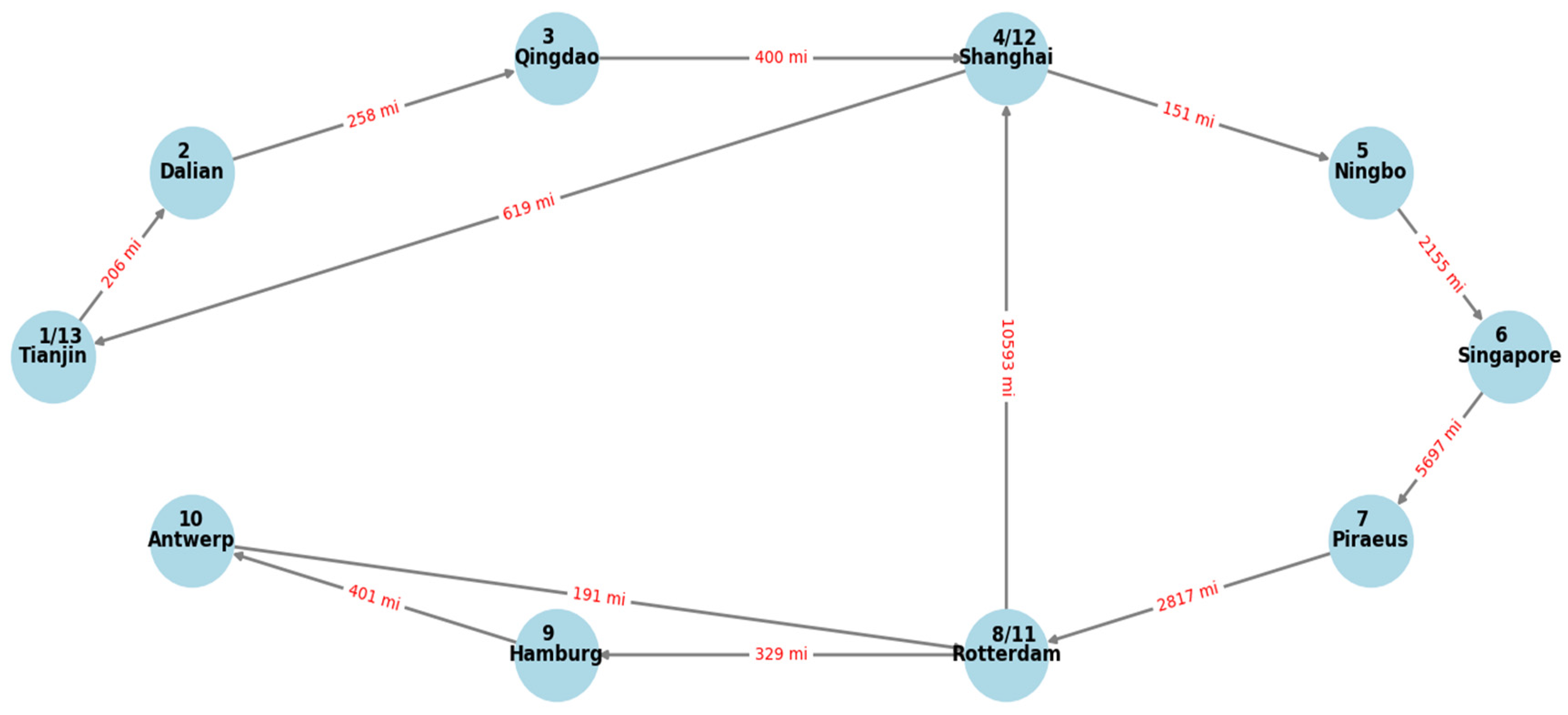
The China–Europe route, a key maritime trade route and an important part of China’s Belt and Road Initiative, starts and ends in Tianjin. As shown in Figure 1, Route 1 starts in Tianjin and proceeds to Dalian (206 miles), Qingdao (258 miles), Shanghai (400 miles), Ningbo (151 miles), and Singapore (2155 miles). It then continues to Piraeus, Greece (5697 miles), Rotterdam (2817 miles), Hamburg (329 miles), and Antwerp (401 miles). The route returns to Rotterdam (191 miles), Shanghai (10,593 miles), and finally back to Tianjin (619 miles).

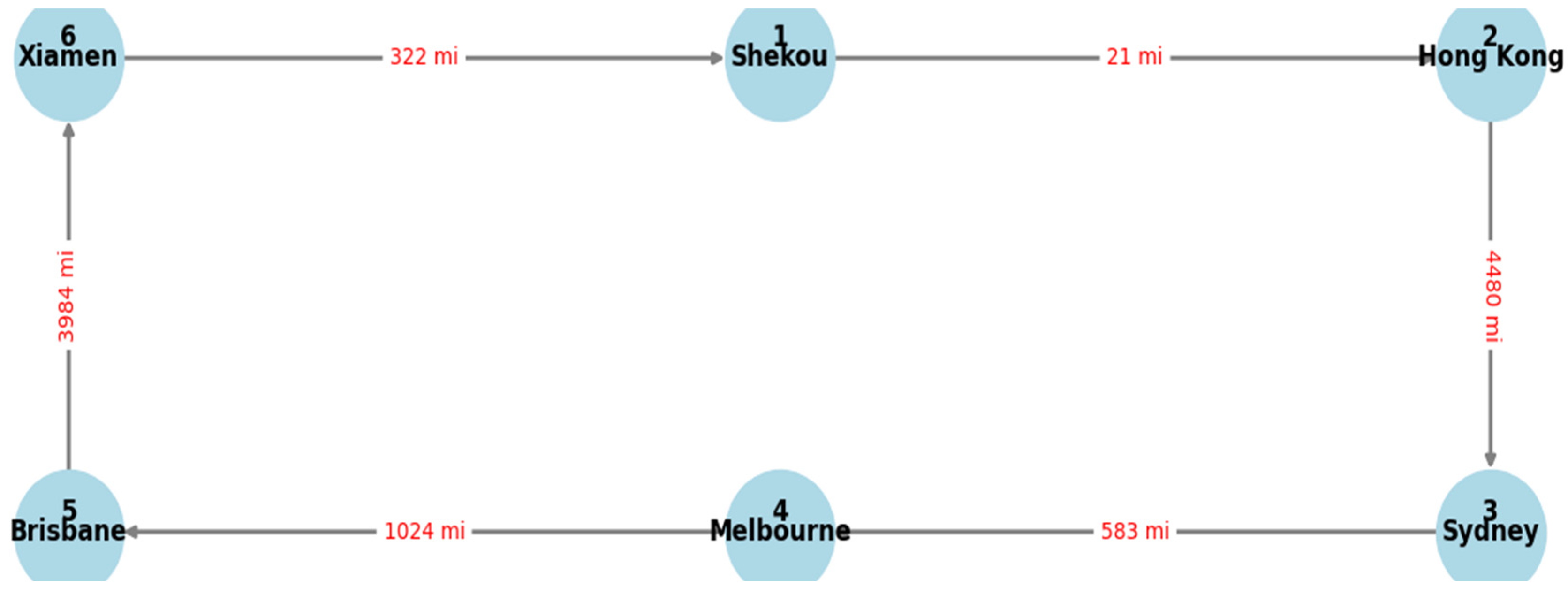
The China–Australia route (Route 2) is a direct service, originating at Xiamen Port, and offers the fastest container shipping link from South China to Australia. The complete port mileage chart for this route is presented in Figure 2. The vessels depart from Xiamen Port, traveling to Shekou (322 miles), then to Hong Kong (21 miles), followed by Sydney (4480 miles), Melbourne (583 miles), and Brisbane (1024 miles), before finally returning to Xiamen Port (3984 miles).

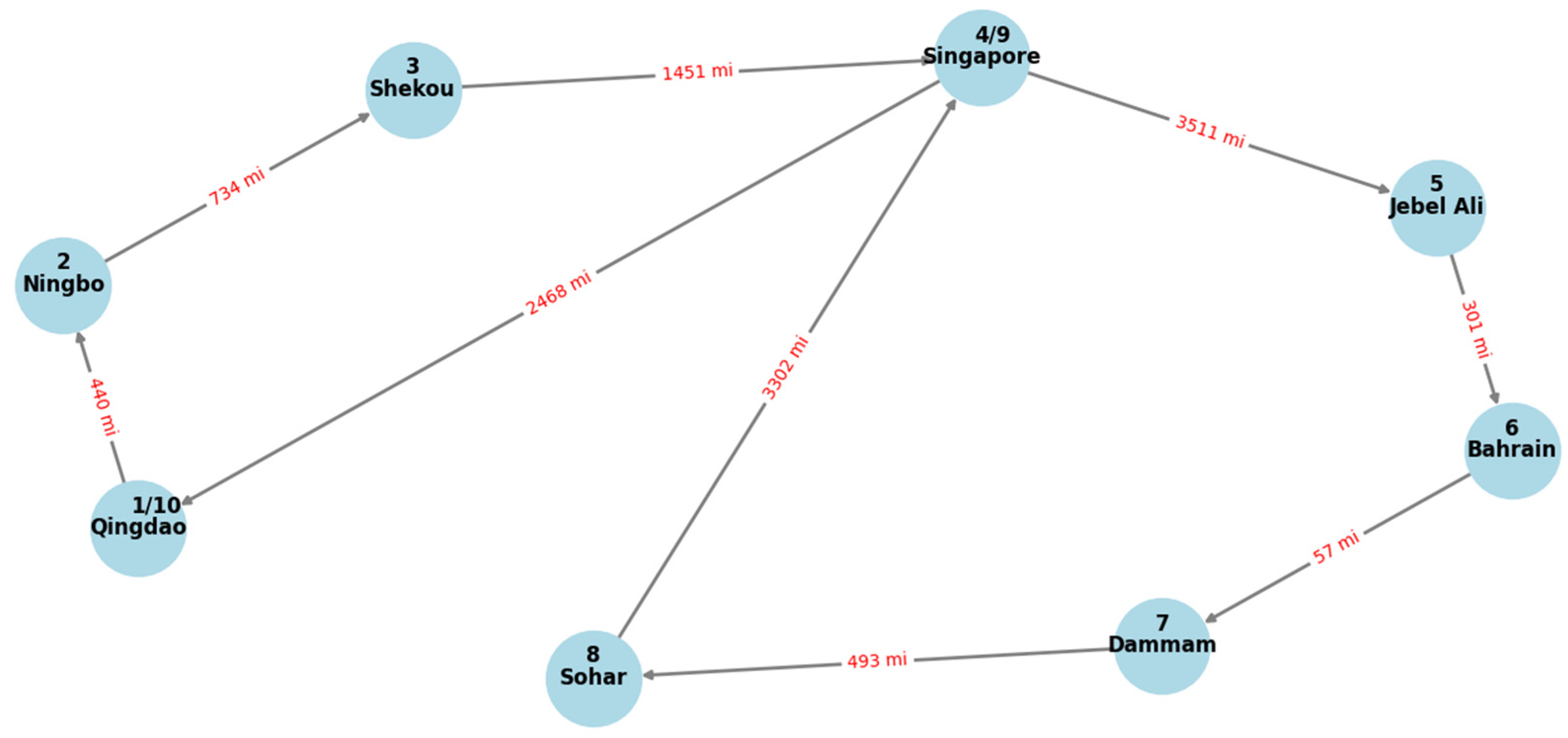
Route 3, as shown in Figure 3, Company Z’s Far East to Middle East route, begins at Qingdao Port, traveling to Ningbo (440 miles), Shekou (734 miles), and Singapore (1451 miles). From Singapore, the vessels continue to Jebel Ali (3511 miles), Bahrain (301 miles), and Dammam (57 miles), before reaching Sohar (493 miles). After Sohar, the ships return to Singapore (3302 miles) and, ultimately, back to Qingdao (2468 miles). The basic details of Company Z’s routes and ships in Routes 1, 2, and 3 are provided in

Table 1. The basic information of routes and ships in routes 1, 2, and 3 of Company Z.

	Route 1	Route 2	Route 3
Route mileage (mile)	23,818	10,424	12,757
Flight time (hours)	2072	1049	1153
Departure interval (days)	7	7	7
Number of ships assigned to the route	13	7	7
Main ship types (TEU)	19,150	5250	13,386
Average speed (kn/hour)	16	13	15
In port time (hours)	558	232	288
Sailing time (hours)	1514	817	865
Cost of newbuilding ships (USD million)	180	87	145
Salvage value of ships (USD million)	38	17.25	27.25
Ship age (Years)	5	21	9
The power of main engine (KW)	95,072	42,950	72,240
The power of auxiliary engine (KW)	8200	4700	7944
Forward displacement (Ton)	157,344	39,318.6	122,932.8
Reverse displacement (Ton)	118,008	52,424.8	92,199.6
Forward freight (USD)	722	190	879
Reverse freight (USD)	433	114	527

.

4.2. Container Ship Freight

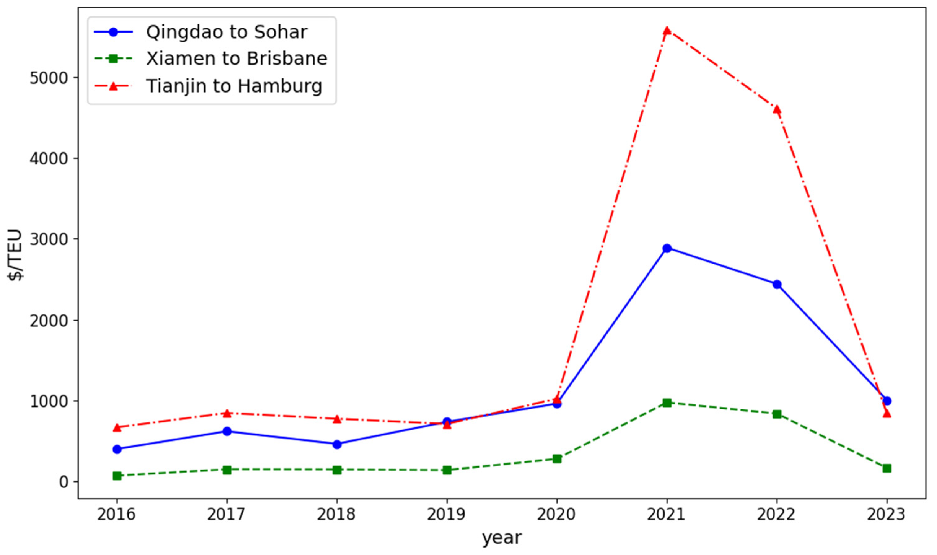
In fact, 2023 is the third year after the implementation of the new IMO 2020 regulations and the first year that carbon reductions come into effect precisely. Due to economic globalization and stable demand growth in China and emerging markets, the container liner shipping market is relatively stable, and the freight rates of the three routes had less fluctuation before the epidemic. There was a small increase in container freight rates from 2019 to 2020 due to the implementation of the emission reduction policy, and the increase in the price of low-sulfur bunker fuels for ships, driven by the new regulations, exacerbated the cost of shipping leading to a small increase in freight rates. In late 2020, affected by the new crown epidemic, the international supply chain was broken, the container liner faced a situation that it is hard to categorize, and the container liner freight rate skyrocketed, especially as the freight rate of the China–Europe container liner route was 5–6 times of the previous years. Influenced by Chinese domestic epidemic prevention and control policies as well as global supply chain shifts, container liner freight rates on the three routes weakened sharply in the second half of 2021 from previous abnormal highs and continued to slow down in early 2022, returning to the pre-2020 range of freight rate movements, as shown in Figure 4.

Through the research information on Clarkson Intelligence Network, the container liner freight rates in the case study of this paper adopted the 2023 freight rates of container liner routes as the benchmark for research and analysis. The price of the China–Europe liner route from Tianjin to Hamburg was 722 USD/TEU, the reverse freight rate was 433 USD/TEU, and the reverse freight rate was 60% of the forward freight rate. The forward freight rate from Xiamen to Brisbane in the Asia–Pacific route is 190 USD/TEU, and the reverse freight rate was calculated by using the reverse freight rate of the China–Europe route, which was 114 USD/TEU; the freight rate from Qingdao to Sohar was 879 USD/TEU; and the reverse freight rate was 527 USD/TEU for the case study. For the freight capacity of the ship, in this case study, the forward capacity was 80% of the ship’s rated capacity and the reverse capacity was 60% of the rated capacity.

4.3. Model Solution Analysis

We conducted a cost–benefit analysis of different fuel replacement options for different routes, shown in what follows.

4.3.1. Cost–Benefit Analysis of Low-Carbon Fuels for Route 1

According to the information provided on Company Z’s website, there are currently 13 container vessels deployed on the baseline case study routes and a weekly frequency of container liner departures is maintained, with the average speed on the routes maintained at 16 knots.

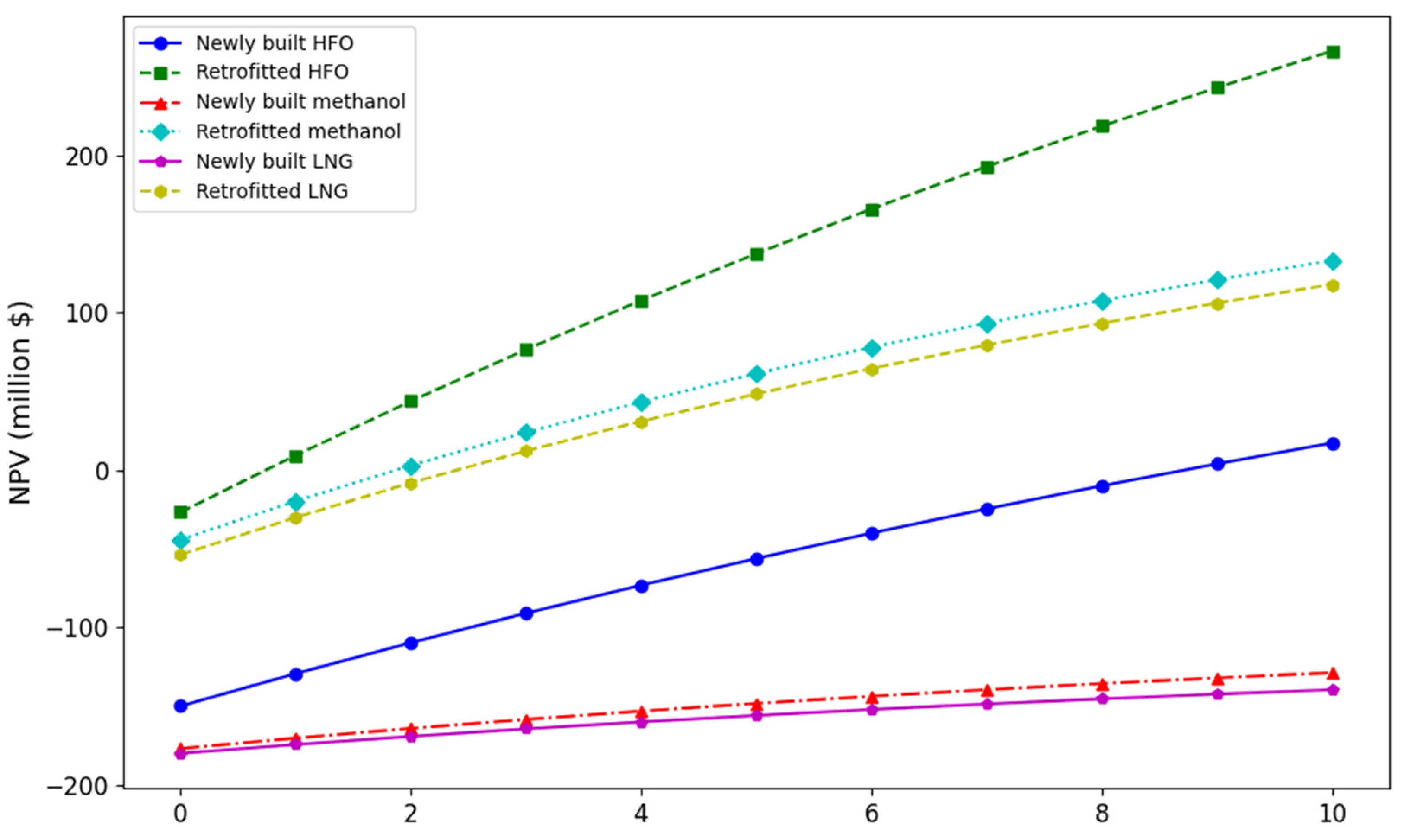
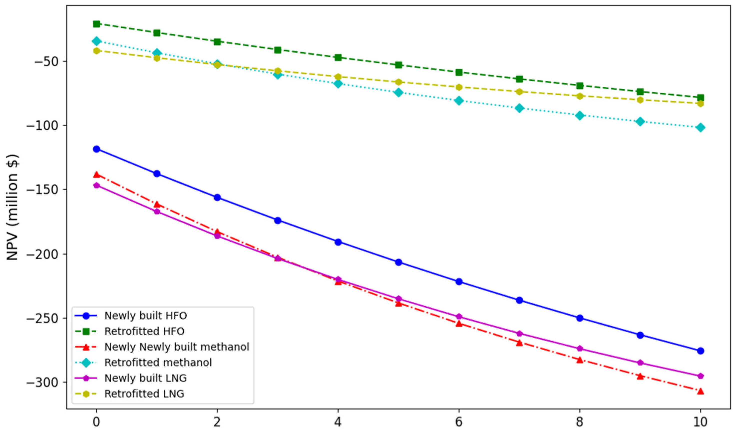
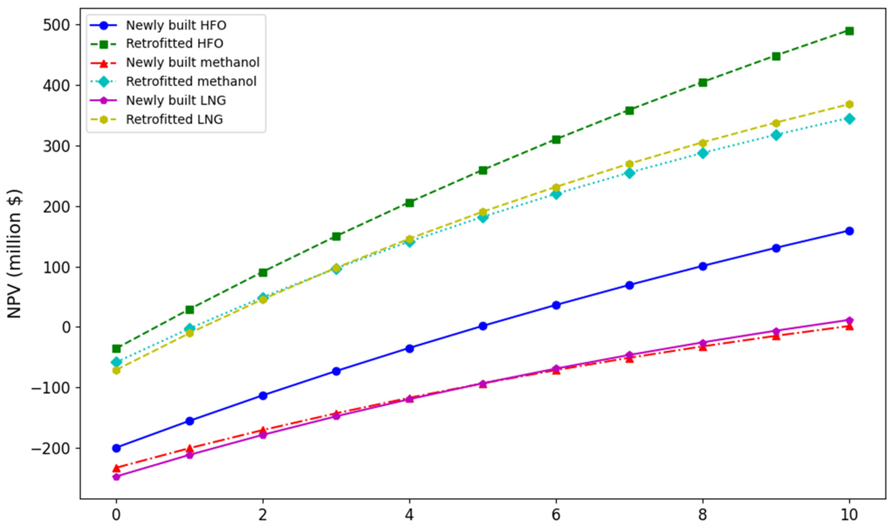
Figure 5 and Figure 6 show the NPVs of using HFO fuel and low-carbon fuels (methanol fuel and LNG fuel) in Route 1 over the next 10 years under the current shipping market line, respectively. As a result of the current global economic downturn, the shipping market is weak and both bunker prices and container freight rates are running at historically low levels. In Route 1, under benchmark conditions, the feasible scenarios for the use of replacement fuels during the study period are newly built HFO and retrofitted HFO, and retrofitted methanol and retrofitted LNG.

The highest NPV among the various scenarios is the retrofitted HFO, which has the advantages of a short payback and short retrofit cycle. The payback period for the retrofitted LNG is 3 years and the payback period for the retrofitted methanol is 2 years. The payback period for the newly built HFO is 9 years. The NPVs for the newly built methanol and LNG are negative over the study period.

The NPV at the end of the study period is 12.9% higher for the retrofitted methanol compared to that of the retrofitted LNG option for large container ships. The NPV of the newly built methanol is 7.8% higher than that of the newly built LNG. While the fuel prices for LNG and methanol fall and container freight rates increase, the options for newly built LNG and newly built methanol may be a more viable to investment for the carbon reduction programs of Route 1.

4.3.2. Cost–Benefit Analysis of Zero-Carbon Fuels for Route 1

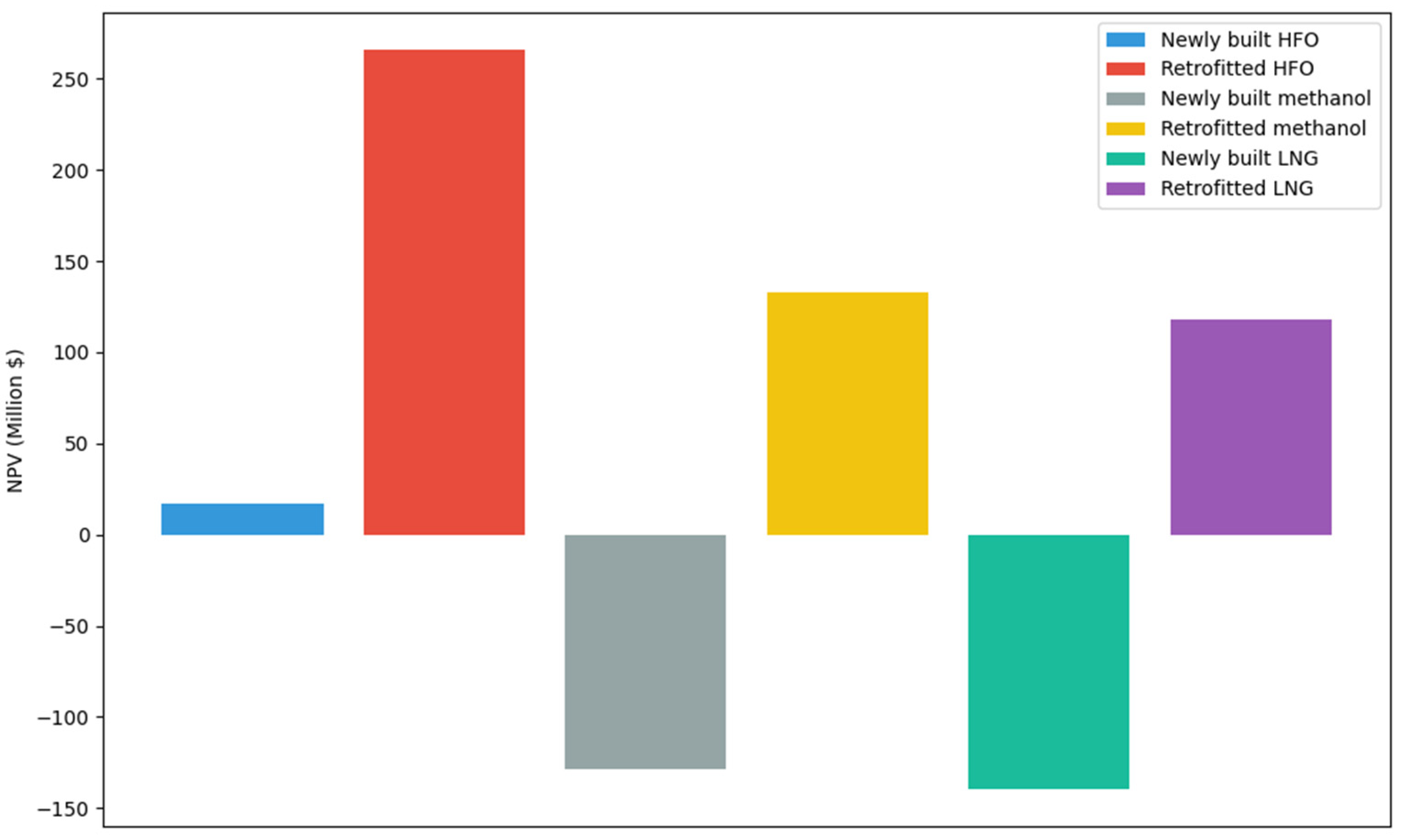
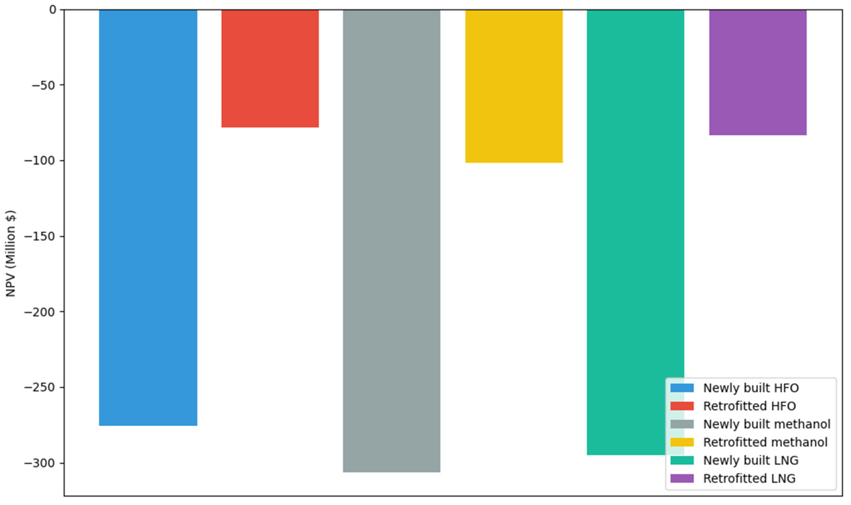
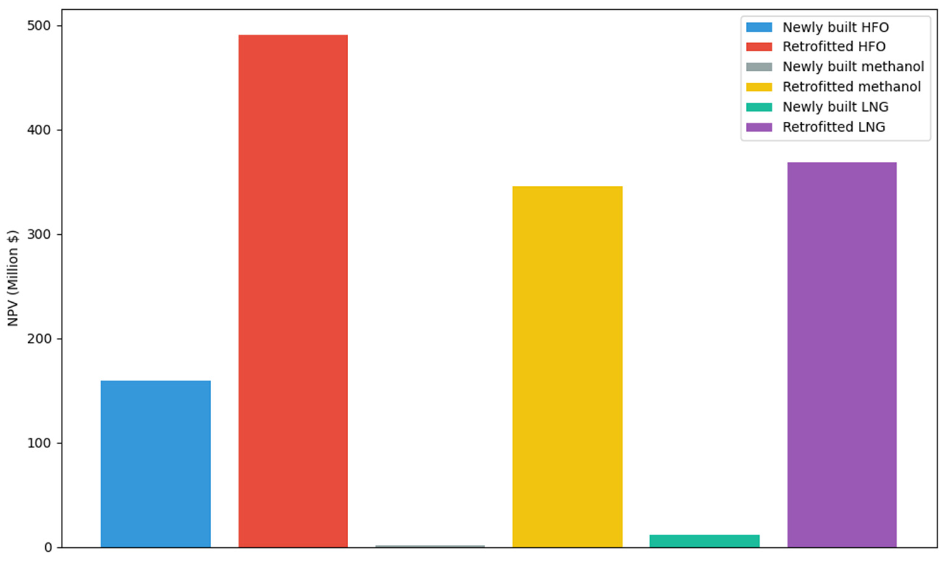
In Figure 7 and Figure 8, we can observe that the option of retrofitted ammonia fuel has the best NPV of the zero-carbon fuels at the end of the study period. The newly built ammonia scenario ships have an NPV of less than 0 over the study period and is not investment-feasible.

The carbon abatement scenarios of newly built hydrogen and retrofitted hydrogen had investment returns of less than 0. The retrofitted hydrogen scenario was 52.1% higher than the newly built hydrogen scenario, but the annual return of less than 0 did not have an investment value in the study period.

The payback period of the retrofitted ammonia option is 3 years, which is characterized by a short payback period and high investment feasibility. The investment return of the newly ammonia and hydrogen under the baseline conditions was negative and had no investment value. To summarize, for a future investment decision of container ship capacity renewal, the option of retrofitted ammonia has the best investment feasibility for zero-carbon fuels in Route 1.

4.3.3. Cost–Benefit Analysis of Low-Carbon Fuels for Route 2

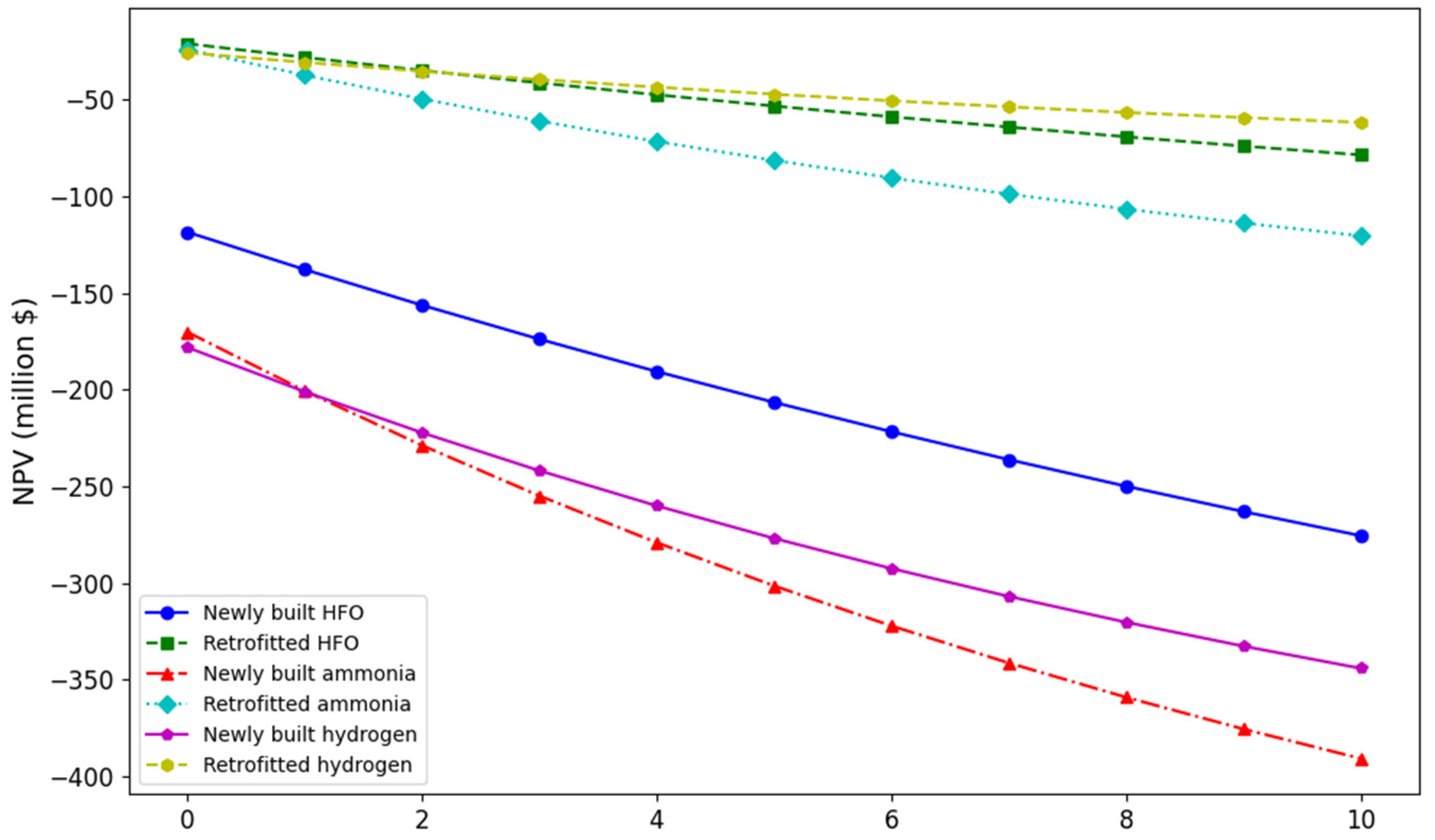
According to the information provided on the website of Company Z, there are currently seven container ship vessels deployed in Route 2, and the weekly departure frequency of container liners is maintained, with the average speed on the route maintained at 12.8 knots.

A cost–benefit analysis of the carbon reduction options for the main vessel types in Route 2 was conducted under baseline conditions, as shown in Figure 9 and Figure 10. When using the low-carbon fuel (LNG fuel and methanol fuel) scenarios, under the baseline conditions, the NPVs of the scenarios using low-carbon fuel and the HFO fuel scenarios were lower than zero and did not have an investment value over the study period due to the excessively low price of the freight rates and the negative return on investment.

The scenario using newly built methanol ships has the smallest return on investment, and the NPV of the scenario using retrofitted LNG ships is 18% higher than the NPV of the methanol fuel scenario. The annual net return is 11.7% higher for the newly built LNG than for the newly built methanol option, and 57.2% higher for the retrofitted LNG than the retrofitted methanol option. In summary, for low-carbon scenario, the carbon reduction option of retrofitted LNG is suggested to be used in Route 2.

4.3.4. Cost–Benefit Analysis of Zero-Carbon Fuels for Route 2

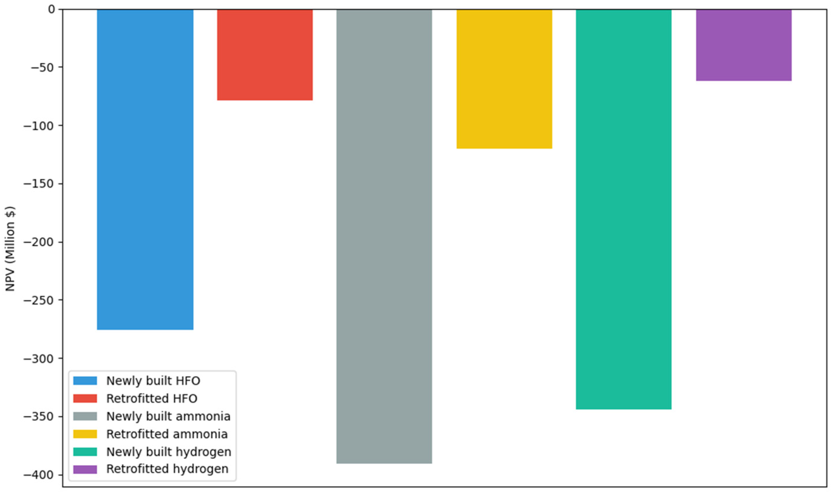
As shown in Figure 11 and Figure 12, under the baseline conditions, the investment return of the emission reduction program using zero-carbon fuels for the existing container ships is negative and not investment-feasible. For small ships in Route 2, the NPV of retrofitted hydrogen was 48.7% higher than that of retrofitted ammonia, and the NPV of newly built hydrogen is 11.9% higher than that of newly built ammonia under the baseline conditions when using this ship type in implementing the carbon emission reduction policy.

The annual net return from retrofitted hydrogen is 62.6% higher than that from retrofitted ammonia, and the annual net return from newly built hydrogen is 24.7% higher than that from newly built ammonia. The annual net benefit of retrofitted hydrogen is 62.6% higher than that of retrofitted ammonia, and that of newly built hydrogen is 24.7% higher than that of newly built ammonia ships.

To sum up, the carbon emission reduction plan of using zero-carbon fuel for small ships does not have investment feasibility under the baseline conditions. Shipowners can consider optimizing the operation of the routes on the basis of using HFO fuel to improve the voyage revenue of the routes before analyzing the investment decision of using replacement fuels for ships for carbon emission reductions.

4.3.5. Cost–Benefit Analysis of Low-Carbon Fuels for Route 3

According to the information provided on Company Z’s website, there are currently seven container vessels deployed in Route 3, and the weekly departure frequency of container liners is maintained, with the average speed on the route maintained at 14.8 knots.

As shown in Figure 13 and Figure 14, under the baseline conditions, through the cost–benefit analysis of the carbon emission reduction program using replacement fuels for the main ship types in Route 3, the carbon emission reduction investment program of using low-carbon fuels for ships has an NPV of >0 for newly built and retrofitted ships during the study period, which makes it a feasible investment.

The carbon abatement investment scenario using retrofitted LNG has the best NPV, followed by retrofitted methanol ships. The payback period for newly built LNG and methanol is 10 years, and the annual investment return of the newly built LNG is 6.37 times higher than that of the newly built methanol.

Under baseline conditions, the NPV of the newly built LNG at the end of the study period is 6.8 times higher than that of the newly built methanol. The payback period for retrofitted LNG and methanol ships is 2 years, and the scenarios that use retrofitting have the advantages of a shorter payback period and a higher return on investment.

The difference in NPVs between retrofitted LNG and retrofitted methanol was not significant. The NPV of using the retrofitted LNG scenario is 6.5% higher than that of the retrofitted methanol scenario, and the annual investment return is 8.7% higher during the study period. The best low-carbon fuel abatement option in Route 3 was the retrofitted LNG, which has the best investment feasibility and return on investment.

4.3.6. Cost–Benefit Analysis of Zero-Carbon Fuels for Route 3

In Figure 15 and Figure 16, we can observe that, among the NPVs of abatement scenarios using zero-carbon fuels for large ships, the retrofitted methanol has the best NPV over the study period. The newly built ammonia has an NPV of less than 0 over the study period and is not investment-feasible.

Under the baseline conditions, the annual investment return of the retrofitted HFO is 32.7% higher than that of the retrofitted ammonia during the study period. The NPV of the retrofitted HFO is 61.3% higher than that of the retrofitted ammonia at the end of the study period. The payback period of the retrofitted ammonia scenario is 3 years, which is characterized by a short payback period and higher investment feasibility. The payback period of the newly built hydrogen is 11 years, which does not have investment value in the study period, but has some investment feasibility under the uncertain future shipping market. The investment returns of the newly built ammonia and newly built hydrogen under the baseline conditions are negative and do not have investment value.

In summary, the retrofitted ammonia is the best investment feasibility option for zero-carbon fuels on container ship capacity renewal in Route 3.

5. Conclusions

In this paper, a cost–benefit analysis model is proposed to conduct quantitative comparative analyses for replacement fuel ships from the perspective of the shipowners, with low-carbon fuel ships (LNG-fueled and methanol-fueled) and zero-carbon fuel ships (ammonia-fueled and hydrogen-fueled) as feasible options for shipowners.

Under the baseline conditions, using the cost–benefit analysis, it can be seen that there are three scenarios that satisfy the investment feasibility in Route 1: the NPVs at the end of the study period are the retrofitted methanol, retrofitted LNG, and retrofitted ammonia ship scenarios, in descending order of magnitude.

In Route 2, there are zero scenarios that satisfy the investment feasibility, and the NPVs at the end of the study period are, in descending order, the retrofitted hydrogen, retrofitted LNG, and retrofitted methanol ship scenarios.

There are five scenarios that satisfy investment feasibility in Route 3, and the end-of-study NPVs are, in descending order, the retrofitted LNG, retrofitted methanol, retrofitted ammonia, newly built LNG, and newly built methanol scenarios.

In summary, the retrofitted LNG ships is prioritized in Route 1, retrofitted hydrogen in Route 2, and retrofitted methanol in Route 3. This may be attributed to the advantages of using the retrofitted option with a better return on investment, low initial investment costs, and a short retrofit cycle.

Our study employed an optimization model that, while robust in its theoretical framework, relies on predefined parameters and constraints. These parameters are based on current technological, economic, and regulatory environmental factors, which may evolve over time. Consequently, the model’s applicability might be limited under different future conditions.

To make the problem tractable, we made several simplifications and assumptions regarding the operating conditions, cost calculations, and technology performance. While these assumptions are justified within the context of our model, they do limit the generalizability of our results to real-world scenarios that may not align perfectly with these assumptions.

The accuracy of the results is highly dependent on the quality and granularity of the data used. In areas where data were limited or assumptions had to be made, the precision of the outcomes could have been affected.

Our model primarily addresses economic and technological aspects of optimization. It does not fully integrate potential environmental and social impacts, which are critical for a holistic assessment of sustainability practices.

This study laid a foundational analysis focusing on the shipowners’ response to carbon emission reduction initiatives under baseline conditions. We considered key influencing factors, such as sailing distances, fuel prices, and container freight rates, which play a significant role in shaping shipowner decisions. However, the complexities of maritime operations and the diverse challenges faced by shipowners require a broader scope of analysis to fully capture the dynamics at play.

Future research should aim to incorporate additional influencing factors that affect shipowner operations and decision-making. This includes, but is not limited to, the following:

(1)

Environmental regulations: More in-depth analysis of local and international regulations that impact operational costs and strategic decision-making. This involves not just current regulations but also potential future legislative changes that could alter operational paradigms.

(2)

Technological advancements: The impact of emerging technologies, such as digitalization, advanced materials for shipbuilding, and alternative propulsion systems that could significantly influence fuel efficiency and carbon emissions.

(3)

Economic factors: Broader economic indicators that influence shipping demand and supply, such as global trade volumes, economic cycles, and geopolitical tensions that might affect shipping routes and freight rates.

(4)

Social and environmental concerns: Increasing awareness and advocacy towards environmental and social issues could alter consumer and corporate behaviors, influencing the routes chosen, speeds maintained, and investments made in greener technologies.

(5)

Market competition: The strategies adopted by competitors, including alliances and mergers, can also significantly influence individual shipowners’ operational and strategic decisions.