Impact of Road Gradient on Fuel Consumption of Light-Duty Diesel Vehicles

Abstract

The geometric alignment of highways directly affects the fuel consumption of motor vehicles. To analyze the impact of the road gradient on fuel consumption, actual road tests were conducted in plateau and mountainous areas. Geographic Information Systems (GISs) were used to calculate road gradients, and Vehicle Specific Power (VSP) distributions were obtained through testing, serving as inputs for the motor vehicle emission simulator (MOVES) model. Finally, the simulation results were verified against the experimental results. The findings indicate a strong positive correlation between road gradients ranging from −5% to +5%, the VSP, and fuel consumption. At a constant gradient, the fuel consumption rate increases with the vehicle speed; the fuel consumption factor is lowest at 60 km/h and highest at 40 km/h. Under both constant and actual driving speeds, when the absolute values of uphill and downhill gradients are the same, the average fuel consumption for both uphill and downhill driving shows that, at gradients of 1% to 3%, the fuel savings from downhill driving can offset the additional fuel consumption on uphill driving. At gradients of 4% to 6%, the increase in fuel consumption on uphill driving surpasses the savings from downhill driving. During uphill climbs, lower speeds within the mid-to-low range result in lower fuel consumption and greater reserve power. The MOVES model demonstrates good adaptability in plateau and mountainous areas.

1. Introduction

Approximately 26% of China’s territory is located above 1000 m in altitude, and there are over 15 million motor vehicles in high-altitude areas [1]. Nearly two-thirds of China’s land area is mountainous, with Yunnan Province in particular having 84% of its territory covered by mountains, forming a unique plateau and mountainous geographical conditions. The roads in the plateau and mountainous areas feature significant altitude differences and notable changes in road gradients. Driving on slopes increases the power demand of motor vehicles, leading to higher fuel consumption. This poses issues related to energy consumption, emissions, and safety while driving in mountainous areas, which have garnered widespread attention [2,3,4,5].

To analyze the impact of road gradient on fuel consumption, Faria et al. [6] established a real driving database by observing 47 drivers over six months and found that aggressive driving has varying effects on fuel consumption across different road gradients. On low-gradient roads, aggressive driving can increase fuel consumption by up to 250%. Wu et al. [7] developed a Real-World Fuel Consumption Rate (RFCR) model using samples from 201 car brands and 34 cities, discovering that temperature and altitude significantly affect fuel consumption. Boriboonsomsin et al. [8] found that when road gradients are too steep, vehicles require more power, leading to increased fuel consumption. Compared to flat roads, fuel economy improves nearly twofold on downhill routes but decreases by 1.5 to 2 times on uphill routes. Frey et al. [9] showed in Real Driving Emission (RDE) experiments that neglecting uphill gradients can underestimate the vehicle fuel consumption and emissions by 16–22%, while neglecting downhill gradients can overestimate them by 22–24%. Liu et al. [10] demonstrated that when road gradients increase from 0.5% to 6%, the fuel consumption rises by approximately 140%.

Due to the ability of microscopic fuel consumption models to instantaneously relate vehicle parameters, driving conditions, road types, and other factors to fuel consumption, they have garnered significant attention from scholars [11,12]. Models such as MOVES, IVE, and CMEM for estimating fuel consumption have become current research hotspots. Fuel consumption calculation models based on the Vehicle Specific Power (VSP) distribution have the advantage of easier access to VSP data. The United States Environmental Protection Agency (EPA) has developed the MOVES model, a VSP-based fuel consumption and emission prediction model, which calculates the total fuel consumption of a vehicle during its operation by summing the fuel consumption across different driving condition intervals [13].

In summary, the primary objective of this study was to investigate the impact of the road gradient on the fuel consumption for light-duty diesel vehicles in plateau and mountainous areas, where obtaining accurate road gradient data is challenging. Due to this difficulty, previous analyses of the impact of road gradient on fuel consumption have been relatively coarse, and fuel consumption models have seldom been applied in these regions while considering the road gradient.

To address this gap, we conducted actual road driving tests on plateau and mountainous roads. Utilizing GIS technology, we accurately calculated the road gradient for each test segment. This enabled us to collect detailed data on the road gradient, VSP, and instantaneous fuel consumption on a second-by-second basis.

Our main goals were to analyze the relationship between the road gradient, VSP, and fuel consumption, and to verify these findings using the MOVES model. Furthermore, we aimed to assess the adaptability of the MOVES model for light-duty diesel vehicles in plateaus and mountainous areas, considering the unique challenges posed by these environments, such as varying altitudes, complex terrains, and extreme weather conditions.

2. Materials and Methods

2.1. Testing Equipment

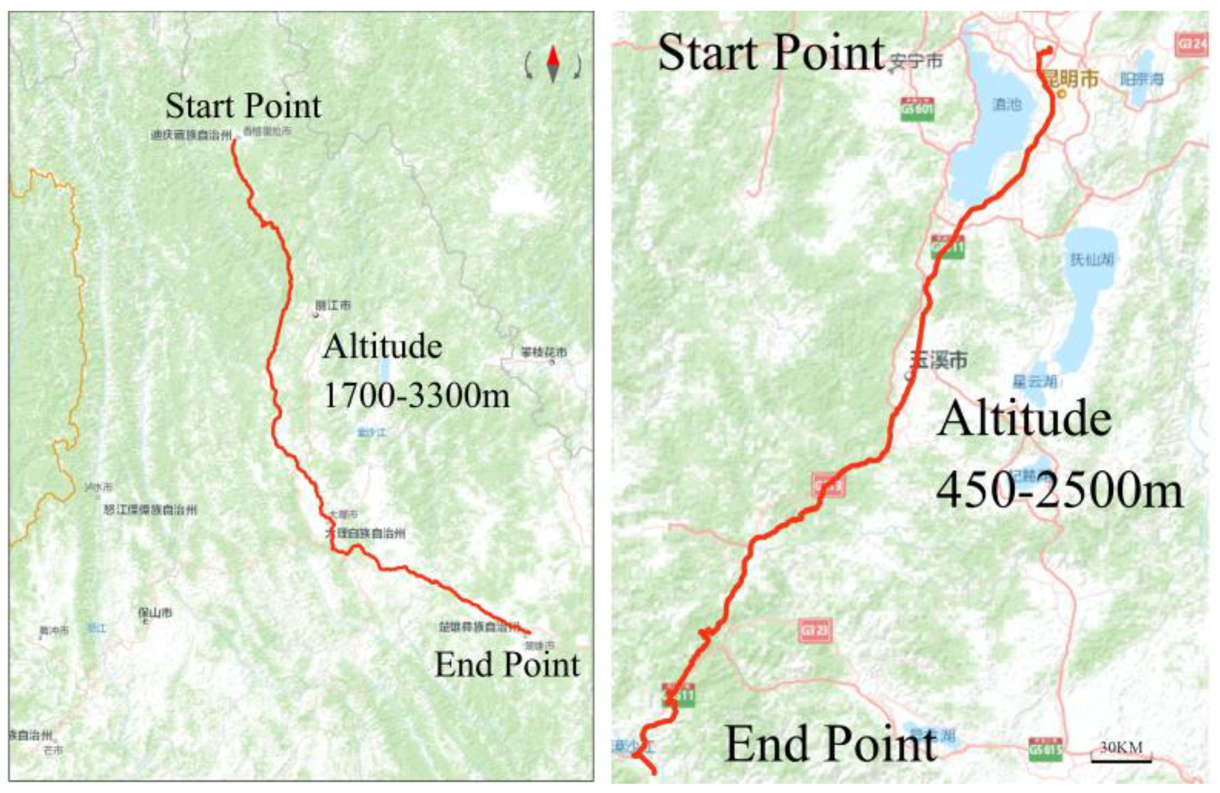
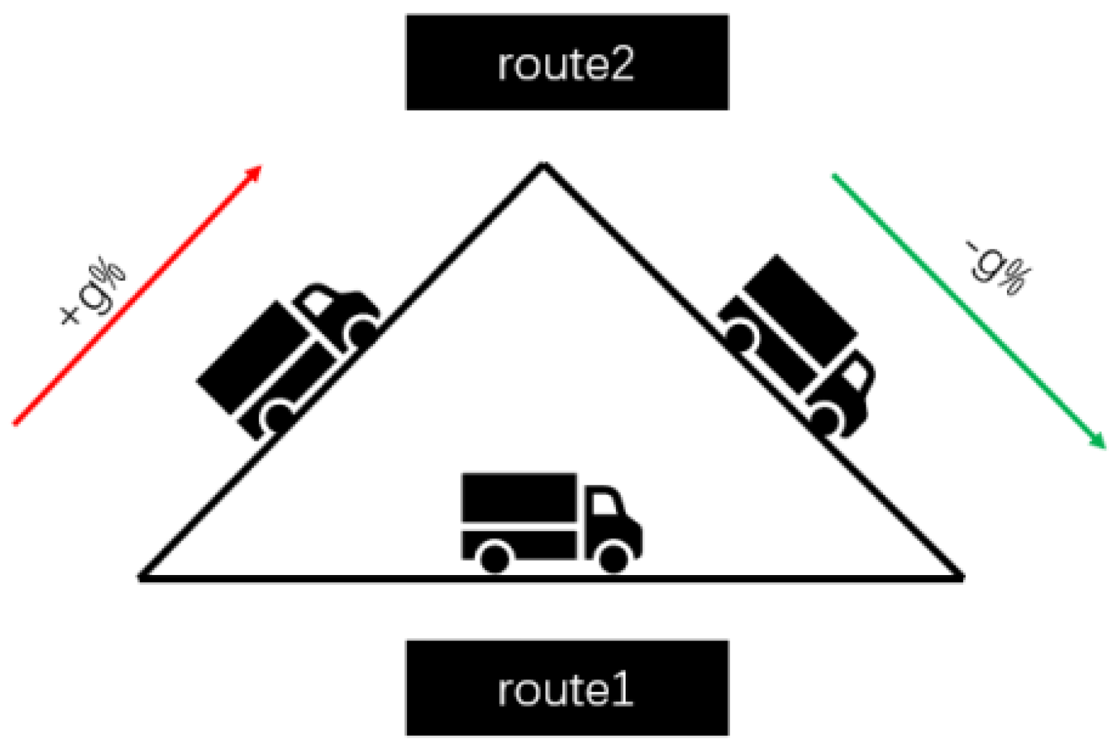
The test vehicle utilizes a Foton light truck, equipped with a diesel engine manufactured by Kunming Yunnei Power. The test vehicle is in good condition, and its main parameters are shown in

Table 1. Main engine parameters of the test vehicle.

Type	Four-Stroke Diesel Engine
Compression ratio	16.8:1
Engine displacement/L	3.76
Cylinder bore × stroke/mm	102 × 115
Rated power(rpm)/KW(r·min−1)	95 (3000)
Maximum torque (rpm)/N·m(r·min−1)	365 (1600)
Idle speed/r·min−1	800 ± 30
Fuel supply system type	High-Pressure Common Rail

. Vehicle movement data and fuel consumption information were collected using GARMIN GPS and VBOX, respectively.

2.2. Testing Route

On plateau and mountainous roads, actual vehicle experiments were conducted to collect vehicle movement data. The test road segments were selected on the representative highways of Kunming to Yuanjiang (with an altitude range of 450–2500 m) and Shangri-La to Chuxiong (with an altitude range of 1700–3300 m) in the Yunnan plateau and mountainous region. These two segments exhibit significant variations in altitude and road gradients. A total of 66,000 data points were collected, and the routes are illustrated in Figure 1.

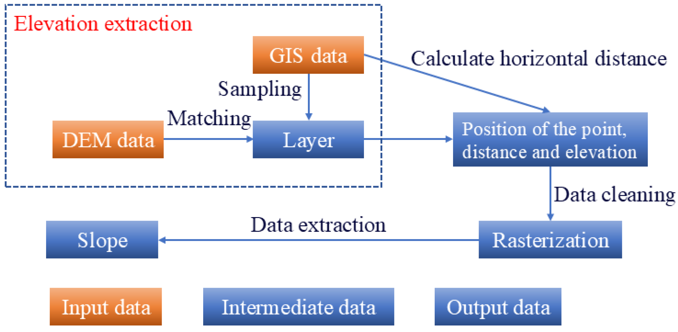
2.3. Gradient Calculation

The road gradient was analyzed using GIS based on Global Positioning System (GPS) data. The latitude and longitude data collected by GPS were imported into GIS software (ArcGIS 10) to generate a point layer along the centerline of the road in the geographic information system. The Digital Elevation Model (DEM) was connected to the point layer, and elevation was added to each point. Incorrect elevation data were removed, and finally, statistical tools were used to extract the gradient of each point [14]. This allowed for real-time analysis of the impact of road gradient on transient vehicle emissions. Wang Xuming analyzed the method of measuring road gradient based on GPS, and the experimental results showed that the error between the road gradient measured by the GPS method and the standard ramp measurement was within 5%, which could meet the actual needs [15]. The flowchart for extracting the gradient is shown in Figure 2.

3. Results and Discussion

The gradient not only increases the load on the engine, but also affects the vehicle’s motion state, so the impact of the gradient on fuel consumption cannot be analyzed in isolation. The VSP integrates both the gradient and vehicle motion state, allowing for a more comprehensive analysis of the gradient’s influence on fuel consumption. We will analyze the correlation between the VSP and fuel consumption in plateau and mountainous regions, and then use the MOVES model for verification.

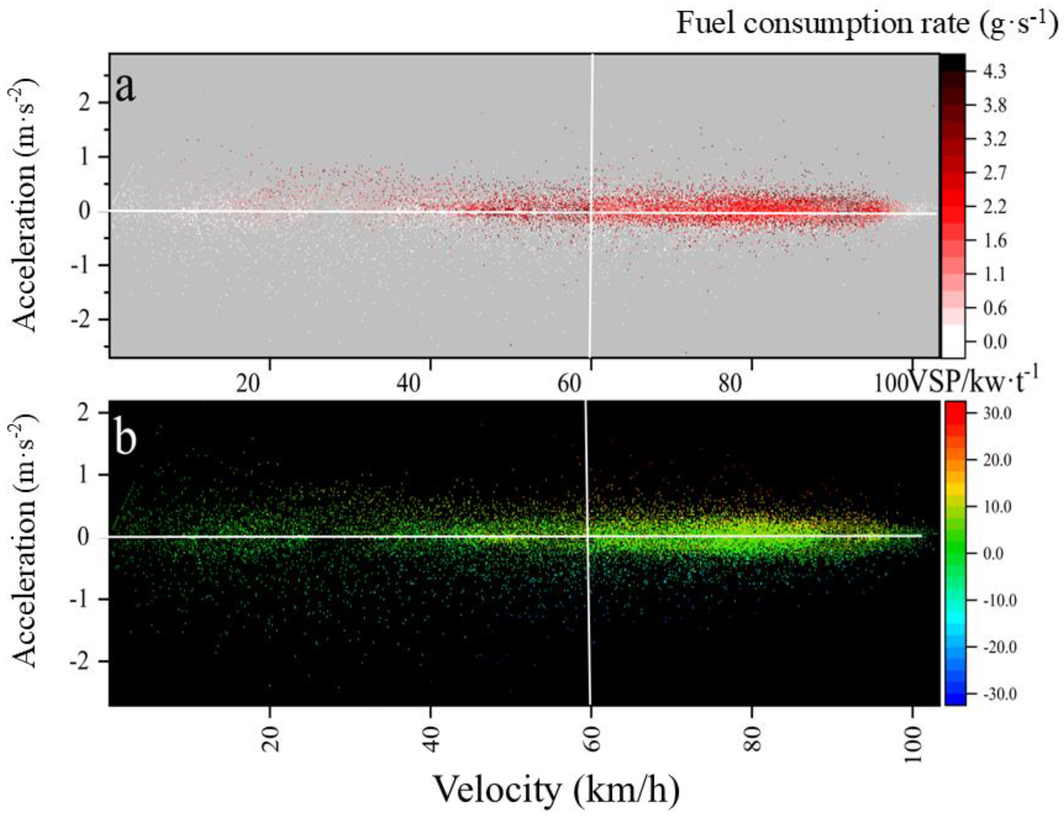
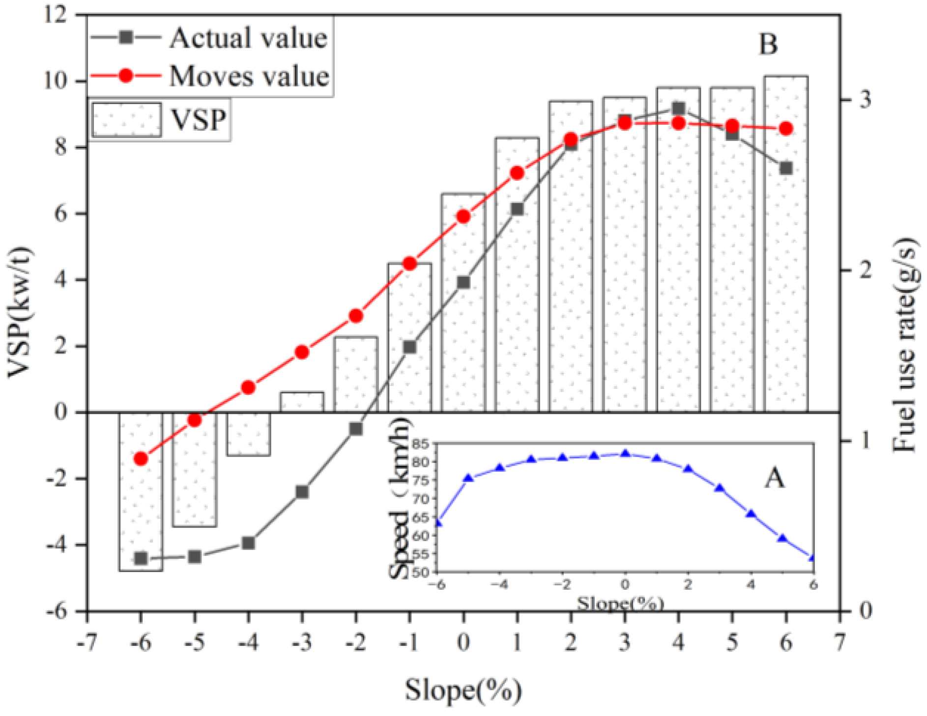
3.1. The Impact of Slope on Vehicle Movement State

Figure 3 illustrates the impact of the gradient on the vehicle’s motion state. As the gradient increases, the absolute values of acceleration and deceleration first increase and then decrease, with a turning point near −1%. Both extreme acceleration and extreme deceleration occur during downhill travel. The larger the absolute value of the gradient, the smoother the changes in acceleration and deceleration. Low vehicle speeds primarily occur during uphill travel, and when the gradient exceeds +3% during uphill, there is a noticeable decrease in the vehicle speed. Overall, the vehicle speeds on the downhill sections are higher than those on the uphill sections. Liu et al. [16] studied the variation in the shape characteristics of the joint distribution of the vehicle speed and acceleration with the road gradient. Their results showed that, under natural traffic flow conditions, as the gradient increases from −3% to +3%, the curves of extreme acceleration and average acceleration for all vehicle types exhibit a clear trend of decreasing from large to small. An increase in the gradient significantly reduces both extreme acceleration and average acceleration. The road gradient has a significant impact on the vehicle’s motion state.

The power required for a vehicle’s powertrain system to overcome the resistance to forward motion while achieving the desired speed and acceleration is known as the VSP. Jiménez-Palacios [17] proposed a calculation formula suitable for Vehicle Specific Power, which is

VSP = v × [1.1 a + 9.8 s + 0.132] + 0.000302 v³

(1)

VSP stands for Vehicle Specific Power, measured in kw/t; v represents the vehicle’s traveling speed, measured in m/s; a represents the instantaneous acceleration of the vehicle, measured in m/s²; and s represents the slope, measured in percentage.

Equation (1) elucidates the relationship between the VSP and various factors including the vehicle kinetic energy (speed and acceleration), potential energy (road gradient and speed), rolling resistance work, acceleration resistance work, and aerodynamic drag work. Changes in the gradient lead to alterations in the forces acting on the vehicle, resulting in differences in the vehicle speed and acceleration under different gradient conditions. Consequently, the load on the vehicle’s engine changes, causing corresponding variations in power consumption and fuel consumption.

Figure 4 shows the distribution of the VSP and fuel consumption under different vehicle speeds and accelerations, illustrating that driving styles have a significant impact on fuel consumption. As depicted in Figure 4, the acceleration distribution is mainly concentrated between −0.5 m/s² and 0.5 m/s², indicating a relatively conservative driving style. As the speed increases, accelerations tend to cluster around 0 m/s². High fuel consumption and large VSP values primarily occur at medium-to-high speeds, with peak VSP and peak fuel consumption mainly appearing during large accelerations at high speeds.

Comparing Figure 4a,b, it is observed that the acceleration distribution is relatively dispersed at low speeds. This is attributed to the complex traffic conditions at those speeds, resulting in frequent acceleration and deceleration events. At medium-to-high speeds, the acceleration distribution becomes more concentrated, exhibiting less fluctuation.

To further analyze the relationship between the fuel consumption and VSP, statistical calculations were conducted. The comparison reveals a high correlation between the distribution of fuel consumption and VSP, particularly at medium-to-high speeds. Specifically, the correlation coefficient between the fuel consumption and VSP values at these speeds was calculated and found to be strong, indicating a close relationship between the two variables. These statistical findings support our observation that fuel consumption is highly correlated with the VSP, especially at medium-to-high speeds.

3.2. The Influence of Slope on the Motion State of Vehicles

Figure 5 illustrates the relationship between the road gradient, VSP, and fuel consumption. Changes in the road gradient lead to variations in vehicle motion, which in turn affect the engine power and fuel consumption. Figure 5a shows the impact of the road gradient on the VSP. Within a gradient range of −5% to +5%, the VSP increases in a parabolic manner from −7 kw/t to 12 kw/t as the gradient increases. Figure 5c depicts the effect of the road gradient on the fuel consumption. Within the same gradient range, the fuel consumption exhibits a linear increase trend with increasing gradient. During downhill driving, when the gradient exceeds −4%, the fuel consumption approaches zero. By comparing figures a and c, it can be observed that both the VSP and fuel consumption are close to zero at a gradient of −4%. The peak values of the VSP and fuel consumption occur near a gradient of +4%, and both decrease as the gradient further increases.

Figure 5b displays the relationship between the VSP and fuel consumption. When the VSP ranges from −7 kw/t to 12 kw/t, there is a general inverse parabolic trend between the VSP and fuel consumption. As the VSP increases, the fuel consumption rises slowly. The highest fuel consumption occurs when the VSP equals 10 kw/t. Corresponding to the gradient of +4% in Figure 5a, the fuel consumption is also at its peak in Figure 5c. This is because, under normal conditions, the engine operates at the speed corresponding to its maximum output torque, resulting in optimal fuel economy. However, when the torque is insufficient to overcome the resistance faced by the vehicle, the engine speed decreases, prompting a downshift in gear, a change in transmission ratio, an increase in output torque, and an increase in engine torque, all leading to higher fuel consumption. Figure 5d presents a heatmap of the relationship between the road gradient, VSP, and fuel consumption, showing a strong overall correlation. As both the gradient and VSP increase, the fuel consumption also increases significantly. High fuel consumption is concentrated mainly in the regions of medium-to-high gradients and high VSP values. At a gradient of +4%, when the VSP reaches its peak, fuel consumption is maximized.

For the same gradient value, the corresponding VSP and fuel consumption values fall within a range, with a difference of less than 10 kw/t for the VSP and less than 1 g/s for fuel consumption. The scatter plot of the specific power versus fuel consumption aligns with the trends observed in Pang Ran’s paper [18]. When the gradient ranges from −5% to +5%, the VSP varies between −7 kw/t and 12 kw/t in Figure 5a, and the fuel consumption ranges between 0 and 4 g/s in Figure 5c. By combining Figure 5a,b, it can be concluded that there is a high correlation between the gradient and both the VSP and fuel consumption. Analyzing all four plots in Figure 5, it is evident that there is a good positive correlation between the gradient, VSP, and fuel consumption.

4. The Influence of Slope on Fuel Consumption

The MOVES model, developed by the United States Environmental Protection Agency, is a mobile source emission model that provides fuel consumption under 23 operating conditions based on vehicle speed and VSP distribution. The VSP distribution frequency of actual test data is used as the input for the MOVES model, and the final results are validated against actual data. This section analyzes the impact of different gradients on the fuel consumption rate and fuel consumption factor under constant speed conditions. Figure 6 illustrates the differences between uphill, downhill, and flat roads by comparing the average total fuel consumption factors (denoted as (fuel (U + D) 1/2 for actual data and MOVES (U + D) 1/2 for MOVES data) for the uphill and downhill sections of Route 2 with the same gradient to those of Route 1.

G represents the gravity acting on the vehicle, θ is the road angle, Cd is the coefficient of drag, A is the frontal area, ua is the vehicle speed, f is the rolling resistance coefficient, δ is the rotational mass factor, and a is the acceleration. When a vehicle travels uphill, the component of the vehicle’s gravity along the slope manifests as gradient resistance, which is Gsinθ. The road resistance during uphill climbing is Gsinθ + Gfcosθ. During downhill travel, the gradient resistance becomes a driving force, and the vehicle only experiences rolling resistance. In this case, the road resistance is Gfcosθ − Gsinθ.

$$\begin{array}{c}\mathrm{Ft}=Ff+Fw+Fi+Fj\\ =\mathrm{Gsin}\mathrm{\theta }+{\displaystyle \frac{C_D\mathrm{A}{u}_a^2}{21.15}}+\mathrm{Gfcos}\mathrm{\theta }+\mathrm{\delta }\mathrm{m}{\displaystyle \frac{du}{dt}}\end{array}$$

(2)

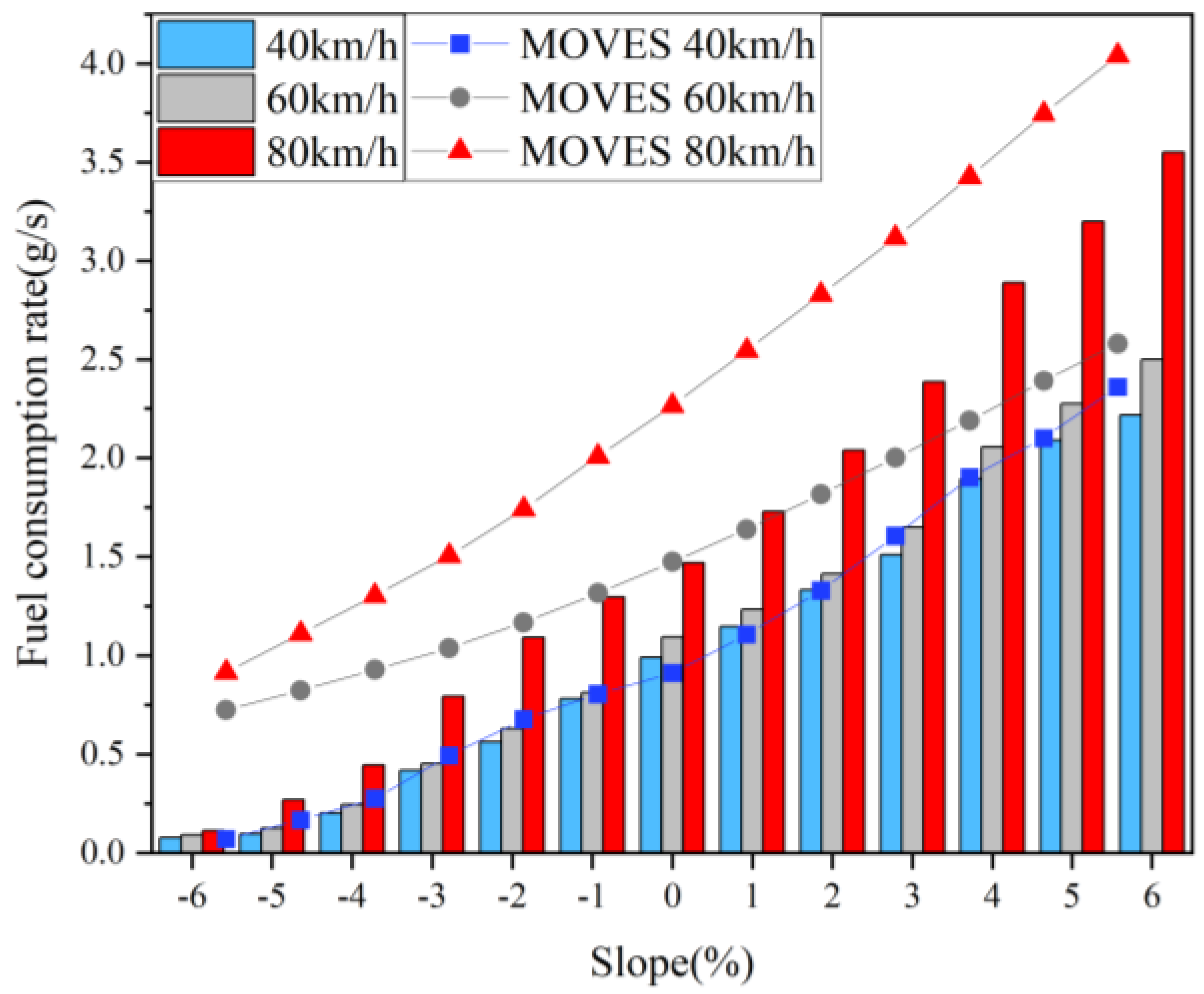
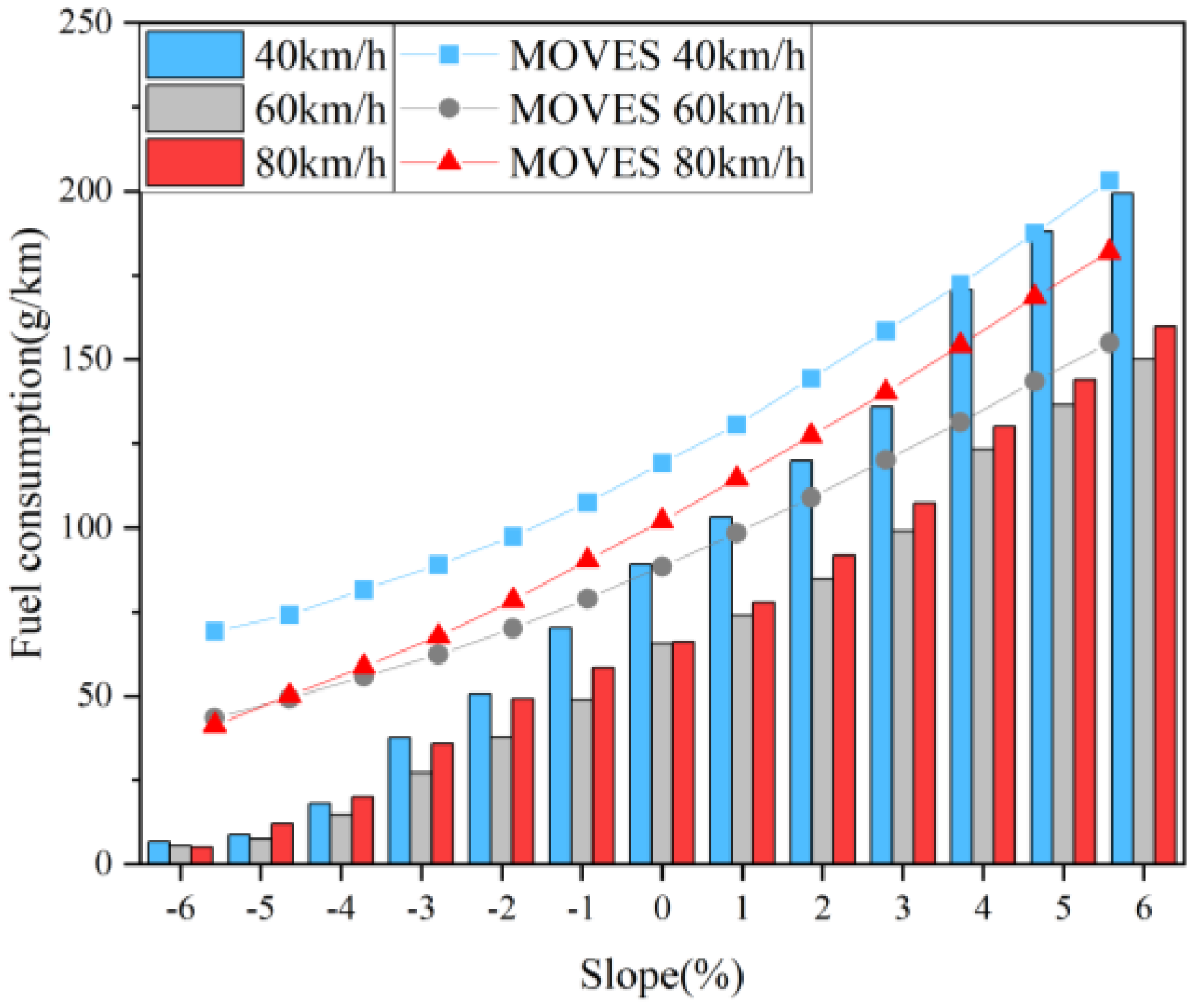
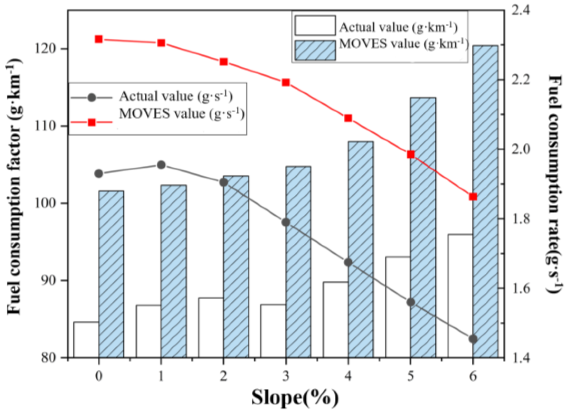
4.1. The Influence of Slope on Fuel Consumption Rate and Fuel Consumption Factor

Figure 7 shows the impact of the road gradient on the fuel consumption rate, with the experimental data aligning with the trends observed in the MOVES simulation results. Overall, as the gradient increases, the fuel consumption rate gradually rises. At the same gradient, higher vehicle speeds result in higher fuel consumption rates. Between −2% and +6%, the fuel consumption rate at 80 km/h is significantly higher than that at 60 km/h and 40 km/h. From +2% to +6%, the fuel consumption rates at 60 km/h and 40 km/h are relatively close, and they become closer as the gradient increases, suggesting that during low-to-medium speed climbing, the transmission gear is consistent, and both low and medium speeds fall within a more economical range, resulting in insignificant changes in fuel consumption. Between −6% and −2%, the fuel consumption rates at 80 km/h and 60 km/h are relatively close, while the fuel consumption rate at 40 km/h approaches zero. During downhill driving, the gradient resistance becomes a driving force. At low speeds, the gradient force can overcome road resistance; however, at medium-to-high speeds, the gradient force is insufficient to fully provide power, requiring additional power from the engine.

From a gradient of +3% to +4%, the fuel consumption rate increases the most, with increases of 25.1%, 24.5%, and 21.1% at speeds of 40 km/h, 60 km/h, and 80 km/h, respectively; the MOVES simulation data show increases of 18.7%, 10.1%, and 10%, respectively. At a gradient of +4%, the fuel consumption rate at 80 km/h is 1.40 times and 1.52 times that of 60 km/h and 40 km/h, respectively. When climbing uphill, at a speed of 60 km/h, a gradient of +4% results in a fuel consumption that is 1.87 times that on flat roads; at a speed of 80 km/h, a gradient of +4% results in a fuel consumption that is 1.96 times that on flat roads, with both MOVES simulation values being around 51%. These findings align with the conclusion drawn by Boriboonsomsin [8], who reported that an average gradient of +4% can reduce the fuel economy by a factor of 1.5 to 2 times. Boriboonsomsin’s study provides empirical support for our observations, reinforcing the significant impact that uphill gradients have on fuel consumption rates, particularly at steeper inclines.

Under the same gradient and slope length, higher vehicle speeds lead to higher fuel consumption but shorter traversal times through the slope; thus, it is necessary to consider the fuel consumption factor under constant speed conditions. Figure 8 shows the impact of gradient on the fuel consumption factor, with the highest factor at a speed of 40 km/h and the lowest at 60 km/h. It is not the case that the lowest speed results in the smallest emission factor when climbing hills; instead, the lowest fuel consumption factor occurs at medium-to-low speeds. At gradients of −6% and −5%, the fuel consumption factor at 80 km/h is less than that at 60 km/h; starting from −4%, the fuel consumption factor at 80 km/h is greater than that at 60 km/h, with the difference increasing as the gradient steepens. At speeds of 40 km/h, 60 km/h, and 80 km/h, the fuel consumption factors at a gradient of +6% are 2.23, 2.28, and 2.41 times those at 0%, respectively. At gradients of +6%, while the fuel consumption factor increases with speed compared to 0% gradient, the increase is less pronounced at medium-to-high speeds compared to the lowest speed of 40 km/h. Therefore, at this particular gradient, the fuel consumption factor at 60 km/h and 80 km/h is lower than at 40 km/h, although it is still higher than at a 0% gradient.

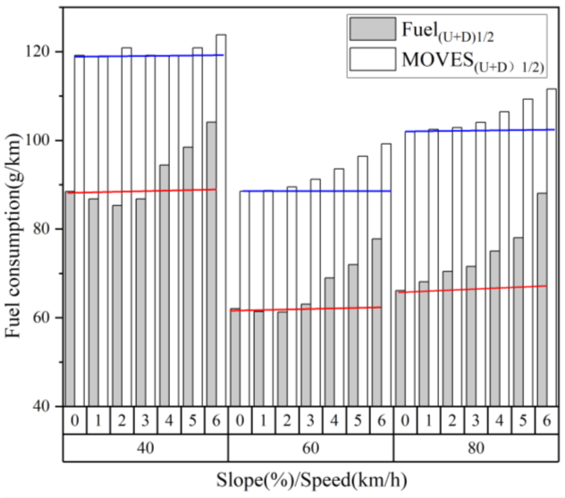
4.2. Differences in Average Fuel Consumption Factor Between Uphill/Downhill and Flat Roads

For roads, uphill and downhill are relative terms. As shown in Figure 7, uphill travel consumes more fuel than flat roads, while downhill travel saves fuel. To analyze whether the fuel saved during downhill driving can offset the additional fuel consumed during uphill driving, we compared the average fuel consumption factor for uphill and downhill driving with the same absolute gradient to the fuel consumption factor for flat roads (abbreviated as fuel0). In this paper, gradients without positive or negative signs refer to their absolute values.

Figure 9 shows the impact of different gradients on the combined fuel consumption factor for uphill and downhill driving. At gradients of 1% to 3%, fuel (U + D) 1/2 is not significantly different from fuel0, and MOVES (U + D) 1/2 is even closer to fuel0, suggesting that the fuel consumption factor saved during downhill driving can offset the additional fuel consumption factor during uphill driving. However, at gradients of 4% to 6%, both fuel (U + D) 1/2 and MOVES (U + D) 1/2 are significantly higher than fuel0. At a gradient of 6% and a speed of 80 km/h, fuel (U + D) 1/2 and MOVES (U + D) 1/2 are 1.33 and 1.1 times fuel0, respectively, indicating that the fuel consumption factor saved during downhill driving cannot offset the additional fuel consumption factor during uphill driving.

Based on the observations from Figure 8, we have found that the fuel consumption factor increases significantly with changes in the road gradient. Specifically, at a speed of 60 km/h, the fuel consumption factor for uphill gradients of +6% and downhill gradients of −6% is 2.28 times and 0.08 times, respectively, that of a 0% gradient. Within the range of +4% to +6% gradients, the fuel consumption factor doubles, whereas between −6% and −4% gradients, the change in the fuel consumption factor is insignificant. Furthermore, the rate of increase in the fuel consumption factor on uphill slopes is notably faster than the rate of savings on downhill slopes.

Theoretically, the increase and decrease in fuel consumption should be roughly balanced. However, during uphill driving, shifting gears or even reducing speed is necessary, which often means that the increase in fuel consumption surpasses the savings on downhill slopes, leading to an overall higher fuel consumption along the route. On gentle slopes, the fuel consumption savings on downhill slopes roughly balance out the increase on uphill slopes. On steep slopes, it can be considered that the increase in fuel consumption on uphill slopes surpasses the savings on downhill slopes. This is because maintaining the current speed while climbing steep slopes requires greater acceleration, resulting in a significant increase in fuel consumption on uphill slopes.

5. The Impact of Slope on Fuel Consumption in Real-World Scenarios

Analysis of Fuel Consumption Under Actual Vehicle Speed Conditions

In practical situations, different gradients have varying effects on the motion state of vehicles. The median vehicle speeds under different gradient conditions, along with the corresponding Vehicle Specific Power (VSP) and fuel consumption rates, are analyzed. The median vehicle speeds (hereinafter referred to as actual speeds) under different gradients from the experiments are used as inputs for the MOVES model to simulate and obtain simulated fuel consumption values.

The median vehicle speeds at different gradients exclude extreme driving conditions and better represent the operating speeds on those gradients. Figure 10 illustrates the impact of different gradients on the combined fuel consumption factor for uphill and downhill driving. Figure 10A shows that under downhill conditions, the greater the gradient, the slower the vehicle speed. On flat roads, the vehicle speed reaches its maximum. On uphill roads, the vehicle speed gradually decreases as the gradient increases. The smaller the absolute value of the gradient, the higher the vehicle speed, and conversely, the larger the absolute value of the gradient, the lower the speed, overall presenting a positive parabolic shape. Between −6% and −1%, an increase in the gradient by 1% results in an increase in the vehicle speed by 3.66 km/h; between −3% and 0%, the increase in speed is not significant. Between 1% and 6%, an increase in the gradient by 1% results in a decrease in the vehicle speed by 5.42 km/h. When the absolute values of the gradients are equal, the vehicle speeds on downhill slopes are higher than those on uphill slopes. Analyzing the impact of gradients on the fuel consumption at a constant speed for the same gradient reveals significant differences.

Analyzing the impact of different gradients on the VSP and fuel consumption in Figure 10B, the overall trend of the actual fuel consumption distribution aligns with that of the MOVES model. From −6% to +3%, the VSP value increases as the gradient increases. When the gradient reaches +3%, further increases in the gradient do not significantly alter the VSP value. At a gradient of −3%, the VSP value transitions from negative to positive. Compared to flat roads, gradients of +2% result in a 42% increase in the VSP and a 41% increase in the fuel consumption rate, while gradients of +4% lead to a 49% increase in the VSP and a 51% increase in the fuel consumption rate.

Between gradients of −4% and +4%, each 1% increase in the gradient results in a 0.32 g/s increase in the fuel consumption. The highest fuel consumption occurs at a gradient of +4%. As the gradient further increases, the VSP value remains unchanged, while the actual fuel consumption begins to decline. This is attributed to the engine power approaching its maximum at medium-to-high gradients, leading to a reduction in the gear and vehicle speed, and an increase in the torque. Combined with the engine’s universal characteristic curve, the load rate increases further, improving the fuel economy.

Figure 11 presents the combined fuel consumption factor and fuel consumption rate for uphill and downhill driving at different gradients. By averaging the actual fuel consumption for uphill and downhill driving at various speeds, the impact of gradients on the fuel consumption is analyzed based on both the fuel consumption rate and fuel consumption factor, with MOVES model data used for validation. The trend in the MOVES simulation results is consistent with that under actual conditions. It is found that, in practical situations, there is little difference in the fuel consumption rate between gradients of 0% and 1%. The average fuel consumption rate for uphill and downhill driving decreases as the gradient increases, while the average fuel consumption for both increases with increasing gradient. Analyzing the average fuel consumption factor for uphill and downhill driving, changes are not significant between gradients of 0% and 3%, suggesting that the fuel savings on downhill slopes can offset the additional fuel consumption on uphill slopes. At gradients of 4% to 6%, the increase in the fuel consumption factor on uphill slopes surpasses the savings on downhill slopes, resulting in an overall increase in the fuel consumption factor with increasing gradient.

Starting from a gradient of 1%, with each subsequent 1% increase in gradient, the average fuel consumption factor for uphill and downhill driving decreases by approximately 7%. The growth of the fuel consumption factor is relatively slow at gradients of 0% to 3%, but it begins to increase significantly when the gradient exceeds 3%. At a gradient of 6%, the actual fuel consumption factor is 13.4% higher than that on flat roads, while the MOVES-simulated fuel consumption factor is 18.5% higher. When the gradient is between 4% and 5%, both the actual data and MOVES-simulated data show an intersection in trends for the fuel consumption rate and fuel consumption factor, indicating that, as the vehicle speed decreases, the fuel consumption rate also decreases, but the overall fuel consumption increases due to a longer climbing time.

An increase in the gradient leads to a significant reduction in the vehicle speed, and lower speeds are prone to causing congestion on slopes. Considering both the vehicle speed and energy consumption, at gradients of 3% and 4%, the actual fuel consumption factors and MOVES-simulated fuel consumption factors are 2.7% and 6.1%, and 3.1% and 6.2% higher than those on corresponding flat roads, respectively. At gradients of 3% and 4%, the median vehicle speeds for uphill and downhill driving reach 73 km/h and 65 km/h, respectively. A gradient of 3% represents the optimal balance between the overall fuel consumption and vehicle speed. Beyond 3%, the overall fuel consumption increases significantly, and the vehicle speed decreases drastically.

6. Conclusions

Through actual road experiments conducted in plateau and mountainous areas, 66,000 pieces of data were collected. The impact of the road gradient on the fuel consumption was analyzed, and the actual VSP distribution obtained from the experiments was used as an input for the MOVES model. Finally, the simulation results were validated against the experimental results.

• Extreme acceleration and deceleration primarily occur on sections with gentle gradients. As the absolute value of the gradient increases, both the vehicle speed and acceleration/deceleration become smoother. High fuel consumption rates are concentrated mainly around gradients of 4%.
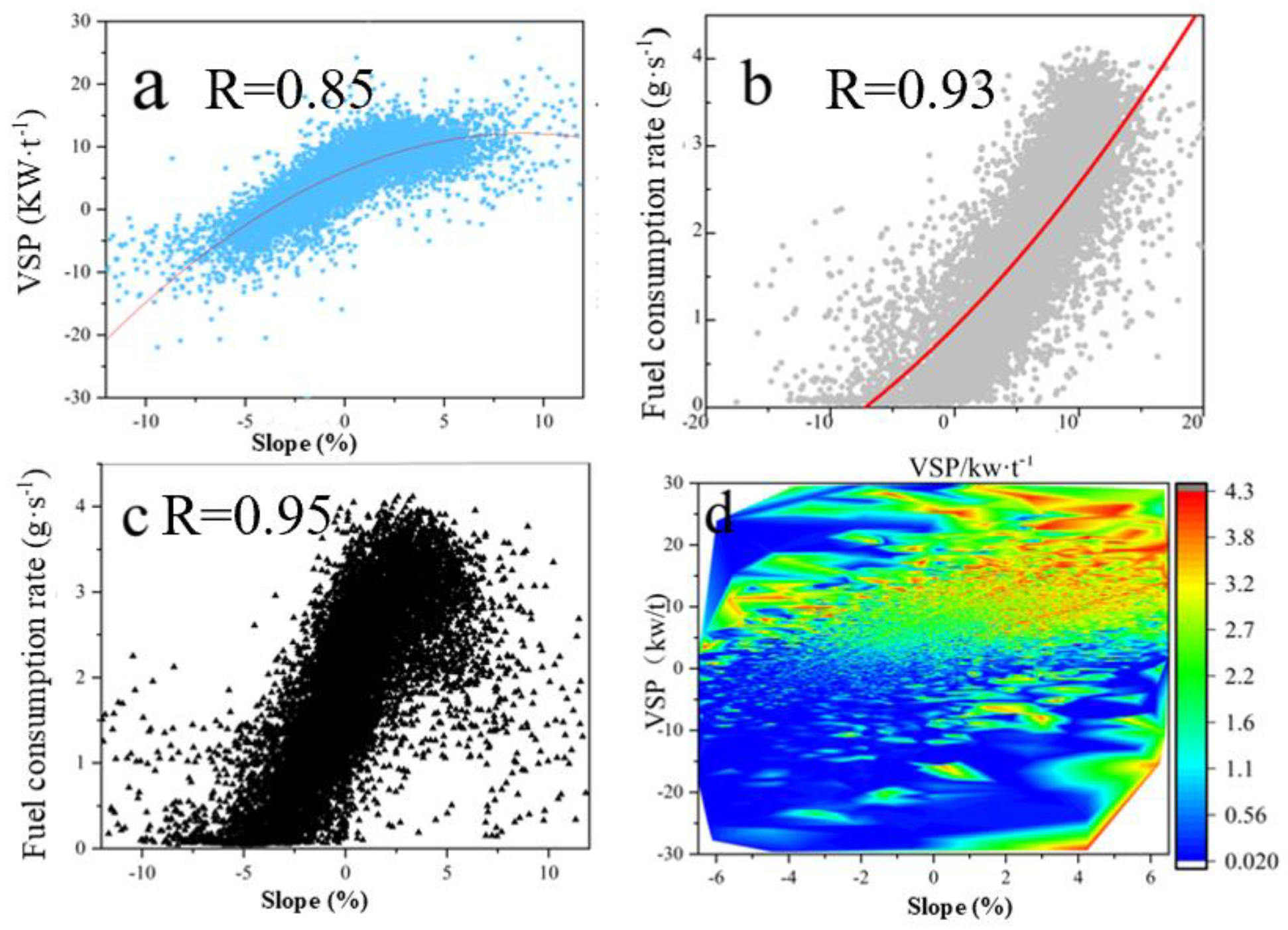
• The road gradient has a significant impact on the VSP and fuel consumption of light-duty diesel vehicles. When the gradient ranges from −5% to +5%, there is a good parabolic relationship between the gradient and VSP, a linear relationship between the gradient and fuel consumption, and an inverse parabolic relationship between the VSP and fuel consumption. These three factors exhibit a good positive correlation. Models based on the VSP have good adaptability in plateau and mountainous areas.
• During uphill driving, the fuel consumption factor is lowest at a speed of 60 km/h and highest at 40 km/h. It is noteworthy that, contrary to intuition, adopting medium-to-high speeds (such as 80 km/h) when climbing hills can result in a lower fuel consumption factor compared to that at lower speeds (like 40 km/h). This is because, at certain gradients and under specific conditions, higher speeds may optimize engine efficiency and reduce the overall fuel consumption, despite the increased workload. Therefore, the recommendation should be adjusted to suggest adopting speeds within the medium-to-high range when climbing hills, particularly where conditions favor such an approach.
• Between gradients of 1% to 3%, the fuel consumption factor saved during downhill driving is considered to offset the additional fuel consumption factor on uphill stretches. However, between gradients of 4% and 6%, the increase in the fuel consumption factor on uphill stretches is considered to surpass the savings in fuel consumption during downhill driving. This paper provides a reference for road gradient design from an energy perspective, with the optimal gradient for the vehicle speed and energy consumption being 3%.

7. Limitations

The application of the MOVES model in the special environment of plateau and mountainous regions indeed presents some limitations. Firstly, the high altitude significantly affects the engine performance, such as causing power reduction and changes in the fuel consumption rate due to thinner air, which may not be fully considered in the default settings of the MOVES model. Secondly, the interference of complex terrain on vehicle driving conditions, such as frequent uphill and downhill driving and sharp turns, also affects the vehicle fuel consumption and emission characteristics, and the MOVES model may have certain limitations in simulating these complex conditions.

Furthermore, the MOVES model faces challenges when simulating the vehicle performance under extreme weather conditions (such as low oxygen, low temperature, and strong winds). For example, a low-oxygen environment affects engine combustion efficiency, while low temperatures may lead to poor fuel atomization and increased emissions, which may not be accurately reflected in the simulations of the MOVES model.

In terms of potential sources of error, the uncertainty of the input data for the MOVES model is an important factor. For instance, the accuracy and completeness of parameters such as the road gradient, vehicle load, and driver behavior have a significant impact on the model results. If these data are inaccurate or incomplete, the simulation results of the model will also be affected. Additionally, the sensitivity of model parameter settings is another potential source of error. For example, the value ranges of key parameters such as emission factors and fuel consumption rates have a direct impact on the simulation results, and there may be some uncertainty in the values of these parameters. In future research, we will continue to explore ways to improve the MOVES model to enhance its accuracy and reliability in predicting fuel consumption for light-duty diesel vehicles in plateau and mountainous regions.

References

1. Liu, J.; Ge, Y.; Wang, X.; Hao, L.; Tan, J.; Peng, Z.; Zhang, C.; Gong, H.; Huang, Y. On-board measurement of particle numbers and their size distribution from a light-duty diesel vehicle: Influences of VSP and altitude. J. Environ. Sci. 2017, 57, 238–248. [Google Scholar] [CrossRef] [PubMed]
2. Peng, F.; Song, G.H.; Ying, H.; Yu, L. Energy consumption and CO2 emission model for hybrid electric vehicles based on actual traffic conditions. Transp. Syst. Eng. Inf. 2022, 22, 316–326. [Google Scholar]
3. Luján, J.M.; Bermúdez, V.; Dolz, V.; Monsalve-Serrano, J. An assessment of the real-world driving gaseous emissions from a Euro 6 light-duty diesel vehicle using a portable emissions measurement system (PEMS). Atmos. Environ. 2018, 174, 112–121. [Google Scholar] [CrossRef]
4. Kwon, S.; Park, Y.; Park, J.; Kim, J.; Choi, K.H.; Cha, J.S. Characteristics of on-road NOx emissions from Euro 6 light-duty diesel vehicles using a portable emissions measurement system. Sci. Total Environ. 2017, 576, 70–77. [Google Scholar] [CrossRef] [PubMed]
5. Tang, R.X. Research on Traffic Safety Prediction for Mountainous Expressway Based on Traffic Accident Analysis. Master’s Thesis, Chongqing Jiaotong University, Chongqing, China, 2019. [Google Scholar]
6. Faria, M.V.; Duarte, G.O.; Varella, R.A.; Farias, T.L.; Baptista, P.C. How do road grade, road type and driving aggressiveness impact vehicle fuel consumption? Assessing potential fuel savings in Lisbon, Portugal. Transp. Res. Part D Transp. Environ. 2019, 72, 148–161. [Google Scholar] [CrossRef]
7. Wu, T.; Han, X.; Zheng, M.M.; Ou, X.; Sun, H.; Zhang, X. Impact factors of the real-world fuel consumption rate of light duty vehicles in China. Energy 2019, 190, 116388. [Google Scholar] [CrossRef]
8. Boriboonsomsin, K.; Barth, M. Impacts of Road Grade on Fuel Consumption and Carbon Dioxide Emissions Evidenced by Use of Advanced Navigation Systems. Transp. Res. Rec. J. Transp. Res. Board 2009, 2139, 21–30. [Google Scholar] [CrossRef]
9. Frey, H.C.; Zhang, K.; Rouphail, N.M. Fuel Use and Emissions Comparisons for Alternative Routes, Time of Day, Road Grade, and Vehicles Based on In-Use Measurements. Environ. Sci. Technol. 2008, 42, 2483–2489. [Google Scholar] [CrossRef] [PubMed]
10. Loulizi, A.; Rakha, H.; Bichiou, Y. Quantifying grade effects on vehicle fuel consumption for use in sustainable highway design. Int. J. Sustain. Transp. 2017, 12, 441–451. [Google Scholar] [CrossRef]
11. Kanarachos, S.; Mathew, J.; Fitzpatrick, M.E. Instantaneous vehicle fuel consumption estimation using smartphones and recurrent neural networks. Expert Syst. Appl. 2019, 120, 436–447. [Google Scholar] [CrossRef]
12. Zhang, J.H.; Li, K.Q.; Xu, B.; Li, H. Estimation of Vehicle Transient Fuel Consumption Based on Least Squares Method. Automot. Eng. 2018, 40, 1151–1157. [Google Scholar]
13. U.S. Environment Protection Agency. MOVES 2014a User Guide; Assessment and Standards Division Office of Transportation and Air Quality: Washington, DC, USA, 2015. [Google Scholar]
14. Liu, H.; Li, H.; Rodgers, M.O.; Guensler, R. Development of road grade data using the United States geological survey digital elevation model. Transp. Res. 2018, 92, 243–257. [Google Scholar] [CrossRef]
15. Wang, X.M. Experimental Research on Road Gradient Measurement Methods. Agric. Equip. Veh. Eng. 2015, 53, 6–11. [Google Scholar]
16. Liu, H.; Rodgers, M.O.; Guensler, R. Impact of road grade on vehicle speed-acceleration distribution, emissions and dispersion modeling on freeways. Transp. Res. Part D Transp. Environ. 2019, 69, 107–122. [Google Scholar] [CrossRef]
17. Jiménez-Palacios, J.L. Understanding and quantifying motor vehicle emissions with vehicle specific power and TILDAS remote sensing. Mass. Inst. Technol. 1999, 1–360. Available online: https://dspace.mit.edu/handle/1721.1/44505 (accessed on 12 January 2025).
18. Pang, R.; Jian, X.C.; Meng, X.; Jin, D. Comprehensive Fuel Consumption Model for Light-duty Vehicles Based on Specific Power in Typical Mountainous Cities. Sci. Technol. Eng. 2018, 18, 6. [Google Scholar]
Figure 1. Test route. (The red lines represent the route, with the altitude decreasing from the start point to the end point).
Atmosphere 16 00143 g001
Figure 2. Flowchart for extracting slope information.
Atmosphere 16 00143 g002
Figure 3. The influence of slope on the vehicle’s motion state.
Atmosphere 16 00143 g003
Figure 4. Distribution diagram of VSP (a) and fuel consumption (b) under different vehicle speeds and accelerations.
Atmosphere 16 00143 g004
Figure 5. Relationship diagram of slope, VSP, and fuel consumption. (a) (VSP &Slope); (b) (Fuel consumption & VSP); (c) (Slope & Fuel consumption); (d) (Slope & VSP).
Atmosphere 16 00143 g005
Figure 6. Differences between uphill/downhill roads and flat roads.
Atmosphere 16 00143 g006
Figure 7. The influence of slope on fuel consumption rate.
Atmosphere 16 00143 g007
Figure 8. The influence of slope on fuel consumption factor.
Atmosphere 16 00143 g008
Figure 9. Impact of different slopes on the comprehensive fuel consumption factor for uphill and downhill travel (The red lines represent the horizontal levels of Fuel(U+D)1/2, while the blue lines represent the horizontal levels of MOVES(U+D)1/2).
Atmosphere 16 00143 g009
Figure 10. Impact of different slopes on the composite fuel consumption factor for ascending and descending roads (The blue triangles represent the corresponding speed values at different gradients).
Atmosphere 16 00143 g010
Figure 11. Comprehensive fuel consumption factor and fuel consumption rate for uphill and downhill travel at different slopes.
Atmosphere 16 00143 g011