A Time-Dependent Intrinsic Correlation Analysis to Identify Teleconnection Between Climatic Oscillations and Extreme Climatic Indices Across the Southern Indian Peninsula

Abstract

Large-scale climatic oscillations (COs) modulate extreme climate events (ECEs) globally and can trigger the Indian summer monsoons and associated ECEs. In this study, we introduced a Time-dependent Intrinsic Correlation (TDIC) analysis to quantify teleconnections between five major COs—the El Niño–Southern Oscillation (ENSO), Atlantic Multidecadal Oscillation (AMO), Indian Ocean Dipole (IOD), North Atlantic Oscillation (NAO), and Pacific Decadal Oscillation (PDO)—and multiple extreme climate indices (ECIs) over the southern Indian Peninsula. Complete ensemble empirical mode decomposition with adaptive noise (CEEMDAN) was employed to decompose COs and ECIs into intrinsic mode functions across varying timescales, enabling a dynamic TDIC assessment. The results revealed statistically significant correlations between COs and ECIs, with the strongest influences in low-frequency modes (>10 years). Distinct COs predominantly modulate specific ECIs (e.g., ENSO with monsoon rainfall extremes; AMO and PDO with temperature extremes). These findings advance the understanding of Indian climate system dynamics and support the development of improved ECE forecasting models.

1. Introduction

Global temperatures are projected to rise by 2.8 °C by the end of this century, with profound impacts on atmospheric water content, arctic warming, snowmelt water, and the frequency and intensity of extreme climate events [1,2,3]. Climate indices distill complex atmospheric data—past, present, and projected—into concise metrics that facilitate the communication of specific circulation patterns and their societal and environmental impacts. These indices are designed to provide objective, unbiased assessments of the observed and anticipated climate variability and change [4,5]. The Expert Team on Climate Change Detection and Indices (ETCCDI), established under the World Meteorological Organization (WMO), developed a widely adopted set of 27 core climate indices that provide a rigorous, quantitative representation of moderate climate extremes. These indices are typically expressed as annual time series, with each value reflecting the frequency, intensity, or duration of threshold-based or percentile-defined events within a given year. Over the past two decades, numerous studies have systematically analyzed trends, abrupt change points, and persistence in these ETCCDI across global and regional scales, enabling the robust detection and attribution of climate variability and change [6,7,8,9,10,11,12].

In the Indian context, numerous studies have investigated climate extremes and variability, yielding diverse conclusions shaped by differences in datasets, spatial domains, and analytical methods [11]. Large-scale climatic oscillations (COs), such as the El Niño–Southern Oscillation (ENSO), Atlantic Multidecadal Oscillation (AMO), Indian Ocean Dipole (IOD), North Atlantic Oscillation (NAO), and Pacific Decadal Oscillation (PDO), exert well-documented influences on global and regional climate variability, particularly modulating the Indian summer monsoon and associated rainfall patterns [13,14,15]. Earlier investigations of hydroclimatic teleconnections relied on stationary statistical measures like Pearson correlations and mutual information to quantify relationships between COs and hydro-meteorological variables [15,16]. However, a comprehensive understanding of these interactions requires a multiscale analysis to disentangle scale-specific influences and non-stationary dynamics [14].

The traditional power spectral analysis or cross-spectral analysis was found to be useful for capturing the dominant frequency of natural processes. To simultaneously handle the resolution in the both time and frequency domain, recent studies have suggested the wavelet transform method [17,18]. The discrete wavelet transform, its continuous variant, and wavelet coherence were reported to be powerful in analyzing the teleconnection between hydrologic and climatic variables [19,20,21,22,23]. Apart from difficulties in the selection of appropriate wavelet functions, fixing the optimal number of scales is also found to be challenging in the use of wavelets [24]. Even though Morlet is identified as an approved choice, as the mother wavelet in the continuous wavelet variants, it is unable to distinctly separate the process scales, which is often disadvantageous in capturing the scale-specific information, which is more appealing for extending the traditional teleconnection studies to predictions. In this context, decomposition methods like Empirical Mode Decomposition (EMD), which can separate a series to a distinct optimal number of process scales, are recommended. Many research projects have presented a systematic comparison of the traditional spectral analysis method to Hilbert Huang Transform (HHT), involving EMD as the prime step, stating their limitations and strengths in handling nonlinear and non-stationary series [25]. Time-dependent running (dynamic) correlations between the corresponding modes from two candidate series can be performed, which again offer the advantage of accounting for the non-stationarity aspect effectively with a piece-wise running window approach.

The HHT is a two-phase time frequency transformation method, introduced by Huang et al. Its first part is EMD, which is a fully data-adaptive technique that decomposes non-stationary and nonlinear time series into intrinsic mode functions (IMFs) and a residual trend, each characterized by distinct oscillatory timescales [25]. To address EMD’s limitations—particularly mode mixing, where disparate frequencies contaminate individual IMFs—noise-assisted variants have been developed, including the Ensemble EMD (EEMD), complete ensemble EMD with adaptive noise (CEEMDAN), and Improved CEEMDAN (I-CEEMDAN) [26,27,28,29,30]. In the second phase, the IMFs are subjected to a Hilbert spectral analysis, which deduces the time–frequency–amplitude spectrum and marginal spectrum. The instantaneous amplitude and frequency derived are used for a dynamic correlation procedure, namely the Time-Dependent Intrinsic Correlation (TDIC), for teleconnection studies.

A seminal advancement came from Chen et al. [31], who extended the EMD to a time–frequency correlation analysis, introducing a TDIC framework that quantifies scale-specific, time-localized relationships between paired geophysical signals. Since its inception, the TDIC has been widely adopted across disciplines to explore multiscale interactions in climate, hydrology, and environmental systems [32,33,34,35,36]. By revealing how climatic oscillations modulate extreme climate indices (ECIs) at specific frequencies and evolutionary phases, the TDIC enables the robust detection of teleconnection mechanisms. Such insights enhance the predictability of temperature extremes, precipitation anomalies, and high-impact weather events, supporting proactive adaptation and risk mitigation strategies in a warming climate.

South Peninsular India (SPI) exhibits diverse climatic regimes driven by its complex topography and proximity to the Indian Ocean. The region is broadly characterized by warm, humid conditions, with coastal areas experiencing a tropical maritime climate marked by high humidity and heavy rainfall during the southwest monsoon (June–September). The Western Ghats, a prominent orographic barrier, significantly modulate monsoon dynamics, inducing sharp rainfall gradients: windward slopes in Kerala, Karnataka, and Goa receive orographic precipitation exceeding 3000 mm annually, while leeward interiors of the Deccan Plateau remain relatively arid [37]. This interplay renders SPI highly vulnerable to extreme climate events, including heatwaves, intense rainfall, droughts, and floods [23]. The Indian summer monsoon is strongly modulated by large-scale COs, including the ENSO, IOD, AMO, PDO, and NAO [13,19]. However, studies explicitly linking COs to ECIs over SPI remain scarce. To the authors’ knowledge, no prior investigation has applied the TDIC within a CEEMDAN framework to characterize scale-specific, time-localized teleconnections between COs and ECIs across the Indian Peninsula. This gap underscores the novelty of the present study in advancing the hydroclimatological understanding of monsoon-driven extremes. Accordingly, the specific objectives of this work are as follows:

(i)

To compute a suite of ETCCDI-based ECIs for SPI’s homogeneous monsoon region.

(ii)

To resolve the dominant periodicities of ECIs and COs using CEEMDAN.

(iii)

To quantify dynamic, scale-resolved associations between ECIs and COs via the CEEMDAN-TDIC framework.

2. Materials and Methods

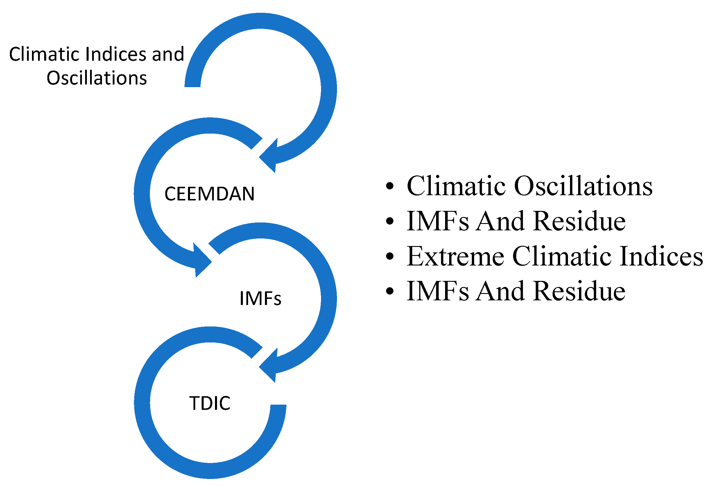
The methodological workflow is illustrated in Figure 1. Daily gridded datasets of precipitation (PRCP), maximum temperature (TX), and minimum temperature (TN) were obtained from the India Meteorological Department (IMD) for all grid points (0.25° × 0.25° resolution) spanning India. These data were stratified according to the five homogeneous monsoon regions delineated by the IMD. For each region, grid points were selected, and areal averages were computed to yield region-specific time series. Subsequently, the 27 core ETCCDI indices were calculated for SPI’s homogeneous region using the RClimDex (version 1).

RClimDex is a library in R developed and maintained by ETCCDI under the WMO. It is one of the most widely used tools worldwide for calculating the 27 core ETCCDI climate extremes indices (plus a few additional ones) from daily precipitation, maximum temperature, and minimum temperature data. The package performs basic quality control on daily data (outliers, unreasonable values, duplicates, etc.) and handles missing values according to ETCCDI standards. The package can be installed from the official ETCCDI website or GitHub mirrors (https://github.com/ECCC-CDAS/RClimDex) (accessed on 12 January 2023).

2.1. CEEMDAN

In the complete EEMD with adaptive noise, an addition of noise series is made at every step of the decomposition.

• Employ EMD for M resamples $X_m\left(t\right)=X\left(t\right)+{\epsilon }_0{w}_m\left(t\right)$ and extract the 1st component

  $$\overline{IM{F}_1\left(t\right)}={\displaystyle \frac{1}{M}}{\sum }_{m=1}^{M}IM{F}_m\left(t\right)$$

  (1)

  where m = 1, 2, …, M is the noise measure for this initial stage.
  This step demonstrates that the first mode derived from CEEMDAN is identical to that obtained from EEMD.
• Find the initial residual as $R_1\left(t\right)=X\left(t\right)-\overline{\overline{IM{F}_1\left(t\right)}}$.
• Decompose the resamples, ${R_1}_m\left(t\right)=R_1\left(t\right)+{\epsilon }_1{E}_1\left(w_m\right(t\left)\right)$, until their first EMD component evolves. Subsequently, find

  $$\overline{\overline{IM{F}_2\left(t\right)}}={\displaystyle \frac{1}{M}}\sum _{m=1}^M{E}_1\left[R_1\right(t)+{\epsilon }_1{E}_1(w_m\left(t\right)]$$

  (2)

  where Ek(·) is the operation of kth component by EMD; ${\epsilon }_1$ is the noise measure for k = 1.
• Find the kth residue as

  $$R_k\left(t\right)=R_{k-1}\left(t\right)-\overline{\overline{IM{F}_k\left(t\right)}}$$

  (3)

  for k = 2, 3, …, K, where the IMFs are obtained by CEEMDAN.
• Estimate $R_k\left(t\right)+{\epsilon }_k{E}_k\left(w_m\right(t\left)\right)$ and

  $$\overline{\overline{IM{F}_{k+1}\left(t\right)}}={\displaystyle \frac{1}{M}}\sum _{m=1}^M{E}_1\left[R_k\right(t)+{\epsilon }_k{E}_k(w_m\left(t\right)]$$

  (4)

  $$R_K\left(t\right)=X\left(t\right)-\sum _{k=1}^K\overline{\overline{IM{F}_k\left(t\right)}}$$

  (5)
• Repeat from (4) for subsequent k-values until the residual is a monotonical trend or a single peak has evolved.
  The final residual becomes

  $$X(t)={\displaystyle \sum _{k=1}^K\left[\overline{\overline{IM{F}_k(t)}}\right]}+R_K(t)$$

  (6)

Geophysical processes are typically influenced by numerous potential causal variables, making it essential to examine the relationships between these processes and their corresponding input variables. Over the years, researchers have developed various extensions of Empirical Mode Decomposition (EMD), including noise-assisted versions, capable of simultaneously analyzing multiple time series data points. For instance, Rilling et al. [38] introduced bi-dimensional EMD, while Rehman and Mandic [39] proposed tri-dimensional EMD. Among these advancements, the Multivariate Empirical Mode Decomposition (MEMD) introduced by Rehman and Mandic [40] represents the most generalized framework, enabling the simultaneous decomposition of multiple signals with enhanced efficiency and accuracy.

2.2. TDIC Method

This multiscale correlation procedure uses EMD or its improvisations to decompose the time series of concern to different scales. The correlation estimates are produced by fixing the window length adaptively, ensuring the stationary feature of the time series within it based on the instantaneous period (IP). As illustrated in Figure 2, the steps are as follows:

• Invoke CEEMDAN to decompose the pair of series to different modes.
• Select the IMF pairs with comparable periodicity.
• Determine the instantaneous frequencies (IFs) of IMF pairs using Hilbert spectral analysis and hence IPs.
• Compute the minimum moving window length (t_d) as the maximum of IPs at each instant t_k, i.e., $t_d={Max (T}_{1,i}\left(t_k\right),T_{2,i}\left(t_k\right))$ where $T_{1,i}$ and $T_{2,i}$ are IPs.
• Find the size of the moving window ${t_w}^n=\left[t_k-{\displaystyle \frac{n{t}_d}{2}}:t_k+{\displaystyle \frac{n{t}_d}{2}}\right]$ where n is chosen as unity.
• Assume IMF₁ and IMF₂ are two IMFs with comparable mean periods but belong to the different series in the pair. The TDIC measure can be estimated at any instant, ${{R_i(t}_w}^n)=Corr\left({{{IMF}_{1,i}(t}_w}^n),{{{IMF}_{2,i}(t}_w}^n)\right)$, where Corr is Pearson correlation.
• Use Student t-test to find statistical significance of correlations.
• Repeat steps 4 to 7 in an iterative manner until the window crosses the end points of the signal.

The TDIC matrix is visualized as a triangular plot, with the x-axis representing the midpoint of the sliding time window and the y-axis denoting window length (in years). The correlation at the triangle’s apex corresponds to the global (full-length) correlation when the window equals the entire time series duration [30]. The base of the triangle displays the IFs of the aligned IMFs, with a systematic upward shift observed for lower-frequency (longer-period) IMFs, reflecting their broader temporal support. This structure enables robust detection of scale-specific, time-localized correlations between paired variables across geophysical domains [31,35].

3. Study Area and Data

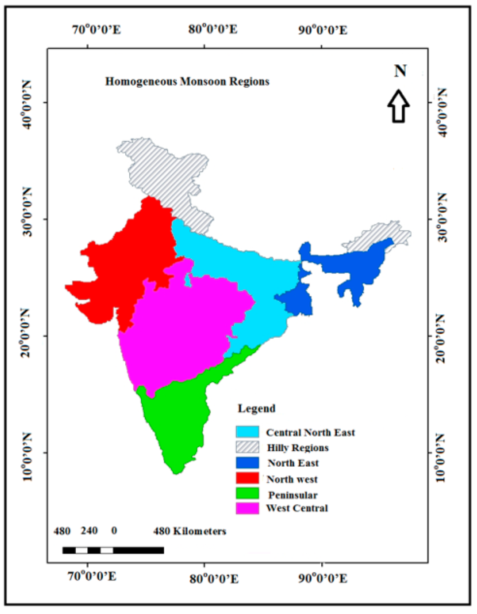
The Indian mainland is divided into five homogeneous rainfall regions based on the clustering of meteorological subdivisions defined by the Indian Institute of Tropical Meteorology (IITM), Pune. This study focuses on SPI—a climatically diverse zone bounded by the Arabian Sea to the west, the Indian Ocean to the south, and the Bay of Bengal to the east (Figure 3). This tri-coastal configuration enables a direct and rapid oceanic influence on the regional climate. SPI encompasses a spectrum of hydroclimatic regimes: Kerala, the “gateway of the Indian monsoon”, receives the earliest onset of southwest monsoon rains annually; Tamil Nadu and parts of Telangana experience relatively low rainfall; Vidarbha is drought-prone; and major urban centers like Chennai are vulnerable to extreme precipitation and flooding. The region has endured stark interannual contrasts, exemplified by severe drought in 2017 and catastrophic floods in 2018. Although SPI has a diverse climate shaped by its geography, consisting of coastal areas, mountains, and plains, there is a strong effect of the monsoon system on the climate of southern India that suggests a global teleconnection [41].

Daily gridded precipitation and temperature data (0.25° × 0.25° resolution) from the IMD for the period 1951–2015 were used to compute the 27 core GitHub indices for SPI’s homogeneous region using the RClimDex package. Quality control, outlier detection, and homogeneity checks were applied following ETCCDI protocols. We have considered 11 of the most relevant monthly scale indices (see

Table 1. List of monthly indices used in this study.

Index	Description
TX90p	Warm days
TN90p	Warm nights
TX10p	Cool days
TN10p	Cool night
TNn	Minimum of Tmin
TNx	Maximum of Tmin
TXn	Minimum of Tmax
TXx	Maximum of Tmax
DTR	Diurnal temperature range
Rx5 Day	Max 5-day precipitation
Rx1 Day	Max 1-day precipitation

) for our analysis, as it is already well proven that the teleconnections of the CO dataset manifest more at a monthly time scale [12,42].

All over the Indian subcontinent, 277 grid points (each associated with a given latitude and longitude) were found, where the data for both variables are accessible without any missing values. The 65 years of data on the selected climatic oscillations, namely the ENSO, AMO, IOD, NAO and PDO, were acquired from https://psl.noaa.gov/data/climateindices/list/ (accessed on 20 December 2022).

4. Results

As previously mentioned, first, the ECIs were computed, and then the ECI signals were decomposed into IMFs. Eventually, the correlations of the IMFs of ECIs with the IMFs of the climatic oscillations were obtained. The associated results for each step are presented in the following sections.

4.1. Extreme Climatic Indices

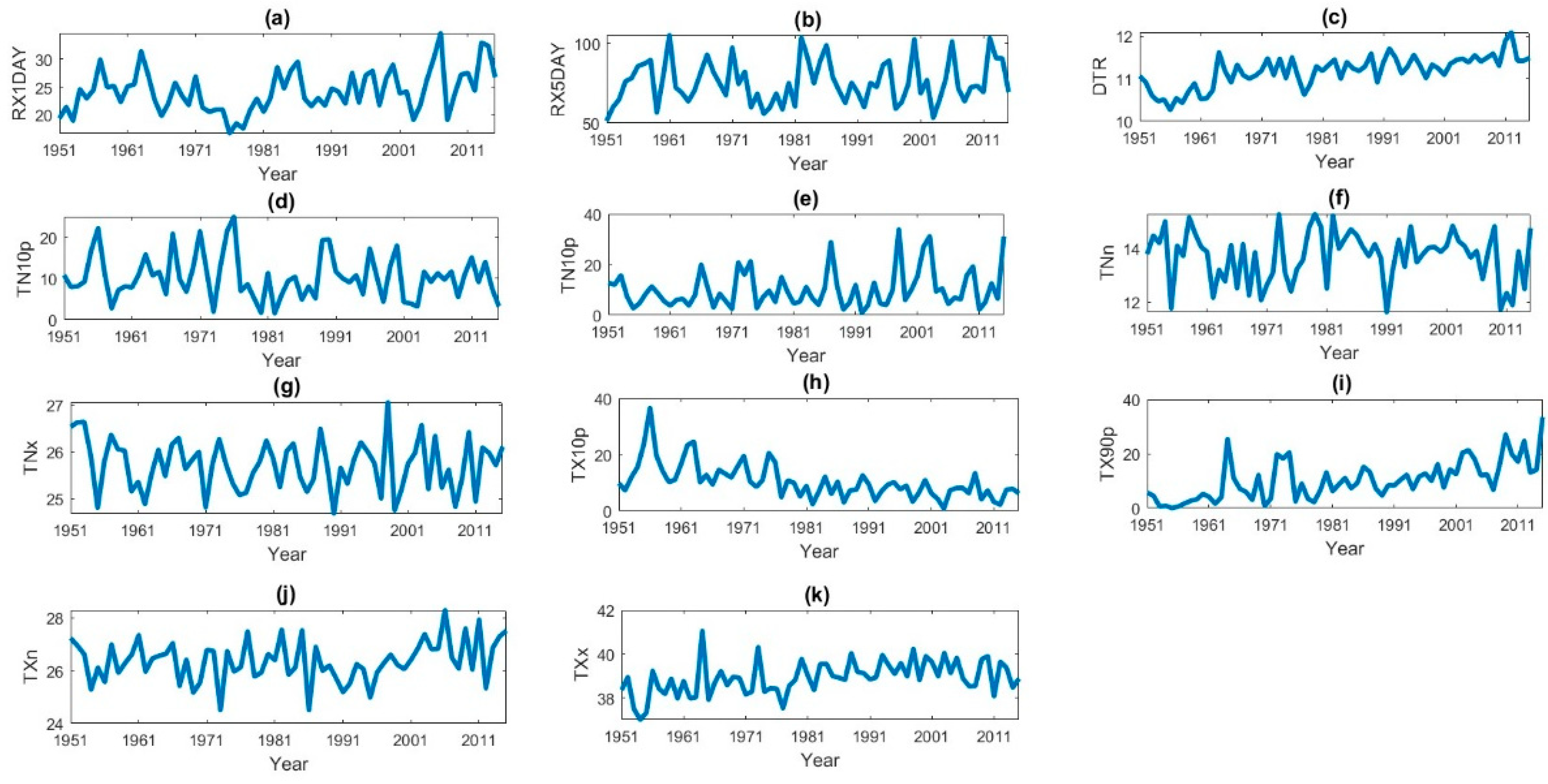
Among the 27 ETCCDI indices calculated from RClimDex, the monthly series of the TXx (max Tmax), TNx (max Tmin), TXn (min Tmax), TNn (min Tmin), TN10p (cool nights), TX10p (cool days), TN90p (warm nights), TX90p (warm days), DTR (diurnal temperature range), Rx1Day (max 1-day precipitation), and Rx5 Day (max 5-day precipitation) were the indices selected for further study in this work. The plot of selected indices for the SPI region is shown in Figure 4.

4.2. The Decomposition of the Data Signal

After the computation of ECIs and relevant oscillations, the next step was the periodicity calculation. For the selected indices and oscillations, the CEEMDAN was performed, with a standard noise deviation of 0.2 and an ensemble number of 200. Based on the Cauchy type stopping criterion of 0.1 [43], we extracted the modes of each signal. Here a standard deviation is ensured below 10-4 to ensure the quality of the decomposition and the orthogonality of modes. Subsequently, the properties of IMFs, statistical significance of IMFs, marginal Hilbert spectrum, and periodicity of modes are estimated.

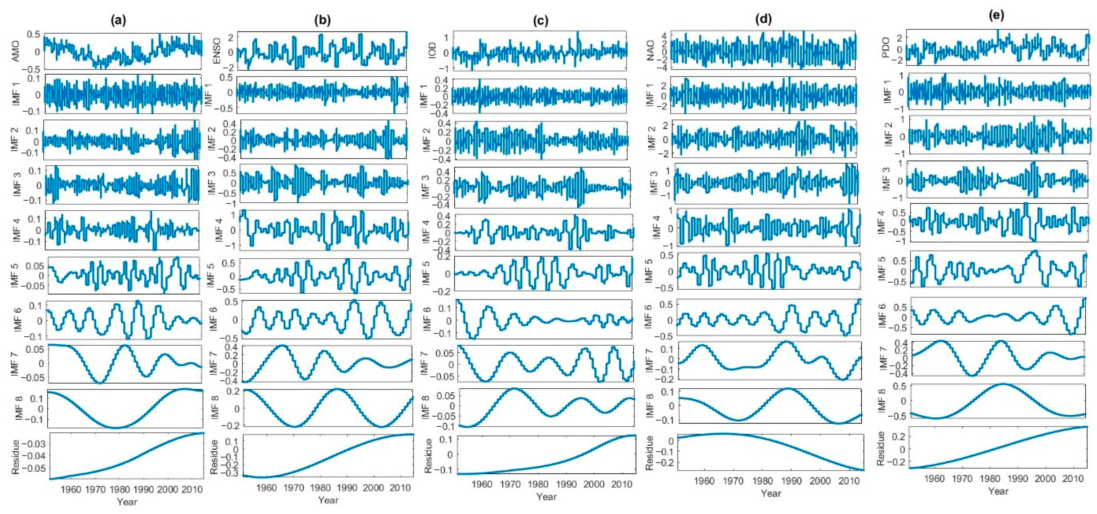
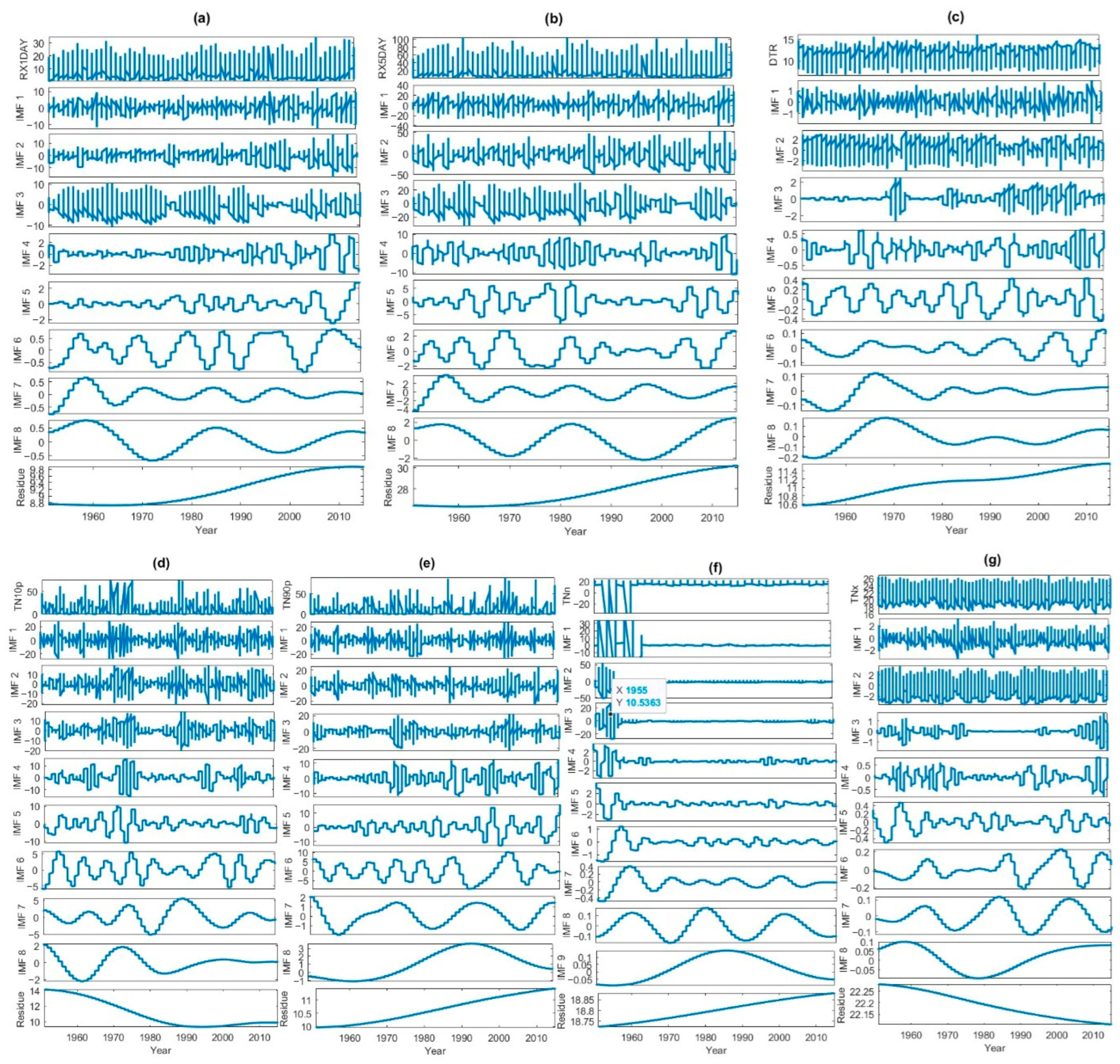
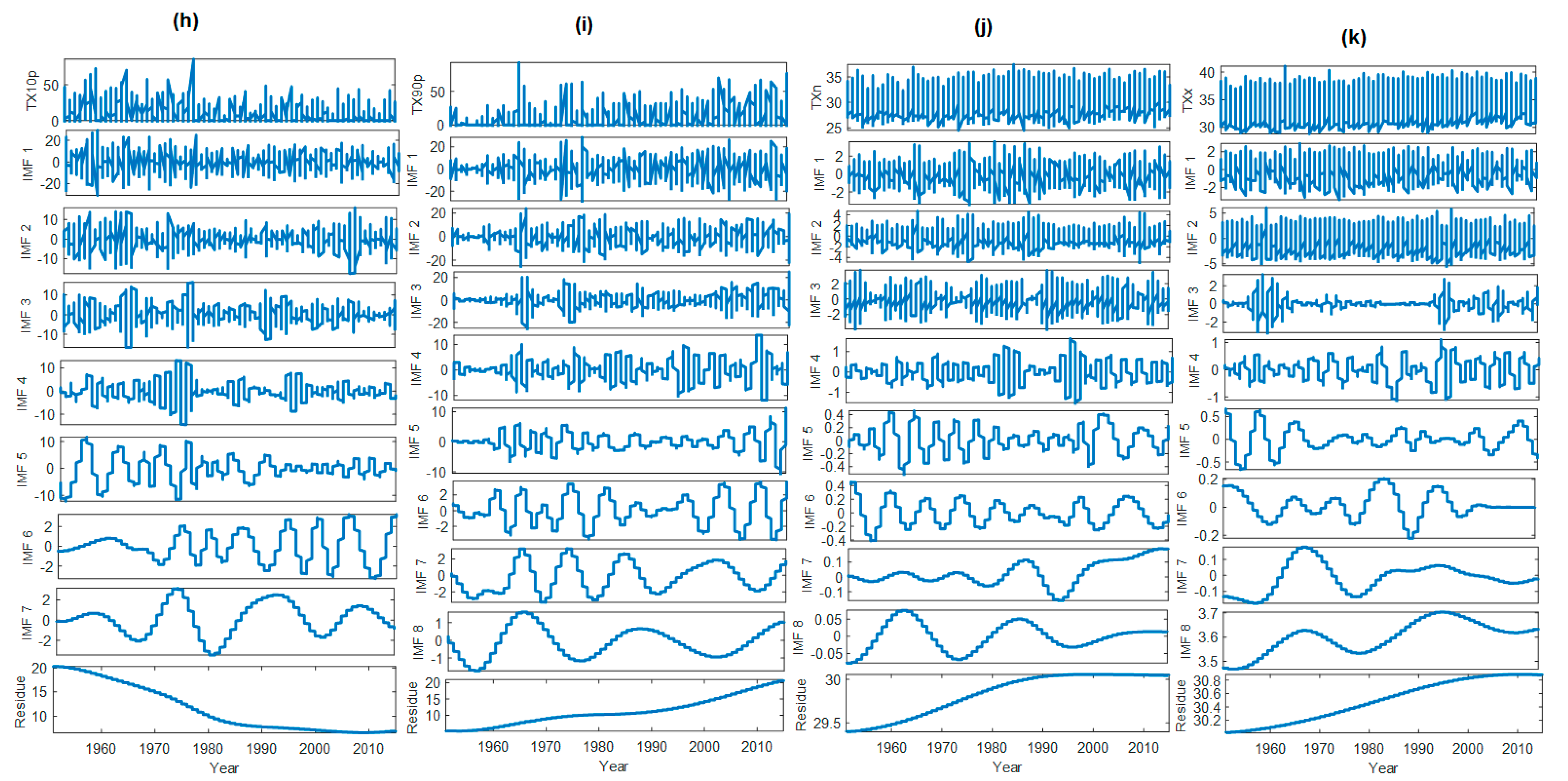
The monthly indices considered were the TN 90p, TN10p, TX 90p, TX 10, DTR, RX1Day, RX5Day, TXx, TNn, TXn, and TNx, and the climatic oscillations considered were the AMO, ENSO, IOD, NAO, and PDO. The IMF plot of the monthly indices and the climatic oscillations obtained by the CEEMDAN analysis for the SPI region are shown in Figure 5 and Figure 6.

Figure 6 shows that all the monthly indices and the climatic oscillations have different numbers of IMFs. The decomposition of all five climatic oscillations resulted in eight IMFs and residue. For the monthly indices, the DTR, Rx1 Day, TN90p, TN10p, TX90p, TXn, and TXx had eight IMFs, while Rx5Day and TNn had nine IMFs, and Tnx and TX10p had seven IMFs each. After obtaining the IMFs corresponding to the data signal for all the selected indices and oscillations, the significance of each plot was analyzed with a significance plot (Figure 7). In the significance plot, the IMFs above the red line showed a significance above 99%, and IMFs above the blue line showed a significance above 95%. The significance plot of all the indices of the SPI region is shown in Figure 7. For instance, for TN10p, except IMF 8, all other IMFs showed a significance above 99%, and in the case of climatic oscillations, a majority of oscillations showed a significance above 99%.

Once the significance was analyzed, the correlation of the signal with the data was analyzed, and it was found that for the indices Rx1Day, Rx5 Day, TN90p, TNn, TNx, and TXn, DTR, the second IMF showed a greater correlation with the signal, while for TX90p, TXx, TN10p, and TX10p, IMF 1 showed a greater correlation with the signal. The correlation values obtained are listed in

Table 2. The correlation values of all the indices used in this study.

Index	IMF1	IMF 2	IMF 3	IMF 4	IMF 5	IMF 6	IMF7	IMF8/ Residue	IMF9/ Residue	IMF 10/ Residue
RX1Day	0.446	0.614	0.585	0.067	0.057	0.055	0.068	0.044	0.031
RX5Day	0.363	0.680	0.535	0.0588	0.0504	0.0318	0.0619	0.003	−0.001	0.04
TN90p	0.452	0.498	0.467	0.355	0.339	0.273	0.0562	0.066	0.105
TNn	0.309	0.459	0.233	0.154	0.083	0.118	0.120	0.054	0.078	0.085
TNx	0.48	0.851	0.127	0.063	0.041	0.0357	0.0154	0.01357
TX90p	0.520	0.398	0.486	0.376	0.298	0.212	0.164	0.121	0.312	0.294
TXn	0.406	0.671	0.613	0.091	0.066	0.077	0.022	0.031	0.096
TXx	0.520	0.398	0.485	0.376	0.297	0.212	0.163	0.121	0.312	0.294
DTR	0.377	0.844	0.303	0.067	0.049	0.048	0.091	0.071	0.118
TN10p	0.533	0.419	0.394	0.332	0.270	0.143	0.116	0.064	0.048
TX10p	0.606	0.349	0.350	0.289	0.301	0.090	0.048	0.304

.

Regarding TX90P, a value of 0.52 indicates a moderate positive linear relationship (on a scale from −1 to 1), meaning that about 27% (0.52²) of the variance in TX90p IMF1 is explained by the corresponding IMFs from COs. This is not extremely strong but is statistically notable in climate contexts, where signals are often noisy. IMF1 represents the highest frequency variability (short-term fluctuations, e.g., intra-seasonal or weather-scale noise, often on timescales of weeks to months). Therefore, it is concluded that COs primarily influence heat-related extremes through high-frequency, short-term processes. This could imply that the rapid atmospheric teleconnections driven by these indices are most evident in TX90p’s fast-varying components. In addition, the short-term variability in TX90p, such as sudden heatwaves, may be more synchronized with the quick oscillations.

Regarding precipitation extremes (Rx1Day and Rx5Day), the shift in the maximum correlation to IMF2 indicates that extreme rainfall events are more strongly linked to slightly lower-frequency components of COs. This suggests influences operating on seasonal to inter-annual timescales, where processes like atmospheric moisture transport, storm track shifts, or monsoon modulations (driven by COs) accumulate to affect heavy precipitation.

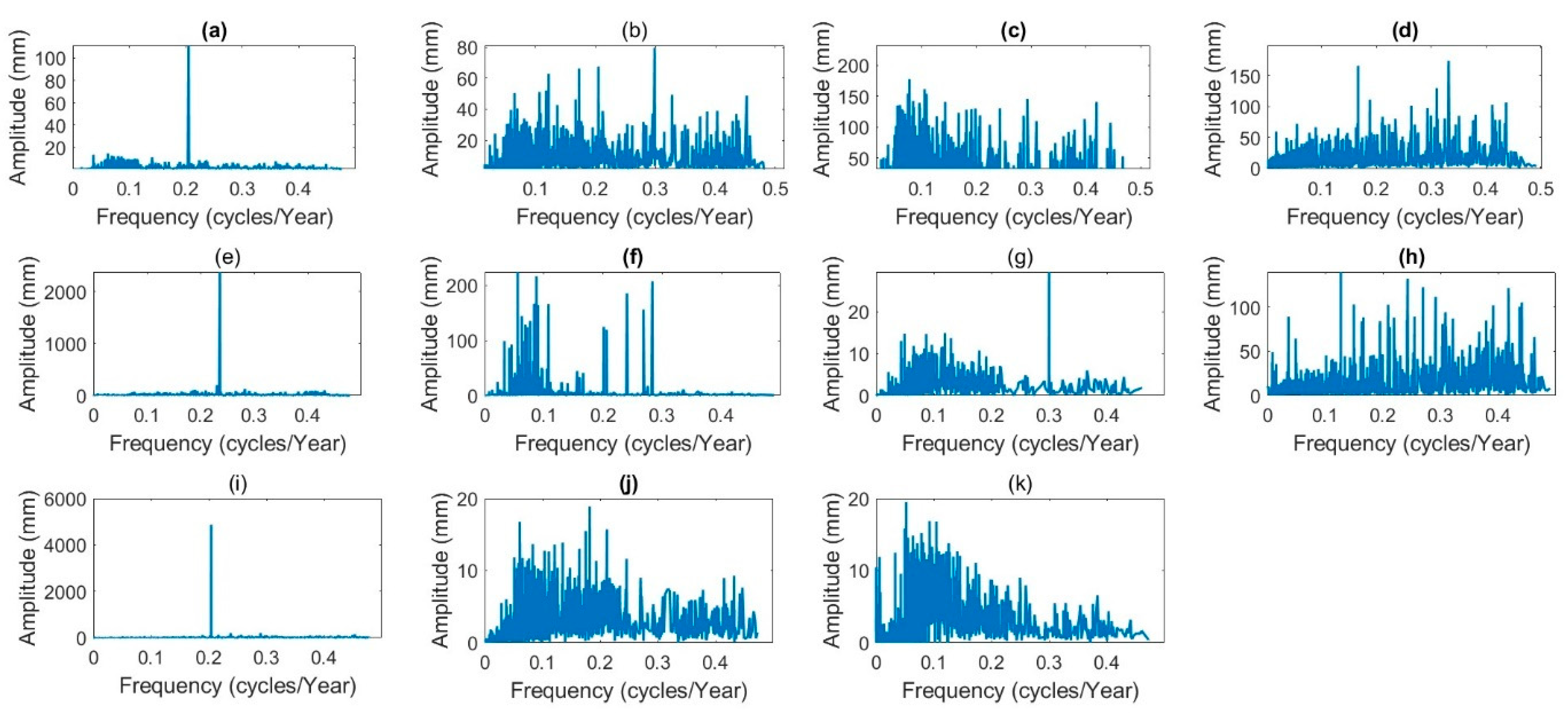
A marginal Hilbert spectrum (frequency amplitude plot) of the indices was also developed and is presented in Figure 8. The frequency–amplitude plots show a unique prominent spike for DTRm TN90p, TX90p, and TNx, but multiple prominent frequencies are exhibited in the marginal Hilbert spectrum of the indices.

The periods of all the IMFs were computed using the zero-crossing method [44], which is consolidated into a tabular form in

Table 3. Table showing the periodicity values of all the indices.

Index	IMF
	1	2	3	4	5	6	7	8 Residue	9 Residue
RX1	3.158	7.156	13	24.38	52	97.5	156	260	780
RX5	3.49	7.96	13.93	26	48.75	86.67	195	260	390
TN90p	3.12	6.29	11.64	21.08	41.05	86.67	156	780
TNn	3.64	10.68	12.19	20	41.05	70.91	130	260	780
TNx	4.51	11.14	11.64	26.90	65	195	390	780
TX90p	3.25	6.046	11.64	21.08	37.14	65	111.429	260	780
TXn	3.35	7.22	13	24.38	48.75	78	156	260	780
TXx	3.88	10.99	17.33	32.5	70.91	78	390	780
DTR	3.18	9.63	17.33	25.16	65	111.43	195	260
TN10p	3.07	5.95	11.82	23.64	45.88	86.67	156	260	780
TX10p	3.07	5.95	11.82	23.64	45.8824	86.67	156	260	780

. The periodic scales are non-dyadic in nature, as expected, which is a typical characteristic of the HHT and is helpful in proceeding with the running correlation analysis.

4.3. Correlation Analysis

This study’s major objective lies in estimating the correlation between climatic indices and COs. The useful statistical method of the correlation analysis makes understanding the relationship between variables possible. Here three types of analyses are performed.

Linear Correlation

The linear association between indices and oscillations is determined using simple Pearson correlations. The linear correlation values calculated are consolidated into a tabular form and are shown in

Table 4. Correlation coefficient (CC) values of SPI region.

Oscillation	Indices	CC	Oscillation	Indices	R
AMO	RX1	0.112	NAO	RX1	−0.044
	RX5	0.105		RX5	−0.048
	DTR	−0.114		DTR	0.060
	TN10p	−0.089		TN10p	0.006
	TN90p	0.096		TN90p	0.034
	TNn	−0.023		TNn	−0.034
	TNx	0.093		TNx	−0.084
	TX10p	−0.068		TX10p	0.070
	TX90p	0.024		TX90p	−0.003
	TXn	0.029		TXn	−0.044
	TXx	0.027		TXx	−0.055
ENSO	RX1	0.017	PDO	RX1	−0.794
	RX5	−0.016		RX5	0.950
	DTR	0.023		DTR	0.033
	TN10p	−0.241		TN10p	−0.017
	TN90p	0.237		TN90p	0.017
	TNn	0.015		TNn	0.185
	TNx	0.012		TNx	0.149
	TX10p	−0.270		TX10p	0.074
	TX90p	0.222		TX90p	−0.086
	TXn	0.066		TXn	−0.390
	TXx	0.037		TXx	0.179
IOD	RX1	−0.077
	RX5	−0.091
	DTR	0.159
	TN10p	−0.034
	TN90p	0.148
	TNn	−0.037
	TNx	−0.040
	TX10p	−0.149
	TX90p	0.169
	TXn	0.076
	TXx	0.048

.

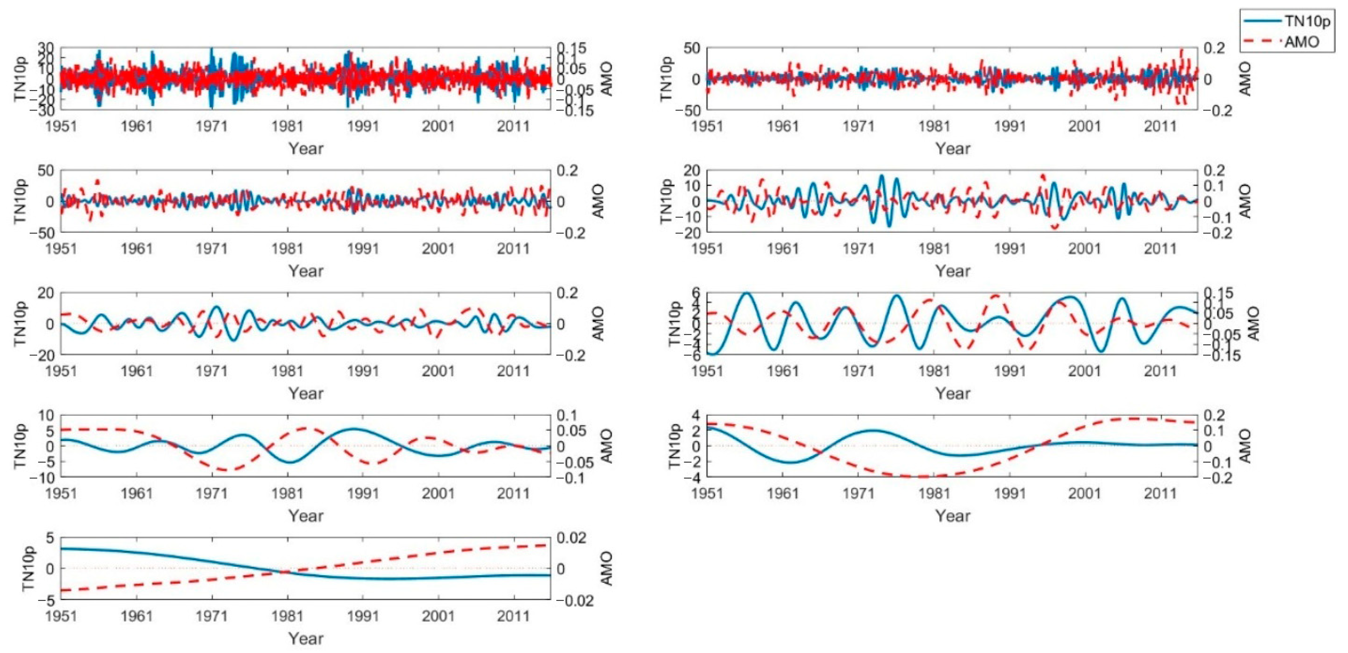
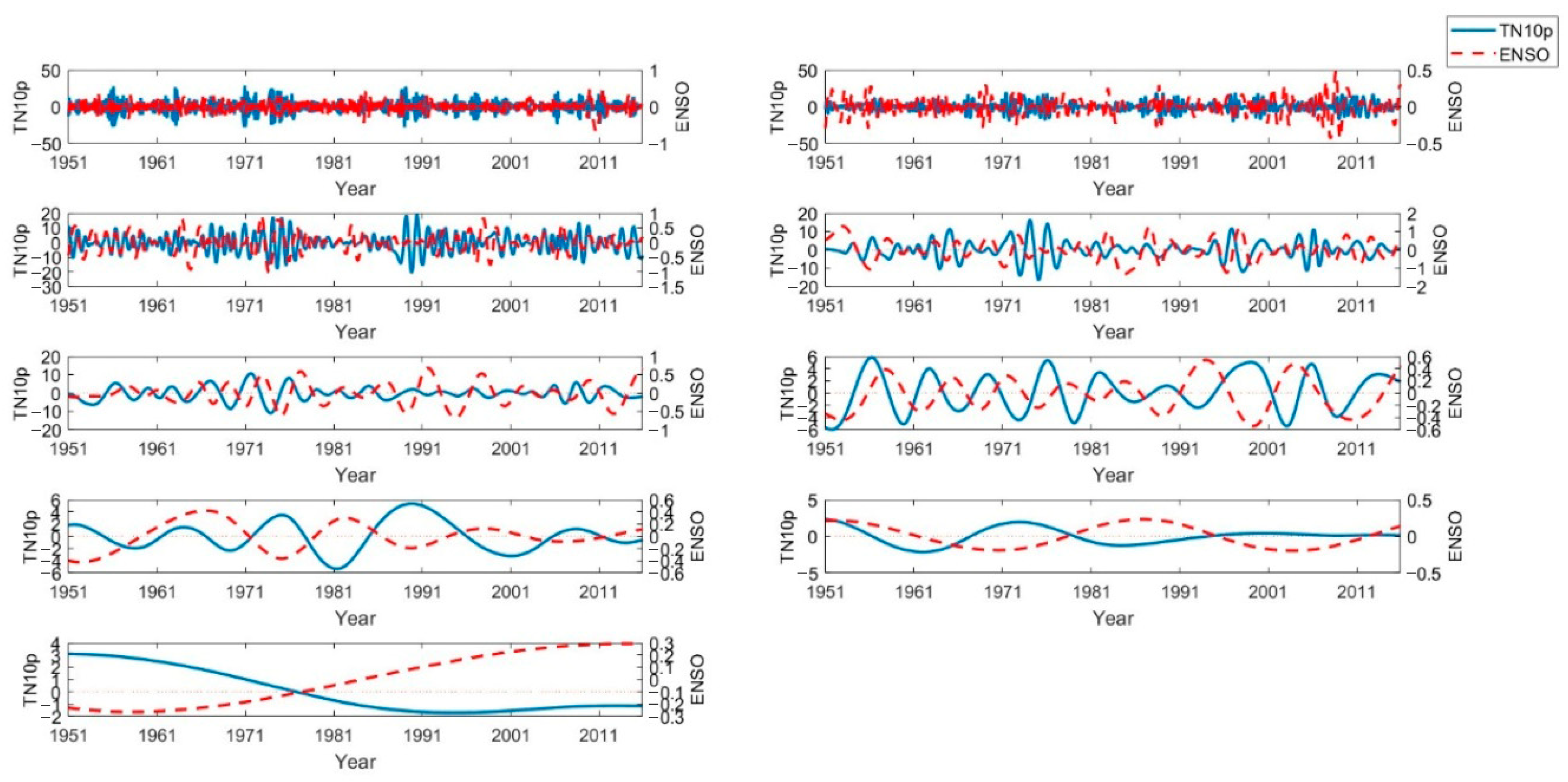
Table 4 clearly indicates that the linear association between COs and ECIs is very weak, which is expected in a multiscale nonlinear process. Moreover, time-lagged information is not specifically considered by Pearson’s correlation. In multiscale processes, a conventional correlation analysis of the time series alone cannot fully capture the associations between COs and hydrologic or meteorological variables. To reveal scale-specific relationships between COs and ECIs, we generated comparison plots of corresponding IMFs and residuals. Lead–lag relationships become evident when examining the correlations between the indices and oscillations, as illustrated in Figure 9 and Figure 10.

The correlation values obtained from all the IMFs of the AMO and TN10p were analyzed, as shown in

Table 5. Table showing the correlation values of IMFs of AMO and TN10p. Significant correlations are marked in bold text.

	AMO	1	2	3	4	5	6	7	8	Residue
TN10P
1		0.072	−0.011	0.017	−0.01	−0.013	−0.006	0.019	−0.011	0.007
2		−0.026	0.109	0.041	−0.047	−0.039	−0.008	−0.002	−0.009	−0.004
3		0.026	0.032	−0.048	−0.125	0.012	0.023	−0.005	0.001	−0.002
4		−0.015	−0.008	−0.016	−0.124	−0.054	−0.054	−0.015	−0.024	−0.001
5		−0.005	0.002	−0.007	−0.155	−0.432	−0.056	0.05	0.088	0.012
6		0.017	0.009	−0.015	−0.067	−0.071	0.126	−0.212	−0.064	0.022
7		−0.027	0.002	0.042	−0.036	−0.065	0.035	−0.425	−0.469	0.356
8		−0.018	0.008	0.023	−0.021	−0.052	0.042	−0.124	0.06	0.074
9		0.041	0.003	−0.021	−0.009	0.048	0.161	−0.037	0.017	−0.878

. Similarly, correlation values obtained from all the IMFs of the ENSO and TN90p were analyzed, as shown in

Table 6. Table showing the correlation values of IMFs of ENSO and TN10p. Significant correlations are marked in bold text.

	ENSO	1	2	3	4	5	6	7	8	Residue
TN10P
1		0.031	−0.064	0.049	−0.018	0.003	−0.008	0.016	0.001	0.026
2		−0.007	0.008	0.124	−0.029	−0.003	0.009	0.006	0.007	−0.001
3		0.007	0.001	0.016	−0.406	−0.002	0.02	−0.009	0.039	0.003
4		0.012	−0.005	−0.039	−0.211	−0.42	−0.187	0.096	0.163	0.162
5		−0.012	0.001	−0.001	−0.078	−0.241	−0.052	−0.007	−0.005	−0.025
6		−0.01	−0.01	−0.022	0.051	0.139	−0.182	−0.075	−0.141	−0.089
7		0.013	−0.006	0.004	0.012	0.114	0.138	−0.487	−0.561	−0.092
8		−0.004	−0.002	−0.037	−0.029	−0.109	−0.041	0.238	−0.303	0.096
9		0.042	0.003	−0.018	−0.013	0.034	0.147	−0.016	0.045	−0.886

.

Figure 9 and Figure 10 clearly exhibit the lead–lag relationship between the two variables. In the lower mode IMFs, both the variables show similar patterns, and no lead–lag is seen there. But as the higher mode is correlated, both the variables show different patterns, and a lead–lag relation is established, and in certain higher mode IMFs, a strong positive correlation was seen. The p-value obtained during the correlation analysis indicates the likelihood that a correlation coefficient as extreme as the reported one would occur. In other words, it measures how likely it is that the observed correlation coefficient would be obtained even in the absence of a relationship between the variables. Significance values (≤(+/−)0.5) were noted and are marked in the table. But with climatic data being non-stationary and nonlinear, only very few IMFs showed significant correlations, making the linear correlation process unsuitable for further studies and thereby the correlation analysis of the hydroclimatic data. Moreover, the window period is fixed, meaning that the correlation results may be inaccurate. Thus, an improved approach for the TDIC was used for our study.

The TDIC is an HHT-based running correlation analysis technique, designed to analyze and capture the local correlation between non-stationary and nonlinear series pairs. The TDIC is a more dynamic and sophisticated notion than traditional correlations. It uses IMFs to determine a set of sliding window sizes for the computation of the correlation for multiscale data. The selection of sliding windows is an adaptive data-dependent process, thus making the process more credible for the study of climatic indices and oscillations. A TDIC analysis was performed for all the selected indices and oscillations. The main advantage of this method is that it can produce a better understanding of how each IMF is correlated.

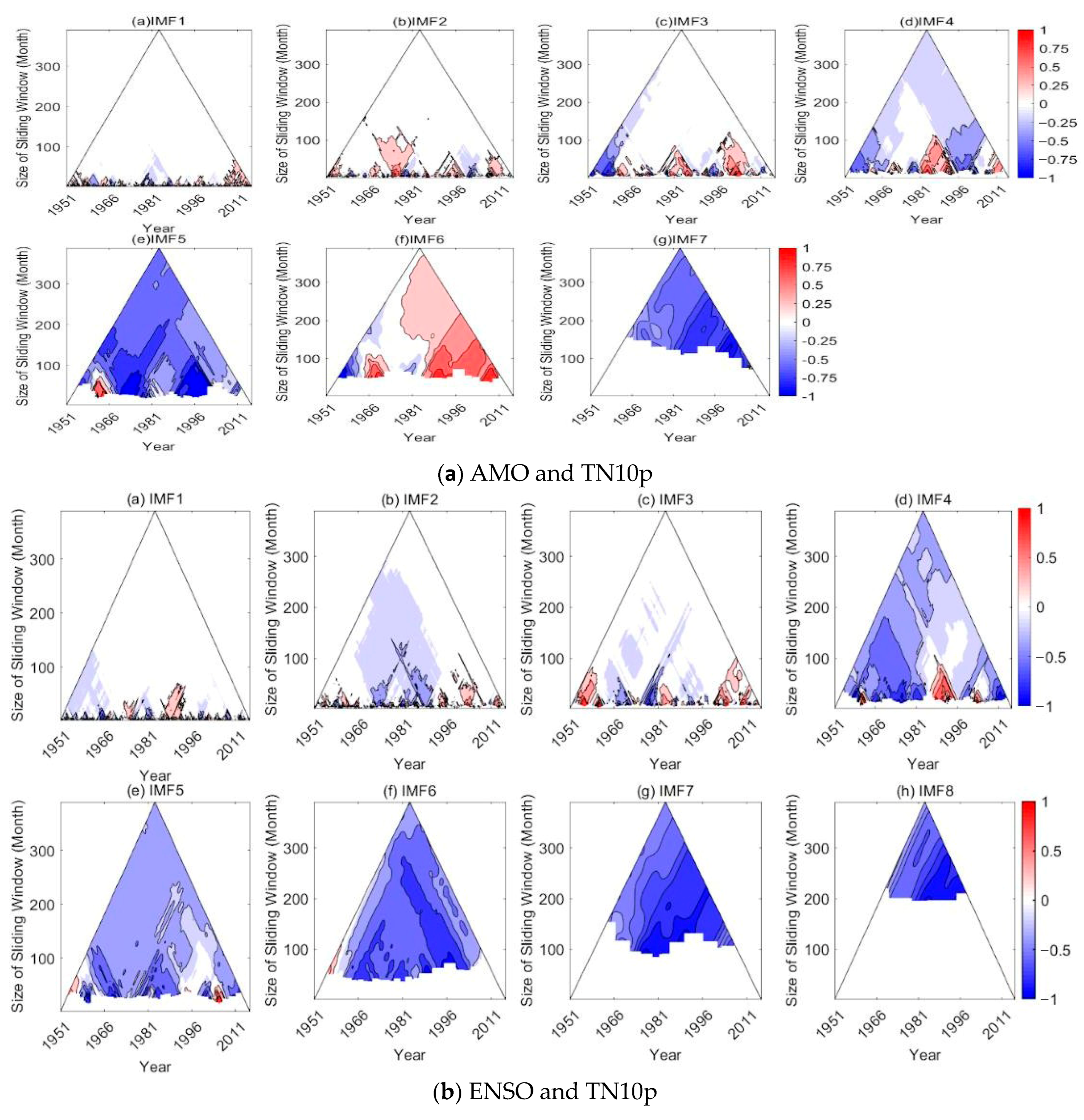
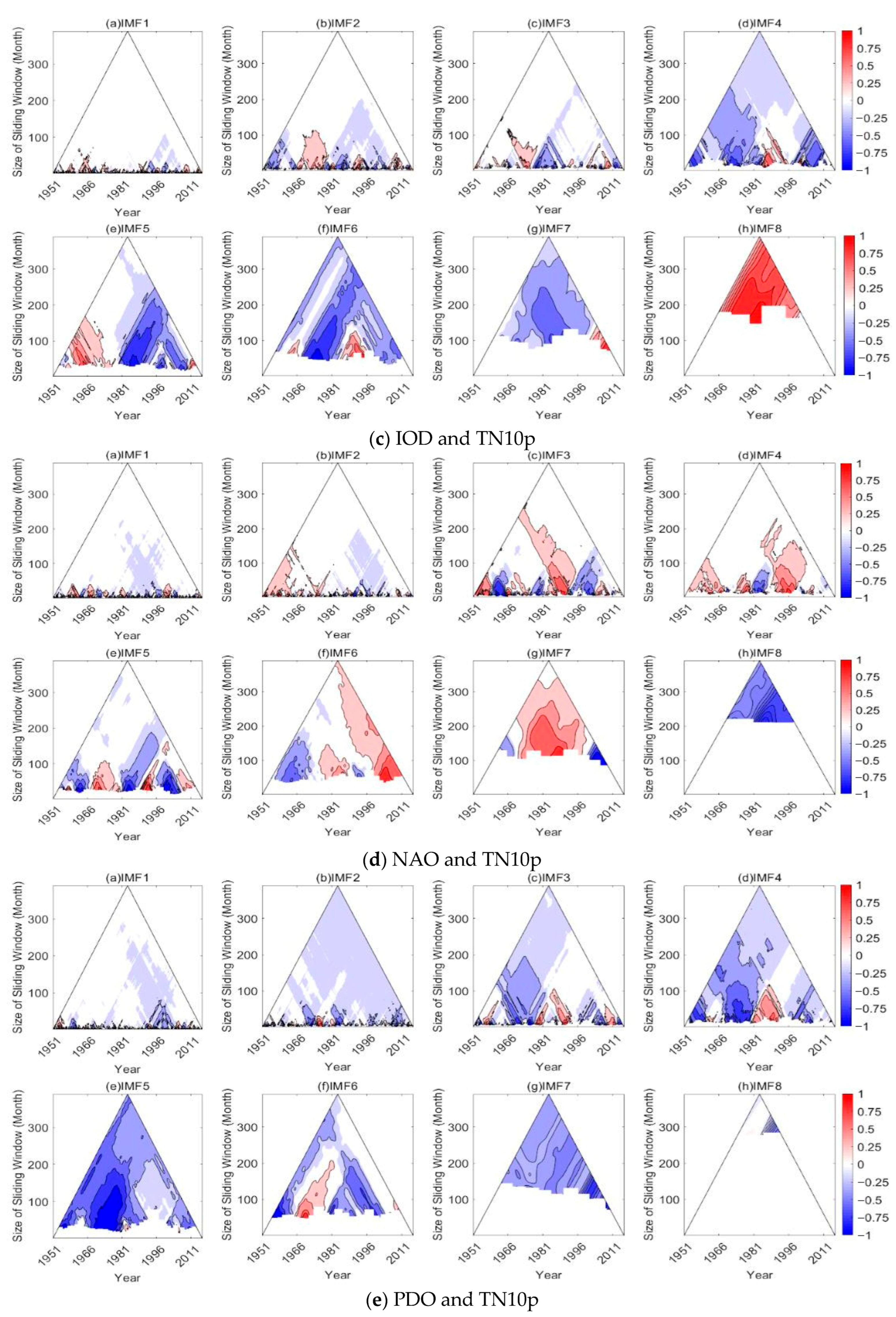
The TDIC analysis of the SPI region for all five climatic oscillations and TN10p is shown in Figure 11. The red regions showed a positive correlation, while the blue regions showed a negative correlation.

From Figure 10 and Figure 11, all the lower mode IMFs have many voids, which indicate that those spaces have failed to satisfy Students’ test, hence making them highly insignificant for further modeling [34,35]. In case of the correlation of the AMO, ENSO, IOD, and PDO with TN10p, the majority of IMFs showed negative correlations, and we can say that the effect of cool nights in the SPI region due to the AMO, ENSO, IOD and PDO is smaller. But for same index when associated with the NAO, IMFs showed more positive correlations when compared to other oscillations. The AMO in SPI has notable effects for the indices Rx1Day, Rx5Day, TNn, and TNx, while all other indices have no notable effect when analyzing the correlation. When associated with the AMO, IMF 7 of TN10p showed a strong negative correlation, which indicates that it can be used for future modeling since the concerned IMF shows a significance of more than 99%. The ENSO-TN10p relationship is strongly positive for IMF7, while it is strongly negative for TX10p. In relation to the PDO, TX10p and TN10p have the possibility of showing notable effects. The relations with the IOD are inconsistent in nature (transitions from positive to negative and vice versa) along the time domain in different IMFs. In association with the IOD, the DTR and TXx may have notable effects since their corresponding IMFs show more positive correlations when compared to negative correlations. When related to the NAO, the TNn shows an overall negative correlation. IMF5 of the TN10p and TX10p; IMF 6 of TN90p; and IMF 4, 5, and 7 of TX10p showed strong negative correlations with the PDO in the SPI region. IMF 7 of the TNx showed a strong positive correlation for the PDO in PI. In short, we can conclude that while analyzing the correlations of climatic oscillations and extreme climatic indices of PI, the climatic PDO and IOD must be given more importance.

This study computed the long-range correlation between ECIs and COs at different time scales to identify the ECI-CO dynamics and the corresponding time scales. By identifying the relevant IMFs of each signal and identifying the specific COs modulating ECIs that are significant in a particular region, we can develop predictive models by integrating the TDIC with machine learning tools [35]. This could be supportive for tracking the future changes in extreme temperatures and precipitation, allowing for early planning and mitigation.

This study presented a novel improved HHT-based TDIC approach for investigating the teleconnections of ECIs with climatic oscillations. In the traditional spectral analysis method, the scale-specific information of the dominant frequency cannot be captured, while the hydroclimatic processes, like extreme indices, are multiscale in nature and hence demand the capture of such information to develop effective predictive models. Here the dominant frequency of each mode can be captured by a Hilbert spectral analysis of decomposed modes. Moreover, the dominant modes in each predictor set can be identified and retained for developing predictive models of extreme indices, as illustrated in the workflow of the MEMD-SLR models [35]. The time-lagged information is crucial for developing such predictive models, which can be fixed by optimizing the inputs by the TDIC plots, as illustrated [36]. The traditional correlation between the signals of ECIs and COs may be very low, as the positive correlation between the two at some specific process scale may get neutralized by the negative correlation in some other scale. To deal with such multiscale associations, the TDIC is an alternative and powerful approach, as it accounts for the non-stationarity of the datasets while performing a dynamic correlation analysis. However, this study is to be extended to quantify the association in a cross-correlation framework, considering the modes across different process scales. Along with the TDIC matrix, ASC measures across different scales [45] need to be quantified to extend the present framework for the prediction of extreme climatic indices. Along with the statistical analysis using the HHT and TDIC, the physical processes governing the transition of correlations (from positive to negative and vice versa) along the time domain are to be assessed by ground truth exercises in relation to different episodes of extremes in the respective geographical regions. For such a case, the role of the local-scale meteorology and the concurrent effect of multiple oscillations are to be investigated in detail for sound physical interpretations. In such an exercise, a comprehensive analysis of the physical mechanisms behind rainfall, clouds, atmospheric rivers, etc., using remote sensing and GIS techniques may also be helpful [46,47,48]. Hence, a combination of physics-based modeling, geospatial modeling, and advanced spectral analysis tools, like the HHT-based TDIC, can provide a better understanding of hydroclimate dynamics and helpful inputs for improved predictions of climate extremes.

Although the proposed CEEMDAN–TDIC framework provides a flexible and data-driven approach for detecting time- and frequency-localized teleconnections, several limitations should be noted. First, many correlations identified at the IMF level, particularly in higher-frequency modes, do not reach statistical significance, resulting in large areas of non-significant associations. This reduces the robustness of some reported oscillation–extreme linkages and highlights the challenge of distinguishing physically meaningful signals from noise in decomposed components. Second, the use of spatially averaged ETCCDI indices across SPI may mask important sub-regional variability, especially given the sharp climatic gradients induced by the Western Ghats, the rain shadow effect over the Deccan Plateau, and the contrasting exposure of western and eastern coastal zones. Third, while the TDIC effectively captures non-stationary and nonlinear relationships, the findings have not yet been cross-validated against complementary methods, such as wavelet coherence analysis or physically based monsoon indices. Future work will therefore focus on (i) applying more stringent significance testing and false discovery rate controls across IMFs, (ii) conducting the analysis at a higher spatial resolution (e.g., homogeneous sub-regional level), and (iii) systematically comparing CEEMDAN–TDIC results with alternative teleconnection diagnostics to strengthen confidence in the identified multiscale oscillation–extreme relationships.

5. Conclusions

This research examined the possible relation between the five selected COs, namely the ENSO, AMO, NAO, PDO, and IOD, with the monthly ECOs defined by ETCCDI over Peninsular India in a running correlation approach. In general, the relation between climatic oscillations and ECOs is found to be dynamic in nature, both in the time scale and time domain. The low-frequency scales have consistent relations with extremes, while at high-frequency scales, we found that the nature of the association displayed a transition along the time domain because of the effects of multiple oscillations and local meteorological variables at specific times. The other specific findings of this study include the following:

• The PDO and AMO decrease the chance of cool nights in the SPI region, while no oscillations considered in this study increase the occurrence of low-temperature nights in SPI.
• The AMO diminishes the chances of achieving the maximum highest daily temperature.
• The NAO reduces the daily maximum temperature of SPI, while the ENSO increases the chances for one-day maximum rainfall in SPI.
• Overall, we concluded that the PDO and IOD must be given more importance when analyzing the correlations of climatic oscillations and ECOs across SPI.
• High-frequency IMFs (IMF1-3) showed variegated correlations and are downplayed by the presence of voids.

Conclusively, these efforts will facilitate further studies related to climatic variabilities and their correlation with climatic oscillations and the modeling of better climatic predictions.

References

1. Yan, Z.; Yang, J.; Zhang, H.; Li, W.; Wang, Y.; Liu, H.; Yu, L. Biophysical feedback from earlier leaf-out enhances nonerosive precipitation in China. Commun. Earth Environ. 2025. [Google Scholar] [CrossRef]
2. Chai, Y.; Miao, C.; Gentine, P.; Mudryk, L.; Thackeray, C.W.; Berghuijs, W.R.; Wu, Y.; Fan, X.; Slater, L.; Sun, Q.; et al. Constrained Earth system models show a stronger reduction in future Northern Hemisphere snowmelt water. Nat. Clim. Change 2025, 15, 514–520. [Google Scholar] [CrossRef]
3. Chen, X.; Dai, A. Quantifying contributions of external forcing and internal variability to Arctic warming during 1900–2021. Earth’s Future 2024, 12, e2023EF003734. [Google Scholar] [CrossRef]
4. Gayathri, M.S.; Adarsh, S.; Shehinamol, K.; Nizamudeen, Z.; Lal, M.R. Evaluation of change points and persistence of extreme climatic indices across India. Nat. Hazards 2023, 116, 2747–2759. [Google Scholar] [CrossRef]
5. Zhang, X.; Alexander, L.; Hegerl, G.C.; Jones, P.; Tank, A.K.; Peterson, T.C.; Trewin, B.; Zwiers, F.W. Indices for monitoring changes in extremes based on daily temperature and precipitation data. Wiley Interdiscip. Rev.-Clim. Change 2011, 2, 851–870. [Google Scholar] [CrossRef]
6. Roy, S.S.; Balling, R.C., Jr. Trends in extreme daily precipitation indices in India. Int. J. Climatol. 2004, 24, 457–466. [Google Scholar] [CrossRef]
7. Aguilar, E.; Peterson, T.C.; Obando, P.R.; Frutos, R.; Retana, J.A.; Solera, M.; Soley, J.; García, I.G.; Araujo, R.M.; Santos, A.R.; et al. Changes in precipitation and temperature extremes in Central America and northern South America, 1961–2003. J. Geophys. Res. 2005, 110, D23107. [Google Scholar] [CrossRef]
8. Yin, H.; Sun, Y. Characteristics of extreme temperature and precipitation in China in 2017 based on ETCCDI indices. Adv. Clim. Change Res. 2018, 9, 218–226. [Google Scholar] [CrossRef]
9. Yosef, Y.; Aguilar, E.; Alpert, P. Is it possible to fit extreme climate change indices together seamlessly in the era of accelerated warming. Int. J. Climatol. 2021, 41, E952–E963. [Google Scholar] [CrossRef]
10. Modaresi, F.; Danandeh Mehr, A.; Bajgiran, I.S.; Safari, M.J.S. Multi-level trend analysis of extreme climate indices by a novel hybrid method of fuzzy logic and innovative trend analysis. Sci. Rep. 2025, 15, 27432. [Google Scholar] [CrossRef]
11. Sankaran, A.; Madhusudanan, S.G.; Ndehedehe, C.; Nair, A.N.G.R. Spatio-temporal Variability of Trends in Extreme Climatic Indices across India. KSCE J. Civil. Eng. 2024, 28, 2537–2551. [Google Scholar] [CrossRef]
12. Sankaran, A.; Ahmed, A.N.; Elshafie, A.N.; Sherif, M.; Antony, A.M.; Anilkumar, K.; Raheena, L.N.; Purath, J.T. Deciphering the teleconnections of Extreme Temperature Indices with Local scale Meteorology using wavelet coherence. Phys. Chem. Earth 2025, 140, 104009. [Google Scholar] [CrossRef]
13. Gadgil, S.; Vinayachandran, P.N.; Francis, P.A.; Gadgil, S. Extremes of the Indian summer monsoon rainfall, ENSO and equatorial Indian Ocean oscillation. Geophys. Res. Lett. 2004, 31, L12213. [Google Scholar] [CrossRef]
14. Sankaran, A.; Reddy, M.J. Analyzing the Hydroclimatic Teleconnections of Summer Monsoon Rainfall in Kerala, India, Using Multivariate Empirical Mode Decomposition and Time-Dependent Intrinsic Correlation. IEEE Geosci. Remote Sens. Lett. 2016, 13, 1221–1225. [Google Scholar] [CrossRef]
15. Adarsh, S.; Reddy, M.J. Links between global climate teleconnections and Indian monsoon rainfall. In Climate Change Signals and Response: A Strategic Knowledge Compendium for India; Springer: Singapore, 2018; pp. 61–72. [Google Scholar]
16. Mohammadi, B.; Vaheddoost, B.; Mehr, A.D. A spatiotemporal teleconnection study between Peruvian precipitation and oceanic oscillations. Quat. Int. 2020, 565, 1–11. [Google Scholar] [CrossRef]
17. Torrence, C.; Compo, G.P. A practical guide to wavelet analysis. Bull. Am. Meteorol. Soc. 1998, 79, 61–78. [Google Scholar] [CrossRef]
18. Zhang, L.; Su, H.; Zio, E.; Zhang, Z.; Chi, L.; Fan, L.; Zhou, J.; Zhang, J. A data-driven approach to anomaly detection and vulnerability dynamic analysis for large-scale integrated energy systems. Energy Convers. Manag. 2021, 234, 113926. [Google Scholar]
19. Kurths, J.; Agarwal, A.; Shukla, R.; Marwan, N.; Rathinasamy, M.; Caesar, L.; Krishnan, R.; Merz, B. Unravelling the spatial diversity of Indian precipitation teleconnections via a non-linear multi-scale approach. Nonlin. Proc. Geophys. 2019, 26, 251–266. [Google Scholar]
20. Rathinasamy, M.; Agarwal, A.; Sivakumar, B.; Marwan, N.; Kurths, J. Wavelet analysis of precipitation extremes over India and teleconnections to climate indices. Stoch. Environ. Res. Risk Assess. 2019, 33, 2053–2069. [Google Scholar] [CrossRef]
21. Kalyan, A.V.S.; Ghose, D.K.; Thalagapu, R.; Guntu, R.K.; Agarwal, A.; Kurths, J.; Rathinasamy, M. Multiscale spatiotemporal analysis of extreme events in the Gomati River Basin, India. Atmosphere 2021, 12, 480. [Google Scholar] [CrossRef]
22. Nourani, V.; Tootoonchi, R.; Andaryani, S. Investigation of climate, land cover and lake level pattern changes and interactions using remotely sensed data and wavelet analysis. Ecol. Inform. 2021, 64, 101330. [Google Scholar] [CrossRef]
23. Mohan, M.G.; Fathima, S.; Adarsh, S.; Baiju, N.; Nair, G.A.; Meenakshi, S.; Krishnan, M.S. Analyzing the streamflow teleconnections of greater Pampa basin, Kerala, India using wavelet coherence. Phys. Chem. Earth 2023, 131, 103446. [Google Scholar] [CrossRef]
24. Su, H.; Zio, E.; Zhang, J.; Xu, M.; Li, X.; Zhang, Z. A hybrid hourly natural gas demand forecasting method based on the integration of wavelet transform and enhanced Deep-RNN model. Energy 2019, 178, 585–597. [Google Scholar] [CrossRef]
25. Huang, N.E.; Shen, Z.; Long, S.R.; Wu, M.C.; Shih, H.H.; Zheng, Q.; Yen, N.-C.; Chao, C.; Tung, C.C.; Liu, H.H. The empirical mode decomposition and the Hilbert spectrum for nonlinear and non-stationary time series analysis. Proc. R. Soc. London Ser. A Math. Phys. Eng. Sci. 1998, 454, 903–995. [Google Scholar] [CrossRef]
26. Someetheram, V.; Marsani, M.F.; Kasihmuddin, M.S.M.; Jamaludin, S.Z.M.; Mansor, M.A.; Zamri, N.E. Hybrid double ensemble empirical mode decomposition and K-Nearest Neighbors model with improved particle swarm optimization for water level forecasting. Alex. Eng. J. 2025, 115, 423–433. [Google Scholar] [CrossRef]
27. Wu, Z.; Huang, N.E. Ensemble empirical mode decomposition: A noise-assisted data analysis method. Adv. Adapt. Data Anal. 2009, 1, 1–41. [Google Scholar] [CrossRef]
28. Torres, M.E.; Colominas, M.A.; Schlotthauer, G.; Flandrin, P. A complete ensemble empirical mode decomposition with adaptive noise. In Proceedings of the 2011 IEEE International Conference on Acoustics, Speech and Signal Processing (ICASSP), Prague, Czech Republic, 22–27 May 2011; pp. 4144–4147. [Google Scholar]
29. Colominas, M.A.; Schlotthauer, G.; Torres, M.E. Improved complete ensemble EMD: A suitable tool for biomedical signal processing. Biomed. Signal Process. Control 2014, 14, 19–29. [Google Scholar] [CrossRef]
30. Adarsh, S.; Plocoste, T.; Nourani, V. Application of Hilbert Huang Transform Framework for Characterizing the Multiscale Properties of Air Temperature in India over a Century. Pure Appl. Geophys. 2025, 182, 3341–3371. [Google Scholar] [CrossRef]
31. Chen, X.; Wu, Z.; Huang, N.E. The time-dependent intrinsic correlation based on the empirical mode decomposition. Adv. Adapt. Data Anal. 2010, 2, 233–265. [Google Scholar] [CrossRef]
32. Huang, Y.; Schmitt, F.G. Time dependent intrinsic correlation analysis of temperature and dissolved oxygen time series using empirical mode decomposition. J. Mar. Syst. 2014, 130, 90–100. [Google Scholar] [CrossRef]
33. Ashwini, K.; Pulak, G.; Savita, P.; Sulochana, G. Meteorological sub-divisions of India: Assessment of coherence, homogeneity and recommended redelineation. Mausam 2020, 71, 585–604. [Google Scholar] [CrossRef]
34. Adarsh, S.; Reddy, M.J. Multiscale characterization and prediction of monsoon rainfall in India using Hilbert–Huang transform and time-dependent intrinsic correlation analysis. Meteorol. Atmos. Phys. 2018, 130, 667–688. [Google Scholar]
35. Adarsh, S.; Janga Reddy, M. Multiscale characterization and prediction of reservoir inflows using MEMD-SLR coupled approach. J. Hydrol. Eng. 2019, 24, 04018059. [Google Scholar] [CrossRef]
36. Johny, K.; Pai, M.L.; Adarsh, S. Time-dependent intrinsic cross-correlation approach for multi-scale teleconnection analysis for monthly rainfall of India. Meteorol. Atmos. Phys. 2022, 134, 73. [Google Scholar] [CrossRef]
37. Gunnell, Y. Relief and climate in South Asia: The influence of the western ghats on the current climate pattern of peninsular India. Int. J. Climatol. 1998, 17, 1169–1182. [Google Scholar] [CrossRef]
38. Rilling, G.; Flandrin, P.; Gonçalves, P.; Lilly, J.M. Bivariate empirical mode decomposition. IEEE Signal Process. Lett. 2007, 14, 936–939. [Google Scholar] [CrossRef]
39. Rehman, N.; Mandic, D.P. Empirical mode decomposition for trivariate signals. IEEE Trans. Signal Process. 2009, 58, 1059–1068. [Google Scholar] [CrossRef]
40. Rehman, N.; Mandic, D.P. Multivariate empirical mode decomposition. Proc. R. Soc. A Math. Phys. Eng. Sci. 2010, 466, 1291–1302. [Google Scholar]
41. Yamuna, A.; Vyshnav, P.; Warrier, A.K.; Manoj, M.; Sandeep, K.; Kawsar, M.; Joju, G.; Sharma, R. Increasing frequency of extreme climatic events in southern India during the Late Holocene: Evidence from lake sediments. Quat. Int. 2024, 707, 13–23. [Google Scholar] [CrossRef]
42. Das, J.; Jha, S.; Goyal, M.K. On the relationship of climatic and monsoon teleconnections with monthly precipitation over meteorologically homogenous regions in India: Wavelet & global coherence approaches. Atmos. Res. 2020, 238, 104889. [Google Scholar]
43. Huang, N.E.; Wu, Z. A review on Hilbert-Huang transform: Method and its applications to geophysical studies. Rev. Geophys. 2008, 46, RG2006. [Google Scholar] [CrossRef]
44. Huang, N.E.; Wu, Z.; Long, S.R.; Arnold, K.C.; Chen, X.; Blank, K. On instantaneous frequency. Adv. Adapt. Data Anal. 2009, 1, 177–229. [Google Scholar] [CrossRef]
45. Simsek, O.; Sankaran, A.; Şenol, H.İ. Multiscale investigations on RDI-SPI teleconnections of Çoruh and Aras Basins, Türkiye using time dependent intrinsic correlation. Phys. Chem. Earth Parts A/B/C 2024, 136, 103787. [Google Scholar] [CrossRef]
46. Valjarević, A.; Popovici, C.; Djekić, T.; Morar, C.; Filipović, D.; Lukić, T. Long-term monitoring of high optical imagery of the stratospheric clouds and their properties new approaches and conclusions. Egypt. J. Remote Sens. Space Sci. 2022, 25, 1037–1043. [Google Scholar] [CrossRef]
47. Pradhan, S.; Wasko, C.; Peel, M.C. Atmospheric Rivers intensify extreme precipitation and flooding across Australia. Weather. Clim. Extrem. 2025, 50, 100812. [Google Scholar] [CrossRef]
48. Luo, L.; Ke, C.-Q.; Cai, Y.; Li, H.; Xiao, Y.; Nourani, V.; Danandeh Mehr, A.; Sankaran, A. Abrupt decline and subsequent recovery of extreme precipitation associated with Atmospheric Rivers in the Southeastern Tibetan Plateau. Atmos. Res. 2025, 329, 108461. [Google Scholar] [CrossRef]
Figure 1. Methodology of this study.
Atmosphere 16 01395 g001
Figure 2. TDIC and CEEMDAN process.
Atmosphere 16 01395 g002
Figure 3. Homogeneous rainfall regions of India.
Atmosphere 16 01395 g003
Figure 4. Monthly index plot of SPI region: (a) RX1, (b) RX5, (c) DTR, (d) TN90p, (e) TN90p, (f) TNn, (g)TNx, (h) TX10p, (i) TX90p, (j) TXn, and (k) TXx.
Atmosphere 16 01395 g004
Figure 5. Components of selected oscillations: (a) AMO, (b) ENSO, (c) IOD, (d) NAO, and (e) PDO.
Atmosphere 16 01395 g005
Figure 6. Components of indices: (a) Rx1Day, (b) Rx5 Day, (c) DTR (d) TN10p, (e) TN90p, (f) TNn, (g) TNx (h) TX10p, (i) TX90p, (j) TXn, and (k) TXx of SPI region.
Atmosphere 16 01395 g006aAtmosphere 16 01395 g006b
Figure 7. Significance plots of climate indices.
Atmosphere 16 01395 g007
Figure 8. Frequency–amplitude plots of climatic indices: (a) DTR, (b) RX1DAY, (c) RX5DAY, (d) TN10p, (e) TN90p, (f) TNn, (g) TNx, (h) TX10p, (i) TX90p, (j) TXn, and (k) TXx.
Atmosphere 16 01395 g008
Figure 9. Correlation analysis plot of AMO and TN10p.
Atmosphere 16 01395 g009
Figure 10. Correlation analysis plot of ENSO and TN10p.
Atmosphere 16 01395 g010
Figure 11. TDIC analysis plot between COs and TN10p of SPI region.
Atmosphere 16 01395 g011aAtmosphere 16 01395 g011b