Article

Forecasting Rainfall IDF Curves Using Ground Data and Downscaled Climate Projections to Enhance Flood Management in Punjab, Pakistan

by
Fahad Haseeb
1,
Shahid Ali
1,
Naveed Ahmed
2,3,
Wafa Saleh Alkhuraiji
4,
Bojan Đurin
5 and
Youssef M. Youssef
6,*
1
Department of Civil Engineering, National University of Computer and Emerging Sciences, Lahore 54770, Pakistan
2
The National Key Laboratory of Water Disaster Prevention, College of Hydrology and Water Resources, Hohai University, Nanjing 210098, China
3
College of Hydrology and Water Resources, Hohai University, 1 Xikang Road, Nanjing 210098, China
4
Department of Geography and Environmental Sustainability, College of Humanities and Social Sciences, Princess Nourah bint Abdulrahman University, P.O. Box 84428, Riyadh 11671, Saudi Arabia
5
Department of Civil Engineering, University North, 42000 Varaždin, Croatia
6
Geological and Geophysical Engineering Department, Faculty of Petroleum and Mining Engineering, Suez University, Suez 43518, Egypt
*
Author to whom correspondence should be addressed.
Atmosphere 2025, 16(11), 1271; https://doi.org/10.3390/atmos16111271 (registering DOI)
Submission received: 1 October 2025 / Revised: 5 November 2025 / Accepted: 5 November 2025 / Published: 8 November 2025
(This article belongs to the Special Issue State-of-the-Art in Severe Weather Research)

Abstract

Urban flooding poses an escalating threat to riverine cities in Southern Asia’s tropical regions, primarily driven by rapid urban expansion. This study develops future projections of Intensity–Duration–Frequency (IDF) curves for major urban centers in Punjab, Pakistan, utilizing downscaled satellite-derived precipitation data. Baseline IDF curves were established using historical rainfall records from multiple meteorological stations. Among eight General Circulation Models (GCMs) assessed, EC-Earth3-Veg-LR demonstrated the highest skill in capturing extreme rainfall patterns relevant to the region. Future precipitation projections from this model were downscaled using the Equidistant Quantile Matching (EQM) technique and applied to generate IDF curves under two CMIP6 scenarios: SSP2-4.5 and SSP5-8.5. The results reveal a substantial increase in extreme rainfall intensities, particularly under the SSP5-8.5 scenario, with projected 100-year return period rainfall intensities rising by approximately 30–55% across key cities. The downscaled projections reveal more pronounced variations than the raw GCM outputs, emphasizing the importance of high-resolution climate data for accurate regional hydrological risk evaluation and effective urban flood resilience planning.

1. Introduction

Climate change is significantly altering natural processes worldwide, particularly the water cycle [1]. This is evident from the increasing frequency and intensity of extreme hydrological events such as floods and droughts [2]. The latest Sixth Assessment Report (AR6) developed by the Intergovernmental Panel on Climate Change (IPCC) highlighted a rise of 3.1 to 5.1 °C in temperature by the start of the year 2100 in comparison to the base period of 1986 to 2005. Relatively higher changes are expected in tropical and subtropical regions based on the findings stated in AR6. Rising temperatures primarily affect rainfall distribution, a key element of the hydrological cycle [3]. Combined with rapid urbanization and population growth, climate change presents an urgent challenge [4].
Hydrological data, including temperature, humidity, and especially rainfall intensity, are essential for the planning and designing of water resource infrastructure [5]. Accurate rainfall assessment helps predict natural hazards, such as flash floods, which have caused significant loss of life and economic disruption globally [1,6]. Therefore, analyzing rainfall data with future variability in mind is vital for sustainable planning, efficient infrastructure design, and reducing the impact of extreme events [7].
Punjab, highly vulnerable to climate change, has faced severe floods from 2021 to 2023 [4,8]. IDF curves, based on probability distributions like Normal (N), Weibull (W2), Log Normal (LN2), Log Pearson (LP3), and Gumbel (GUM), are essential for analyzing rainfall extremes and designing stormwater systems [9,10]. Given the rising frequency of extreme events, analyzing historical and projected rainfall is vital for climate-resilient water resource planning [4,11,12,13,14].
A major limitation in hydrological studies is the assumption of stationarity, which limits projections of future extremes under climate change [15,16]. GCMs address this by simulating non-stationary future scenarios using Shared Socioeconomic Pathways (SSPs) developed under IPCC guidance [10]. Commonly used pathways include SSP2-4.5 (moderate emissions) and SSP5-8.5 (high emissions, worst-case) [17]. SSP1-2.6, though optimistic, is less suitable for extreme event analysis due to its strong mitigation assumptions [15,17]. SSPs enable more realistic future climate simulations.
Despite significant progress, several gaps remain. First, most IDF-related studies in Pakistan rely solely on gauge-based datasets, which suffer from spatial limitations and incomplete records, thereby reducing their accuracy in assessing extremes. Second, while GCM-simulated data are increasingly used globally to address data scarcity, their potential for developing localized IDF curves in Pakistan remains underexplored. Third, existing studies often assume stationarity and overlook the necessity of bias correction and downscaling, leading to uncertainties in projecting future extremes. Finally, very few attempts have been made to integrate observed rainfall data with downscaled GCM projections to generate IDF curves under multiple SSP scenarios. Addressing these gaps is crucial for advancing flood resilience and climate-adaptive water management in Pakistan.
Researchers have increasingly used CMIP6 GCM outputs under different SSP scenarios to assess future climate impacts, particularly on extreme rainfall. For instance, studies across the U.S. have shown that future projections under various SSPs indicate increased storm intensity for given return periods and durations [18]. Such analyses support climate adaptation strategies by informing resilient infrastructure planning. Similarly, Rohat et al. highlighted that rising rainfall extremes under SSP scenarios have major implications for stormwater system design [19]. Several studies worldwide have applied SSP-based projections to develop future IDF curves, aiding in the evaluation of climate change impacts on regional hydrology.
Research on climate change impacts requires datasets aligned with global change scenarios [20]. GCMs are numerical climate model simulations for atmospheric patterns based on user-defined parameters. High-resolution satellite-derived data are increasingly used due to their greater accuracy and accessibility compared to gauge-based observations, which have spatial and temporal limitations [21]. While IDF curve development relies on long-term rainfall records, observational data are often insufficient, making satellite-derived data a reliable alternative [4,20,22,23]. Global studies have validated satellite-derived data’s accuracy in hydrological research [18,24,25], but they have yet to be widely used for IDF curve development and extreme rainfall analysis in Pakistan.
A key limitation of GCM outputs is their coarse spatial resolution, requiring preprocessing for localized studies [26,27]. Since IDF curves are sensitive to spatial variability, accurate input data are crucial for reliable estimates [16]. Studies have shown discrepancies between IDF curves developed using satellite-derived data and those based on ground stations, with satellite-derived data often overestimating or underestimating extreme rainfall events [23,28]. To address this, bias correction through downscaling improves GCM-simulated data by integrating ground observations to correct spatial and temporal inconsistencies [10,28]. Downscaling enhances data resolution and incorporates local climatic characteristics, improving regional applicability [29,30]. Statistical downscaling, due to its computational ease and precision, is widely preferred [31]. Methods like the delta method, bias-correction, and bias-correction–disaggregation are commonly used to refine datasets before analysis [32]. Studies on IDF curves typically show rising intensity patterns for both low and high return periods [31,33], though outputs for long-duration events can be inconsistent [34]. Bias-correction–disaggregation methods are considered computationally efficient with good outputs [10].
Earlier methods, hindered by complex computations, error propagation, and stationarity issues, were not widely accepted. Li et al. (2010) proposed the EQM method to adjust GCM-simulated datasets for future climate variations, addressing these challenges [15]. Unlike previous methods that used unmodified cumulative distribution functions (CDFs), EQM adapts these functions to account for non-stationarity [15,35]. It applies both temporal downscaling (evaluating distributional changes) and spatial downscaling of GCM-simulated annual maximum precipitation [10]. This study uses EQM to develop future rainfall IDF curves, focusing on spatial downscaling to the sub-daily station scale and temporal downscaling to capture distributional fluctuations.
Existing IDF curves are based on stationary extreme values using simple analysis of historical data [36]. However, global climate variability is intensifying extreme events [23]. It is therefore crucial to reassess IDF curves using future climate scenarios to better account for rising risks and support sustainable water infrastructure planning. While similar studies have been conducted in Brazil, none have been reported for Pakistan [37]. This study aims to develop future IDF curves under SSP2-4.5 and SSP5-8.5 for major cities in Punjab, located within the Indus Basin—an essential Asian watershed with potential for sustainable water resource development and regional economic improvement.
To address these shortcomings, the present study combines several novel elements. First, it applies a Taylor diagram-based ranking framework to identify the most reliable GCM for the region, ensuring improved accuracy of projections. Second, it employs EQM bias correction to enhance the reliability of downscaled rainfall data, which has rarely been used for IDF curve development in Pakistan. Third, this study generates probabilistic IDF curves for five major cities under two future climate scenarios (SSP2-4.5 and SSP5-8.5), providing the first set of city-specific empirical equations that can be directly used in hydrological design and flood risk management. These contributions collectively strengthen the methodological robustness of the analysis and enhance its practical value for planners and policymakers.

2. Data and Study Area

This research concentrates on five principal cities in Punjab, identified from historical records as high-risk zones prone to extreme climatic events. Past heavy rainfall has caused flooding, resulting in loss of life and economic disruption. Table 1 lists significant rainfall-induced floods, showing a clear rise in their frequency and intensity [38,39,40,41]. Given their susceptibility, assessing future climate impacts on rainfall intensity in these cities is essential.
This study focuses on five major cities in Punjab—Lahore, Sialkot, Multan, Bahawalpur, and Sargodha—to analyze rainfall patterns and develop strategies to mitigate future climate change impacts. These cities were selected due to their historical exposure to rainfall-induced floods. The spatial distribution of the selected sites across Punjab, along with relevant geographic details, is illustrated in Figure 1. Elevated values represent mountainous terrain, whereas lower values correspond to plains and low-lying regions.
In addition to their historical exposure to extreme rainfall and flooding, the five selected cities—Lahore, Sialkot, Multan, Bahawalpur, and Sargodha—were chosen based on data completeness, spatial representativeness, and climatic diversity across Punjab. Each of these cities has a long-term, high-quality rainfall record obtained from the Pakistan Meteorological Department (PMD) with minimal missing data, ensuring statistical robustness. Collectively, they capture the province’s climatic and physiographic diversity: Sialkot represents the humid sub-mountainous zone of northern Punjab, influenced by monsoon activity; Lahore and Sargodha reflect the semi-humid central plains; while Multan and Bahawalpur represent the arid to semi-arid southern region, characterized by infrequent but intense rainfall. This selection thus ensures comprehensive spatial coverage and reliable representation of the major rainfall regimes within Punjab.
This study uses two data sources. Observational daily rainfall data (1984–2022) were obtained from the PMD. Satellite-derived data were sourced from the Climate Data Store (CDS) by the Copernicus Climate Change Service (C3S) under the EU’s Copernicus Program [15]. In this study, the Global Precipitation Climatology Project (GPCP) satellite-derived dataset was used to obtain daily precipitation. GCM simulation models are part of the IPCC’s AR6 framework [42,43,44], providing historical and future projections (2024–2100) based on defined SSPs. In this study, precipitation projections were obtained from CMIP6 GCMs, which are physically based numerical simulations of the coupled atmosphere–ocean system. A total of eight GCMs were initially evaluated for their performance in simulating historical rainfall over Punjab using multiple statistical metrics (RMSE, R2, K–S, and A–D).
GCM-simulated precipitation data for Punjab’s major cities were extracted by setting parameters such as temporal resolution, experiment type, variables, models, time range, and coordinates. Table 2 lists the details of the eight selected CMIP6 GCMs. Due to differing CMIP6 model resolutions, outputs were interpolated to a 0.5° × 0.5° grid using bilinear interpolation, and a regional shapefile masked both reference and GCM precipitation data over Pakistan.
Various studies have evaluated climate models for regional applicability. For Pakistan, models like EC-Earth3-Veg, MRI-ESM2-0, and NorESM2-MM have proven effective in simulating precipitation extremes and replicating historical events [26,45,46]. Another research identified HadGEM3-GC31-MM, EC-Earth3-Veg-LR, and CNRM-ESM2-1 as top-performing models [46]. Studies in Southeast Asia and Pakistan have further supported models such as EC-Earth3, MIROC5, CNRM-CM5, and GFDL-CM3 [28,47,48,49,50,51]. While no single model excels universally, those consistently ranked highly were selected: BCC-CSM2-MR, CNRM-ESM2-1, CNRM-CM6-1, EC-Earth3-Veg-LR, HadGEM3-GC31-MM, MIROC6, MRI-ESM2-0, and NorESM2-MM. Each model’s performance in reproducing historical rainfall over Punjab was evaluated using multiple statistical tests (K–S, A–D, RMSE, and R2) and summarized through ranking and Taylor diagram analyses. The best-performing GCM for forecasting rainfall extremes was identified using a ranking approach and validated via a Taylor diagram. This selection was also based on its performance across all stations and was considered suitable for developing future IDF curves. While an ensemble mean could have been used, the single best-performing model was preferred to preserve the spatial and temporal variability of rainfall extremes, which ensemble averaging can often smooth out.

3. Methodology

3.1. Research Steps

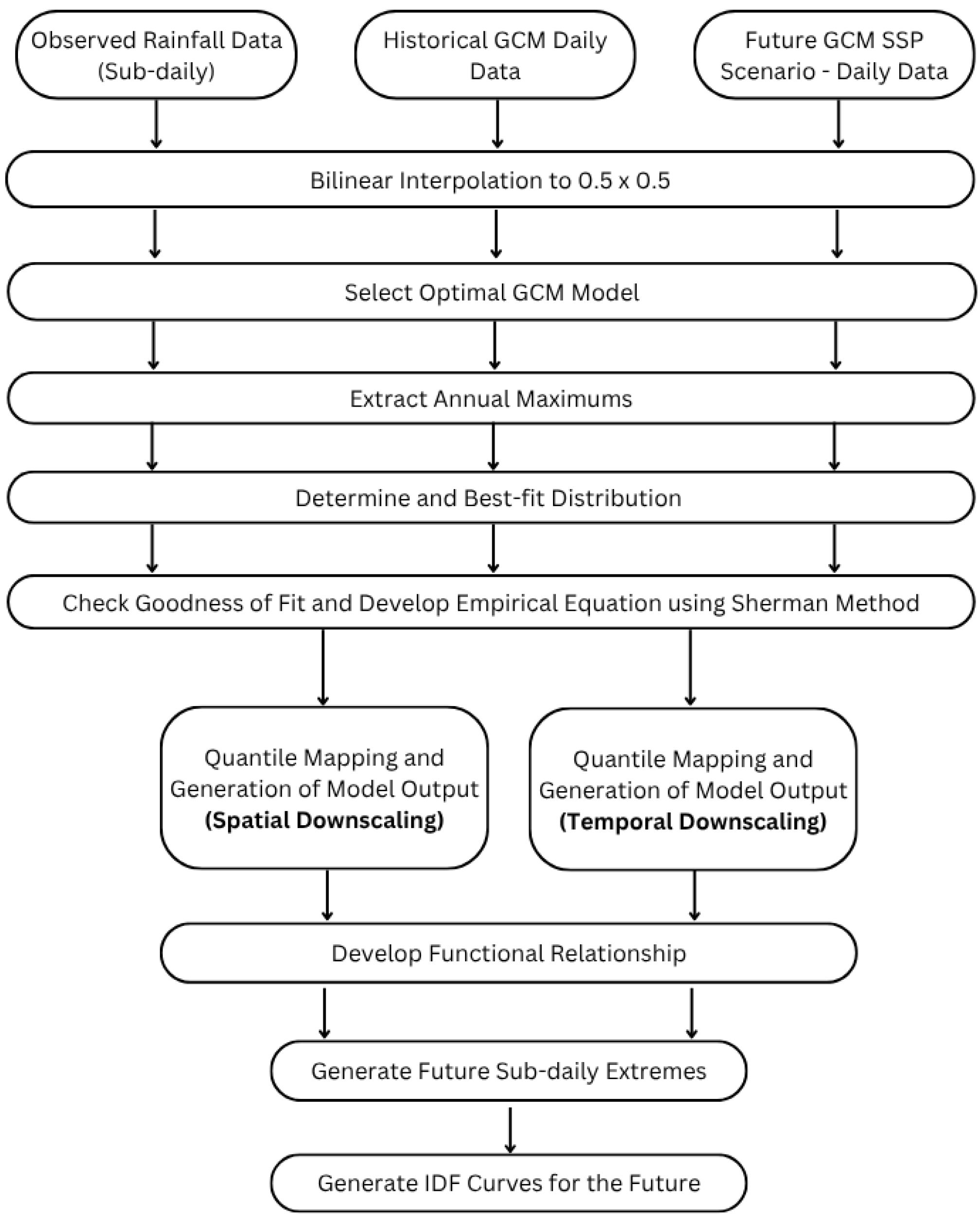
This study aims to develop improved IDF curves under future climate change scenarios for key cities in Punjab, Pakistan. Figure 2 illustrates the methodology used to achieve this goal. The process involved the following steps:
  • Obtain observed and satellite-derived daily rainfall data for the selected cities. Extract GCM numerical simulations for the historical period and future scenarios.
  • Perform bilinear interpolation and extract annual maxima for the obtained rainfall datasets
  • Estimate short duration rainfall (1-h, 2-h, 3-h, 4-h, 6-h, 12-h, and 24-h periods)
  • Identify the optimal GCM model using a ranking method approach and the Taylor diagram
  • Determine the best-fit probability distribution (LP3, GUM, and LN2) for estimating rainfall intensity for the required durations and return periods, using the ranking method and goodness of fit tests.
  • Develop IDF curves for all locations and generate its empirical relations using the Sherman equation.
  • Downscale the satellite-derived dataset using the EQM Method in accordance with the best-fit probability distribution.
  • Generate future projections of updated IDF curves and empirical equations using the downscaled dataset for the defined climate scenarios SSP 2-4.5 and 5-8.5.

3.2. Estimating Short Duration Rainfall

Multiple short durations can be derived from the daily maximum dataset to compute the corresponding rainfall intensities. To obtain the required short-duration rainfall data series, the mostly used formula developed by the Indian Meteorology Department (IMD), also known as the reduction formula, was applied, as shown in Equation (1). Multiple researchers have used this formula for the computation of short-duration data series from daily maximum series [4,7,52,53,54].
P d = P 24 d 24 1 / 3 ,
where Pd represents the depth of rainfall in millimeters for a d-hour duration. The term P24 denotes the maximum daily rainfall depth in millimeters. In this study, short durations of 1 h, 2 h, 3 h, 4 h, 6 h, 12 h, and 24 h were computed using the annual maximum series.

3.3. Selection of Optimal GCM Model

Selecting the most suitable GCM model for downscaling satellite-derived data is crucial [55]. To identify the most suitable GCM for downscaling and future projection, a comprehensive ranking procedure was applied across all candidate models [56]. For each city, the simulated precipitation outputs from the eight selected GCMs were compared with observed datasets for the baseline period (1984–2022). The comparison involved three statistical goodness-of-fit tests (K–S, A–D, and RMSE), where lower test statistic values indicate better model performance. Based on these statistics, each GCM was assigned a rank for every test, with the lowest statistic receiving Rank 1, and so forth. The cumulative rank for each GCM was then computed by summing its individual ranks across the three tests to derive a composite performance score for each city. The GCM with the lowest total rank was considered the most accurate for that location. This procedure was repeated for all five study cities, after which an overall ranking was derived by aggregating the ranks across cities. Additionally, the coefficient of determination (R2) values were computed separately from scatter plots between observed and simulated rainfall data to assess model fidelity. These R2 values were reported alongside the final ranking table, as they were not directly used in the cumulative ranking. The rank-based evaluation was entirely derived from the statistical test performance metrics. These tests assess the model’s goodness of fit, as detailed in Table 3.
The Taylor diagram was used to evaluate the spatial accuracy of the models by comparing satellite-derived and observed patterns [46,57]. It displays three error statistics: the correlation coefficient (R), the centered root mean square error, and the standard deviation (σ). The model with the highest correlation, the lowest error, and a standard deviation closest to that of the observations is considered the most reliable. The Taylor diagram is widely used for assessing climate model performance.

3.4. Selection of Best-Fit Distribution

Before computing intensities and developing IDF empirical equations, the best-fitting probability distribution for the rainfall datasets must be determined [10,58]. This study selected three distributions—Log-Normal Type II (LN2), Log-Pearson Type III (LP3), and Gumbel (GUM)—based on regional research [59,60,61], with previous studies identifying one as the best fit.
The process starts by evaluating the distribution parameters, which assist in computing the required probability distribution functions (PDFs) and cumulative distribution functions (CDFs) for the corresponding distribution. The required distribution parameters include the mean, standard deviation, and coefficient of skewness, calculated using the Equations (2), (3a), and (3b):
S a m p l e   m e a n = X a v g = X i n ,
S t a n d a r d   d e v i a t i o n = σ = 1 n 1 X i X a v g 2 ,
and
C o e f f i c i e n t   o f   s k e w n e s s = γ = n . X i X a v g 3 ( n 1 ) ( n 2 ) S 3 .
Here, n denotes the total number of recorded data points, i refers to the observation index, and Xi represents the ith value in the ordered dataset.
This study takes into account the following frequency/probability distributions:
(1) Log-Normal Distribution: LN2 is commonly utilized in the annual precipitation and surface runoff studies. Both mean and variance are the two parameters that are essential elements of this distribution. Equations (4) and (5) below characterize the PDF and CDF, respectively. In this case, the random variable “x” is defined over a range greater than zero.
f x = 1 x σ Y 2 π exp 1 2 σ Y 2 l n ( x ) μ Y 2
and
F x = 1 σ Y 2 π 0 x 1 x exp 1 2 σ Y 2 l n ( x ) μ Y 2 d x .
(2) Log-Pearson Distribution: LP3 is a frequency distribution similar to the gamma family. It depicts the log-transformed form of the Pearson Type-III distribution variables. Equations (6) and (7) characterize the PDF and CDF, respectively.
f x = 1 | α | x Γ ( β ) l n ( x ) ζ α β 1 exp l n ( x ) ζ α
and
x = 1 | α | Γ ( β ) 0 x 1 x l n ( x ) ζ α β 1 exp l n ( x ) ζ α d x .
With the help of the methods of the moments (MOM) estimators, the parameters—shape β, scale α, and position ζ—are calculated using Equations (8), (9), and (10), respectively as shown below.
β = 4 γ 2 ,
α = σ γ 2 ,
and
ζ = μ 2 σ γ .
(3) Gumbel Distribution: The GUM distribution, classified as Type-I extreme value distribution, is commonly used to estimate the maximum values within a dataset, such as peak discharge. It is widely recognized as one of the most suitable distributions for flood frequency analysis and related hydrological assessments. The corresponding PDF and CDF are presented in Equations (11) and (12) below.
Moreover, the scale parameter α and location parameter β of the distribution are expressed in Equations (13) and (14) below. For the GUM distribution, these parameters are derived through the MOM estimation technique.
f x = 1 α exp x β α exp x β α ,
F x = exp exp x β α ,
α = 0.7797 σ ,
and
β = μ 0.5772 α .
After determining the PDFs and CDFs, goodness-of-fit tests validated the selection process. These included empirical distribution function (EDF) tests, which compare the actual and theoretical datasets [62]. The K–S, A–D, and RMSE tests were applied to identify the optimal probability distribution representing the study area [63,64]. The most suitable probability distribution for each city and rainfall duration was identified separately through a combination of goodness-of-fit evaluations. The distribution with the highest overall ranking across these tests was selected as the best fit for that specific city and rainfall duration. This city-specific approach ensured that the probabilistic representation of rainfall extremes reflects local climatic variability, rather than being averaged across regions. The test statistics, detailed in Table 3, assess the suitability of a distribution for the dataset.
Finally, after the goodness-of-fit tests, the ranking method was applied to determine the best-fitting probability distribution for the rainfall dataset of Punjab cities. The distributions were ranked based on the lowest test statistics, with the distribution showing the best fit being selected.

3.5. Generating IDF Curves and Sherman Equation

IDF curves require data on rainfall intensity (I), duration (D), and return period (F). The rainfall depth data, based on short-duration series calculated using the IMD formula, were used for this. IDF curves for various durations and return periods were developed for each major city in Punjab. Rainfall intensity (I) was first calculated using the rainfall depth (Pd) in millimeters and duration (d) in minutes, as shown in Equation (15):
I = 60 P d d .
After computing the intensity values, the recurrence interval (T) was computed. This was calculated for the available rainfall dataset using the California method, which has been recommended by many researchers for its precise results [33,55,58]. The formula for calculating return period value using the California method is shown in Equation (16):
T = N m ,
where (N) is the number of years for which rainfall data are available, (m) is the rank of the events, and (T) is the return period value calculated in years.
To produce the IDF curves, return periods of 2, 5, 10, 25, 50, and 100 years were specified for this study. Corresponding to these return periods and the earlier defined rainfall durations, rainfall intensities were extracted from the dataset, and the IDF curves for the observed dataset were plotted. After developing the IDF curves for all major cities under consideration using the best-fitting probability distributions, the next step was to formulate the empirical relation/equation for the selected distribution for all cities in the study region. Equations (17) and (18) are known as the Sherman equation, which is considerably accurate and simple to use for the computation of rainfall intensity using a few parameters.
i = a t m = k T x t m
and
a = k T x ,
where i is rainfall intensity (mm/hr), t is the storm duration (minutes), T is the return period (years), and k, x, and a are constants (rainfall intensity parameters, regression parameters, or Sherman coefficients). The coefficient (a), depending on T, is shown in Equation (18). To develop the empirical relation for Punjab’s cities using the Sherman equation, the coefficient values are determined. Equation (17) is linearized (Equation (19)) by applying a logarithmic function (log10 for i and t). A straight-line graph is plotted with log intensity on the y-axis and log duration on the x-axis. The slope gives parameter (m), and the y-intercept gives (loga). Different lines are plotted for return periods (2, 5, 10, 25, and 50 years), varying (loga) while keeping (m) constant. Equation (19) is further linearized (Equation (20)) to account for the frequency factor (a).
log I = log a m log t
and
log a = log k + x log T .
Similarly, a straight-line graph for Equation (20) is plotted, with loga on the y-axis and logT on the x-axis. The loga values are obtained from the graph of Equation (19), and the corresponding logT values are used to generate this graph. The slope of this straight line represents the value of parameter x, and the y-intercept gives the value of logk. Following the defined procedure, the unknown parameters (k, a, and x) can be computed, and the empirical equations for a city can be developed. The procedure is repeated for each major city in the Punjab province, so that a unique and valid empirical equation is developed for each city.

3.6. Downscaling

CMIP6 GCM-simulated data, which provide coarse-resolution projections of future climate, require statistical downscaling to generate localized rainfall estimates suitable for IDF curve development. Such downscaling is particularly important in regions with sparse or unevenly distributed ground stations, where raw GCM outputs may misrepresent local rainfall extremes [65]. To improve the reliability of these projections, GCM-simulated data were corrected using observed station data. Various statistical downscaling methods have been applied globally to enhance the accuracy of climate projections, but many are limited by computational demand, methodological complexity, or higher associated uncertainty [66,67,68,69]. In this study, the EQM method [15] was adopted, as it effectively corrects distributional biases and enables consistent statistical downscaling across multiple emission scenarios [56,69].

3.7. EQM Method Algorithm

One of the essential parts of this study is the downscaling of GCM-simulated precipitation data to ensure an accurate downscaled dataset for the development of future IDF projections. For this purpose, the EQM method was adopted, which is presented stepwise as follows:
  • Select the appropriate GCM model for the study area and obtain the daily maximum rainfall using the historical GCM-simulated daily dataset.
    X m a x G C M = X 1 , m a x G C M X 2 , m a x G C M X 3 , m a x G C M X N , m a x G C M ,
    where the values in the matrix, represented by X i , m a x G C M , are the maximum daily rainfall values from historical GCM-simulated dataset for the ith year, and N is the number of years for which the dataset is available. It is important to note that for the formulation to work effectively, the same time span (number of years) should be used from the observed rainfall dataset.
2.
Using the station/observed rainfall dataset for a location, acquire the sub-daily (1 h, 2 h, 3 h, 4 h, 6 h, 12 h, and 24 h) maximum rainfall values.
X m a x S T N = X 1 , m a x S T N , 1 h r X 1 , m a x S T N , 2 h r X 1 , m a x S T N , 24 h r X 2 , m a x S T N , 1 h r X 2 , m a x S T N , 2 h r X 2 , m a x S T N , 24 h r X 3 , m a x S T N , 1 h r X N , m a x S T N , 1 h r X 3 , m a x S T N , 2 h r X N , m a x S T N , 2 h r X 3 , m a x S T N , 24 h r X N , m a x S T N , 24 h r ,
where the values in the matrix, represented by X i , m a x S T N , j , are the maximum sub-daily rainfall values for a particular location/city (STN) from station/observed rainfall dataset for the jth rainfall duration in the ith year, and N is the number of years for which the dataset is available.
3.
Acquire the daily maximum rainfall using the future GCM-simulated dataset for the defined climate scenarios (i.e., SSP 2-4.5 and 5-8.5).
X m a x G C M , F u t = X 1 , m a x G C M , S S P 2 - 4.5 X 1 , m a x G C M , S S P 5 - 8.5 X 2 , m a x G C M , S S P 2 - 4.5 X 2 , m a x G C M , S S P 5 - 8.5 X 3 , m a x G C M , S S P 2 - 4.5 X N f , m a x G C M , S S P 2 - 4.5 X 3 , m a x G C M , S S P 5 - 8.5 X N f , m a x G C M , S S P 5 - 8.5 ,
where the values in the matrix, represented by X m a x G C M , F u t , are the maximum daily rainfall values from the future GCM-simulated precipitation dataset for the defined climate scenarios, and N f is the number of years considered in the future dataset.
4.
Determine the best-fitting probability distribution representing the daily maximum values obtained from the GCM-simulated (historical and future) dataset and the observed rainfall datasets.
P D F G C M = f θ G C M X m a x G C M ,
P D F j S T N = f θ S T N , j X m a x S T N , j ,
and
P D F G C M , F u t = f θ G C M X m a x G C M , F u t ,
where PDF represents the probability distribution function, and θ is the critical parameter of the best-fitting distribution.
5.
Extract the GCM-simulated sub-daily dataset, Y m a x , j S T N , represents a statistical linkage between the sub-daily dataset and the cumulative probability distribution of the GCM simulation using the quantile mapping methodology. This is also known as spatial downscaling of the historical GCM-simulated dataset to the sub-daily observed rainfall dataset.
Y m a x , j S T N = C D F i n v C D F X m a x G C M / θ G C M / θ S T N , j ,
where CDF represents the cumulative probability distribution function, and invCDF is the inverse of corresponding CDF. Y m a x , j S T N is the sub-daily maximum dataset statistically downscaled for the corresponding jth duration.
6.
With a similar approach, model the variation between the scenario-based future GCM dataset and the historical GCM-simulated dataset using the quantile mapping methodology, which helps extract the downscaled scenario-based future GCM projections, Y m a x G C M , F u t for the dataset. This is known as temporal downscaling of future GCM projections to the baseline historical GCM rainfall dataset:
Y m a x G C M , F u t = C D F i n v C D F X m a x G C M / θ G C M / θ G C M , F u t ,
where Y m a x G C M , F u t is the temporally downscaled dataset for the future GCM projections and the historical GCM simulated dataset for the corresponding period.
7.
Form a suitable function/expression to develop a mathematical relationship between Y m a x , j S T N and X i , m a x G C M . Few studies [10,70] suggest a linear relationship between the two quantities, providing a reasonably accurate relationship. However, this is not valid for all distribution functions. Previous studies have used the Gumbel CDF for this relationship. In this study, the LP3 distribution was identified as the best fit, so its CDF (Equation (29)) is used to develop the first-order linear equation for the two CDFs for the region.
Y m a x , j S T N = f X m a x G C M ,
Y m a x , j S T N = a 1 X m a x G C M + b 1 ,
and
F x = γ k , k e ln x μ β Γ k ,
where γ(k) is the lower partial gamma function, Γ(k) is the complete gamma function, k is the shape parameter, and μ and β are the location and scale parameters.
8.
Following the same approach, determine the function that links Y m a x G C M , F u t and X i , m a x G C M
Y m a x G C M , F u t = f X m a x G C M
and
Y m a x G C M , F u t = a 2 X m a x G C M + b 2 .
9.
To develop future projections of the dataset, combine Equations (17) and (19) along with the replacement of X i , m a x G C M with Y m a x G C M , F u t in Equation (17).
X m a x , j S T N , f u t u r e = a 1 X m a x G C M , f u t u r e b 2 a 2 + b 1 .
10.
Finally, produce IDF curves for the downscaled future projection dataset and compare it with the observed/station-based IDF curves to determine variations in intensities.

4. Results and Discussion

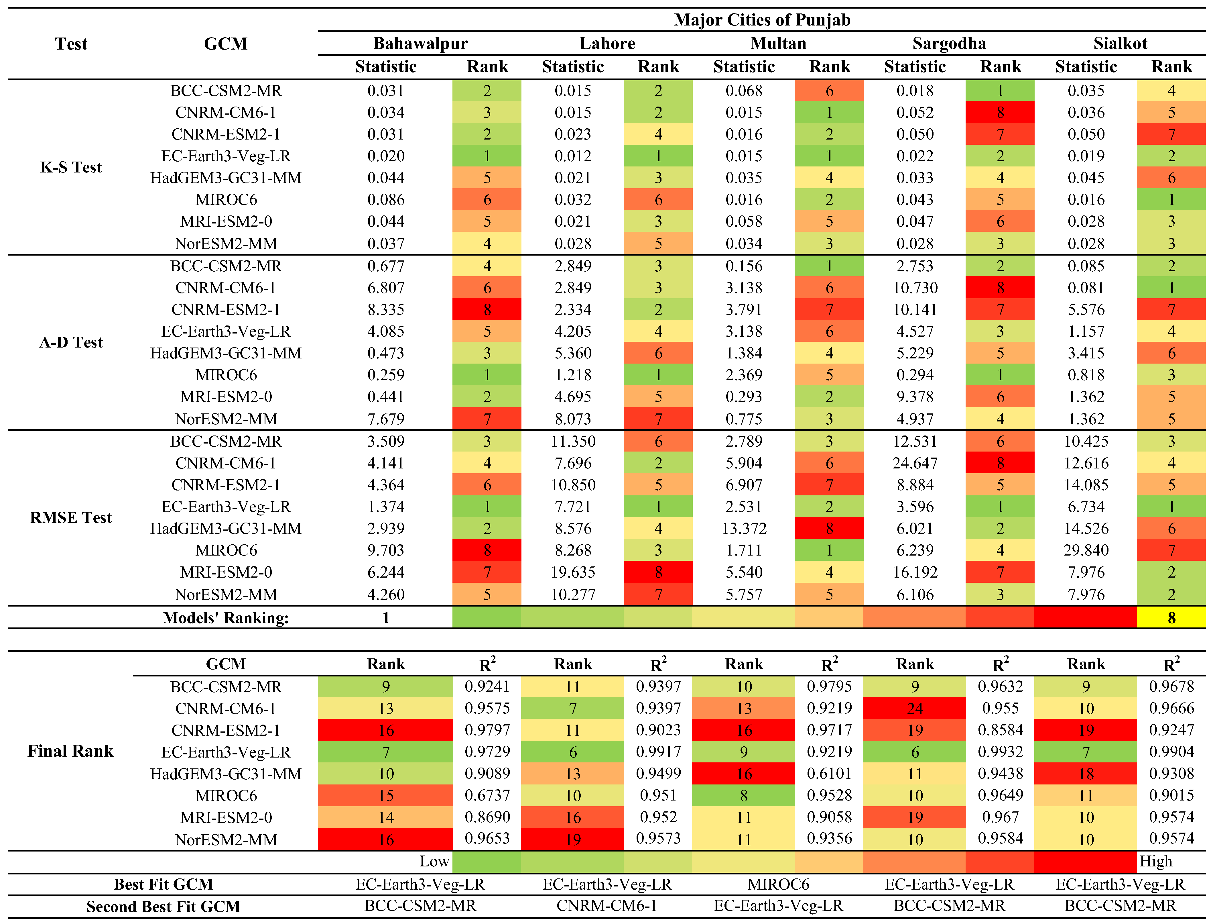
The first step involved selecting the most suitable GCM by evaluating how well various models simulated historical rainfall over the study area. GCM simulation outputs were compared with observed data, and the results, shown in Figure 3 as a heat map, rank the models for Punjab’s major cities based on goodness-of-fit tests. The figure outlines the ranking criteria, emphasizing the need for region-specific assessments due to the spatial variability in GCM performance.
Figure 3 shows a heat map ranking GCMs based on their ability to replicate rainfall patterns in Punjab’s major cities; lighter shades and lower ranks indicate better performance. The EC-Earth3-Veg-LR model was selected for its consistent top ranking. Choosing region-specific GCMs reduces uncertainty in projections [71]. The comparative assessment of GCMs (Figure 3) shows that EC-Earth3-Veg-LR consistently performed best across all five cities, yielding the highest correlation coefficients (R2 = 0.973–0.992) and the lowest RMSE values (1.37–7.72 mm). BCC-CSM2-MR ranked second, with comparable R2 values (0.924–0.968) but slightly higher RMSE. In contrast, models such as MIROC6 and CNRM-ESM2-1 exhibited higher errors (RMSE > 8 mm) and weaker correlations (R2 < 0.90). Overall, EC-Earth3-Veg-LR reduced RMSE by about 65–80% compared with the least accurate models, confirming its superior ability to reproduce observed rainfall characteristics across Punjab. Accordingly, EC-Earth3-Veg-LR and BCC-CSM2-MR were selected for EQM bias correction and subsequent IDF development. Figure 4’s Taylor diagram further summarizes model performance, ensuring the most reliable GCM is used for accurate downscaling and future projections.
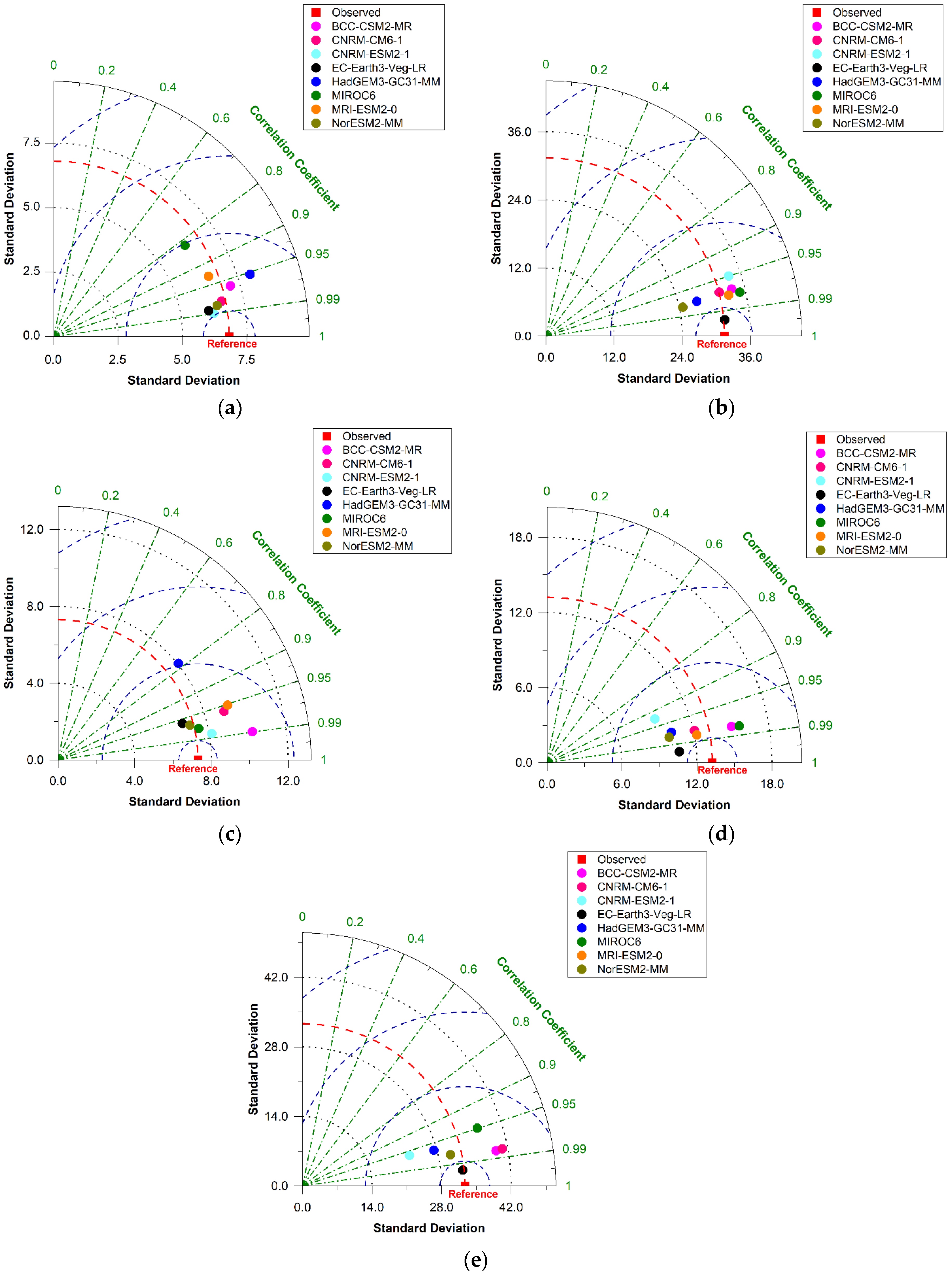
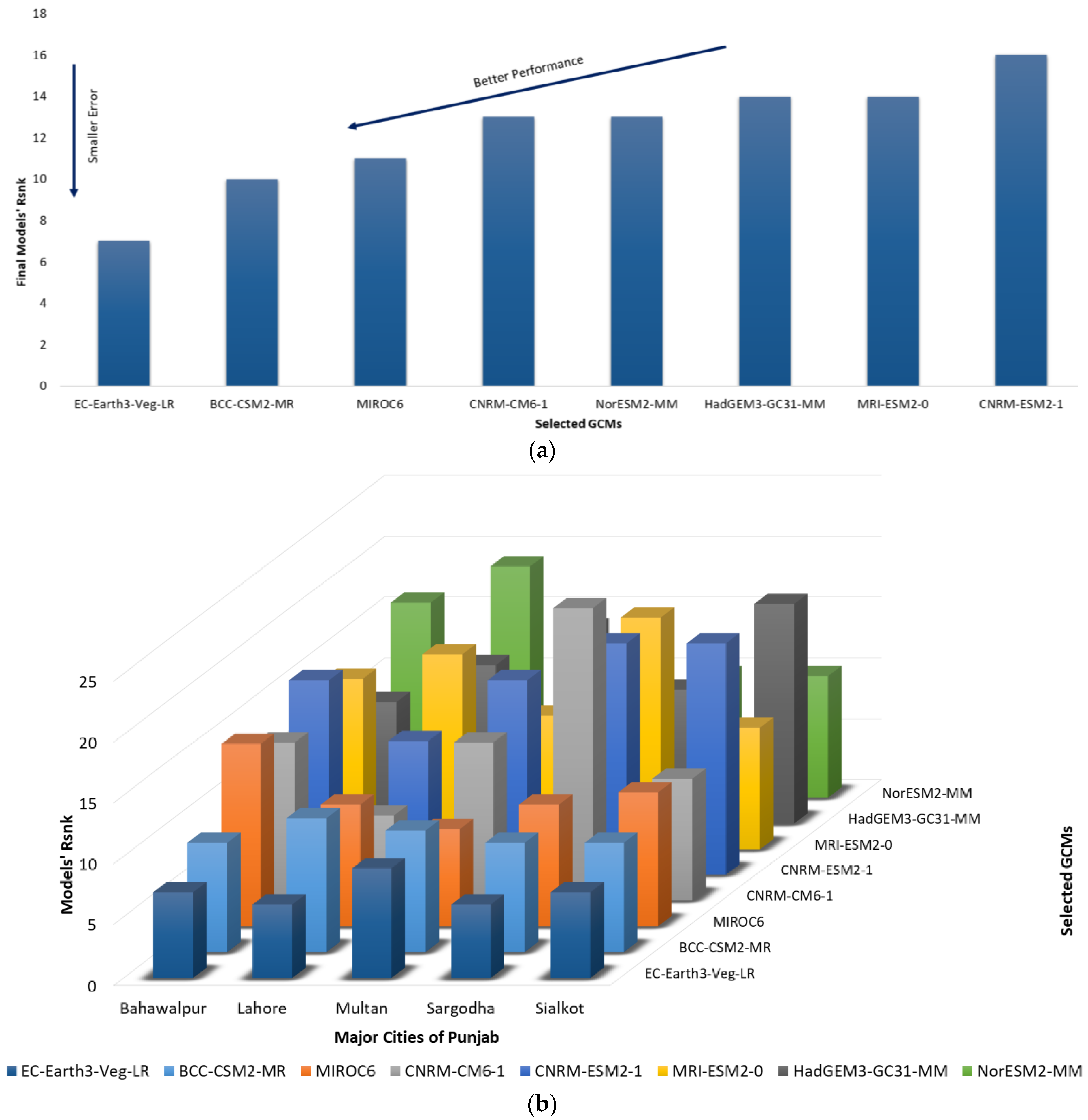
Figure 4 shows the statistical performance of climate models via Taylor diagrams for Bahawalpur, Lahore, Multan, Sargodha, and Sialkot. The results confirm that EC-Earth3-Veg-LR consistently outperforms others, with the highest correlation, lowest RMSE, and standard deviation closest to the observed values. This model was selected for further analysis. A visual summary of GCM performance and rankings across Punjab’s major cities is shown in Figure 5.
The comprehensive GCM ranking presented in Figure 5 highlights the consistent superiority of EC-Earth3-Veg-LR, which attained the lowest overall rank across all stations, indicating the smallest cumulative error and the best rainfall simulation capability. BCC-CSM2-MR followed closely as the second-best model, while MIROC6 and CNRM-ESM2-1 ranked lowest due to higher deviations from observed data. The inter-city ranking confirms that EC-Earth3-Veg-LR achieved top-three performances in all five cities, whereas models with weaker skill exhibited greater spatial inconsistency. Quantitatively, EC-Earth3-Veg-LR outperformed the ensemble average by approximately 60–70% in RMSE reduction and 5–20% in correlation (R2), reaffirming its suitability for EQM bias correction and subsequent IDF curve development.
The second step was to characterize the annual rainfall datasets by identifying the best-fitting probability distribution for the major cities of the province under consideration. The ranking method was adopted for this purpose, and the results are given in Table 4.
Table 4 summarizes the goodness-of-fit test results for ground/station, historical, and future GCM-simulate precipitation data for the major cities in Punjab. Based on the K–S, A–D, and RMSE tests, the LP3 distribution was found as the most suitable for modelling annual maximum rainfall in both historical and projected datasets [72,73]. For observed data, LP3 achieved the lowest K–S (0.010–0.030) and A–D (≈0.03–0.08) statistics together with small RMSE values (0.89–6.20 mm). In the historical GCM-simulated series, LP3 again produced the best overall rank, with RMSE mostly between 1.6 and 3.8 mm, while alternative distributions such as LN2 and GUM yielded higher residuals. Under future projections (SSP2-4.5 and SSP5-8.5), LP3 maintained its superiority, keeping RMSE below ≈9 mm even in cases where other models exceeded 12–14 mm. Quantitatively, LP3 reduced RMSE by roughly 40–60% compared with the second-ranked distribution, demonstrating its robustness for both present and projected rainfall extremes in Punjab. Rainfall intensities for specified durations and return periods were estimated using the best-fitting distribution identified from the goodness-of-fit tests. As LP3 was optimal for the major cities, intensity values were derived from the LP3 dataset. Table 5 summarizes the computed intensities for the defined durations and return periods.
The table shows rainfall intensities for five major cities of Punjab across six return periods and seven durations, based on observed and GCM-simulated data for historical and future scenarios. The results indicate a substantial increase in projected intensities, with 100-year events rising by 40–50% across cities. Intensities also increase notably for shorter durations and higher return periods, emphasizing the need to revise IDF curves to reflect future climate-driven extremes and to guide infrastructure planning.
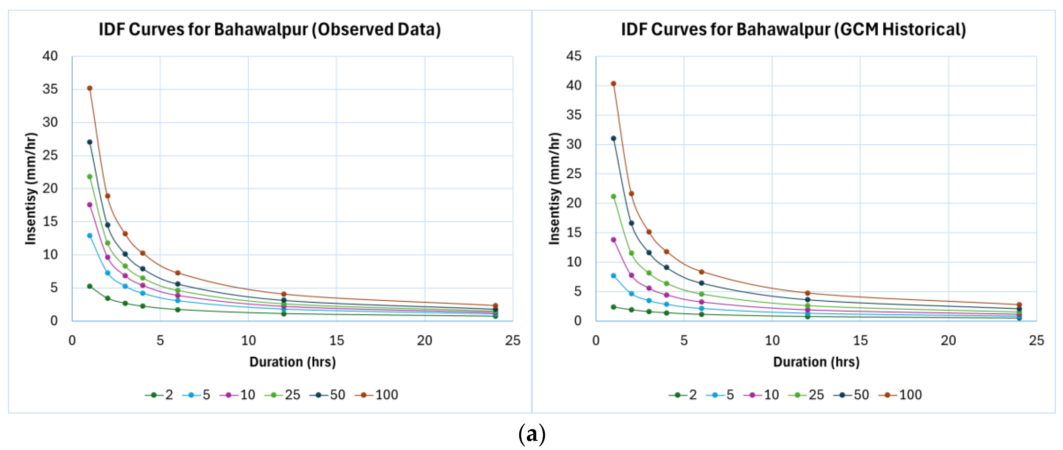
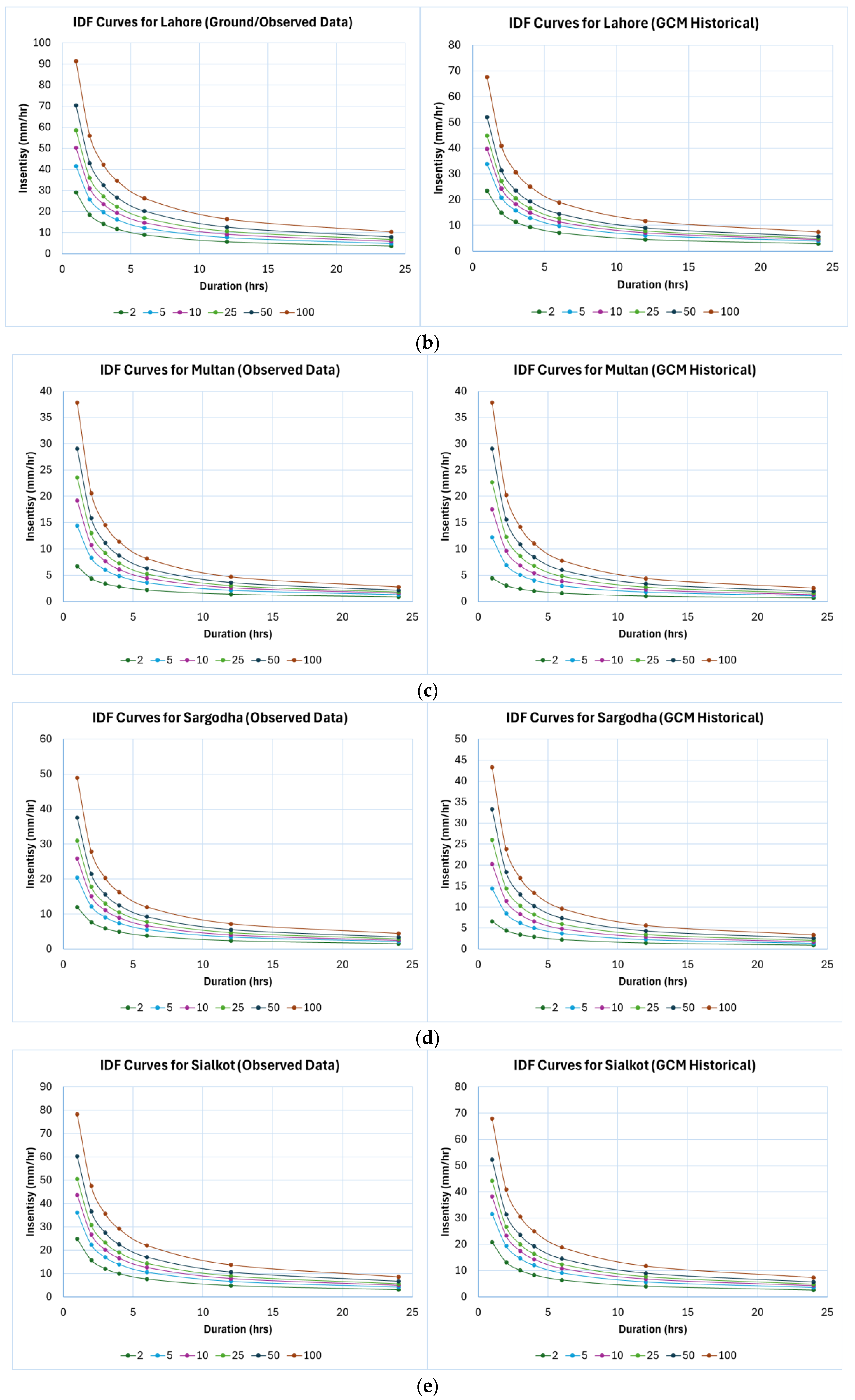
Using the information provided in Table 5, IDF curves for all major cities were prepared using only the ground/observed and GCM-simulated historical datasets, as shown in Figure 6. IDF curves developed using the GCM-simulated future datasets will be presented subsequently, once the corresponding datasets are downscaled, as mentioned earlier.
The pre-downscaling comparison of observed and historical GCM-based IDF curves (Figure 6) indicates that the GCM simulations generally underestimate rainfall intensities, particularly for higher return periods and shorter durations. Across all five cities, the mean underestimation of 100-year intensities is approximately 15–30%, with the largest discrepancies in Lahore and Sialkot, where 1-h observed intensities exceed GCM estimates by up to 25–35%. The differences gradually diminish for longer durations (>12 h), reflecting the GCMs’ coarser temporal resolution and smoothing effect on extreme short-duration rainfall. Despite these deviations, the similarity in curve shapes and the consistent decline of intensity with duration confirm that the GCMs capture the general rainfall scaling behavior, validating their suitability for bias correction using the EQM method.
After developing IDF curves using the best-fitting probability distribution, empirical equations were formulated for each city using the Sherman equation. The required parameters were estimated via a logarithmic approach, as detailed in the methodology. Graphs of Equations (19) and (20) provided the necessary coefficients, which were then applied in Equation (17) to derive the final formulas. Table 6 summarizes the resulting rainfall intensity equations across all data sources, return periods, and durations. These equations, based on both observed and GCM-simulated data for historical and future scenarios, are essential for estimating future intensities and guiding climate-resilient infrastructure design [7].
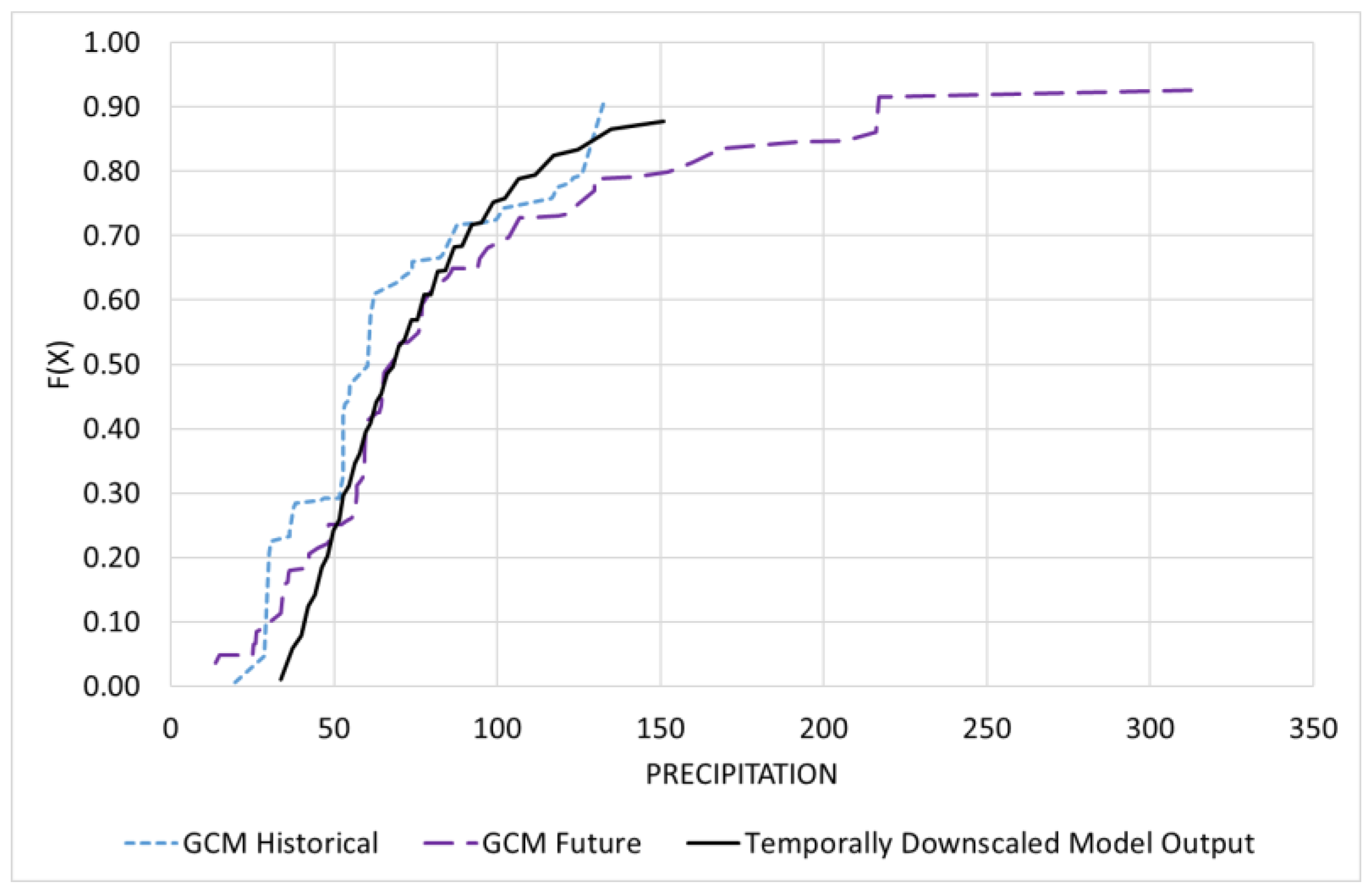
The next crucial step involved downscaling GCM-simulated precipitation datasets for the SSP2-4.5 and SSP5-8.5 scenarios using the EQM method, as detailed earlier. This approach, validated by Srivastav et al. (2014), showed strong agreement between historical and adjusted IDF rainfall intensities [10]. Figure 7 and Figure 8 present the results of spatial and temporal downscaling as an empirical CDF. Spatial downscaling (Figure 7) effectively mirrored the trend of the historical GCM-simulated dataset, while temporal downscaling (Figure 8) established a statistical relationship between historical and future GCM-simulated datasets, thereby improving rainfall IDF projections. Temporal downscaling of future GCM data was performed using the bias-corrected historical GCM distribution derived during spatial downscaling, following the EQM framework proposed by Srivastav et al. (2014) [10].
While EQM bias correction and LP3 frequency modelling have each been used previously in rainfall studies, their explicit coupling for regional IDF projection is uncommon. In this study, the EQM procedure first reduces systematic biases in CMIP6 daily precipitation, improving the fidelity of future projections at the station scale. The LP3 distribution subsequently provides a robust probabilistic framework to translate these bias-corrected projections into IDF relationships. The diagnostic identification of LP3 as the best-fitting distribution for most stations therefore directly reinforces the suitability of this combined approach: EQM improves the input data quality for frequency analysis, and LP3 reliably describes the statistical behavior of extremes in the corrected series. Therefore, this is the first study to integrate EQM downscaling with LP3-based IDF development for major districts in Punjab using CMIP6 projections, providing a practical pipeline from bias-corrected climate projections to usable, station-specific IDF equations for design and planning.
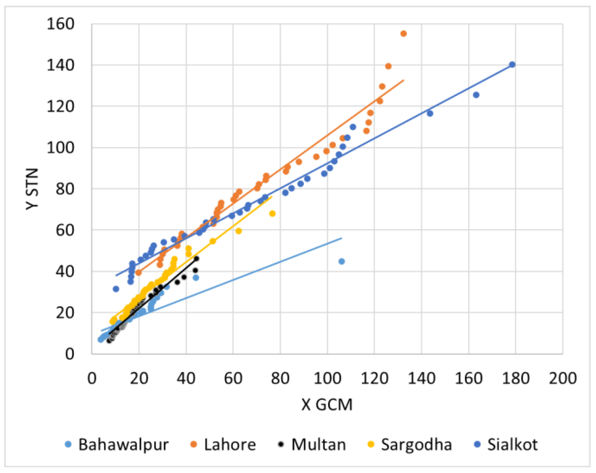
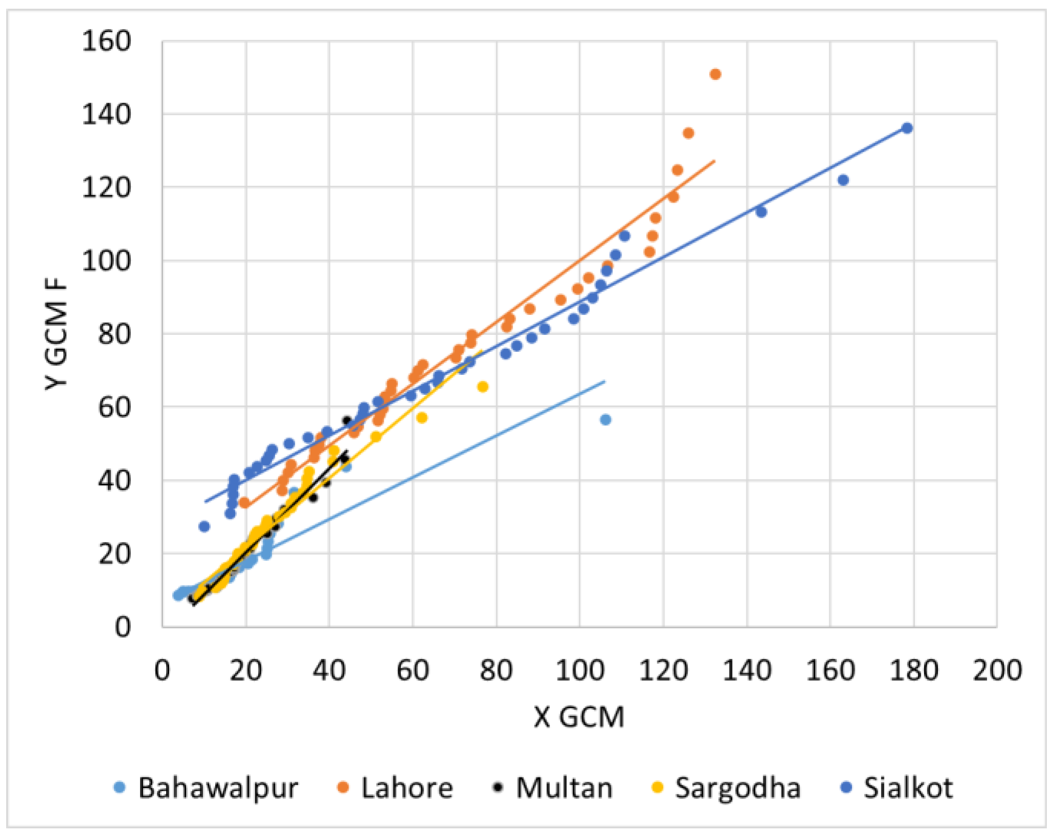
The spatial and temporal downscaling equations produced a first-order linear relationship, derived from the LP3 mapping functions, which are shown in Figure 9, Figure 10 and Figure 11. The figures clearly demonstrate that, for all the major cities considered in this study, a linear relationship exists between the concerned variables for downscaling [70]. Figure 9 represents the relationship derived from the EQM method for spatial downscaling, whereas Figure 10 and Figure 11 show the relationships for temporal downscaling under SSP 2-4.5 and 5-8.5, respectively.
Following the defined procedure, the downscaled GCM-simulated datasets for both climate scenarios were obtained and validated through visual representation and statistical techniques, as presented earlier. Table 7 below shows an analytical summary of the computed downscaled maximum rainfall intensities intended for the defined duration of 1 h and multiple return periods for major cities in Punjab.
Table 7 presents the percentage changes in rainfall intensities for future climate scenarios, before and after EQM downscaling. Across all cities, downscaling improved the agreement with observed values by reducing GCM bias by approximately 5–25%, depending on duration and return period. The effect was most notable for shorter durations (2–10 h), where raw GCM outputs typically underestimated intensities. Under the SSP2-4.5 scenario, EQM correction reduced underestimation in Bahawalpur and Multan by up to 27–30%, while in Lahore and Sialkot, intensities increased by 6–10%, aligning more closely with observations. In future projections, rainfall intensities are likely to increase by 20–45% under SSP5-8.5 relative to historical conditions, with the largest amplification in urban centers such as Lahore and Sargodha. These results demonstrate that EQM-based downscaling effectively corrects systematic GCM biases and captures the projected intensification of extreme rainfall under warming scenarios.
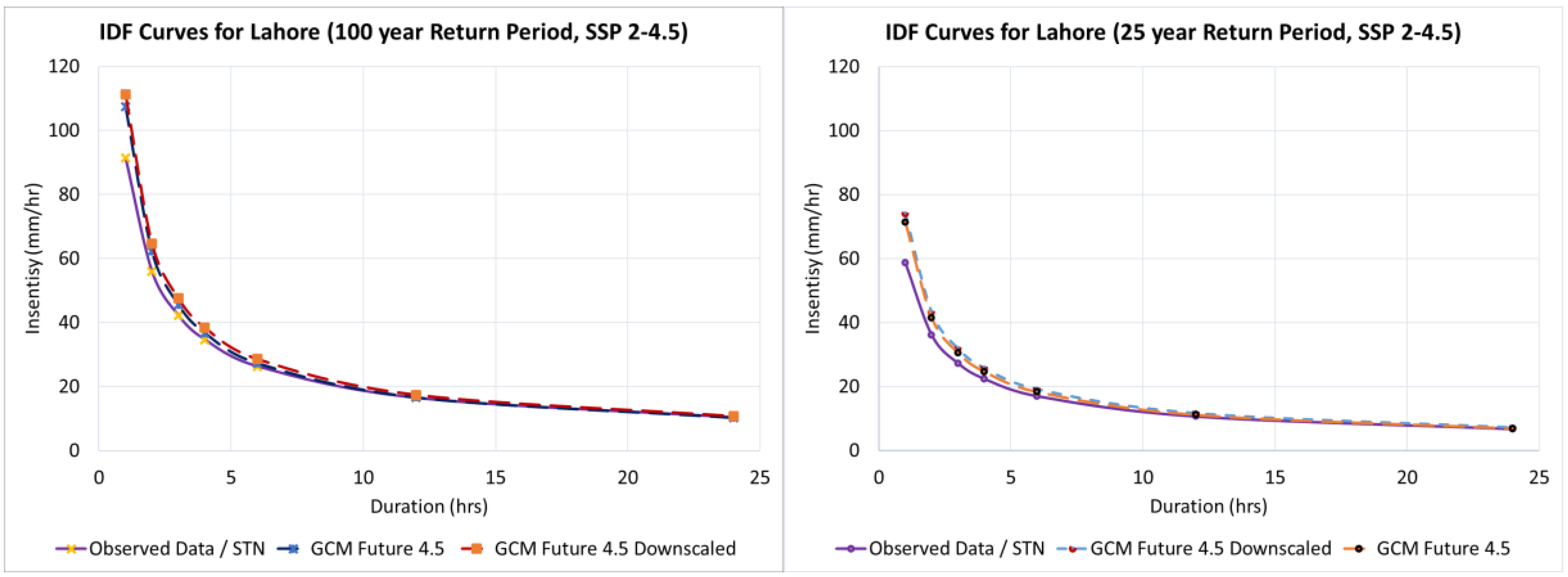
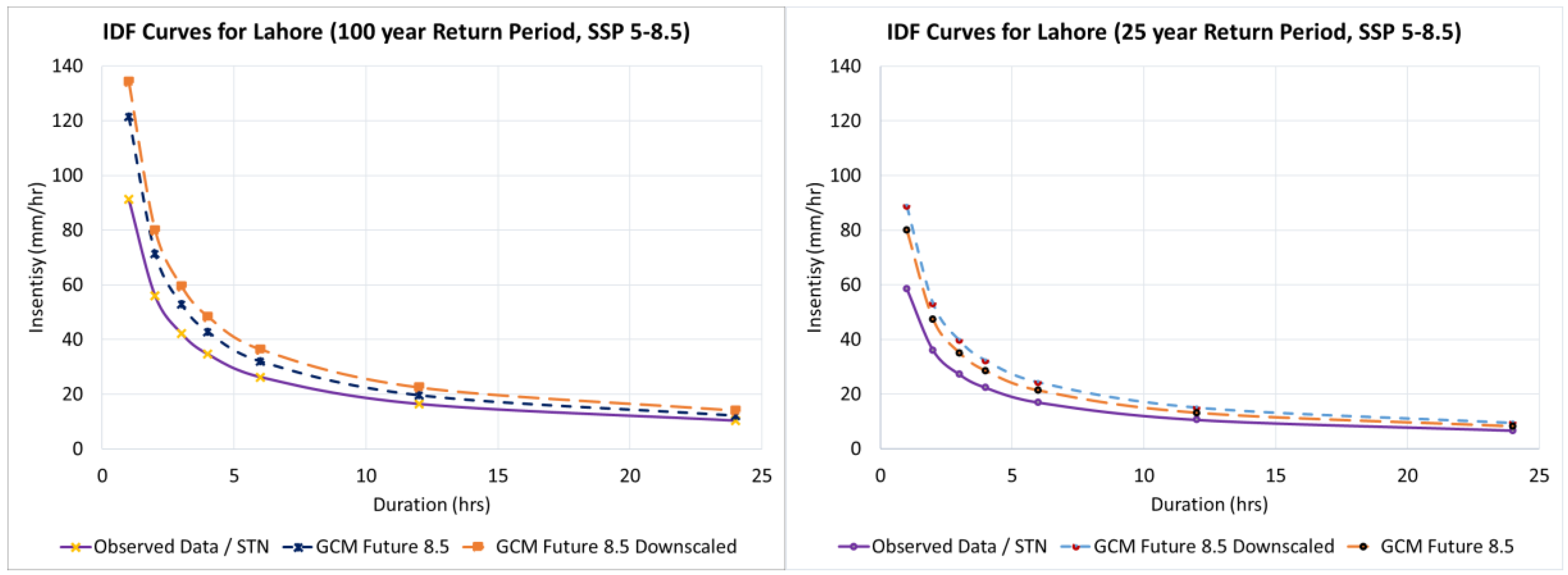
Figure 12 and Figure 13 represent the updated IDF curves for Lahore city, corresponding to SSP 2-4.5 and 5-8.5 scenarios, for 25- and 100-year return periods. The effect of downscaling the future GCM datasets for the climate scenarios considered can be clearly seen from these figures.
The analytical summary in Table 7 presents several noteworthy findings:
  • The updated IDF curves show a consistent increase across intensifying SSP scenarios, with the highest changes under SSP5-8.5 [74].
  • Downscaled GCM datasets project a significant rise in rainfall intensities for major cities in Punjab, improving future projections’ accuracy compared to raw GCM outputs.
  • Rainfall intensities increase more under the SSP5-8.5 scenario than SSP2-4.5 [75], highlighting the impact of greenhouse gas emissions.
  • The downscaling process significantly affected future projections, especially for extreme return periods; for Lahore, the 100-year intensity increased by about 10% under SSP5-8.5.
  • Rainfall intensities increased most in Multan, followed by Bahawalpur, Sargodha, Lahore, and Sialkot, with critical implications for infrastructure design [76]. Historical rainfall intensities show typical trends for Punjab’s major urban centers, with Lahore being the wettest and Bahawalpur the driest [76].
  • SSP5-8.5 shows a higher percentage change than SSP2-4.5 across rainfall durations. Bahawalpur’s 50-year return period intensity increases by 95.72% under SSP2-4.5, and Lahore’s by 26.23%.
  • Under SSP5-8.5, future projections show a larger increase, with Bahawalpur’s 50-year return period intensity rising by 111.39%, and Lahore’s by 51.56%.
  • Downscaled GCM projections are generally lower than raw data but show significant increases compared to historical observations [77].
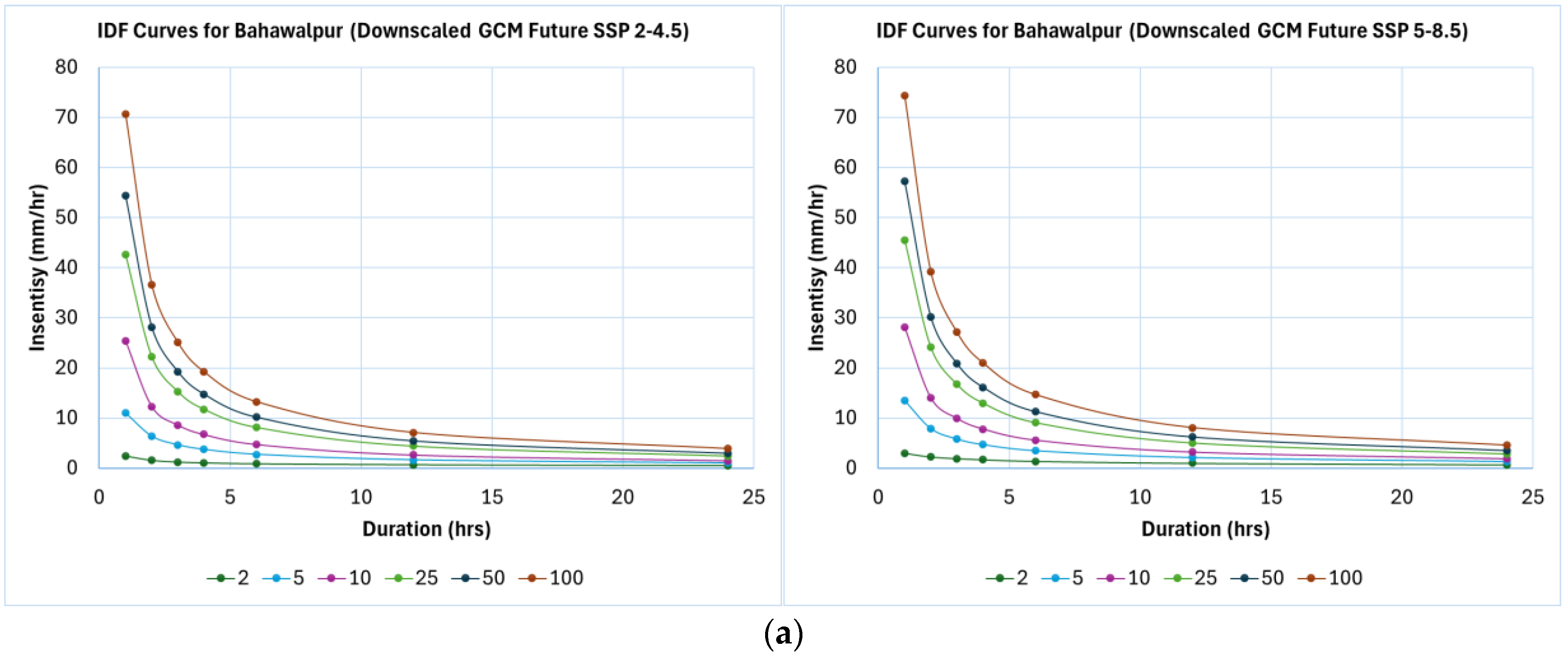
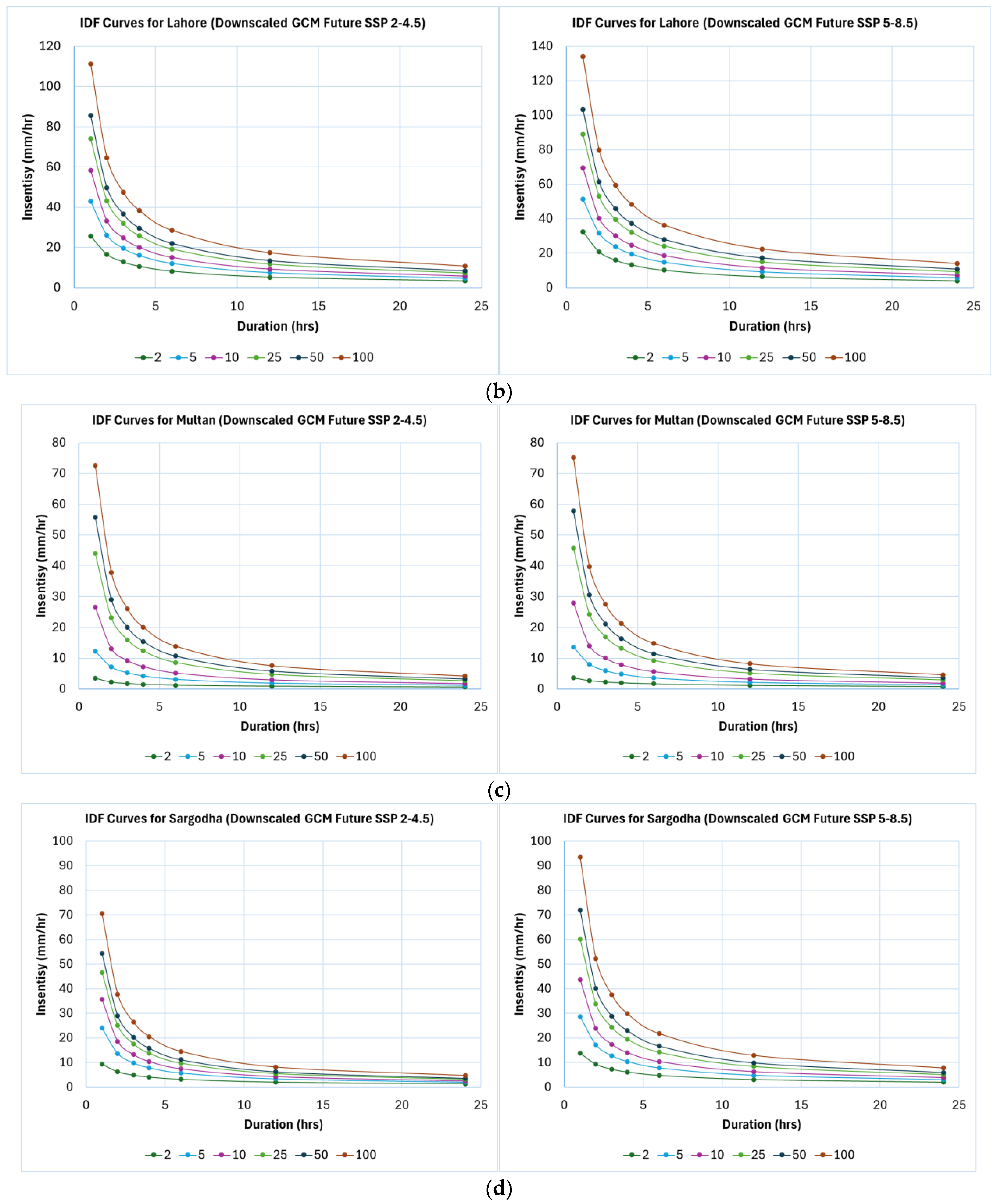
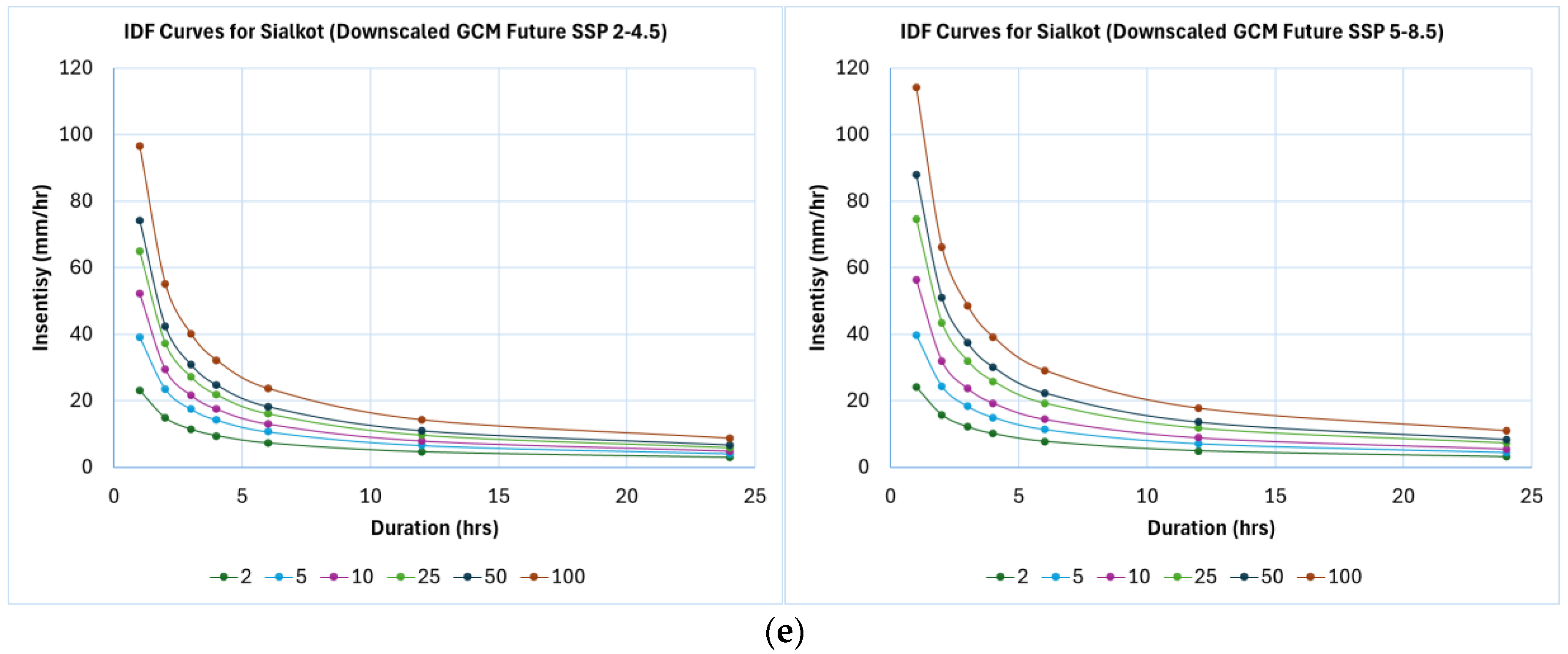
These results suggest that cities in Punjab will face significant challenges due to increased rainfall intensities, requiring adaptation and mitigation strategies to protect water resources, agriculture, and infrastructure [74,76,78]. Downscaled GCM-simulated data are crucial for accurate climate impact studies, as satellite-derived datasets tend to overestimate changes. The findings indicate a significant increase in future rainfall intensities, especially under higher emissions scenarios, with implications for urban planning, infrastructure design, and water resource management [73,76,79]. Figure 14 presents the updated IDF curves, and Table 8 shows the updated rainfall intensity equations for downscaled GCM-simulated datasets, which can aid in designing and managing climate-resilient water infrastructure.
The table presents updated empirical formulas for rainfall IDF curves using downscaled GCM-simulated datasets. The results show significant increases in rainfall intensities, especially under SSP5-8.5. For Lahore, the 100-year rainfall intensity is projected to rise by 25% under SSP2-4.5 and by 30% under the downscaled SSP2-4.5 scenario. Under SSP5-8.5, the increase is 44%, with a 55% rise for the downscaled projections. The downscaling process results in a 3% increase under SSP2-4.5 and an 8.5% increase under SSP5-8.5 [80,81,82].
The updated IDF curves presented in Figure 14 show a clear intensification of rainfall extremes across all five cities under future climate scenarios. Compared with historical conditions, projected 100-year rainfall intensities increase by approximately 20–35% under SSP2-4.5 and 35–55% under SSP5-8.5, with the most pronounced rise observed in Lahore and Sargodha. Short-duration storms (2–6 h) exhibit the strongest relative increase, indicating a potential escalation of flash-flood risk in urban areas. The curves for Bahawalpur and Multan, while showing smaller absolute intensities, still display consistent upward shifts of 10–25%, reflecting broader regional intensification trends. Overall, the downscaled IDF relationships capture both spatial and scenario-driven variations in rainfall extremes, underscoring the growing influence of a warming climate on hydrological design parameters in Punjab.
The downscaling process was crucial, yielding lower projected increases than raw GCM data, though changes are still substantial. These findings emphasize the importance of downscaled climate data for assessing local impacts of climate change. They underline the need for adaptation and mitigation strategies in Punjab’s major cities to address future increases in rainfall intensities. Spatial differences observed in the IDF curves across the five study cities can be attributed to both geographical and climatic factors. Cities located in the northern part of Punjab, such as Sialkot, are influenced by hilly terrain and orographic effects, which enhance precipitation intensity compared to the relatively flat and arid regions of southern Punjab, such as Multan and Bahawalpur. Additionally, variations in atmospheric water vapor availability contribute to these differences, as areas with higher humidity are more prone to short-duration extreme rainfall events. Under a warming climate—particularly under the SSP5-8.5 scenario—enhanced convective activity and the greater atmospheric moisture-holding capacity (approximately 7% per °C, following the Clausius–Clapeyron relation) lead to a disproportionate increase in short-duration rainfall intensities. These processes collectively help explain the differences in IDF curves across the study region and underscore the importance of considering both topographic and climatic drivers when developing future design standards.
Although the results demonstrate clear and consistent trends, certain uncertainties should be acknowledged. Differences among CMIP6 models introduce inter-model variability, especially in simulating convective rainfall and short-duration extremes, which may contribute to the spread in projected intensities. The EQM bias correction, while effective in improving GCM performance, assumes stationarity in the bias structure and may not fully capture non-linear future changes in precipitation behavior. Additionally, the selection of the LP3 distribution and the limited number of high-quality rainfall stations could introduce regional uncertainty and potential overfitting in specific areas. Nevertheless, the use of multiple GCMs, rigorous validation, and the consistent agreement between observed and downscaled GCM-simulated datasets enhance the robustness of the projections and support the reliability of the derived IDF relationships.
This study aligns with previous research on climate change impacts on water resources in the Hindukush–Karakorum–Himalaya region [83] and rainfall erosivity in central India [76]. It contributes to the growing literature on climate change effects in South Asia, particularly Pakistan, showing significant future increases in rainfall intensities, especially under extreme emission scenarios. These findings are consistent with projections of increased runoff and water availability in the Indian subcontinent [80]. However, this study specifically focuses on updating rainfall IDF curves for Punjab’s major cities, offering localized insights for urban planning and water management.

5. Conclusions

This study projects future rainfall IDF curves for major cities in Punjab, Pakistan, using downscaled CMIP6 GCM-simulated data. Results show significant increases in rainfall intensities across all durations and return periods, especially under the higher emissions scenario (SSP5-8.5). The downscaled projections indicate a sharper rise in intensities compared to raw GCM data, emphasizing the value of high-resolution climate data for local impact assessments. The updated IDF equations can aid water resources planners, engineers, and policymakers in managing infrastructure under changing climate conditions. The spatial variability in the updated IDF curves also reflects the influence of topography and atmospheric moisture availability, with northern hilly regions experiencing stronger orographic effects than the drier plains. These insights reinforce the importance of incorporating both climatic and geographic factors when applying IDF projections for design and planning. These findings are crucial for enhancing urban resilience to climate change-induced water challenges, such as frequent and intense flooding.
The projected escalation of rainfall extremes carries profound implications for Punjab’s rapidly urbanizing landscape. Cities such as Lahore and Sialkot, characterized by dense populations and limited drainage capacity, face an elevated risk of severe urban flooding and infrastructure stress. In contrast, cities like Multan and Bahawalpur, though less densely populated, remain highly susceptible to stormwater accumulation due to flat terrain and slower runoff. Sargodha, with moderate population density, represents an intermediate vulnerability profile where both hydrological and infrastructural limitations converge. These contrasting urban dynamics underscore that the consequences of intensifying rainfall will not be uniform but instead will amplify existing disparities in resilience and preparedness across municipalities. Hence, the findings of this study provide an essential scientific foundation for developing city-specific adaptation frameworks, prioritizing climate-resilient infrastructure, and guiding evidence-based policymaking to safeguard the socio-economic stability of Punjab’s urban centers under a changing climate.

Author Contributions

Conceptualization, F.H., S.A. and B.Đ.; data curation, N.A.; formal analysis, F.H., W.S.A., B.Đ. and Y.M.Y.; funding acquisition, Y.M.Y.; investigation, S.A., N.A. and B.Đ.; methodology, F.H.; project administration, W.S.A.; resources, N.A. and Y.M.Y.; software, F.H. and N.A.; supervision, S.A. and N.A.; validation, S.A.; visualization, F.H., W.S.A. and Y.M.Y.; writing—original draft, F.H., N.A. and Y.M.Y.; writing—review and editing, N.A., W.S.A., B.Đ. and Y.M.Y. All authors have read and agreed to the published version of the manuscript.

Funding

This research was funded by the Princess Nourah bint Abdulrahman University Researchers Supporting Project number (PNURSP2025R680), Princess Nourah bint Abdulrahman University, Riyadh, Saudi Arabia.

Institutional Review Board Statement

Not applicable.

Informed Consent Statement

Not applicable.

Data Availability Statement

The original contributions presented in this study are included in the article; further inquiries can be directed to the corresponding author.

Acknowledgments

The authors extend their appreciation to the Princess Nourah bint Abdulrahman University Researchers Supporting Project number (PNURSP2025R680), Princess Nourah bint Abdulrahman University, Riyadh, Saudi Arabia. The authors are also grateful to the National University of Computer and Emerging Sciences (NUCES) for providing the required facilities. We are also thankful to the Pakistan Meteorological Department (PMD) for providing the data for this research.

Conflicts of Interest

The authors declare no conflicts of interest.

References

  1. Shreyas, R.; Punith, D.; Bhagirathi, L.; Krishna, A.; Devagiri, G.M. Exploring Different Probability Distributions for Rainfall Data of Kodagu—An Assisting Approach for Food Security. Int. J. Curr. Microbiol. Appl. Sci. 2020, 9, 2972. [Google Scholar] [CrossRef]
  2. Alasgah, A.A.; Ahmad, I.; Dar, M.A.; Youssef, Y.M.; Zeleňáková, M.; Sisay, M.; Zewdu, G.S.; Heiba, Y. Integrating GIS–Fuzzy Logic Framework and Remotely Sensed Climate Data for Drought Vulnerability Assessment across Africa. Environ. Monit. Assess. 2025, 197, 1110. [Google Scholar] [CrossRef] [PubMed]
  3. Hawkins, E.; Frame, D.J.; Harrington, L.J.; Joshi, M.; King, A.D.; Rojas, M.; Sutton, R. Observed Emergence of the Climate Change Signal: From the Familiar to the Unknown. Geospat. Res. Lett. 2020, 47. [Google Scholar] [CrossRef]
  4. Majeed, A.R.; Nile, B.K.; Al-Baidhani, J.H. Selection of Suitable PDF Model and Build of IDF Curves for Rainfall in Najaf City, Iraq. J. Phys. Conf. Ser. 2021, 1973, 12184. [Google Scholar] [CrossRef]
  5. Dass, B.; Sen, S.; Sharma, A.; Hussain, S.; Rana, N.; Sen, D. Hydrological Process Monitoring for Springshed Management in the Indian Himalayan Region: Field Observatory and Reference Database. Curr. Sci. 2021, 120, 791. [Google Scholar] [CrossRef]
  6. Youssef, Y.M.; AlMetwaly, W.M.; Saber, M.; Abdelshafy, M.; Qaysi, S.; Al-Arifi, N.; Wahba, M. Integrating Geospatial and Hydrodynamic Modelling to Unravel Cultural Heritage Vulnerability to Dam Breaches and Flash Flood in Arid Environments. Int. J. Disaster Risk Reduct. 2025, 126, 105605. [Google Scholar] [CrossRef]
  7. Basumatary, V.; Sil, B.S. Generation of Rainfall Intensity-Duration-Frequency Curves for the Barak River Basin. Meteorol. Hydrol. Water Manag. 2017, 6, 47–57. [Google Scholar] [CrossRef]
  8. Otto, F.E.L.; Zachariah, M.; Saeed, F.; Siddiqi, A.; Shahzad, K.; Mushtaq, H.; Arulalan, T.; AchutaRao, K.; Chaithra, S.T.; Barnes, C.; et al. Climate Change Likely Increased Extreme Monsoon Rainfall, Flooding Highly Vulnerable Communities in Pakistan. Environ. Res. Clim. 2023, 2, 025001. [Google Scholar] [CrossRef]
  9. Yan, X.; Xu, K.; Feng, W.; Chen, J. A Rapid Prediction Model of Urban Flood Inundation in a High-Risk Area Coupling Machine Learning and Numerical Simulation Approaches. Int. J. Disaster Risk Sci. 2021, 12, 903. [Google Scholar] [CrossRef]
  10. Srivastav, R.K.; Schardong, A.; Simonovic, S.P. Equidistance Quantile Matching Method for Updating IDF Curves under Climate Change. Water Resour. Manag. 2014, 28, 2539–2562. [Google Scholar] [CrossRef]
  11. Anand, S.; Kumar, P.; Kumar, M. Development of Rainfall Intensity-Duration-Frequency Relationships and Nomographs for Selected Stations in Maharashtra, India. MAUSAM 2023, 74, 707. [Google Scholar] [CrossRef]
  12. Mahdi, E.S.; Mohamedmeki, M.Z. Analysis of Rainfall Intensity-Duration-Frequency (IDF) Curves of Baghdad City. IOP Conf. Ser. Mater. Sci. Eng. 2020, 888, 12066. [Google Scholar] [CrossRef]
  13. Tabari, H. Climate Change Impact on Flood and Extreme Precipitation Increases with Water Availability. Sci. Rep. 2020, 10, 13768. [Google Scholar] [CrossRef] [PubMed]
  14. Nurfaida, W.; Ramdhani, H.; Shimozono, T.; Triawati, I.; Sulaiman, M. Rainfall Trend and Variability over Opak River Basin, Yogyakarta, Indonesia. J. Civ. Eng. Forum 2021, 7, 109–120. [Google Scholar] [CrossRef]
  15. Li, H.; Sheffield, J.; Wood, E.F. Bias Correction of Monthly Precipitation and Temperature Fields from Intergovernmental Panel on Climate Change AR4 Models Using Equidistant Quantile Matching. J. Geophys. Res. Atmos. 2010, 115, D10101. [Google Scholar] [CrossRef]
  16. Schardong, A.; Simonović, S.P.; Gaur, A.; Sandink, D. Web-Based Tool for the Development of Intensity Duration Frequency Curves under Changing Climate at Gauged and Ungauged Locations. Water 2020, 12, 1243. [Google Scholar] [CrossRef]
  17. Scafetta, N. Impacts and Risks of “Realistic” Global Warming Projections for the 21st Century. Geosci. Front. 2023, 15, 101774. [Google Scholar] [CrossRef]
  18. Zhu, J. Impact of Climate Change on Extreme Rainfall across the United States. J. Hydrol. Eng. 2012, 18, 1301. [Google Scholar] [CrossRef]
  19. Rohat, G.; Flacke, J.; Dao, H.; Maarseveen, M.F.A.M. van Co-Use of Existing Scenario Sets to Extend and Quantify the Shared Socioeconomic Pathways. Clim. Change 2018, 151, 619. [Google Scholar] [CrossRef]
  20. Yang, S.; Cui, X. Review Building Regional Sustainable Development Scenarios with the SSP Framework. Sustainability 2019, 16, 5712. [Google Scholar] [CrossRef]
  21. Ayek, A.A.E.; Loho, M.A.; Alkhuraiji, W.S.; Eid, S.; Abd-Elmaboud, M.E.; Nahas, F.; Youssef, Y.M. Deciphering Air Pollution Dynamics and Drivers in Riverine Megacities Using Remote Sensing Coupled with Geospatial Analytics for Sustainable Development. Atmosphere 2025, 16, 1084. [Google Scholar] [CrossRef]
  22. Sun, Y.; Wendi, D.; Kim, D.E.; Liong, S. Deriving Intensity–Duration–Frequency (IDF) Curves Using Downscaled in Situ Rainfall Assimilated with Remote Sensing Data. Geosci. Lett. 2019, 6, 17. [Google Scholar] [CrossRef]
  23. Marra, F.; Morin, E.; Peleg, N.; Mei, Y.; Anagnostou, E.N. Intensity–Duration–Frequency Curves from Remote Sensing Rainfall Estimates: Comparing Satellite and Weather Radar over the Eastern Mediterranean. Hydrol. Earth Syst. Sci. 2017, 21, 2389. [Google Scholar] [CrossRef]
  24. Xu, L.; Chen, N.; Moradkhani, H.; Zhang, X.; Hu, C. Improving Global Monthly and Daily Precipitation Estimation by Fusing Gauge Observations, Remote Sensing, and Reanalysis Data Sets. Water Resour. Res. 2020, 56, e2019WR02644. [Google Scholar] [CrossRef]
  25. Awatade, S.; Kashiwar, S.R.; Ghosh, S.; Singhandhupe, R.B.; Dongarwar, U.R.; Dhakre, D.S. Satellite Based Estimation and Validation of Rainfall Distribution in Monsoon over Washim (Maharashtra), India. Int. J. Curr. Microbiol. Appl. Sci. 2018, 7, 1694. [Google Scholar] [CrossRef]
  26. Khan, N.; Shahid, S.; Ahmed, K.; Wang, X.; Ali, R.; Ismail, T.; Nawaz, N. Selection of GCMs for the Projection of Spatial Distribution of Heat Waves in Pakistan. Atmos. Res. 2019, 233, 104688. [Google Scholar] [CrossRef]
  27. Iqbal, Z.; Shahid, S.; Ahmed, K.; Ismail, T.; Nawaz, N. Spatial Distribution of the Trends in Precipitation and Precipitation Extremes in the Sub-Himalayan Region of Pakistan. Theor. Appl. Climatol. 2019, 137, 2755. [Google Scholar] [CrossRef]
  28. Ren, H.; Hou, Z.; Wigmosta, M.S.; Liu, Y.; Leung, L.R. Impacts of Spatial Heterogeneity and Temporal Non-Stationarity on Intensity-Duration-Frequency Estimates—A Case Study in a Mountainous California-Nevada Watershed. Water 2019, 11, 1296. [Google Scholar] [CrossRef]
  29. Loho, M.A.; Ayek, A.A.E.; Alkhuraiji, W.S.; Eid, S.; Rebouh, N.Y.; Abd-Elmaboud, M.E.; Youssef, Y.M. Assessing Environmental Sustainability in the Eastern Mediterranean Under Anthropogenic Air Pollution Risks Through Remote Sensing and Google Earth Engine Integration. Atmosphere 2025, 16, 894. [Google Scholar] [CrossRef]
  30. Mahmud, M.R.; Hashim, M.; Matsuyama, H.; Numata, S.; Hosaka, T. Spatial Downscaling of Satellite Precipitation Data in Humid Tropics Using a Site-Specific Seasonal Coefficient. Water 2018, 10, 409. [Google Scholar] [CrossRef]
  31. Hochman, A.; Kunin, P.; Alpert, P.; Harpaz, T.; Saaroni, H.; Rostkier-Edelstein, D. Weather Regimes and Analogues Downscaling of Seasonal Precipitation for the 21st Century: A Case Study over Israel. Int. J. Climatol. 2019, 40, 2062. [Google Scholar] [CrossRef]
  32. Ekström, M.; Grose, M.R.; Whetton, P.H. Advanced Review An Appraisal of Downscaling Methods Used in Climate Change Research. Wiley Interdiscip. Rev. Clim. Change 2015, 6, 301–319. [Google Scholar] [CrossRef]
  33. Fathy, I.; Negm, A.M.; El-Fiky, M.; Nassar, M.; Al-Sayed, E. Intensity Duration Frequency Curves for Sinai Peninsula, Egypt. Int. J. Res. Eng. Technol. 2014, 2, 105–112. [Google Scholar]
  34. Gebreigziabher, E.T. Analysis Rainfall Intensity-Duration-Frequencyrelationships Under Climate Change for Mekele City, Ethiopia. Int. J. Tech. Res. Sci. 2020, 5, 1. [Google Scholar] [CrossRef]
  35. Pierce, D.W.; Cayan, D.R.; Maurer, E.P.; Abatzoglou, J.T.; Hegewisch, K.C. Improved Bias Correction Techniques for Hydrological Simulations of Climate Change. J. Hydrometeorol. 2015, 16, 2421. [Google Scholar] [CrossRef]
  36. Cheng, L.; AghaKouchak, A. Nonstationary Precipitation Intensity-Duration-Frequency Curves for Infrastructure Design in a Changing Climate. Sci. Rep. 2014, 4, 7093. [Google Scholar] [CrossRef] [PubMed]
  37. Costa, C.E.A. de S.; Blanco, C.J.C.; Oliveira-Júnior, J.F. de IDF Curves for Future Climate Scenarios in a Locality of the Tapajós Basin, Amazon, Brazil. J. Water Clim. Change 2019, 11, 760. [Google Scholar] [CrossRef]
  38. Pakistan Meteorological Department. Floods in Punjab, Pakistan: Heavy Rainfall Causes Severe Flooding; Pakistan Meteorological Department: Islamabad, Pakistan, 2024. [Google Scholar]
  39. National Disaster Management Authority; Government of Pakistan. Monsoon Floods in Pakistan; NDMA: Islamabad, Pakistan, 2022. [Google Scholar]
  40. International Federation of Red Cross and Red Crescent Societies. 2014 Floods in Pakistan: Severe Monsoon Rains Impact Millions; International Federation of Red Cross and Red Crescent Societies: Geneva, Switzerland, 2014. [Google Scholar]
  41. United Nations Office for the Coordination of Humanitarian Affairs (OCHA). Pakistan’s Worst Floods in History; OCHA: Geneva, Switzerland, 2010. [Google Scholar]
  42. IPCC. Climate Change: The IPCC Scientific Assessment; IPCC: Geneva, Switzerland, 1990. [Google Scholar]
  43. Covey, C.; AchutaRao, K.; Cubasch, U.; Jones, P.D.; Lambert, S.; Mann, M.; Phillips, T.J.; Taylor, K.E. An Overview of Results from the Coupled Model Intercomparison Project. Glob. Planet. Change 2003, 37, 103. [Google Scholar] [CrossRef]
  44. Cubasch, U.; Meehl, G.A.; Boer, G.J.; Stouffer, R.J.; Dix, M.; Noda, A.; Senior, C.A.; Raper, S.; Yap, K.S. Projections of Future Climate Change. In Climate Change 2001: The Scientific Basis; Cambridge University Press: Cambridge, UK, 2001. [Google Scholar]
  45. Khan, N.; Shahid, S.; Ahmed, K.; Ismail, T.; Nawaz, N.; Son, M. Performance Assessment of General Circulation Model in Simulating Daily Precipitation and Temperature Using Multiple Gridded Datasets. Water 2018, 10, 1793. [Google Scholar] [CrossRef]
  46. Hamaguchi, K.; Imada, Y.; Shiogama, H.; Kanae, S. Event Attribution for the Pakistan Heavy Rainfall in 2010. J. Jpn. Soc. Civ. Eng. Ser B1 (Hydraul. Eng.) 2013, 69, 337–342. [Google Scholar] [CrossRef]
  47. Ali, Z.; Hamed, M.M.; Muhammad, M.K.I.; Iqbal, Z.; Shahid, S. Performance Evaluation of CMIP6 GCMs for the Projections of Precipitation Extremes in Pakistan. Clim. Dyn. 2023, 61, 4717–4732. [Google Scholar] [CrossRef]
  48. Abbas, A.; Ullah, S.; Ullah, W.; Waseem, M.; Dou, X.; Zhao, C.; Karim, A.; Zhu, J.; Hagan, D.F.T.; Bhatti, A.S.; et al. Evaluation and Projection of Precipitation in Pakistan Using the Coupled Model Intercomparison Project Phase 6 Model Simulations. Int. J. Climatol. 2022, 42, 6665–6684. [Google Scholar] [CrossRef]
  49. Iqbal, Z.; Shahid, S.; Ahmed, K.; Ismail, T.; Ziarh, G.F.; Chung, E.-S.; Wang, X. Evaluation of CMIP6 GCM Rainfall in Mainland Southeast Asia. Atmos. Res. 2021, 254, 105525. [Google Scholar] [CrossRef]
  50. Iqbal, Z.; Shahid, S.; Ahmed, K.; Ismail, T.; Khan, N.; Virk, Z.T.; Johar, W. Evaluation of Global Climate Models for Precipitation Projection in Sub-Himalaya Region of Pakistan. Atmos. Res. 2020, 245, 105061. [Google Scholar] [CrossRef]
  51. Ahmed, K.; Sachindra, D.A.; Shahid, S.; Demirel, M.C.; Chung, E.-S. Selection of Multi-Model Ensemble of General Circulation Models for the Simulation of Precipitation and Maximum and Minimum Temperature Based on Spatial Assessment Metrics. Hydrol. Earth Syst. Sci. 2019, 23, 4803–4824. [Google Scholar] [CrossRef]
  52. Rashid, M.M.; Faruque, S.B.; Alam, J.B. Modeling of Short Duration Rainfall Intensity Duration Frequency (SDR- IDF) Equation for Sylhet City in Bangladesh. ARPN J. Sci. Technol. 2012, 2, 92–95. [Google Scholar]
  53. Jalee, L.A.; Farawn, M.A. Developing Rainfall Intensity-Duration-Freqency Relationship for Basrah City. Kufa J. Eng. 2014, 5, 105. [Google Scholar] [CrossRef]
  54. Chowdhury, R.; Alam, M.J.B.; Das, P.; Alam, M.A. Short Duration Rainfall Estimation of Sylhet: IMD and USWB Method. J. Indian Water Work. Assoc. 2007, 39, 285–292. [Google Scholar]
  55. Noor, M.; Ismail, T.; Chung, E.-S.; Shahid, S.; Sung, J.H. Uncertainty in Rainfall Intensity Duration Frequency Curves of Peninsular Malaysia under Changing Climate Scenarios. Water 2018, 10, 1750. [Google Scholar] [CrossRef]
  56. Simonović, S.P.; Schardong, A.; Sandink, D.; Srivastav, R. A Web-Based Tool for the Development of Intensity Duration Frequency Curves under Changing Climate. Environ. Model. Softw. 2016, 81, 136. [Google Scholar] [CrossRef]
  57. Zeri, S.J.; Hamed, M.M.; Wang, X.; Shahid, S. Utilizing Satellite Data to Establish Rainfall Intensity-Duration-Frequency Curves for Major Cities in Iraq. Water 2023, 15, 852. [Google Scholar] [CrossRef]
  58. Noor, M.; Ismail, T.; Shahid, S.; Asaduzzaman, M.; Dewan, A. Evaluating Intensity-Duration-Frequency (IDF) Curves of Satellite-Based Precipitation Datasets in Peninsular Malaysia. Atmos. Res. 2020, 248, 105203. [Google Scholar] [CrossRef]
  59. Haseeb, F.; Ali, S.; Ahmed, N.; Al-Arifi, N.; Youssef, Y.M. Comprehensive Probabilistic Analysis and Practical Implications of Rainfall Distribution in Pakistan. Atmosphere 2025, 16, 122. [Google Scholar] [CrossRef]
  60. Ahmad, T. Modelling of Extreme Rainfall in Punjab: Pakistan Using Bayesian and Frequentist Approach. Appl. Ecol. Environ. Res. 2019, 17, 13729–13748. [Google Scholar] [CrossRef]
  61. Ahmad, I.; Abbass, A.; Saghir, A.; Fawad, M. Finding Probability Distributions for Annual Daily Maximum Rainfall in Pakistan Using Linear Moments and Variants. Pol. J. Environ. Stud. 2016, 25, 925. [Google Scholar] [CrossRef]
  62. Dufour, J.; Farhat, A.; Gardiol, L.; Khalaf, L. Simulation-based Finite Sample Normality Tests in Linear Regressions. Econom. J. 1998, 1, C154–C173. [Google Scholar] [CrossRef]
  63. Alharbi, R.S. Assessment of Surface Water Availability in the Riyadh Region Using Integrated Satellite Data and Field Measurements (2001 to 2024). Water 2024, 16, 2743. [Google Scholar] [CrossRef]
  64. Arshad, M.; Rasool, M.; Ahmad, M. Anderson Darling and Modified Anderson Darling Tests for Generalized Pareto Distribution. J. Appl. Sci. 2003, 3, 85. [Google Scholar] [CrossRef]
  65. Liu, X.; Diallo, A.T.; Mao, J.; Zhu, Y. Rainfall Estimation from GMS and Radar during Meiyu (Baiu) Season. In Applications with Weather Satellites; SPIE: Bellingham, WA, USA, 2003; Volume 4895, p. 48. [Google Scholar] [CrossRef]
  66. Solaiman, T.A.; King, L.M.; Simonović, S.P. Extreme Precipitation Vulnerability in the Upper Thames River Basin: Uncertainty in Climate Model Projections. Int. J. Climatol. 2010, 31, 2350. [Google Scholar] [CrossRef]
  67. Peck, A.; Prodanovic, P.; Simonović, S.P. Rainfall Intensity Duration Frequency Curves Under Climate Change: City of London, Ontario, Canada. Can. Water Resour. J./Rev. Can. Des Ressour. Hydr. 2012, 37, 177. [Google Scholar] [CrossRef]
  68. Thành, N.V.; Nguyen, T.-D.; Cung, A. A Statistical Approach to Downscaling of Sub-Daily Extreme Rainfall Processes for Climate-Related Impact Studies in Urban Areas. Water Sci. Technol. Water Supply 2007, 7, 183. [Google Scholar] [CrossRef]
  69. Simonović, S.P.; Schardong, A.; Sandink, D. Mapping Extreme Rainfall Statistics for Canada under Climate Change Using Updated Intensity-Duration-Frequency Curves. J. Water Resour. Plan. Manag. 2016, 143, 04016078. [Google Scholar] [CrossRef]
  70. Piani, C.; Weedon, G.P.; Best, M.; Gomes, S.; Viterbo, P.; Hagemann, S.; Haerter, J.O. Statistical Bias Correction of Global Simulated Daily Precipitation and Temperature for the Application of Hydrological Models. J. Hydrol. 2010, 395, 199. [Google Scholar] [CrossRef]
  71. Salman, S.A.; Nashwan, M.S.; Ismail, T.; Shahid, S. Selection of CMIP5 General Circulation Model Outputs of Precipitation for Peninsular Malaysia. Hydrol. Res. 2020, 51, 781. [Google Scholar] [CrossRef]
  72. Soomro, S.; Hu, C.; Boota, M.W.; Wu, Q.; Soomro, M.H.A.A.; Zhang, L. Assessment of the Climatic Variability of the Kunhar River Basin, Pakistan. Water 2021, 13, 1740. [Google Scholar] [CrossRef]
  73. Anandhi, A.; Srinivas, V.V.; Nanjundiah, R.S.; Kumar, D.N. Downscaling Precipitation to River Basin in India for IPCC SRES Scenarios Using Support Vector Machine. Int. J. Climatol. 2007, 28, 401. [Google Scholar] [CrossRef]
  74. Stoner, A.M.K.; Hayhoe, K.; Yang, X.; Wuebbles, D.J. An Asynchronous Regional Regression Model for Statistical Downscaling of Daily Climate Variables. Int. J. Climatol. 2012, 33, 2473. [Google Scholar] [CrossRef]
  75. Hay, L.E.; Markstrom, S.L.; Ward-Garrison, C. Watershed-Scale Response to Climate Change through the Twenty-First Century for Selected Basins across the United States. Earth Interact. 2010, 15, 1. [Google Scholar] [CrossRef]
  76. Mondal, A.; Khare, D.; Kundu, S. Change in Rainfall Erosivity in the Past and Future Due to Climate Change in the Central Part of India. Int. Soil Water Conserv. Res. 2016, 4, 186. [Google Scholar] [CrossRef]
  77. Ahmad, B.; Rasul, G. Statistically Downscaled Projections of CORDEX South Asia Using Quantile Mapping Approach over Pakistan Region. Int. J. Glob. Warm. 2018, 16, 435. [Google Scholar] [CrossRef]
  78. Lanzante, J.R.; Dixon, K.W.; Nath, M.J.; Whitlock, C.E.; Adams-Smith, D. Some Pitfalls in Statistical Downscaling of Future Climate. Bull. Am. Meteorol. Soc. 2017, 99, 791. [Google Scholar] [CrossRef]
  79. Tan, M.L.; Tew, Y.L.; Juneng, L.; Bala, G.; Tye, M.R.; Chang, C.K.; Muhamad, N. Assessment of Solar Geoengineering Impact on Precipitation and Temperature Extremes in the Muda River Basin, Malaysia Using CMIP6 SSP and GeoMIP6 G6 Simulations. Sci. Total Environ. 2024, 948, 174817. [Google Scholar] [CrossRef] [PubMed]
  80. Zheng, H.; Chiew, F.H.S.; Charles, S.P.; Podger, G. Future Climate and Runoff Projections across South Asia from CMIP5 Global Climate Models and Hydrological Modelling. J. Hydrol. Reg. Stud. 2018, 18, 92. [Google Scholar] [CrossRef]
  81. Mahmood, R.; Jia, S.; Tripathi, N.K.; Shrestha, S. Precipitation Extended Linear Scaling Method for Correcting GCM Precipitation and Its Evaluation and Implication in the Transboundary Jhelum River Basin. Atmosphere 2018, 9, 160. [Google Scholar] [CrossRef]
  82. Kaur, J.; Kaur, P.; Kaur, S. Projected Changes in Temperature and Rainfall during 21st Century Simulated by CSIRO-Mk-3-6-0 Model under RCP Based Scenarios in Punjab. MAUSAM 2021, 72, 649. [Google Scholar] [CrossRef]
  83. Akhtar, M.; Ahmad, N.; Booij, M.J. The Impact of Climate Change on the Water Resources of Hindukush–Karakorum–Himalaya Region under Different Glacier Coverage Scenarios. J. Hydrol. 2008, 355, 148. [Google Scholar] [CrossRef]
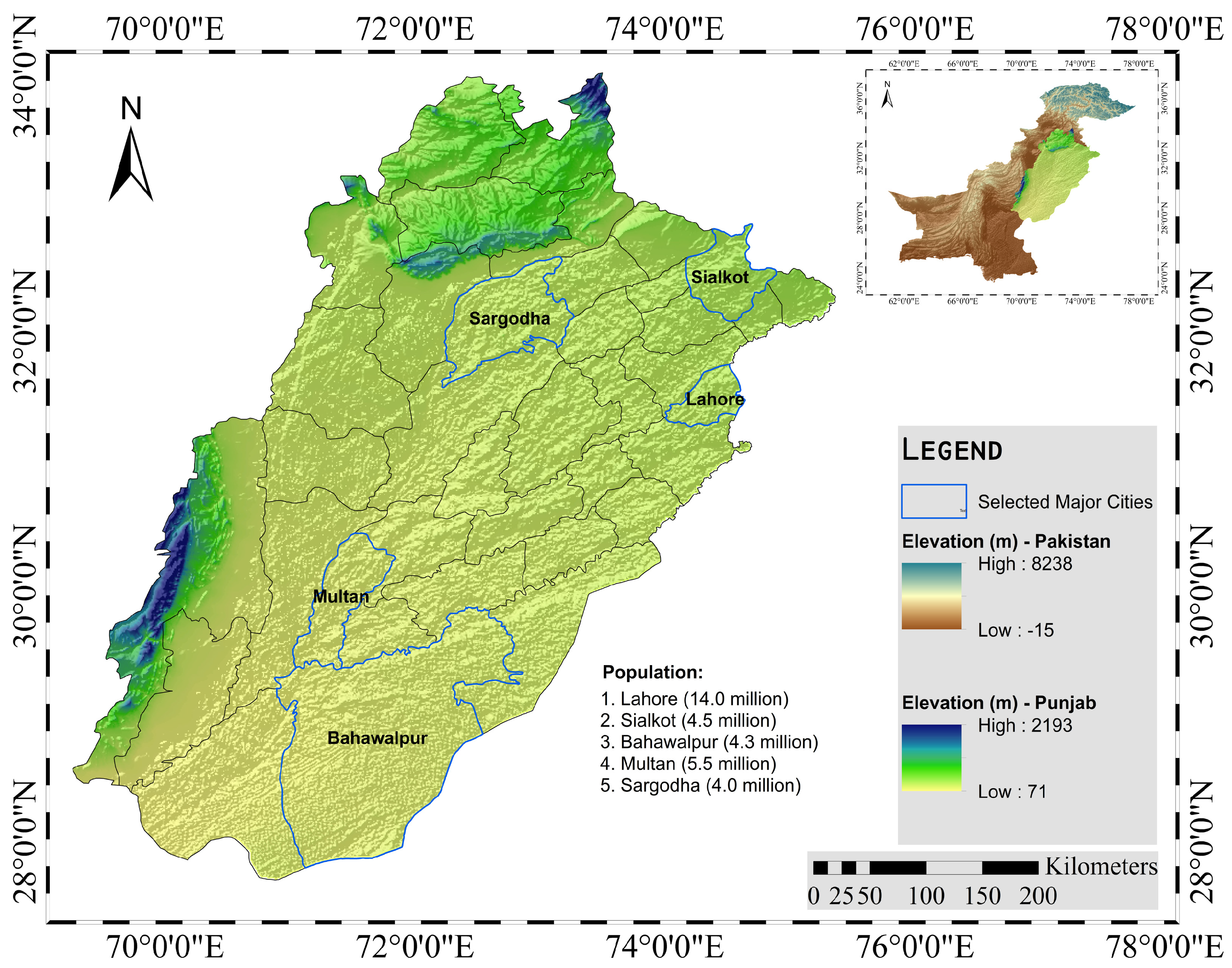
Figure 1. Spatial map of Punjab province (highlighted in green) within Pakistan, overlaid with a Digital Elevation Model (DEM, in meters), illustrating provincial and district boundaries, approximate population distribution, and the locations of the five selected urban centers: Lahore, Sialkot, Multan, Bahawalpur, and Sargodha.
Atmosphere 16 01271 g001
Figure 2. Flowchart for the procedure of generating the updated IDF curves.
Atmosphere 16 01271 g002
Figure 3. Heat map of global climate model ranking for major cities in Punjab.
Atmosphere 16 01271 g003
Figure 4. Taylor diagram of climate model statistical performance for (a) Bahawalpur, (b) Lahore, (c) Multan, (d) Sargodha, and (e) Sialkot.
Atmosphere 16 01271 g004
Figure 5. (a) Comprehensive ranking of GCM models based on their performance in simulating precipitation over major cities of Punjab; (b) Ranked performance of GCMs across the major cities in Punjab.
Atmosphere 16 01271 g005
Figure 6. IDF curves using ground/observed data and historical GCM-simulated data for (a) Bahawalpur, (b) Lahore, (c) Multan, (d) Sargodha, and (e) Sialkot (return period in years).
Atmosphere 16 01271 g006aAtmosphere 16 01271 g006b
Figure 7. Statistical relation between GCM-simulated historical data and ground/observed data to develop the spatially downscaled model output.
Atmosphere 16 01271 g007
Figure 8. Statistical relation between GCM historical and future data to develop the temporally downscaled model output.
Atmosphere 16 01271 g008
Figure 9. Linear relationship derived from the EQM method for spatial downscaling.
Atmosphere 16 01271 g009
Figure 10. Linear relationship derived from the EQM method for temporal downscaling (SSP 2-4.5).
Atmosphere 16 01271 g010
Figure 11. Linear relationship derived from the EQM method for temporal downscaling (SSP 5-8.5).
Atmosphere 16 01271 g011
Figure 12. Updated IDF curves for Lahore city representing the downscaling effect on SSP 2-4.5 for 100-year and 25-year return periods.
Atmosphere 16 01271 g012
Figure 13. Updated IDF curves for Lahore city representing the downscaling effect on SSP 5-8.5 for 100-year and 25-year return periods.
Atmosphere 16 01271 g013
Figure 14. Updated IDF curves for (a) Bahawalpur, (b) Lahore, (c) Multan, (d) Sargodha, and (e) Sialkot.
Atmosphere 16 01271 g014aAtmosphere 16 01271 g014bAtmosphere 16 01271 g014c
Table 1. Recent hazardous rainfall-driven floods in Punjab province.
Extreme Rainfall and FloodsMonth and YearImpact
Heavy flooding due to rainApril 202421 deaths, 5 injuries, significant damage to houses and crops
Catastrophic floodingAugust 2022Over 33 million individuals were affected, with around 1.7 million homes destroyed and close to 1400 lives lost
Monsoon rains and floodingJune–August 2022Widespread flooding, particularly impacting Punjab, Khyber Pakhtunkhwa, Balochistan, and Sindh
Severe floodingSeptember 2014Millions were affected, causing significant damage to infrastructure and agriculture
Heavy monsoon rainsAugust 2011Severe and widespread flooding led to significant loss of life and extensive destruction of property and agricultural land
Massive floodsJuly 2010One of the worst floods in Pakistan’s history, affecting Punjab and other regions, causing massive destruction and loss of life
Table 2. General circulation models (GCMs) used in this research.
Model NameCountryModelling CentreHorizontal Resolution (lon × lat)
BCC-CSM2-MRChinaBeijing Climate Center1.1° × 1.1°
CNRM-CM6-1FranceCentre National de Recherches Météorologiques, Centre Européen de Recherche et de Formation Avancée en Calcul Scientifique1.4° × 1.4°
CNRM-ESM2-1
EC-Earth3-Veg-LREuropeEC-EARTH consortium, published at the Irish Centre for High-End Computing1.1° × 1.1°
HadGEM3-GC31-MMMet Office Hadley Centre0.83° × 0.55°
MIROC6United KingdomAtmosphere and Ocean Research Institute (The University of Tokyo), National Institute for Environmental Studies, and Japan Agency for Marine-Earth Science and Technology1.4° × 1.4°
MRI-ESM2-0JapanMeteorological Research Institute1.1° × 1.1°
Nor-ESM2-MMNorwayBjerknes Centre for Climate Research, Norwegian Meteorological Institute1.25° × 0.9°
Table 3. Test statistics for goodness-of-fit tests.
Goodness-of-Fit TestTest StatisticsDetails
Kolmogorov–Smirnov
(K–S)
S n x = 0 ; i f   X < X 1
S n x = k n ; i f   X k X < X k + 1
S n x = 1 ; i f   X > X n
D n = m a x | F x x S n ( x ) |
P D n D n α = 1 α
Sn(x) = Empirical cumulative frequency
Fx(x) = Cumulative density function of the hypothetical distribution
D n α = Critical value
Anderson–Darling
(A–D)
A 2 = 2 i 1 l n F X x i + ln 1 F X x n + 1 i n n A2 = Quadratic category of EDF
Root Mean Square Error (RMSE) R M S E = 1 n Σ ( x i X ) 2 xi = estimated value
X = recorded data value
Table 4. Goodness of fit test results.
Dataset SourceName of CityBest-Fit Test Statistics ResultHighest Ranked Distribution (Sum of Ranks)
K-S TestA-D TestRMSE Test
Observed DataLahoreLP3 (0.010)GUM (1.888)LP3 (6.202)LP3 (4)
MultanLN2 (0.017)LP3 (0.307)LN2 (1.303)LP3 (6)
BahawalpurLN2 (0.014)LP3 (0.047)LN2 (0.886)LP3 (6)
SargodhaLP3 (0.016)GUM (1.926)LP3 (2.184)LP3 (4)
SialkotLN2 (0.015)LP3 (0.327)LN2 (5.346)LP3 (4)
GCM Historical DataLahoreLN2 (0.021)GUM (0.038)LP3 (2.100)LP3 (5)
MultanLP3 (0.021)GUM (0.029)LP3 (1.768)LP3 (4)
BahawalpurLP3 (0.067)LP3 (0.036)LP3 (7.183)LP3 (3)
SargodhaLP3 (0.024)GUM (0.009)LP3 (1.574)LP3 (4)
SialkotLN2 (0.041)LP3 (0.076)LP3 (4.390)LP3 (5)
GCM Future
(SSP2-4.5)
LahoreLP3 (0.064)LP3 (0.001)LN2 (8.615)LP3 (4)
MultanLP3 (0.035)LP3 (0.002)LP3 (8.123)LP3 (3)
BahawalpurLP3 (0.070)LP3 (0.001)LP3 (8.660)LP3 (3)
SargodhaGUM (0.029)LP3 (0.001)LP3 (3.036)LP3 (5)
SialkotLP3 (0.024)LP3 (0.003)LN2 (5.609)LP3 (4)
GCM Future
(SSP5-8.5)
LahoreLP3 (0.049)LP3 (0.001)LN2 (5.337)LP3 (4)
MultanLP3 (0.068)LP3 (0.011)LP3 (9.486)LP3 (3)
BahawalpurLP3 (0.076)LP3 (0.001)LP3 (13.117)LP3 (3)
SargodhaLP3 (0.070)LP3 (0.003)LN2 (7.450)LP3 (4)
SialkotLP3 (0.041)LP3 (0.004)LN2 (14.292)LP3 (4)
Table 5. Rainfall intensities (mm/hr) for different durations (hours) and return periods (years) estimated using the LP3 distribution for the regions under consideration.
Name of CityDataset SourceReturn Period (Year)Rainfall Duration (hrs)
123461224
BahawalpurObserved Data25.263.452.682.241.741.110.71
512.897.315.294.213.071.821.09
1017.579.686.885.423.902.251.32
2521.8211.838.336.524.642.641.53
5027.0814.5310.177.925.613.161.82
10035.2018.8813.2210.307.294.102.36
GCM Historical Data22.411.941.631.421.150.790.52
57.714.653.482.842.131.310.81
1013.817.785.614.463.251.921.15
2521.1711.568.186.434.602.651.56
5031.0516.6511.669.106.463.662.12
10040.3621.6515.1611.838.394.752.76
GCM Future
(SSP2-4.5)
22.501.601.271.100.900.640.46
510.976.344.633.722.741.640.99
1025.3612.338.666.764.792.701.55
2542.8222.4015.4311.878.254.482.49
5054.5628.3719.4514.9210.325.573.07
10070.9336.8825.2919.4013.427.243.99
GCM Future
(SSP5-8.5)
22.802.001.701.481.240.900.62
513.107.635.604.503.332.001.22
1027.6713.759.737.645.473.131.83
2545.0623.8716.5712.849.015.002.84
5056.8129.8920.6615.9611.156.143.46
10073.8638.8526.8620.7514.497.984.50
LahoreObserved Data229.1518.4714.1311.688.925.633.55
541.5325.8519.6316.1712.307.734.86
1050.2031.0123.4819.3114.679.205.78
2558.6236.0327.2322.3616.9710.636.67
5070.2843.0232.4726.6420.2012.647.93
10091.3655.9342.2134.6326.2516.4310.31
GCM Historical Data223.5014.8511.349.377.164.512.84
533.8320.8315.7512.939.816.143.85
1039.7324.2518.2614.9611.337.074.43
2544.8727.2220.4516.7312.657.884.93
5052.0131.4223.5619.2614.549.055.66
10067.6140.8430.6325.0318.9011.767.36
GCM Future
(SSP2-4.5)
223.6615.3111.819.827.554.803.04
540.6824.6518.4815.1011.397.074.41
1055.8631.6423.4819.0614.268.775.44
2571.2941.4530.4824.6118.2911.166.88
5082.6247.7835.0528.2520.9612.757.85
100107.4162.1245.5636.7227.2516.5810.21
GCM Future
(SSP5-8.5)
226.4917.1113.2010.968.425.353.38
544.4227.2120.5216.8212.737.944.98
1061.7235.3626.4221.5416.2110.046.26
2580.0647.2935.0728.4621.3113.118.14
5093.5054.9740.6732.9724.6415.139.39
100121.5571.4652.8742.8632.0319.6712.20
MultanObserved Data26.704.373.382.822.181.390.89
514.428.306.064.863.572.141.30
1019.2110.757.716.124.442.611.56
2523.5912.989.237.285.233.031.79
5029.1015.8311.198.786.283.602.11
10037.8220.5814.5411.418.164.682.75
GCM Historical Data24.443.042.402.031.591.030.67
512.206.975.064.042.961.761.06
1017.549.676.895.433.912.261.33
2522.6812.288.656.774.822.741.59
5029.1115.5810.898.486.003.371.94
10037.8420.2614.1611.037.804.392.52
GCM Future
(SSP2-4.5)
23.002.001.601.381.120.800.57
511.866.905.064.073.011.811.10
1026.2412.899.097.125.072.881.66
2543.6922.9715.8712.248.544.682.62
5055.4828.9719.9215.3210.635.773.20
10072.1237.6625.9019.9213.827.514.16
GCM Future
(SSP5-8.5)
23.502.401.901.631.340.970.67
512.487.355.424.383.251.971.20
1026.8613.349.467.445.333.051.78
2544.5023.5516.3312.648.864.902.77
5056.4729.6620.4815.8011.016.043.39
10073.4138.5526.6220.5314.327.854.40
SargodhaObserved Data212.027.745.964.953.802.411.53
520.3912.209.097.395.553.422.13
1025.8315.1011.128.996.694.082.52
2530.9317.8213.0310.487.754.692.88
5037.6121.4515.6012.519.225.553.39
10048.8927.8820.2916.2611.987.214.41
GCM Historical Data26.564.403.462.902.261.460.93
514.438.476.255.053.752.281.40
1020.2111.468.306.624.852.891.75
2525.9714.4410.348.205.943.492.09
5033.3418.3013.0110.267.404.302.56
10043.3423.7916.9213.349.615.593.32
GCM Future
(SSP2-4.5)
27.715.204.093.442.681.741.12
522.3412.589.067.205.233.071.83
1033.9217.5212.389.716.933.952.30
2544.9323.9816.7313.009.165.112.91
5052.5127.8719.3715.0210.545.853.32
10068.2736.2425.1819.5213.717.604.31
GCM Future
(SSP5-8.5)
29.606.695.334.513.552.321.50
523.8814.1110.448.456.303.842.37
1038.4920.4414.7911.818.645.143.11
2554.4429.9921.3716.8812.187.104.23
5065.4935.8225.4220.0214.408.354.95
10085.1446.5733.0426.0218.7110.856.43
SialkotObserved Data224.8515.7612.069.977.624.813.03
536.1622.3916.9613.9510.606.654.18
1043.6026.7420.1916.5612.567.854.93
2550.6030.8423.2219.0314.408.995.64
5060.2136.5327.4522.4716.9910.596.64
10078.2847.4935.6929.2122.0813.778.63
GCM Historical Data220.8813.2310.128.376.404.042.54
531.6319.4614.7112.079.165.733.60
1038.2223.2817.5214.3510.856.774.24
2544.1926.7420.0716.4112.397.714.82
5052.2731.4823.5719.2514.529.025.64
10067.9640.9330.6525.0318.8711.737.33
GCM Future
(SSP2-4.5)
221.8114.0510.838.996.914.392.78
537.8722.6316.8613.7110.286.333.93
1050.8528.4820.9616.9312.587.664.72
2563.3336.2426.4121.1915.639.425.76
5072.5941.3130.0224.0417.6910.636.49
10094.3753.7039.0231.2523.0013.828.43
GCM Future
(SSP5-8.5)
220.9413.7610.698.926.884.402.80
536.2122.0516.5813.5610.246.373.98
1052.2629.3221.7317.6313.188.095.02
2570.0340.4429.6323.8617.6810.746.60
5082.8847.5434.7127.9020.6212.487.66
100107.7461.8045.1336.2726.8116.229.96
Table 6. Empirical formulas of the selected probability distribution intended for all major cities in Punjab, corresponding to different data sources.
Name of CityDataset Source
Observed DataGCM HistoricalGCM Future
(SSP2-4.5)
GCM Future
(SSP5-8.5)
Bahawalpur i = 5.15 T 0.440 t 0.797 i = 2.11 T 0.688 t 0.746 i = 2.40 T 0.814 t 0.822 i = 2.83 T 0.785 t 0.788
R2 = 0.9180R2 = 0.9448R2 = 0.9041R2 = 0.8931
Lahore i = 25.42 T 0.272 t 0.680 i = 21.23 T 0.245 t 0.690 i = 21.10 T 0.364 t 0.719 i = 23.16 T 0.371 t 0.706
R2 = 0.9839R2 = 0.9696R2 = 0.9660R2 = 0.9725
Multan i = 6.37 T 0.403 t 0.778 i = 4.35 T 0.500 t 0.789 i = 2.82 T 0.776 t 0.811 i = 3.21 T 0.747 t 0.798
R2 = 0.9353R2 = 0.9178R2 = 0.9111R2 = 0.9196
Sargodha i = 10.83 T 0.331 t 0.729 i = 6.01 T 0.448 t 0.758 i = 7.86 T 0.507 t 0.811 i = 8.90 T 0.526 t 0.759
R2 = 0.9670R2 = 0.9490R2 = 0.8945R2 = 0.9335
Sialkot i = 21.95 T 0.271 t 0.686 i = 18.75 T 0.276 t 0.691 i = 19.86 T 0.349 t 0.734 i = 18.05 T 0.402 t 0.721
R2 = 0.9796R2 = 0.9724R2 = 0.9588R2 = 0.9728
Table 7. Updated IDF curves and the relative percentage changes in intensities for future climate scenarios in the regions under consideration.
Name of CityScenarioDataset SourceReturn Period
25102550100
BahawalpurHistoricalObserved Data5.2612.8917.5721.8227.0835.20
SSP2-4.5GCM Future2.5010.9725.3642.8254.5670.93
Downscaled GCM Future2.4011.0625.3642.7054.3870.69
Change in % to observed−54.37%−14.16%44.31%95.72%100.80%100.80%
% effect of Downscaling−4.00%0.84%0.00%−0.27%−0.33%−0.33%
SSP5-8.5GCM Future2.8013.1027.6745.0656.8173.86
Downscaled GCM Future3.0013.5528.1145.4957.2574.42
Change in % to observed−42.97%5.14%59.95%108.5%111.39%111.39%
% effect of Downscaling7.14%3.44%1.58%0.93%0.76%0.76%
LahoreHistoricalObserved Data29.1541.5350.2058.6270.2891.36
SSP2-4.5GCM Future23.6640.6855.8671.2982.62107.41
Downscaled GCM Future25.7442.9858.3674.0085.57111.24
Change in % to observed−11.70%3.48%16.26%26.23%21.76%21.76%
% effect of Downscaling8.76%5.65%4.48%3.80%3.56%3.56%
SSP5-8.5GCM Future26.4944.4261.7280.0693.50121.55
Downscaled GCM Future32.3851.2869.5188.84103.23134.20
Change in % to observed11.11%23.47%38.48%51.56%46.89%46.89%
% effect of Downscaling22.27%15.45%12.63%10.97%10.40%10.40%
MultanHistoricalObserved Data6.7014.4219.2123.5929.1037.82
SSP2-4.5GCM Future4.849.8516.8634.3358.78100.65
Downscaled GCM Future3.5012.3426.6644.0455.8172.55
Change in % to observed−47.76%−14.42%38.77%86.69%91.80%91.80%
% effect of Downscaling−27.64%25.31%58.12%28.30%−5.06%−27.92%
SSP5-8.5GCM Future3.5012.4826.8644.5056.4773.41
Downscaled GCM Future3.6013.6728.0745.7557.8075.15
Change in % to observed−46.27%−5.22%46.11%93.91%98.67%98.67%
% effect of Downscaling2.86%9.47%4.51%2.81%2.36%2.36%
SargodhaHistoricalObserved Data12.0220.3925.8330.9337.6148.89
SSP2-4.5GCM Future7.7122.3433.9244.9352.5168.27
Downscaled GCM Future9.3824.0335.6246.6554.3370.62
Change in % to observed−22.00%17.84%37.91%50.83%44.45%44.45%
% effect of Downscaling21.63%7.56%5.03%3.83%3.46%3.46%
SSP5-8.5GCM Future9.6023.8838.4954.4465.4985.14
Downscaled GCM Future13.8428.6143.7360.2371.8693.42
Change in % to observed15.08%40.32%69.27%94.74%91.08%91.08%
% effect of Downscaling44.14%19.82%13.62%10.64%9.73%9.73%
SialkotHistoricalObserved Data24.8536.1643.6050.6060.2178.28
SSP2-4.5GCM Future21.8137.8750.8563.3372.5994.37
Downscaled GCM Future23.0439.2352.3264.9174.3096.59
Change in % to observed−7.29%8.48%20.00%28.27%23.39%23.39%
% effect of Downscaling5.65%3.60%2.89%2.49%2.35%2.35%
SSP5-8.5GCM Future20.9436.2152.2670.0382.88107.74
Downscaled GCM Future24.0639.7756.3074.5987.94114.32
Change in % to observed−3.20%9.98%29.13%47.40%46.04%46.04%
% effect of Downscaling14.89%9.85%7.73%6.51%6.11%6.11%
Table 8. Updated empirical formulas of the selected probability distribution for downscaled GCM future projections.
Name of City Dataset Source
Observed DataGCM Future
(SSP2-4.5)
Downscaled GCM Future (SSP2-4.5)GCM Future
(SSP5-8.5)
Downscaled GCM Future (SSP5-8.5)
Bahawalpur i = 5.15 T 0.440 t 0.797 i = 2.40 T 0.814 t 0.822 i = 2.35 T 0.820 t 0.819 i = 2.83 T 0.785 t 0.788 i = 3.02 T 0.770 t 0.783
R2 = 0.9180R2 = 0.9041R2 = 0.900R2 = 0.8931R2 = 0.895
Lahore i = 25.42 T 0.272 t 0.680 i = 21.10 T 0.364 t 0.719 i = 22.85 T 0.353 t 0.715 i = 23.16 T 0.371 t 0.706 i = 28.13 T 0.346 t 0.699
R2 = 0.9839R2 = 0.9660R2 = 0.984R2 = 0.9725R2 = 0.978
Multan i = 6.37 T 0.403 t 0.778 i = 2.82 T 0.776 t 0.811 i = 3.20 T 0.744 t 0.811 i = 3.21 T 0.747 t 0.798 i = 3.42 T 0.738 t 0.777
R2 = 0.9353R2 = 0.9111R2 = 0.920R2 = 0.9196R2 = 0.912
Sargodha i = 10.83 T 0.331 t 0.729 i = 7.86 T 0.507 t 0.811 i = 9.28 T 0.472 t 0.801 i = 8.90 T 0.526 t 0.759 i = 12.35 T 0.464 t 0.741
R2 = 0.9670R2 = 0.8945R2 = 0.909R2 = 0.9335R2 = 0.953
Sialkot i = 21.95 T 0.271 t 0.686 i = 19.86 T 0.349 t 0.734 i = 20.91 T 0.341 t 0.731 i = 18.05 T 0.402 t 0.721 i = 20.63 T 0.383 t 0.714
R2 = 0.9796R2 = 0.9588R2 = 0.961R2 = 0.9728R2 = 0.977
Disclaimer/Publisher’s Note: The statements, opinions and data contained in all publications are solely those of the individual author(s) and contributor(s) and not of MDPI and/or the editor(s). MDPI and/or the editor(s) disclaim responsibility for any injury to people or property resulting from any ideas, methods, instructions or products referred to in the content.