Abstract
Microplastics (MPs) are emerging pollutants detected in diverse environments and human tissues. Among them, airborne MPs (AMPs) remain poorly characterized due to limited data and methodological inconsistencies. Although regarded as analogous to particulate matter (PM), detailed comparisons with its components are scarce. To address this gap, this study implemented a unified and seasonal protocol for simultaneous measurement of AMPs and PM across three sites in Japan. AMPs were identified using micro-Raman spectroscopy, enabling polymer- and morphology-resolved analysis. A total of 106 AMPs were identified across all sites and seasons. Polyethylene (PE) was consistently dominant, followed by polyethylene terephthalate (PET) and polyamide (PA). Site-specific variation was evident, with certain polymers being relatively more abundant depending on the local environment. Feret diameter analysis showed a modal range of 4–6 μm, with fragments predominating over granular and fibrous particles. Significant correlations between AMP concentrations and PM components were determined, including syringaldehyde (SYAL), tungsten (W), cobalt (Co), and chromium (Cr), suggesting links to local sources, while indicating that AMP dynamics are not always aligned with PM behavior. This study provides one of the first integrated datasets of AMPs and PM components, offering insights into their occurrence, sources, and atmospheric relevance.
1. Introduction
Plastic products have brought benefits to humanity from their inception to the present day. On the other hand, with the World Economic Forum estimating that approximately 8 million tons of plastic waste is dumped into the oceans every year [1], the problem of plastic waste has become an urgent issue. Microplastics (MPs) are defined as synthetic plastic particles usually less than 5 mm in diameter [2]. It is estimated that there are more than 5 trillion MPs in the world’s oceans [3], and they are reported to be distributed vertically not only in the surface but also in deeper layers in the ocean [4]. Moreover, MPs have been detected globally in other environments, such as river [5,6], lake [7], soil [8,9], vegetation [10], wildlife animals [11], and air [12,13,14,15,16,17], which may suggest that MPs are ubiquitous on Earth. Furthermore, the presence of MPs in various bodily fluids and tissues, including the lungs [18,19], breast milk [20], placenta [21], and blood [22], has been documented. These observations have led to concerns regarding potential adverse health implications, such as an increased risk of heart disease [21], and cellular and DNA damage [23]. Consequently, MPs have emerged as a pervasive social problem on a global scale, underscoring the imperative for the promotion of research in this domain.
The initial detection of Airborne Microplastics (AMPs) was documented in 2016 [24], a comparatively late occurrence in the context of other environmental contaminants. Since then, the presence of AMPs has been documented globally in both urban [25,26,27,28] and mountainous regions [13,15,16,29]. A circulation model analogous to that of other air pollutants has been developed, in which AMPs are transported from their sources, persist in the atmosphere, and are deposited on the ground surface through a scavenging effect during precipitation [30,31]. The aforementioned definition of AMPs as fine plastic fragments (solids) measuring 5 mm or less, along with their inhalability, underlines the potential for AMPs to be classified as a type of Particulate Matter (PM) or to be found within PM [30,32]. On the other hand, reported cases of AMPs are limited in the overall MPs research [16,17]: Of all MPs studies, only about 13% (about 20 cases) of AMPs related studies were reported in 2021 [30]. In addition, the mix of sample collection, preparation, and plastic identification methods used to measure AMPs makes it difficult to compare data from different methods. For example, although all measured AMPs in the previous studies compared by Revell et al. were limited to active sampling, their atmospheric concentration equivalents varied from 0.01 to 5650 MP m−3, a difference of six orders of magnitude [33], suggesting that the influence of inter-method error cannot be ignored even when considering concentration differences between sampling sites [17]. Therefore, it is imperative to employ the unified method for meticulous measurement in order to comprehensively grasp the dynamics and the fate of AMPs, in addition to conducting risk assessments.
Identification of the source of AMPs is another important issue to solve as plastic products and waste are widespread on Earth. The potential sources of these emissions are diverse and include, but are not limited to, automobile emissions, sea spray, waste disposal facilities, agricultural activities, soil re-scattering, urban dust, industry, and long-range transport [14,28,31,34,35,36,37]. Brahney et al. presented model estimates indicating that 84% of AMPs over the western United States originate from road and braking emissions, also concluding that this can vary depending on various factors, including location and land use [37]. Despite the evident similarity to PM mentioned above, the attempts to employ tracer components of PM to ascertain the source of AMPs have been constrained. Akhbarizadeh et al. were the first to seek a relationship between AMPs and Polycyclic Aromatic Hydrocarbons (PAHs) contained in PM [38], and Kirchsteiger et al. demonstrated a robust correlation between AMPs and single PAH congeners [39]. To the best of our knowledge, however, no studies have been reported that focus on the clear correlation between AMPs and PM tracer components, including ions, metals, and organic components other than PAHs.
Considering the aforementioned background of research in this domain, this study presents the results of AMP measurements (e.g., number concentration, polymer type, and particle size) for each sampling site obtained using unified sample collection, preparation, and identification methods throughout the study. These measurements were based on seasonal intensive observations at multiple sampling sites in Japan, each of which exhibited distinctive characteristics. Furthermore, an attempt was made to obtain information that would contribute to the identification of the source of AMPs from the strength of correlation with each component of PM measured simultaneously, combining with comparison with meteorological data and backward trajectory analysis. The results of this study were reported in the following sections.
2. Materials and Methods
2.1. Sample Collection
2.1.1. Sampling Sites and Attributes
Observations were conducted at three sites in Japan: Kawasaki (urban), Niigata-sowa (semi-urban), and Kasahori Dam (rural). Their attributes were classified referring to the EANET technical manual [40]. Urban sites are influenced by traffic, residential and industrial activities, while the rural site is surrounded by forests, agricultural land, and a reservoir. Niigata-sowa and Kawasaki are located within 3 km of the coast, whereas Kasahori Dam is inland. A map and site satellite images were shown in Figure 1. Table A1 provides additional details on surrounding environments.
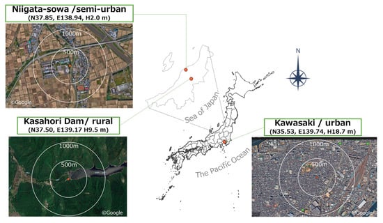
Figure 1.
The names, attributes, locations (specifically, longitude, latitude, and collection surface height above ground), and satellite images of each sampling site.
2.1.2. Sampling Methods
At each site, AMPs were collected as total suspended particles (TSPs) on PTFE filters, while PM was collected on quartz fiber filters using a cascade impactor to separate fine (PM2.5) and coarse particles larger than 2.5 μm in diameter (hereinafter referred to as “PMc”). The primary objective of the PM size classification was to enable comparison and interpretation, given the recognized bias toward coarse and fine PM with respect to specific components and the fact that previous studies on tracer components have predominantly focused on PM2.5 [41,42,43,44,45]. Filters were housed in metal windshields and operated with low-volume pumps (10 L/min (converted to 20 °C), 6–8 days per sample; ≥70 m3 per sample to avoid possible contamination [46]). The observation campaigns were conducted seasonally at the three sites from November 2023 to October 2024. Each campaign lasted approximately one month per season, during which both AMP and PM samples were collected simultaneously. In total, 16 valid samples were obtained per site (four per season). Sampling was conducted continuously without major interruptions or instrument downtime, except for a short-term power outage at the Kawasaki site between April 2 and 10, 2024, which resulted in the exclusion of one PM sample due to incomplete data acquisition. Accordingly, the datasets represent typical seasonal conditions of the respective locations. The detailed schedule of sampling periods is summarized in Table A6. The overall sampling system was illustrated in Figure 2. Collected PTFE filters were dried in a desiccator (<30% RH) prior to preparation (Section 2.2). Quartz fiber filters were stored frozen (−4 °C) until analysis of ions, elements, and organics (Section 2.3). Detailed procedures are delineated in Appendix B.1.1.
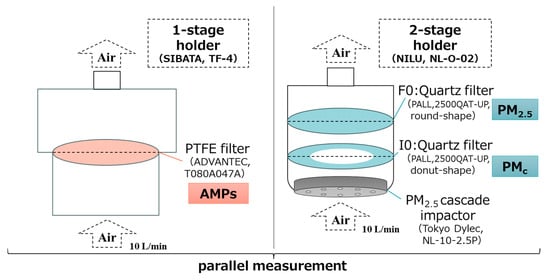
Figure 2.
A schematic diagram illustrating the filter papers and their holders utilized for parallel measurements, as well as the substances intended for collection, respectively. The definition of PMc was delineated in Section 2.1.2.
2.2. AMPs Sample Preparation and Identification
2.2.1. Preparation for AMPs Samples
Samples were processed in a clean room to minimize contamination. Preparation followed a three-step procedure widely adopted in previous studies [5,17,28,47]: (i) organic matter removal by H2O2 treatment, (ii) density separation using NaI solution, and (iii) centrifugation. The final extracts were filtered onto alumina filters (φ25 mm, pore size 0.2 µm), concentrating the effective area to φ4 mm. The procedure was summarized in Figure 3. Appendix B.1.2 provides additional experimental details.
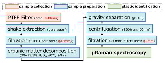
Figure 3.
A flow diagram delineating the outline protocol for preparation of AMP samples.
2.2.2. Identification of AMPs
Polymer identification was performed using µRaman spectroscopy (JASCO NRS-4500), renowned for its high spatial resolution and sensitivity [48]. Measurement conditions were optimized to minimize sample damage and fluorescence interference (Table 1), while it remained challenging to entirely mitigate these risks [17,38,49,50,51]. Thirty fields of view (100× lens) were randomly selected per sample. All particles showing C–H stretching bands (2800–3000 cm−1) were analyzed. Raman spectra (500–3600 cm−1) were compared with a spectral library (KnowItAll, Wiley), and particles with HQI ≥ 75 as the top match were classified as plastics. “HQI (Hit Quality Index)” is a metric of spectral consistency, with 100 representing a perfect match and 0 representing a complete mismatch. Particle size was also measured. Although the spatial resolution of the μRaman utilized in this study is not specified by the manufacturer, it is generally accepted to be approximately 1 μm for models with standard specifications [38], with the exception of high-end configurations [50,52]. Given that the pore size of the filter paper used for AMPs collection was 0.8 μm and the minimum Feret diameter of the identified AMPs exceeded 1 μm, this study focused on AMPs larger than 1 μm in Feret diameter. All reported particle sizes represent geometric diameters derived from image analysis and are not directly equivalent to aerodynamic diameters, particularly for irregular, low-density plastic particles. Because the measurement was based solely on the optical projection of TSP-collected particles, conversion to aerodynamic diameter is not possible from the current dataset without additional information on particle density, shape, and dynamic shape factors. According to the WHO guideline and previous studies [53,54], morphology was determined as follows: fibers are particles with an aspect ratio of Feret diameter to short diameter greater than 3:1; granules are those with an aspect ratio less than 1.2:1; fragments are those with an aspect ratio between the two categories. The number concentration of AMPs was calculated using the following Equation (1):
and the following is a list of the meanings of the parameters indicated by each symbol.
- C: The number concentration of AMPs [MPs m−3];
- n: The number of AMPs identified [MPs];
- Sf: The effective filtration area (= φ4 mm) [m2];
- V: The total air suction amount (converted to 20 °C) [m3];
- Sr: The area of a field of view of μRaman (=140 μm × 110 μm) [m2];
- N: The number of fields of view of μRaman measured (=30).

Table 1.
The measurement conditions and settings of μRaman in this study.
Table 1.
The measurement conditions and settings of μRaman in this study.
| Items | Conditions/Settings |
|---|---|
| measurement mode | single point measurement |
| visual field image mode | mixture of dark/bright |
| range of targeted wavenumbers | 500−3600 cm−1 |
| accumulation count | 3−5 times |
| exposure time | 5−10 s/time |
| excitation wavelength | 532 nm (green) |
| maximum laser power | 50 mW |
| laser power output | 1−5% of the maximum |
| slit type | φ100 μm, φ34 μm, φ17 μm |
| grating type | 900 line/mm |
QA/QC included blanks and recovery tests demonstrated by a previous study [17]. Appendix B.1.3 provided additional experimental details.
2.3. PM Samples Preparation and Analysis
Quartz fiber filters were quartered and allocated to ion, element, or organic analysis following national manuals and prior studies [45,55,56,57,58]. Ions were analyzed by ion chromatography, inorganic elements by ICP-MS, and organics by GC/MS. Analytical conditions and abbreviations are provided in Table A2 and Table A3. Comprehensive procedures, reagents, equipment, storage methods, and QA/QC protocols were delineated in Appendix B.1.4.
2.4. Data Analysis
2.4.1. Simple Pearson Regression Analysis
Simple Pearson regression analyses to evaluate the linear relationship were performed for each location, with the number concentration of AMPs serving as the response variable and the PM2.5 components and meteorological parameters (i.e., averaged wind speed, maximum instantaneous wind speed, and averaged precipitation) serving as the explanatory variables. Consequently, the explanatory variables employed in this study amounted to 52, encompassing PM2.5 components and meteorological parameters. The rationale behind the exclusive focus on PM2.5 as a target for PM tracer components was elucidated in Section 2.1.2. The meteorological data from the nearest stations (AMeDAS) whose data were available to the sampling sites were used for analysis [59]. However, in the case of Kasahori Dam, meteorological instruments were installed at the sampling site, and the data from these instruments were utilized. Satellite images which delineate Niigata-sowa and Kawasaki as well as the nearest AMeDAS to each of the sampling sites, namely Maki and Haneda, are shown in Figure A1.
2.4.2. Back-Trajectory Clustering
The calculation of back trajectories was performed using meteorological data (CFSv2, time resolution: 3 h, spatial resolution: 0.5 × 0.5 degree) from the National Centers for Environmental Prediction (NCEP) via the online software METEX [60,61]. The trajectories were calculated at 8-h intervals under the 3D-wind (kinematic) mode, with a 7-day trajectory length from the receptor sites, corresponding to three sampling sites delineated in Section 2.1.1. The altitude of all the receptor sites was set at 500 m. Although the temporal resolution of the METEX trajectories may be relatively coarse, the purpose of this study was not to interpret individual trajectories in detail but to capture representative transport patterns at a regional scale. By applying cluster analysis, the uncertainties of individual trajectories are averaged out, allowing for the analysis of large-scale horizontal transport pathways. The following procedures for trajectory clustering, including preprocessing the output csv files from METEX and ratio aggregation, were implemented in Python (v3.11) and executed in Google Colab. The trajectories of each receptor site were allocated to discrete clusters in accordance with their velocity and trajectory, employing Ward’s hierarchical method, which is predicated on the Euclidean distance between all possible pairs of trajectories. This clustering approach was applied to group similar trajectories into representative patterns, thereby reducing noise from individual trajectory uncertainties and highlighting large-scale transport features. Ward’s hierarchical method was selected because it minimizes within-cluster variance and has been widely applied in trajectory studies for regional-scale source identification [16,62,63]. The representativeness of each cluster facilitates the interpretation of long-range transport pathways and their potential influence on receptor sites, rather than focusing on single trajectories that may be affected by model uncertainty. The outcomes of the hierarchical clustering algorithm are contingent upon the number of clusters. In this study, the final number of clusters at all receptor sites was determined to be four, based on the variation of total spatial variance (TSV) with cluster numbers (see Figure A2).
3. Results and Discussion
3.1. Comparative Overview of AMPs and Major PM Components
Table 2 presents the annual average values of the AMP number concentrations and the total ion mass concentrations of PM2.5 and PMc for each sampling site. As stated in the previous studies, soluble inorganic ions have been found to comprise as much as 60–70% of the total mass of suspended particulate matter [64], and 30–50% of the total PM2.5 mass [65,66]. Given that ion components are widely regarded as the predominant constituents of PM, ion mass concentrations were utilized as metrics to comparatively analyze AMPs and PM. A comparison with the results of previous studies that also employed the active sampling method revealed that the AMPs number concentrations ranged from 0.01 to 5650 MP m−3 (N = 13, median: 2.9 MP m−3) [12,14,26,33,38,54,67,68,69,70]. Notably, the results for all three locations fell within this range, indicating a consistency in the findings across different study sites. Focusing on the comparison of concentrations between PM and AMPs, the concentrations were Kawasaki, Niigata-sowa, and Kasahori Dam in descending order, a commonality observed across all three items (i.e., AMPs, PM2.5, and PMc). While the concentration differences among the three sites proved to be statistically significant for both PM2.5 and PMc (N = 15 for Kawasaki, N = 16 for the other two sites, p < 0.05), no significant differences were detected in the AMPs number concentration (N = 16 each, p > 0.05). Weekly fluctuations of AMPs number concentrations, ion mass concentrations of PM2.5/PMc, and the predominant wind directions at each sampling site were delineated in Figure A3. Although seasonal fluctuation was observed, PM2.5 tended to have a relatively high proportion of SO42− and NH4, while PMc tended to have a relatively high proportion of Cl−, Na+, and Ca2+ regardless of the locations, which is consistent with previous studies [58,64,65,66]. However, no clear correlation was observed between total ion mass concentration of PM2.5/PMc and AMP number concentration at any location. According to the Japan Meteorological Agency, dust and sandstorms (DSS) originating from mainland China were observed during 5–12 December 2023 and 16–23 April 2024, respectively [71]. While the PMc mass concentration of Ca2+, which is known as part of the major components of DSS, was relatively elevated at three sampling sites, there was no significant increase in the number concentration of AMPs during both periods.
Table 2.
Annual average values of AMPs. Number (No.), concentration (conc.), and PM2.5/PMc total ion mass conc. at each site.
In the context of PM source analysis, the concentrations and ratios of inorganic elements have been employed, which are less susceptible to compositional changes by chemical reactions during long-term transportation in the atmosphere [72]. Taniguchi et al. directed their attention to the ratio of Pb mass concentration in fine particles to that of Cu in coarse particles (Pb/Cu), reporting the efficacy of Pb/Cu as an indicator of transboundary and local air pollution, with a particular emphasis on the emissions from coal combustion and motor vehicle traffic, respectively [57]. In this study, the mass concentration ratio of Pb in PM2.5 to Cu in PMc (Pb2.5/Cuc) was utilized, and the values for each sampling site were displayed in Figure 4 as box and whisker plots. The mean Pb2.5/Cuc values at the three sampling sites were highest at Kasahori Dam, followed by Niigata-sowa and Kawasaki. Furthermore, statistically significant differences in the mean Pb2.5/Cuc values were observed among the three sites (p < 0.05 or p < 0.01). This tendency for Pb/Cu values to be higher in rural areas and lower in urban areas has been reported in a previous study and is consistent with the results of this study [57].
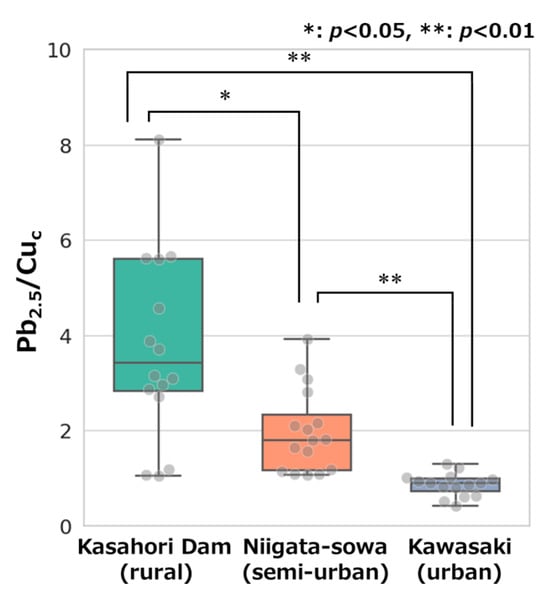
Figure 4.
Box and whisker plots of the mass concentration ratio of Pb in PM2.5 to Cu in PMc (Pb2.5/Cuc) at each site. An outlier is observed with a value of 15.6 for Kasahori Dam.
In consideration of the findings, the conditions of air pollution, as indicated by the ion mass concentrations—the primary constituent of PM—and the indicator defined by the mass concentration ratio of inorganic elements, were found to be generally consistent with the attributes assigned to each location. In contrast, the relationships between AMP number concentrations and site attributes were unclear. Therefore, it was hypothesized that there might be little correlation between AMPs concentrations and conventional site attributes defined by the concentration level of air pollutants like PM on a macroscopic level, suggesting that AMPs pollution may be occurring at the same level in rural, semi-urban, and urban areas. It was also indicated that AMP dynamics are influenced by additional factors beyond conventional particulate matter processes, and may not be directly inferred from PM behavior alone.
3.2. Composition, Size, and Morphology of AMPs
3.2.1. Polymer Composition of AMPs
Breakdowns of AMP polymer types for the total and individual sampling sites were presented in Figure 5. In addition, the original names and their acronyms for the AMP polymer types identified in this study were delineated in Table A4. A total of 106 AMPs were identified at the three locations throughout all the sampling periods, with PE (39.6%) being the most common polymer type, followed by PET (10.4%), PA (9.4%), and PS (8.5%) in a descending order. The AMPs identified in this study were all general-purpose polymers, most of which have been previously reported in other studies [33]. PE was also the most frequently detected polymer type at each location, accounting for 30.0–46.7% of the total. PE is among the most widely utilized plastics on a global scale, and this is primarily due to its high density, chemical and temperature resistance, and versatility in a variety of applications [73,74]. The predominance of PE in AMPs was also consistent with the estimation of the previous survey, which indicated that PE accounted for 33.8% of the total plastic waste and 23.4% of the total plastic production in Japan in 2021 [75].
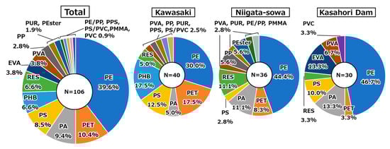
Figure 5.
Breakdowns of AMP polymer types for the total and individual sampling sites. Acronyms were delineated in Table A4.
An analysis of each location reveals the predominance of PET and PHB in Kawasaki, RES in Niigata-sowa, and EVA in Kasahori, respectively. According to the findings of a preceding study, PET had been demonstrated to comprise a substantial percentage of MPs in urban dust at major cities in China [25]. In this study, the proportion of PET was highest in Kawasaki (17.5%), which exhibits the strongest urban characteristics among the three sampling sites, followed by Niigata-sowa (8.3%) and Kasahori Dam (3.3%). Consequently, it was suggested that the proportion of PET could be influenced by the extent to which the given location exhibits characteristics of an urban environment. Regarding PHB, to the best of our knowledge, this study is the first to report detecting PHB as AMP. Figure A4 delineated Raman spectra of polyhydroxybutyrate (PHB) from the KnowItAll library (orange, top row) and the identified AMP (black, bottom row), along with an actual field-of-view image of the AMP. PHB is classified as a type of biodegradable plastic that has garnered attention as a potential substitute for conventional non-biodegradable plastics [76]. The preceding study demonstrated that the half-life of a film of PHB with a thickness of 85 μm on the seafloor ranged from 54 days to 1247 days, while no degradation was observed for a low-density PE film under the same condition [77]. However, previous experiments simulating real environments confirmed that primary PHB particles underwent abiotic degradation to produce secondary MPs, which had a negative impact on water organisms [78]. In light of these findings and considerations, it was suggested that secondary MPs may be dispersed into the atmosphere as a result of PHB degradation in the ocean or other environments. It is also noteworthy that PHB detection was limited to Kawasaki. While there is a possibility that this discrepancy may be indicative of variations in environmental conditions, a definitive correlation with meteorological factors (i.e., averaged wind speed, maximum instantaneous wind speed, and averaged precipitation) remains elusive. RES, which is referring to epoxy and phenoxy resins, has been widely used for coatings, electronic materials, adhesives, and matrices for fiber-reinforced composites [79]. EVA has been widely used in the footwear industry for insoles, midsoles, and outsoles as well as in the wire and cable industry for heat shrinkable insulation, semi-conductive jackets, and flame-retardant coatings [80,81]. Given the general-purpose nature of both polymers, it is challenging to ascertain the origin of AMPs. Although it is noteworthy that EVA was detected exclusively at Kasahori Dam, correlations with the aforementioned meteorological factors were not significant (p > 0.05).
In consideration of the aforementioned factors, it was postulated that the polymer composition offered partial insight into the source and the environmental context. However, it is also imperative to acknowledge the limitations inherent in evaluating the composition in isolation.
3.2.2. Feret Diameter Distribution and Morphological Classification of AMPs
The mean Feret diameter was 10.9 ± 10.6 μm across all locations, 9.1 ± 6.2 μm in Niigata-sowa, 12.9 ± 15.2 μm in Kawasaki, and 10.5 ± 5.7 μm in Kasahori Dam, respectively. As illustrated in Figure 6, the histograms delineated the Feret diameter of AMPs for the total and individual sampling sites. A cross-site examination revealed that the most prevalent size class was 4–6 μm, with the tiny AMPs measuring below 10 μm constituting 66.0% (N = 70) of the total. Revell et al. reported a typical distribution between 15 and 250 μm under the various preparation and identification methods, which was larger than the particle size distribution in this study [33]. Conversely, Levermore et al. reported that the 5 to 10 μm class accounted for 52.5% and the 11 to 20 μm class accounted for 35.0% of the particles identified using μRaman for AMPs [67]. Likewise, Sasaki et al. reported a comparable tendency in their findings, noting that the mean of the calculated aerodynamic equivalent diameter of AMPs was 7.6 ± 3.7 μm [17]. These results both based on μRaman identification indicated a smaller particle size distribution, which was consistent with the present study. In general, the spatial resolution of μRaman is approximately 1 μm, which is sufficiently appropriate to capture tiny AMPs. Consequently, it was hypothesized that discrepancies in identification methodologies resulted in variations in the size distribution of particles between the studies. A comparison of the locations revealed divergent results for the most prevalent values, with Niigata-sowa and Kawasaki demonstrating 4–6 μm, while Kasahori Dam exhibited 6–8 μm and 8–10 μm. Furthermore, Kawasaki exhibited a relatively broad particle size distribution, ranging from 1.4 to 79.8 µm, with the smallest particle size being 1.4 µm, which approaches the detection limit of μRaman. In addition, particles larger than 30 µm, which were not detected in the other two locations, were confirmed. The observed discrepancy in the size distribution of particles can be attributed to variations in environmental conditions across different locations. It was suggested that these cross-site variations were particularly attributable to the generation from the source and the processes of micro-fragmentation induced by subsequent degradation of AMPs, while the limited number of samples made it difficult to draw clear conclusions.
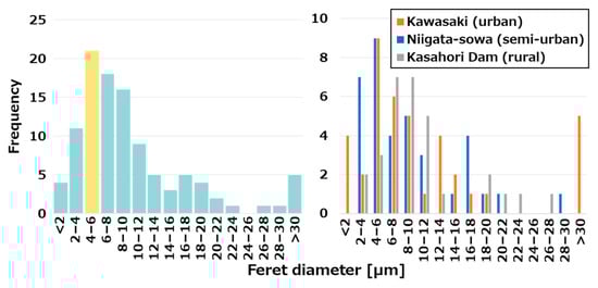
Figure 6.
Histograms of the Feret diameter of AMPs for the total and individual sampling sites.
Breakdowns of AMP morphologies (fragment, granule and fiber) for the total and individual sampling sites were presented in Figure A5. The distinction between fragments, granules, and fibers was made according to the definition of aspect ratio shown in Section 2.2.2. A cross-site analysis revealed that fragmented AMPs were the most prevalent (57.5%), followed by granular (35.8%) and fibrous AMPs (6.6%). This tendency was observed in each of the three locations: Kawasaki, Niigata-sowa, and Kasahori Dam. The results of this study indicated minimal variation in the morphology of AMPs across different locations, suggesting that other factors may be more significant in determining their characteristics. Previous AMPs studies have broadly classified these into two categories: those with a high proportion of fibers [25,27,69] and those with a high proportion of particles and fragments [13,17,38,82]. It was pointed out that this tendency may be contingent upon the preparation method utilized, in particular, some previous studies demonstrated that particles and fragments prevail when employing both the organic decomposition and the heavy liquid (gravity) separation methods adopted in this study [17]. Consequently, the necessity to establish a unified measurement method for AMPs has been underscored, as the shape tendency may undergo alteration contingent upon the preparation methods.
3.3. Exploratory Analysis of Potential Sources via Simple Regression
As illustrated in Figure 7, the scatter plots and linear approximation curves for mass concentrations of PM2.5 components exhibited statistically significant positive correlations (p < 0.05) with the number concentration of AMPs, based on their geographical location. The figure also presented the number of samples (N), the correlation coefficients (r), and the p-values (p). No statistically significant correlations were identified for other PM2.5 components and meteorological parameters (p > 0.05).
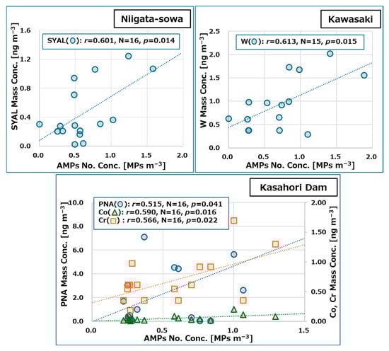
Figure 7.
Scatter plots and linear approximation curves, along with the number of samples (N), the correlation coefficients (r), and the p-values (p) of mass concentrations of PM2.5 components, that exhibited a significant correlation (p < 0.05) with the number concentrations of AMPs, disaggregated by location. The acronyms of each component are presented in Table A4 and the following caption: SYAL: syringaldehyde, W: tungsten, PNA: pinonic acid, Co: cobalt, Cr: chromium.
In Niigata-sowa, a relatively strong correlation between AMPs number concentration and syringaldehyde (SYAL) mass concentration was observed. SYAL is one of the aldehydes yielded by the fragmentation or depolymerization of lignin, which constitutes 20% of the global biomass [83]. SYAL is also recognized as an organic marker of PM2.5 components resulting from biomass combustion [84]. As previously stated in Section 2.1.1, Niigata-sowa is located in an area characterized by extensive rice cultivation, with sporadic occurrences of open burning of residual rice straw following the harvest. Additionally, the mass concentration of SYAL exhibited a robust correlation with that of vanillin (VLN; r = 0.84), which is also an aldehyde derived from lignin. In light of the findings, a correlation between AMPs and the open burning events of biomass containing rice straw was hypothesized. As Kirchsteiger et al. reported, certain types of AMPs—namely, those composed of PE or PP—were suggested to function as carriers for specific PAHs contained in PM2.5 [39]. Despite the fact that this study focused on disparate organic components, there is a possibility that it captured phenomena analogous to those reported in the aforementioned study, specifically working as carriers for PM organic components. However, it should be noted that no significant correlation was found between AMPs and other biomass combustion markers such as levoglucosan (LEV) and mannosan (MAN), nor terephthalic acid (TPA) as a plastic combustion marker (p > 0.05) [85]. Furthermore, it is also important to note that a direct comparison between this study and the aforementioned report is precluded by the difference in sampling durations (approximately 7 days and 24 h, respectively).
In Kawasaki, a relatively strong correlation between AMP number concentration and tungsten (W) mass concentration was observed. W has garnered significant attention for its exceptional performance across a wide range of applications, from household items to cutting-edge research, manufacturing, and military fields. The primary products encompass tungsten carbide, alloys, corrosion-resistant coatings, catalysts, semiconductors, fire-resistant compounds, electrical and electronic products, lighting, and so on [86]. W has minimal natural presence in the atmosphere; however, anthropogenic activities have the potential to cause elevated levels of W [87]. In this study, the mean mass concentration of W in PM2.5 at each location was determined to be 0.94 ± 0.56 ng m−3 in Kawasaki, 0.33 ± 0.24 ng m−3 in Niigata-sowa, and 0.25 ± 0.19 ng m−3 in Kasahori Dam (N = 15 for Kawasaki, N = 16 for the other two sites). A significant discrepancy was identified in the W mass concentration in Kawasaki when compared with the concentrations observed in the other two locations (p < 0.01), while the differences between Niigata-Sowa and Kasahori Dam were not found to be statistically significant (p > 0.05). As previously stated in Section 2.1.1, Kawasaki is the most urban of the three locations, with factories in the port area and small factories engaged in lathe work scattered throughout residential areas. Additionally, the sampling site is situated adjacent to a major thoroughfare, which results in significant vehicular traffic. Consequently, it was considered that the atmospheric concentration levels of W at the three locations were influenced by site attributes, particularly the number and types of anthropogenic sources. In contrast, the nature of the interaction between W and AMPs remains elucidated. As indicated by earlier studies, the presence of heavy metals on the surface of microplastics can be attributable to the plastics’ inherent adsorbent properties, although these behaviors are influenced by various factors [88,89]. However, it is imperative to acknowledge that the aforementioned studies exclusively focused on interactions occurring in aqueous solutions and did not address interactions that may occur in the atmosphere, as well as not focusing on W.
In Kasahori Dam, relatively strong correlations between AMPs number concentration and mass concentrations of cobalt (Co), chromium (Cr), and pinonic acid (PNA) were observed, respectively. Co is a metal that has a variety of applications, including use in pigments, lithium-ion battery electrodes, ceramic paints and glazes, battery manufacturing, and incinerators. It was observed that the mass concentration of this metal in PM2.5 increases significantly in association with anthropogenic sources [90]. Cr is regarded as a constituent of PM2.5, with its primary sources being coal combustion, industry, and transportation (e.g., vehicle tailpipes, brakes, and tire wear), and is believed to be significantly associated with human activities [91]. In this study, a significant discrepancy was identified in both Co and Cr mass concentration in Kawasaki when compared with the concentrations observed in the other two locations (p < 0.01), while the differences between Niigata-Sowa and Kasahori Dam were not found to be statistically significant (p > 0.05), which was consistent with the previous reports mentioned above. In contrast, as discussed in Section 2.1.1, the Kasahori Dam is situated in a region with minimal artificial sources and alternative explanations are imperative when discussing the relationship between Co or Cr mass concentrations and AMP number concentrations. Cr is known to be incorporated into plastics as a coloring pigment [92], and there were a few reports of the presence of heavy metals, including Co and Cr, in MPs found in the aquatic environments [93,94]. Consequently, at the Kasahori Dam, where anthropogenic sources are limited, it was hypothesized that the correlation between heavy metals adsorbed to AMPs, whether intentionally or unintentionally, was comparatively robust in comparison to PM tracer components. PNA is classified as a monoterpene tracer due to its synthesis as a secondary product of α-pinene, which is known as one of the biogenic volatile organic compounds (BVOC), through photochemical oxidation. According to the extant literature, there was an increase in PNA concentrations during the warm season, concurrent with the period of active vegetation [95]. However, in this study, PNA concentrations were lowest in summer, and this trend was also observed at the other two locations (see Table A5), which stood in contrast to the results of the aforementioned report. A previous study demonstrated that PNA exhibited high volatility and predominantly existed in gaseous form at temperatures ranging from 275 to 300 Kelvin [96]. Additionally, it was also reported that gaseous PNA was adsorbed onto quartz fiber filter paper and was barely collected as particles under a 24-h sampling duration [97]. Consequently, it was postulated that the mass concentration variation of PNA in this study was significantly influenced by the artifacts such as gas adsorption, thereby challenging the discussion of its correlation with the number concentration of AMPs.
In light of the aforementioned results and discussion, it was concluded that the utilization of PM tracer components to elucidate the true state of AMPs yielded insights that were instrumental in the estimation of emission sources or analogous information. However, it was also recognized that exploring more effective methods for estimating the source of emissions, including avoiding the influence of artifacts and performing multivariate analysis with an increased number of samples rather than simple regression analysis, was necessary.
3.4. Back-Trajectory Clustering and Its Implication for AMP Transport
As delineated in Figure 8, the plan views of trajectory clusters (Nos. 1 to 4) at each location, as well as their presence ratio throughout the year and on a weekly basis, are presented. As delineated in Section 2.4.2, the optimal number of clusters was determined to be four for each location. Despite the presence of minor variations in trajectory clusters across different locations, a generalizable summary of each trajectory is as follows:

Figure 8.
Plan views of trajectory clusters (Nos. 1 to 4) at each location, as well as their presence ratio throughout the year and on a weekly basis.
- Cluster No. 1: Air masses flowing into Japan from the southeast, circling around the periphery of Pacific high.
- Cluster No. 2: Air masses flowing into Japan from the north to northwest via Primorsky Krai in Russia.
- Cluster No. 3: Air masses flowing into Japan from the northwest via Siberia and northeastern China.
- Cluster No. 4: Air masses, located slightly south of Cluster No.3, flowing into Japan via Siberia, Mongolia, northeastern China, the Korean Peninsula.
It was observed that, across all locations, Cluster No.3 and 4 exhibited a tendency to predominate during the winter season, while Cluster No.2 demonstrated a similar tendency during the spring season. Additionally, both Clusters No.1 and 2 were predominant during the autumn season. In Kawasaki, located on the Pacific coast, the air masses classified as Cluster No.1 accounted for one-third of the total amount, which was particularly significant in summer. Conversely, Niigata-sowa, situated on the Sea of Japan, exhibited a slightly lower frequency of Cluster No.1 compared to Kawasaki, while Clusters No.2 to 4 demonstrated relatively high frequencies. At Kasahori Dam, which is situated on the Sea of Japan side but inland, the cluster distribution was intermediate between that of Niigata-sowa and Kawasaki. In the summer season, the presence of air masses belonging to Cluster No.1 in Niigata-sowa and Kasahori Dam on the Sea of Japan side was infrequent, in contrast to the patterns observed in Kawasaki. Although the aforementioned back trajectory clustering demonstrated some reasonable results, no substantial correlation was identified between the concentration of AMPs and the incidence rate of each cluster at each sampling site (p > 0.05). In Niigata-sowa, a quasi-significant correlation (r = 0.47, p = 0.065) with the occurrence rate of Cluster No. 1 was obtained, and the possibility that AMPs flowed in due to air masses corresponding to the peripheral flow of Pacific high cannot be ruled out. However, given that the aforementioned trend was not observed at the other two locations and that the mass concentration of tracer components that exhibited a significant correlation with the number concentration of AMPs differed at each location as discussed in Section 3.3, it was suggested that local or site-specific factors, rather than transboundary and long-range factors, were predominant in the context of air pollution by AMPs. In general, particles of smaller size demonstrate a greater propensity to travel over greater distances. Therefore, in the context of the future prospects, the contribution rates of local and transboundary air pollution might be predicted through the aerodynamic size-fractionated sampling of AMPs.
4. Conclusions
Airborne microplastics (AMPs) were consistently detected at all three sites, underscoring their ubiquity in diverse atmospheric environments. Polyethylene (PE) was the most abundant polymer, followed by polyethylene terephthalate (PET) and polyamide (PA). Morphologically, fragments predominated across sites, and most particles were smaller than 10 μm, highlighting the predominance of the inhalable fraction. Distinct compositional patterns were observed among the sites. At Niigata-sowa, plastic resins (RES) were more prevalent, while Kawasaki exhibited higher proportions of PET and polyhydroxybutyrate (PHB). At Kasahori Dam, ethylene-vinyl acetate (EVA) was comparatively enriched. These contrasts may reflect the influence of local emission sources and environmental conditions on AMP profiles.
Regression analyses revealed significant correlations between AMP concentrations and selected PM2.5 constituents. At Niigata-sowa, positive associations were found with syringaldehyde (SYAL), a biomass-burning marker. At Kawasaki, correlations emerged with tungsten (W), a traffic- and industry-related metal. At Kasahori Dam, AMPs were linked to cobalt (Co) and chromium (Cr), elements commonly used as plastic additives or possibly present due to non-intentional adsorption. Importantly, the temporal variations of AMPs did not always mirror those of PM mass or chemical species, indicating that AMP dynamics are influenced by additional factors beyond conventional particulate matter processes, and may not be directly inferred from PM behavior alone.
The observed correlations and compositional differences provide new insights into potential AMP sources. Although direct source attribution remains challenging, the findings collectively indicate contributions from traffic, industrial activities, biomass burning, and secondary atmospheric processes. These results underscored the value of integrating AMP measurements with established PM2.5 analyses for source characterization. From a methodological perspective, µRaman spectroscopy proved effective for polymer identification, enabling simultaneous assessment of size and morphology within complex atmospheric matrices. While not a novel technique, its application in conjunction with multi-component PM2.5 analysis in this study demonstrates its continuing relevance and utility for the AMPs research field.
This study is limited by the number of samples, and uncertainties remain in polymer identification, particularly at the submicron scale. Future efforts should extend temporal and spatial monitoring, refine analytical protocols for nanoscale plastics, and further integrate AMP analysis with established source apportionment methods to strengthen environmental and health assessments. Furthermore, future work should implement aerodynamic size-selective sampling to resolve aerodynamic diameter, which is essential for interpreting atmospheric transport processes and assessing potential health implications of airborne microplastics.
Author Contributions
Conceptualization, H.S.; methodology, H.S.; investigation—field research, H.S., T.T., M.F., T.E., M.H. and Y.K.; investigation—analysis, H.S., T.T., M.F. and K.-O.P.; supervision, H.S.; drafting, reviewing, and editing, H.S., T.T., M.F., T.E., M.H. and Y.K. All authors have read and agreed to the published version of the manuscript.
Funding
This work was supported by JSPS KAKENHI Grant Number JP23K11468.
Institutional Review Board Statement
Not applicable.
Informed Consent Statement
Not applicable.
Data Availability Statement
The data presented in this study are available from the first author upon request.
Acknowledgments
The authors would like to express their sincere gratitude to Hiroshi Okochi and the members of his laboratory at Waseda University for their valuable technical advice and guidance throughout this study. The Raman spectrometer was rented from the Technical Management Center, Industrial Research Institute of Niigata Prefecture. The air sample collection space at Kasahori Dam station was made available through the cooperation of the Kasahori Branch Office, Sanjo Regional Development Bureau, Niigata Prefecture.
Conflicts of Interest
The authors declare no conflicts of interest.
Appendix A
Appendix A.1. Supporting Tables
Table A1.
Attributes and detailed characteristics at each sampling site.
Table A1.
Attributes and detailed characteristics at each sampling site.
| Site/Attribute | Characteristics |
|---|---|
| Kawasaki (urban) |
|
| Niigata-sowa (semi-urban) |
|
| Kasahori Dam (rural) |
|
Table A2.
Original names and their acronyms of the target components analyzed in this study.
Table A2.
Original names and their acronyms of the target components analyzed in this study.
| Components | Acronyms | Components | Acronyms | Components | Acronyms |
|---|---|---|---|---|---|
| ions | organics | ||||
| chloride | Cl− | ammonium | NH4+ | malonic acid | MA |
| nitrate | NO3− | potassium | K+ | succinic acid | SCA |
| sulfate | SO42− | magnesium | Mg2+ | glutaric acid | GA |
| sodium | Na+ | calcium | Ca2+ | adipic acid | AA |
| 2,3-dihydroxy-4-oxopentanoic acid | DHOPA | ||||
| inorganic elements | pinonic acid | PNA | |||
| aluminum | Al | selenium | Se | vanillin | VLN |
| titanium | Ti | rubidium | Rb | pimelic acid | PMA |
| vanadium | V | cadmium | Cd | 4-hydroxybenzoic acid | 4-HBA |
| chromium | Cr | antimony | Sb | mannosan | MAN |
| manganese | Mn | cesium | Cs | phthalic acid | PTA |
| iron | Fe | barium | Ba | syringaldehyde | SYAL |
| cobalt | Co | lanthanum | La | suberic acid | SBA |
| nickel | Ni | cerium | Ce | levoglucosan | LEV |
| copper | Cu | samarium | Sm | vanillic acid | VA |
| zinc | Zn | tungsten | W | isophthalic acid | PIA |
| arsenic | As | lead | Pb | terephthalic acid | TPA |
| Azelaic acid | AZA | ||||
| Cholesterol | CHOL | ||||
Table A3.
A summary of the GC/MS analytical conditions.
Table A3.
A summary of the GC/MS analytical conditions.
| Items | Conditions/Settings |
|---|---|
| GC | |
| Capillary column | InertCap 5MS/Sil (30 m, 0.25 mm I.D., 0.25 µm f.t.) |
| Injection mode | Splitless |
| Injection volume | 1 µL |
| Injection temperature | 270 °C |
| Oven temperature | 80 °C (3 min)-3 °C/min-200 °C (2 min)-15 °C/min-300 °C (15 min) |
| Carrier gas | He(1 mL/min) |
| MS | |
| Interface temperature | 270 °C |
| Ion source temperature | 230 °C |
| Ionization | EI |
| Detection mode | SIM |
Table A4.
Original names and their acronyms for AMP polymer types identified in this study.
Table A4.
Original names and their acronyms for AMP polymer types identified in this study.
| Acronyms | Polymer Names |
|---|---|
| PE | Polyethylene |
| PET | Polyethylene terephthalate |
| PA | Polyamide |
| PS | Polystyrene |
| PHB | Polyhydroxybutyrate |
| RES | Plastic resin (i.e., Epoxy resin, Phenoxy resin) |
| EVA | Ethylene-vinyl acetate |
| PVA | Polyvinyl alcohol |
| PP | Polypropylene |
| PUR | Polyurethane |
| PEster | Polyester (excluding PET) |
| PE/PP | Copolymer of Polyethylene/Polypropylene |
| PPS | Polyphenylene sulfide |
| PS/PVC | Copolymer of Polystyrene/Polyvinyl chloride |
| PMMA | Polymethyl methacrylate |
| PVC | Polyvinyl chloride |
Table A5.
Annual average values of pinonic acid (PNA) mass concentrations in PM2.5 at each site.
Table A5.
Annual average values of pinonic acid (PNA) mass concentrations in PM2.5 at each site.
| Site/Attribute | Winter (2023) | Spring (2024) | Summer (2024) | Autum (2024) |
|---|---|---|---|---|
| Kasahori Dam/rural | 3.96 ± 2.38 | 5.97 ± 3.33 | 0.02 ± 0.00 | 0.55 ± 0.31 |
| Niigata-sowa/semi-urban | 2.83 ± 1.72 | 2.29 ± 0.57 | 0.02 ± 0.00 | 0.77 ± 0.65 |
| Kawasaki/urban | 3.46 ± 4.19 | 3.44 ± 3.18 | 0.02 ± 0.00 | 0.62 ± 0.14 |
Note: unit: ng m−3.
Appendix A.2. Supporting Figures

Figure A1.
Satellite images which delineate Niigata-sowa and Kawasaki as well as the nearest meteorological station (AMeDAS) to each of the sampling sites.

Figure A2.
Variations of total spatial variance (TSV) with cluster numbers at each receptor site during the clustering of back trajectories.

Figure A3.
Weekly fluctuations of AMPs number concentrations (conc.) as TSP, ion mass conc. of PM2.5/PMc, and the predominant wind directions at each sampling site. * If “calm (wind speed < 0.3 m/s)” is the most frequent, it will display as “C.”.

Figure A4.
Raman spectra of polyhydroxybutyrate (PHB) from the KnowItAll library (orange, top row) and the identified AMP (black, bottom row), along with an actual field-of-view image of the AMP.

Figure A5.
Breakdowns of AMP morphologies (fragment, granule and fiber) for the total and individual sampling sites. The distinction among morphologies was made according to the definition of aspect ratio shown in Section 2.2.2.
Appendix B
Appendix B.1. Supporting Notes
Note that the references in this section correspond to those listed in the main article.
Appendix B.1.1. Sampling Methods
AMPs and PM were measured in parallel using different filter papers and their holders simultaneously at the three sites. AMPs were collected as total suspended particles (TSP) on a PTFE filter paper (ADVANTEC, T080A047A, pore size: 0.8 μm) using a single stage holder (SIBATA, TF-4) made of PTFE or fluoro rubber. Conversely, PM was collected using a polycarbonate two-stage holder (NILU, NL-O-02) and a PM2.5 cascade impactor (Tokyo Dylec, NL-10-2.5P) on quartz fiber filter papers (PALL, 2500QAT-UP) of different shapes to separate PM2.5 and particles larger than 2.5 μm in diameter (hereinafter referred to as “PMc”). During the collection process, each filter paper holder was placed within a metal windshield, and the air was continuously aspirated for a period of 6–8 days at a flow rate of 10 L/min (converted to 20 °C). For PM, a low-volume air pump with flow control function (SIBATA, LVS-30) was utilized to achieve classified collection, and for AMPs, a combination of a low-volume air pump (ULVAC, DA-60S, etc.) and a mass flow meter (Azbil, CMS0050BSRN200000) was employed. The total air suction amount per sample was set at a minimum of 70 m3, given the documented susceptibility to AMPs contamination. An intensive sample collection period of approximately one month was established for each season, and four samples were obtained per period, for a total of 16 samples per sample collection site. Periods and days for sample collection of each sample per season were shown in the following Table A6.
Table A6.
Periods and days for sample collection of each sample per season.
Table A6.
Periods and days for sample collection of each sample per season.
| Spl. No. | Winter (2023) | Spring (2024) | Summer (2024) | Autumn (2024) | ||||
|---|---|---|---|---|---|---|---|---|
| Period | Days | Period | Days | Period | Days | Period | Days | |
| No.1 | 14 NOV−21 NOV | 7 | 26 MAR−2 APR | 7 | 8 JUL−16 JUL | 8 | 9 SEP−17 SEP | 8 |
| No.2 | 21 NOV−28 NOV | 7 | 2 APR−10 APR | 8 | 16 JUL−23 JUL | 7 | 17 SEP−24 SEP | 7 |
| No.3 | 28 NOV−5 DEC | 7 | 10 APR−16 APR | 6 | 23 JUL−30 JUL | 7 | 24 SEP−30 SEP | 6 |
| No.4 | 5 DEC−12 DEC | 7 | 16 APR−23 APR | 7 | 30 JUL−6 AUG | 7 | 30 SEP−7 OCT | 7 |
In accordance with the provisions stipulated in the EANET technical manual [40], in instances where data completeness dipped below the 70% threshold due to circumstances such as power outages or equipment malfunctions, the data were subsequently excluded from further analysis.
Appendix B.1.2. Preparation for AMPs Samples
The following procedures were performed in a clean room (AIRTECH, APB558S) wearing a 100% cotton lab coat and nitrile gloves (KIMTECH, Vista) and the reagents were filtered prior to use through hydrophilic PTFE filter papers (ADVANTEC, H050A047A, pore size: 0.5 μm) to mitigate the risk of plastic contamination. In the context of extant studies, sample preparation can be broadly categorized into three distinct processes: (i) organic matter decomposition, (ii) heavy liquid (gravity) separation, and (iii) centrifugation. Figure A2 illustrates a flow diagram delineating the outline protocol for preparation of AMPs samples.
The PTFE filter paper collected in Section 2.1.2 was extracted with 20 mL of ultrapure water in a glass centrifuge tube (SANSYO, 84-1304) using a shaker (TAITEC, SR-1D) for 120 min at 130 rpm. The solution in the centrifuge tube and the glassware that had been in contact with the solution were meticulously washed 4 to 5 times with ultrapure water and filtered under reduced pressure through a hydrophilic PTFE filter paper (ADVANTEC, H050A025A, pore size: 0.5 μm). The filter paper was placed in the same centrifuge tube with 20 mL of 30.0–35.5% hydrogen peroxide (H2O2, Kanto Chem., 18084-00), heated and stirred at 60 °C for 24 h, and then filtered again through a new hydrophilic PTFE filter paper. The centrifuge tube and glassware were meticulously washed four to five times with ultrapure water and the solution was filtered. The filter paper was placed in the same centrifuge tube with 30 mL of sodium iodide (NaI) solution, which had been prepared from powder NaI reagent (Junsei Chem., 80240-1201) and ultrapure water to a specific gravity (ρ) of 1.5. The tube was shaken with the same shaker for 120 min at 150 rpm and then centrifuged for 60 min at 2,500 rpm using a HITACHI himac CT6D centrifuge. After standing for a minimum of 60 min, the upper 15 mL of the solution was taken and filtered through alumina filter paper (Cytiva, Whatman® Anodisc® 25, pore size: 0.2 μm). The centrifuge tube and glassware were meticulously washed four to five times with ultrapure water, after which the solution was filtered. The alumina filter paper was transferred to a glass petri dish and thoroughly dried in an auto dry desiccator (AS ONE, OH-3S) with a low relative humidity (<30%) at room temperature. The sample that underwent this preparation method was used for the identification of AMPs as described in Section 2.2.2.
The preparation process resulted in concentration of the effective filtration area of the sample from φ40 mm to φ4 mm. Furthermore, this process eliminates organic and inorganic materials that are not plastics, as well as biofilm on the plastic surface, which will enhance the accuracy of subsequent Raman microscopy measurements [13,17].
Appendix B.1.3. Identification of AMPs
Raman spectra were measured using a laser Raman spectroscopy (JASCO, NRS-4500; hereafter referred to as “μRaman”) under the measurement conditions and settings delineated in Table 1. The superiority of μRaman in terms of spatial resolution and sensitivity, particularly in detecting AMPs with a diameter of less than 20 μm [48], establishes it as the preeminent spectroscopic method for AMPs with a diameter of less than 2.5 μm [38].
However, two major concerns in μRaman measurements should be noted: damage to the sample caused by laser irradiation and spectral interference due to fluorescence [17,38,49,50]. As part of the countermeasure for sample damage in this study, the following initial conditions were determined: laser output of 1%, accumulation count of 3 times, and exposure time of 5 s. After confirming that the acquisition of measurements could be conducted the initial conditions without any impediments, the measurement conditions were adjusted and optimized below the upper limits established at a laser output of 5%, an accumulation count of 5 times, and an exposure time of 10 s. Under this measurement protocol, any damage accompanied with changes in the Raman spectrum were not observed among all the samples measured. Also, to address the issue of fluorescent interference, a variety of sizes of pinhole-shaped spectroscope slits were employed, including φ100 μm, φ34 μm, φ17 μm, in lieu of rectangular-shaped ones. The three slits were able to be switched immediately, and the most preferable one was selected for measurement in each sample by checking the observation spectra. Nevertheless, it is challenging to entirely eliminate the influence of fluorescence due to the characteristics of μRaman and the influence of colorants used in plastics [51], and this point must be noted while interpreting the results.
The alumina filter obtained in Section 2.2.1 was set in the μRaman, and all particles and fibers observed in the actual field of view image of the 100× objective lens (field of view: 140 μm × 110 μm) were targeted for the following screening: The laser for observation (power output: 0.0001%) was irradiated onto the particles and fibers, and the presence or absence of peaks appearing around 2800–3000 cm−1, which correspond to C-H stretching vibration, was confirmed from the observation spectra obtained. After the screening, the actual measurements were performed exclusively on particles and fibers that exhibited C-H stretching vibrations, in accordance with the conditions delineated in Table 1 and the protocol described in the previous paragraph. The obtained Raman spectra were then compared with the spectra library (Wiley, KnowItAll), and when the “Hit Quality Index (HQI)” was 75 or higher and plastics were identified as the top match, the particles and fibers were identified as plastics. The HQI is a metric of spectral consistency, with 100 representing a perfect match and 0 representing a complete mismatch. The analysis tool integrated within μRaman was utilized to obtain actual images and to measure the particle sizes (i.e., Feret and short diameters). The shapes of AMPs were determined based on WHO guidelines and previous studies [53,54]. In this study, fibers were defined as those with an aspect ratio of Feret diameter to short diameter greater than 3:1; Particles were defined as those with an aspect ratio less than 1.2:1; Fragments were defined as those with an aspect ratio between the two categories.
The aforementioned operation was replicated on 30 occasions (i.e., fields of view), with the number of AMPs being enumerated for each sample. To ensure the absence of overlap of each field of view, the coordinate memory function of μRaman was utilized in 30 occasions. The effective filtration area of φ4 mm was separated into two concentric circles: the central and fringe strata. Measurements were taken evenly 15 times in each stratum. The number concentration of AMPs was calculated using the equation (1) delineated in Section 2.2.2. Although the spatial resolution of the μRaman utilized in this study is not specified by the manufacturer, it is generally accepted to be approximately 1 μm for models with standard specifications [38], with the exception of high-end configurations [50,52]. Given that the pore size of the filter paper utilized for AMPs collection was 0.8 μm and the minimum Feret diameter of the identified AMPs exceeded 1 μm, this study focused on AMPs larger than 1 μm in Feret diameter. All reported particle sizes represent geometric diameters derived from image analysis and are not directly equivalent to aerodynamic diameters, particularly for irregular, low-density plastic particles. Because the measurement was based solely on the optical projection of TSP-collected particles, conversion to aerodynamic diameter is not possible from the current dataset without additional information on particle density, shape, and dynamic shape factors.
In addition, as part of QA/QC for AMPs samples, the PTFE filter papers, which were identical to ones for the actual samples, were prepared for the operational blanks (N = 3) and travel blanks (N = 1 at each sampling site). The same sample preparation and identification methods described in Section 2.2 were employed. Consequently, no AMPs were identified in any of the blanks, thereby confirming that the impact of contamination using the methods employed in this study was minimal. Plus, this study determined a successful qualitative recovery according to the protocol reported in the previous study, which demonstrated a spike-and-recovery test using φ10 μm polystyrene beads [17]. This was done to determine whether the preparation process has a risk of AMP loss.
Appendix B.1.4. PM Sample Preparation and Analysis
The quartz fiber filter papers collected in Section 2.1.2 were meticulously divided into quarter-sized pieces on the collection surface using an acrylic knife, and each quarter was subjected to analysis for ion and inorganic element components in both PM2.5 and PMc, and organic components in PM2.5 only. The manuals published by the Ministry of the Environment, Japan and previous studies were used as references for the sample preparation of each PM component [45,55,56,57,58]. As delineated in Table A2, the original names and their acronyms for of the target components analyzed in this study are enumerated.
The following operations were performed in preparation for ion components: The quarter-sized filter paper was placed in a plastic centrifuge tube (AS ONE, C571-2) with 15 mL of ultrapure water and extracted with shaking for 20 min at 110 rpm using a shaker (TAITEC, SR-1D). The extract was filtered through a syringe filter (ADVANTEC, DISMIC 25HP045AN, pore size: 0.45 μm) and the resulting filtrate was subjected to measurement in an ion chromatograph (Thermo Fisher Scientific, DIONEX Integrion HPIC) to determine the concentration of 8 ions delineated in Table A2. The plastic container for the filtrate was refrigerated until the analysis was to be conducted, and measurements were, in principle, performed by the day after the date of extraction to avoid alterations in composition after extraction.
The following operations were performed in preparation for inorganic element components: The quarter-sized filter paper, 6 mL of nitric acid (HNO3: Kanto Chem., EL (1.38), 28163-09), 3 mL of hydrofluoric acid (HF: Tama Chem., TAMAPURE-AA-100), and 1 mL of H2O2 (Kanto Chem., UltrapurTM, 18084-2B) are to be placed in a dedicated fluororesin vessel and completely sealed. The filter paper was decomposed in a microwave for acid decomposition (Milestone General, ETHOS EASY) until complete dissolution was achieved. Using the same microwave, the solution was concentrated until it was one drop in size, at which point it was transferred to a metal-free centrifuge tube (Labcon, 3134-345MP). The volume of the centrifuge tube was increased by 2% (v/v) HNO3, which had been prepared using the HNO3 reagent and ultrapure water. Following a thorough cleansing of the fluororesin vessel with a total of four to five washings, the solution was subsequently introduced into the same tube precisely up to 10 mL. The centrifuge tube was refrigerated until the measurement. As an internal standard, 2.5 mL of indium solution (10 ng mL−1) was added, which had been previously prepared with indium standard solution (Kanto Chem., 20241-1B) and aforementioned 2% (v/v) HNO3, and used for ICP-MS measurement (Thermo Fisher Scientific, iCAP Qc) to determine the concentration of 22 inorganic elements delineated in Table A2.
The following operations were performed in preparation for organic components: A quarter of a quartz fiber filter was placed into a 5 mL glass test tube, to which 1 µg each of ketopinic acid (Wako Pure Chem., 325-50551) and Levoglucosan-13C6 (Cambridge Isotope Laboratories, Inc., CLM-4748-1.2) were added as internal standards. Subsequently, 5 mL of a 2:1 (v/v) dichloromethane/methanol mixture (Kanto Chem., 10158-3B/25183-4B) was added, and ultrasonic extraction was performed for 15 min using an ultrasonic cleaner (Bransonic, CPX5800H-J). The resulting solution was filtered through a PTFE filter (ADVANTEC, DISMIC 25HP045AN, pore size: 0.45 µm) using a glass syringe, and the filtrate was collected. The extract was then evaporated to dryness under a gentle nitrogen stream at 50 °C using a dry block heater (EYELA, MG-3100). The residue was reconstituted with 150 µL of a 1:1 (v/v) dichloromethane/hexane mixture (Kanto Chem., 10158-3B/18041-3B), and 50 µL of N,O-bis(trimethylsilyl)trifluoroacetamide containing 10% chlorotrimethylsilane (Wako Pure Chem., 021-17703) was added. The solution was tightly sealed and heated at 70 °C for 2 h using the same dry block heater to derivatize the analytes into their trimethylsilyl derivatives. The resulting derivatized sample was then subjected to GC/MS analysis (Shimadzu, GCMS-QP2020 NX) without delay to determine the concentration of 19 organics delineated in Table A2. If immediate analysis was not possible, the sample was frozen and measured within one week. The GC/MS analytical conditions were summarized in Table A3.
As part of QA/QC for PM samples, the quartz fiber filter papers, which were identical to ones for the actual samples, were prepared for the operational blanks (N = 3) per season. The same sample preparation and measurement methods described in 2.3 were employed for all components. The median of the 3 blank values were subtracted from the sample values before calculation of atmospheric concentrations. For all components, the detection limits were defined as three times the standard deviation of either the blank values or the repeated lowest standard solutions for the calibration curves. In instances where the measured values fell below the detection limits, they were treated as half of the detection limits.
References
- World Economic Forum. The New Plastics Economy: Rethinking the Future of Plastics. Available online: https://jp.weforum.org/publications/the-new-plastics-economy-rethinking-the-future-of-plastics/ (accessed on 9 May 2025).
- Hartmann, N.B.; Hüffer, T.; Thompson, R.C.; Hassellöv, M.; Verschoor, A.; Daugaard, A.E.; Rist, S.; Karlsson, T.; Brennholt, N.; Cole, M.; et al. Are We Speaking the Same Language? Recommendations for a Definition and Categorization Framework for Plastic Debris. Environ. Sci. Technol. 2019, 53, 1039–1047. [Google Scholar] [CrossRef] [PubMed]
- Eriksen, M.; Lebreton, L.C.M.; Carson, H.S.; Thiel, M.; Moore, C.J.; Borerro, J.C.; Galgani, F.; Ryan, P.G.; Reisser, J. Plastic Pollution in the World’s Oceans: More than 5 Trillion Plastic Pieces Weighing over 250,000 Tons Afloat at Sea. PLoS ONE 2014, 9, e111913. [Google Scholar] [CrossRef] [PubMed]
- Zhao, S.; Kvale, K.F.; Zhu, L.; Zettler, E.R.; Egger, M.; Mincer, T.J.; Amaral-Zettler, L.A.; Lebreton, L.; Niemann, H.; Nakajima, R.; et al. The Distribution of Subsurface Microplastics in the Ocean. Nature 2025, 641, 51–61. [Google Scholar] [CrossRef] [PubMed]
- Kameda, Y.; Yamada, N.; Fujita, E. Source- and Polymer-Specific Size Distributions of Fine Microplastics in Surface Water in an Urban River. Environ. Pollut. 2021, 284, 117516. [Google Scholar] [CrossRef]
- Nihei, Y.; Yoshida, T.; Kataoka, T.; Ogata, R. High-Resolution Mapping of Japanese Microplastic and Macroplastic Emissions from the Land into the Sea. Water 2020, 12, 951. [Google Scholar] [CrossRef]
- Free, C.M.; Jensen, O.P.; Mason, S.A.; Eriksen, M.; Williamson, N.J.; Boldgiv, B. High-Levels of Microplastic Pollution in a Large, Remote, Mountain Lake. Mar. Pollut. Bull. 2014, 85, 156–163. [Google Scholar] [CrossRef]
- Scheurer, M.; Bigalke, M. Microplastics in Swiss Floodplain Soils. Environ. Sci. Technol. 2018, 52, 3591–3598. [Google Scholar] [CrossRef]
- Zhou, Y.; Wang, J.; Zou, M.; Yin, Q.; Qiu, Y.; Li, C.; Ye, B.; Guo, T.; Jia, Z.; Li, Y.; et al. Microplastics in Urban Soils of Nanjing in Eastern China: Occurrence, Relationships, and Sources. Chemosphere 2022, 303, 134999. [Google Scholar] [CrossRef]
- Sunaga, N.; Okochi, H.; Niida, Y.; Miyazaki, A. Alkaline Extraction Yields a Higher Number of Microplastics in Forest Canopy Leaves: Implication for Microplastic Storage. Environ. Chem. Lett. 2024, 22, 1599–1606. [Google Scholar] [CrossRef]
- Tokunaga, Y.; Okochi, H.; Tani, Y.; Niida, Y.; Tachibana, T.; Saigawa, K.; Katayama, K.; Moriguchi, S.; Kato, T.; Hayama, S. Airborne Microplastics Detected in the Lungs of Wild Birds in Japan. Chemosphere 2023, 321, 138032. [Google Scholar] [CrossRef]
- Dris, R.; Gasperi, J.; Mirande, C.; Mandin, C.; Guerrouache, M.; Langlois, V.; Tassin, B. A First Overview of Textile Fibers, Including Microplastics, in Indoor and Outdoor Environments. Environ. Pollut. 2017, 221, 453–458. [Google Scholar] [CrossRef] [PubMed]
- Allen, S.; Allen, D.; Phoenix, V.R.; Le Roux, G.; Durántez Jiménez, P.; Simonneau, A.; Binet, S.; Galop, D. Atmospheric Transport and Deposition of Microplastics in a Remote Mountain Catchment. Nat. Geosci. 2019, 12, 339–344. [Google Scholar] [CrossRef]
- Allen, S.; Allen, D.; Moss, K.; Le Roux, G.; Phoenix, V.R.; Sonke, J.E. Examination of the Ocean as a Source for Atmospheric Microplastics. PLoS ONE 2020, 15, e0232746. [Google Scholar] [CrossRef] [PubMed]
- Allen, S.; Allen, D.; Baladima, F.; Phoenix, V.R.; Thomas, J.L.; Le Roux, G.; Sonke, J.E. Evidence of Free Tropospheric and Long-Range Transport of Microplastic at Pic Du Midi Observatory. Nat. Commun. 2021, 12, 7242. [Google Scholar] [CrossRef]
- Wang, Y.; Okochi, H.; Tani, Y.; Hayami, H.; Minami, Y.; Katsumi, N.; Takeuchi, M.; Sorimachi, A.; Fujii, Y.; Kajino, M.; et al. Airborne Hydrophilic Microplastics in Cloud Water at High Altitudes and Their Role in Cloud Formation. Environ. Chem. Lett. 2023, 21, 3055–3062. [Google Scholar] [CrossRef]
- Sasaki, H.; Takahashi, T.; Futami, M.; Endo, T.; Hirano, M.; Kotake, Y. A Trial Survey on Atmospheric/Airborne Microplastics Using Micro-Raman Spectroscopy (μRaman). J. Environ. Chem. 2024, 34, 61–70. (In Japanese) [Google Scholar] [CrossRef]
- Amato-Lourenço, L.F.; Carvalho-Oliveira, R.; Júnior, G.R.; Dos Santos Galvão, L.; Ando, R.A.; Mauad, T. Presence of Airborne Microplastics in Human Lung Tissue. J. Hazard. Mater. 2021, 416, 126124. [Google Scholar] [CrossRef]
- Jenner, L.C.; Rotchell, J.M.; Bennett, R.T.; Cowen, M.; Tentzeris, V.; Sadofsky, L.R. Detection of Microplastics in Human Lung Tissue Using μFTIR Spectroscopy. Sci. Total Environ. 2022, 831, 154907. [Google Scholar] [CrossRef]
- Ragusa, A.; Notarstefano, V.; Svelato, A.; Belloni, A.; Gioacchini, G.; Blondeel, C.; Zucchelli, E.; De Luca, C.; D’Avino, S.; Gulotta, A.; et al. Raman Microspectroscopy Detection and Characterisation of Microplastics in Human Breastmilk. Polymers 2022, 14, 2700. [Google Scholar] [CrossRef]
- Ragusa, A.; Svelato, A.; Santacroce, C.; Catalano, P.; Notarstefano, V.; Carnevali, O.; Papa, F.; Rongioletti, M.C.A.; Baiocco, F.; Draghi, S.; et al. Plasticenta: First Evidence of Microplastics in Human Placenta. Environ. Int. 2021, 146, 106274. [Google Scholar] [CrossRef]
- Leonard, S.V.L.; Liddle, C.R.; Atherall, C.A.; Chapman, E.; Watkins, M.; Calaminus, S.D.J.; Rotchell, J.M. Microplastics in Human Blood: Polymer Types, Concentrations and Characterisation Using μFTIR. Environ. Int. 2024, 188, 108751. [Google Scholar] [CrossRef] [PubMed]
- Vethaak, A.D.; Legler, J. Microplastics and Human Health. Science 2021, 371, 672–674. [Google Scholar] [CrossRef] [PubMed]
- Dris, R.; Gasperi, J.; Saad, M.; Mirande, C.; Tassin, B. Synthetic Fibers in Atmospheric Fallout: A Source of Microplastics in the Environment? Mar. Pollut. Bull. 2016, 104, 290–293. [Google Scholar] [CrossRef] [PubMed]
- Liu, C.; Li, J.; Zhang, Y.; Wang, L.; Deng, J.; Gao, Y.; Yu, L.; Zhang, J.; Sun, H. Widespread Distribution of PET and PC Microplastics in Dust in Urban China and Their Estimated Human Exposure. Environ. Int. 2019, 128, 116–124. [Google Scholar] [CrossRef]
- Syafei, A.D.; Nurasrin, N.R.; Assomadi, A.F.; Boedisantoso, R. Microplastic Pollution in the Ambient Air of Surabaya, Indonesia. Curr. World Environ. 2019, 14, 290–298. [Google Scholar] [CrossRef]
- Wright, S.L.; Ulke, J.; Font, A.; Chan, K.L.A.; Kelly, F.J. Atmospheric Microplastic Deposition in an Urban Environment and an Evaluation of Transport. Environ. Int. 2020, 136, 105411. [Google Scholar] [CrossRef]
- Abbasi, S.; Keshavarzi, B.; Moore, F.; Turner, A.; Kelly, F.J.; Dominguez, A.O.; Jaafarzadeh, N. Distribution and Potential Health Impacts of Microplastics and Microrubbers in Air and Street Dusts from Asaluyeh County, Iran. Environ. Pollut. 2019, 244, 153–164. [Google Scholar] [CrossRef]
- Aves, A.; Ruffell, H.; Evangeliou, N.; Gaw, S.; Revell, L.E. Modelled Sources of Airborne Microplastics Collected at a Remote Southern Hemisphere Site. Atmos. Environ. 2024, 325, 120437. [Google Scholar] [CrossRef]
- Sridharan, S.; Kumar, M.; Singh, L.; Bolan, N.S.; Saha, M. Microplastics as an Emerging Source of Particulate Air Pollution: A Critical Review. J. Hazard. Mater. 2021, 418, 126245. [Google Scholar] [CrossRef]
- Chen, G.; Feng, Q.; Wang, J. Mini-Review of Microplastics in the Atmosphere and Their Risks to Humans. Sci. Total Environ. 2020, 703, 135504. [Google Scholar] [CrossRef]
- WHO Global Air Quality Guidelines: Particulate Matter (PM2.5 and PM10), Ozone, Nitrogen Dioxide, Sulfur Dioxide and Carbon Monoxide, 1st ed.; World Health Organization: Geneva, Switzerland, 2021; ISBN 978-92-4-003422-8.
- Revell, L.E.; Kuma, P.; Le Ru, E.C.; Somerville, W.R.C.; Gaw, S. Direct Radiative Effects of Airborne Microplastics. Nature 2021, 598, 462–467. [Google Scholar] [CrossRef] [PubMed]
- Kabir, M.S.; Wang, H.; Luster-Teasley, S.; Zhang, L.; Zhao, R. Microplastics in Landfill Leachate: Sources, Detection, Occurrence, and Removal. Environ. Sci. Ecotechnol. 2023, 16, 100256. [Google Scholar] [CrossRef] [PubMed]
- Katsumi, N.; Kusube, T.; Nagao, S.; Okochi, H. Spatiotemporal Variation in Microplastics Derived from Polymer-Coated Fertilizer in an Agricultural Small River in Ishikawa Prefecture, Japan. Environ. Pollut. 2023, 325, 121422. [Google Scholar] [CrossRef] [PubMed]
- Suzuki, G.; Uchida, N.; Tanaka, K.; Higashi, O.; Takahashi, Y.; Kuramochi, H.; Yamaguchi, N.; Osako, M. Global Discharge of Microplastics from Mechanical Recycling of Plastic Waste. Environ. Pollut. 2024, 348, 123855. [Google Scholar] [CrossRef]
- Brahney, J.; Mahowald, N.; Prank, M.; Cornwell, G.; Klimont, Z.; Matsui, H.; Prather, K.A. Constraining the Atmospheric Limb of the Plastic Cycle. Proc. Natl. Acad. Sci. USA 2021, 118, e2020719118. [Google Scholar] [CrossRef]
- Akhbarizadeh, R.; Dobaradaran, S.; Amouei Torkmahalleh, M.; Saeedi, R.; Aibaghi, R.; Faraji Ghasemi, F. Suspended Fine Particulate Matter (PM2.5), Microplastics (MPs), and Polycyclic Aromatic Hydrocarbons (PAHs) in Air: Their Possible Relationships and Health Implications. Environ. Res. 2021, 192, 110339. [Google Scholar] [CrossRef]
- Kirchsteiger, B.; Materić, D.; Happenhofer, F.; Holzinger, R.; Kasper-Giebl, A. Fine Micro- and Nanoplastics Particles (PM2.5) in Urban Air and Their Relation to Polycyclic Aromatic Hydrocarbons. Atmos. Environ. 2023, 301, 119670. [Google Scholar] [CrossRef]
- Network Center for EANET. Technical Manual for Air Concentration Monitoring in East Asia. Available online: https://www.eanet.asia/wp-content/uploads/2019/04/techacm.pdf (accessed on 21 May 2025).
- Mason, R.P. Trace Metals in Aquatic Systems; John Wiley & Sons: Hoboken, NJ, USA, 2013; ISBN 978-1-118-27457-6. [Google Scholar]
- Warneck, P. Chemistry of the Natural Atmosphere, 2nd ed.; This is Volume 71 in the International Geophysics Series; Academic Press: San Diego, CA, USA, 2000; ISBN 978-0-12-735632-7. [Google Scholar]
- Chow, W.S.; Liao, K.; Huang, X.H.H.; Leung, K.F.; Lau, A.K.H.; Yu, J.Z. Measurement Report: The 10-Year Trend of PM2.5 Major Components and Source Tracers from 2008 to 2017 in an Urban Site of Hong Kong, China. Atmos. Chem. Phys. 2022, 22, 11557–11577. [Google Scholar] [CrossRef]
- Fakhri, N.; Fadel, M.; Pikridas, M.; Sciare, J.; Hayes, P.L.; Afif, C. Source Apportionment of PM2.5 Using Organic/Inorganic Markers and Emission Inventory Evaluation in the East Mediterranean-Middle East City of Beirut. Environ. Res. 2023, 223, 115446. [Google Scholar] [CrossRef]
- Tian, Y.; Wang, X.; Zhao, P.; Shi, Z.; Harrison, R.M. PM2.5 Source Apportionment Using Organic Marker-Based Chemical Mass Balance Modeling: Influence of Inorganic Markers and Sensitivity to Source Profiles. Atmos. Environ. 2023, 294, 119477. [Google Scholar] [CrossRef]
- Liu, K.; Wang, X.; Wei, N.; Song, Z.; Li, D. Accurate Quantification and Transport Estimation of Suspended Atmospheric Microplastics in Megacities: Implications for Human Health. Environ. Int. 2019, 132, 105127. [Google Scholar] [CrossRef] [PubMed]
- Hurley, R.R.; Lusher, A.L.; Olsen, M.; Nizzetto, L. Validation of a Method for Extracting Microplastics from Complex, Organic-Rich, Environmental Matrices. Environ. Sci. Technol. 2018, 52, 7409–7417. [Google Scholar] [CrossRef] [PubMed]
- Käppler, A.; Windrich, F.; Löder, M.G.J.; Malanin, M.; Fischer, D.; Labrenz, M.; Eichhorn, K.-J.; Voit, B. Identification of Microplastics by FTIR and Raman Microscopy: A Novel Silicon Filter Substrate Opens the Important Spectral Range below 1300 cm−1 for FTIR Transmission Measurements. Anal. Bioanal. Chem. 2015, 407, 6791–6801. [Google Scholar] [CrossRef] [PubMed]
- Araujo, C.F.; Nolasco, M.M.; Ribeiro, A.M.P.; Ribeiro-Claro, P.J.A. Identification of Microplastics Using Raman Spectroscopy: Latest Developments and Future Prospects. Water Res. 2018, 142, 426–440. [Google Scholar] [CrossRef] [PubMed]
- Harusato, A.; Kato, M. Mechanisms of Generation and Ecological Impacts of Nano- and Microplastics from Artificial Turf Systems in Sports Facilities. Environments 2025, 12, 109. [Google Scholar] [CrossRef]
- Azari, A.; Ronsmans, S.; Vanoirbeek, J.A.J.; Hoet, P.H.M.; Ghosh, M. Challenges in Raman Spectroscopy of (Micro)Plastics: The Interfering Role of Colourants. Environ. Pollut. 2024, 363, 125250. [Google Scholar] [CrossRef]
- Dąbrowska, A.; Mielańczuk, M.; Syczewski, M. The Raman Spectroscopy and SEM/EDS Investigation of the Primary Sources of Microplastics from Cosmetics Available in Poland. Chemosphere 2022, 308, 136407. [Google Scholar] [CrossRef]
- World Health Organization. Determination of Airborne Fibre Number Concentrations: A Recommended Method, by Phase-Contrast Optical Microscopy (Membrane Filter Method); World Health Organization: Geneva, Switzerland, 1997; ISBN 978-92-4-154496-2. [Google Scholar]
- Li, Y.; Shao, L.; Wang, W.; Zhang, M.; Feng, X.; Li, W.; Zhang, D. Airborne Fiber Particles: Types, Size and Concentration Observed in Beijing. Sci. Total Environ. 2020, 705, 135967. [Google Scholar] [CrossRef]
- Ministry of the Environment, Japan. A Manual for the Measurement of Atmospheric Fine Particulate Matter (PM2.5) Components. Available online: https://www.env.go.jp/air/osen/pm/ca/manual.html (accessed on 27 May 2025). (In Japanese)
- Takahashi, T.; Take, N.; Ohizumi, T.; Morohashi, M.; Takahashi, M.; Sase, H. Source Estimation of PM2.5 Observed from 2016 to 2017 in Niigata City Using Organic Marker Components. J. Jpn. Soc. Atmos. Env. 2020, 55, 60–77. (In Japanese) [Google Scholar] [CrossRef]
- Taniguchi, Y.; Shimada, K.; Takami, A.; Lin, N.-H.; Chan, C.K.; Kim, Y.P.; Hatakeyama, S. Transboundary and Local Air Pollutants in Western Japan Distinguished on the Basis of Ratios of Metallic Elements in Size-Segregated Aerosols. Aerosol Air Qual. Res. 2017, 17, 3141–3150. [Google Scholar] [CrossRef]
- Sasaki, H.; Endo, T.; Sato, S.; Take, N.; Mitobe, H.; Yagoh, H. Evaluation of PM2.5 Impactor-Fitted Filter-Pack Method for Dry Deposition Monitoring. J. Jpn. Soc. Atmos. Environ. 2022, 57, 66–76. (In Japanese) [Google Scholar] [CrossRef]
- Japan Meteorological Agency. Downloads: The Past Meteorological Data. Available online: https://www.data.jma.go.jp/risk/obsdl/index.php (accessed on 10 June 2025). (In Japanese)
- National Institute for Environmental Studies, Japan. Global Environmental Database, Trajectory (METEX). Available online: https://db.cger.nies.go.jp/ged/metex/en/index.html (accessed on 13 May 2025).
- Saha, S.; Moorthi, S.; Wu, X.; Wang, J.; Nadiga, S.; Tripp, P.; Behringer, D.; Hou, Y.-T.; Chuang, H.; Iredell, M.; et al. NCEP Climate Forecast System Version 2 (CFSv2) 6-Hourly Products 2011; National Science Foundation: Ann Arbor, MI, USA; National Center for Atmospheric Research (NCAR): Boulder, CO, USA, 2011.
- Sirois, A.; Bottenheim, J.W. Use of Backward Trajectories to Interpret the 5-Year Record of PAN and O3 Ambient Air Concentrations at Kejimkujik National Park, Nova Scotia. J. Geophys. Res. Atmos. 1995, 100, 2867–2881. [Google Scholar] [CrossRef]
- Liu, N.; Yu, Y.; He, J.; Zhao, S. Integrated Modeling of Urban–Scale Pollutant Transport: Application in a Semi–Arid Urban Valley, Northwestern China. Atmos. Pollut. Res. 2013, 4, 306–314. [Google Scholar] [CrossRef]
- Ali-Mohamed, A.Y.; Maki, K.E.; Saeed, A.A.A.; Abdulla, A.M.; Abdulla, M.I. Estimation of Inorganic Particulate Matter in Atmospheres of Villages in Bahrain, by Dry Fall. Atmos. Environ. 1995, 29, 1519–1529. [Google Scholar] [CrossRef]
- Gluščić, V.; Čačković, M.; Pehnec, G.; Bešlić, I. Ionic Composition of PM2.5 Particle Fraction at a Coastal Urban Background Site in Croatia. Atmos. Pollut. Res. 2020, 11, 2202–2214. [Google Scholar] [CrossRef]
- Li, B.; Ma, Y.; Zhou, Y.; Chai, E. Research Progress of Different Components of PM2.5 and Ischemic Stroke. Sci. Rep. 2023, 13, 15965. [Google Scholar] [CrossRef]
- Levermore, J.M.; Smith, T.E.L.; Kelly, F.J.; Wright, S.L. Detection of Microplastics in Ambient Particulate Matter Using Raman Spectral Imaging and Chemometric Analysis. Anal. Chem. 2020, 92, 8732–8740. [Google Scholar] [CrossRef]
- Liu, K.; Wu, T.; Wang, X.; Song, Z.; Zong, C.; Wei, N.; Li, D. Consistent Transport of Terrestrial Microplastics to the Ocean through Atmosphere. Environ. Sci. Technol. 2019, 53, 10612–10619. [Google Scholar] [CrossRef]
- Liu, K.; Wang, X.; Fang, T.; Xu, P.; Zhu, L.; Li, D. Source and Potential Risk Assessment of Suspended Atmospheric Microplastics in Shanghai. Sci. Total Environ. 2019, 675, 462–471. [Google Scholar] [CrossRef]
- Gaston, E.; Woo, M.; Steele, C.; Sukumaran, S.; Anderson, S. Microplastics Differ Between Indoor and Outdoor Air Masses: Insights from Multiple Microscopy Methodologies. Appl. Spectrosc. 2020, 74, 1079–1098. [Google Scholar] [CrossRef]
- Japan Meteorological Agency. Information on Dust and Sandstorms (DSS). Available online: https://www.data.jma.go.jp/env/kosa/fcst/ (accessed on 26 April 2024). (In Japanese)
- Shimada, K.; Yang, X.; Araki, Y.; Yoshino, A.; Takami, A.; Chen, X.; Meng, F.; Hatakeyama, S. Concentrations of Metallic Elements in Long-Range-Transported Aerosols Measured Simultaneously at Three Coastal Sites in China and Japan. J. Atmos. Chem. 2018, 75, 123–139. [Google Scholar] [CrossRef]
- Rao, K.N.; Abdullah, A. Aspen HYSYS Simulation of Suspension (Slurry) Process for the Production of Polyethylene. J. Polym. Compos. 2018, 6, 31. [Google Scholar]
- Mufarrij, F.; Ashrafi, O.; Navarri, P.; Khojasteh, Y. Development and Lifecycle Assessment of Various Low- and High-Density Polyethylene Production Processes Based on CO2 Capture and Utilization. J. Clean. Prod. 2023, 414, 137624. [Google Scholar] [CrossRef]
- Plastic Waste Management Institute. An Introduction to Plastic Recycling in Japan. Available online: https://www.pwmi.or.jp/english/ (accessed on 25 July 2025).
- Lv, H.; Park, J.; Lim, H.K.; Abraham, I.J.; Yin, X.; Gao, Y.; Hur, J. Impacts of Polyhydroxybutyrate (PHB) Microplastic Exposure on Physiology and Metabolic Profiles of Litopenaeus Vannamei. Sci. Total Environ. 2024, 951, 175588. [Google Scholar] [CrossRef]
- Lott, C.; Eich, A.; Makarow, D.; Unger, B.; van Eekert, M.; Schuman, E.; Reinach, M.S.; Lasut, M.T.; Weber, M. Half-Life of Biodegradable Plastics in the Marine Environment Depends on Material, Habitat, and Climate Zone. Front. Mar. Sci. 2021, 8, 662074. [Google Scholar] [CrossRef]
- González-Pleiter, M.; Tamayo-Belda, M.; Pulido-Reyes, G.; Amariei, G.; Leganés, F.; Rosal, R.; Fernández-Piñas, F. Secondary Nanoplastics Released from a Biodegradable Microplastic Severely Impact Freshwater Environments. Environ. Sci. Nano 2019, 6, 1382–1392. [Google Scholar] [CrossRef]
- Jin, F.-L.; Li, X.; Park, S.-J. Synthesis and Application of Epoxy Resins: A Review. J. Ind. Eng. Chem. 2015, 29, 1–11. [Google Scholar] [CrossRef]
- Henderson, A.M. Ethylene-Vinyl Acetate (EVA) Copolymers: A General Review. IEEE Electr. Insul. Mag. 1993, 9, 30–38. [Google Scholar] [CrossRef]
- Lacsado, M.F.Y.; Batawan, J.L.; Apalacio, H.; Sultan, K.H. Utilization of Ethylene-Vinyl Acetate (EVA) Waste from Footwear Industry as Partial Replacement of Aggregates for Concrete Roof Tile. Key Eng. Mater. 2023, 953, 99–104. [Google Scholar] [CrossRef]
- Klein, M.; Fischer, E.K. Microplastic Abundance in Atmospheric Deposition within the Metropolitan Area of Hamburg, Germany. Sci. Total Environ. 2019, 685, 96–103. [Google Scholar] [CrossRef]
- Tarigan, M.Y.; Ebrahimi, M. Separation and Purification of Vanillin and Syringaldehyde from an Oxidized Kraft Liquor—A Mini Review. Chem. Ing. Tech. 2024, 96, 418–431. [Google Scholar] [CrossRef]
- Cao, M.; Li, W.; Ge, P.; Chen, M.; Wang, J. Seasonal Variations and Potential Sources of Biomass Burning Tracers in Particulate Matter in Nanjing Aerosols during 2017–2018. Chemosphere 2022, 303, 135015. [Google Scholar] [CrossRef] [PubMed]
- Kawamura, K.; Pavuluri, C.M. New Directions: Need for Better Understanding of Plastic Waste Burning as Inferred from High Abundance of Terephthalic Acid in South Asian Aerosols. Atmos. Environ. 2010, 44, 5320–5321. [Google Scholar] [CrossRef]
- Wang, X.; Qin, W.; Jiao, F.; Dong, L.; Guo, J.; Zhang, J.; Yang, C. Review of Tungsten Resource Reserves, Tungsten Concentrate Production and Tungsten Beneficiation Technology in China. Trans. Nonferrous Met. Soc. China 2022, 32, 2318–2338. [Google Scholar] [CrossRef]
- Wang, Y.; Nie, B.; Zheng, S.; Wu, H.; Chen, N.; Wang, D. Emerging Activated Tungsten Dust: Source, Environmental Behaviors, and Health Effects. Environ. Int. 2024, 188, 108774. [Google Scholar] [CrossRef]
- Chen, P.-W.; Hsiao, M.-N.; Xiao, L.-W.; Liu, Z.-S. Adsorption Behavior of Heavy Metals onto Microplastics Derived from Conventional and Biodegradable Commercial Plastic Products. Sci. Total Environ. 2024, 951, 175537. [Google Scholar] [CrossRef]
- Tang, S.; Lin, L.; Wang, X.; Yu, A.; Sun, X. Interfacial Interactions between Collected Nylon Microplastics and Three Divalent Metal Ions (Cu(II), Ni(II), Zn(II)) in Aqueous Solutions. J. Hazard. Mater. 2021, 403, 123548. [Google Scholar] [CrossRef]
- Martínez Morales, S.; Cerón Bretón, J.G.; Carbajal, N.; Cerón Bretón, R.M.; Lara Severino, R.; Kahl, J.D.W.; Carrillo Ávila, J.R.; Carranco Lozada, S.E.; Espinosa Guzmán, A.; Pech Pech, I.E.; et al. PM2.5-Bound Trace Metals in an Urban Area of Northern Mexico during the COVID-19 Pandemic: Characterization, Sources, and Health Risk. Air Qual. Atmos. Health 2023, 16, 1789–1808. [Google Scholar] [CrossRef]
- Maciejczyk, P.; Chen, L.-C.; Thurston, G. The Role of Fossil Fuel Combustion Metals in PM2.5 Air Pollution Health Associations. Atmosphere 2021, 12, 1086. [Google Scholar] [CrossRef]
- Occupational Safety and Health Administration, U.S. Department of Labor. Hexavalent Chromium—Overview. Available online: https://www.osha.gov/hexavalent-chromium (accessed on 25 August 2025).
- Filella, M.; Turner, A. Observational Study Unveils the Extensive Presence of Hazardous Elements in Beached Plastics from Lake Geneva. Front. Environ. Sci. 2018, 6, 1. [Google Scholar] [CrossRef]
- Klöckner, P.; Reemtsma, T.; Wagner, S. The Diverse Metal Composition of Plastic Items and Its Implications. Sci. Total Environ. 2021, 764, 142870. [Google Scholar] [CrossRef]
- Lee, H.-J.; Lee, H.-W.; Park, S.-W.; Jeon, J.-W.; Kim, P.-R.; Kwak, K.-H.; Han, Y.-J.; Holsen, T.M.; Lee, S.-H.; Jung, H.-G.; et al. Characteristics of Elevated PM2.5 Events Driven by Enhanced Organic Compound Concentrations in a South Korean Residential City. Atmos. Environ. 2025, 345, 121053. [Google Scholar] [CrossRef]
- Zhang, Y.Y.; Müller, L.; Winterhalter, R.; Moortgat, G.K.; Hoffmann, T.; Pöschl, U. Seasonal Cycle and Temperature Dependence of Pinene Oxidation Products, Dicarboxylic Acids and Nitrophenols in Fine and Coarse Air Particulate Matter. Atmos. Chem. Phys. 2010, 10, 7859–7873. [Google Scholar] [CrossRef]
- Ikemori, F.; Yamagami, M.; Sugata, S. Impact on Absorption of Gaseous Organic Tracer Compounds in PM2.5 Collected on Quartz Filter. J. Jpn. Soc. Atmos. Environ. 2018, 53, 70–78. (In Japanese) [Google Scholar] [CrossRef]
Disclaimer/Publisher’s Note: The statements, opinions and data contained in all publications are solely those of the individual author(s) and contributor(s) and not of MDPI and/or the editor(s). MDPI and/or the editor(s) disclaim responsibility for any injury to people or property resulting from any ideas, methods, instructions or products referred to in the content. |
© 2025 by the authors. Licensee MDPI, Basel, Switzerland. This article is an open access article distributed under the terms and conditions of the Creative Commons Attribution (CC BY) license (https://creativecommons.org/licenses/by/4.0/).