Effects of Improved Atmospheric Boundary Layer Inlet Boundary Conditions for Uneven Terrain on Pollutant Dispersion from Nuclear Facilities

Abstract

The specification of inlet boundary conditions plays a critical role in computational fluid dynamics (CFD) simulations of pollutant dispersion from nuclear facilities, particularly in regions characterized by uneven terrain. Previous studies have often simplified such terrain by approximating it as a flat surface to reduce computational complexity. However, this approach fails to adequately capture the realistic atmospheric boundary layer dynamics inherent to uneven topographies. To address this limitation, this study conducted atmospheric dispersion tracer experiments specifically designed for nuclear facilities situated on non-uniform terrain. A novel inlet boundary condition, termed the Atmospheric Boundary Layer of Uneven Terrain (ABLUT), was developed by modifying the existing atmBoundaryLayer model in OpenFOAM. Numerical simulations were performed using both the default and the proposed ABLUT boundary conditions, incorporating different turbulence models and examining the influence of turbulent Schmidt numbers across a range of 0.3 to 1.3. The results demonstrate that the ABLUT boundary condition, particularly when coupled with a turbulent Schmidt number of 0.7 and the $SSTk-\omega$ turbulence model, yields the closest agreement with experimental tracer dispersion data. Notably, comparative analyses between the default and improved models revealed significant discrepancies in near-surface wind speed profiles, with deviations becoming increasingly pronounced at higher elevations. Numerical simulations were conducted to assess the ground-level distribution of Total Effective Dose Equivalent (TEDE) for four typical radionuclides (³$H$, ¹⁴$C$, ⁸⁵$Kr$ and ¹²⁹$I$) emitted from nuclear facilities under both higher and lower wind speed conditions. Results demonstrate that the TEDE maxima across all scenarios remain orders of magnitude below regulatory annual limits. These findings provide critical insights for enhancing the accuracy of wind field simulations in the vicinity of nuclear facilities located on uneven terrain, thereby contributing to improved risk assessment and environmental impact evaluations.

1. Introduction

The rapid advancement of industrial technology has significantly impacted the environment, with factories playing a central role in industrial development. Industrial facilities, including nuclear power plants, thermal power plants, and other nuclear installations, release exhaust gases that pose substantial environmental risks. The 2011 Fukushima Daiichi Nuclear Power Plant accident highlighted the severe consequences of toxic emissions, demonstrating their potential to degrade air quality and cause long-term harm to human habitats [1].

As global development continues, energy remains a critical focus. Nuclear energy, recognized as a clean energy source, is pivotal for achieving carbon neutrality and is a priority for many nations [2,3,4]. However, the expansion of nuclear energy has increased the number of nuclear facilities, which emit radioactive pollutant gases. The dispersion of these pollutants is influenced by factors such as wind direction, wind speed, humidity, terrain, and atmospheric temperature gradients, all of which affect the surrounding environment [5]. Pollution dispersion models are essential tools for assessing the environmental and human health impacts of these pollutants and for predicting potential risks, thereby enabling improved preventive measures and informed decision-making.

In recent years, extensive research has focused on pollutant dispersion, employing both experimental and numerical approaches. Experimental studies primarily include wind tunnel and field experiments. Wind tunnel experiments offer controlled conditions, enabling precise manipulation of wind direction and speed. However, they often oversimplify real-world scenarios, typically simulating flat terrain and failing to capture complex environmental dynamics [6,7,8,9]. Field experiments, conversely, provide valuable insights by reflecting actual gas pollutant dispersion under real-world conditions, making their results highly relevant for validating numerical simulations. Nevertheless, they are resource-intensive, requiring significant labor and financial investment, and are subject to significant factors such as vegetation, obstacles, and non-stationary wind patterns with varying directions [10,11,12,13].

Prior studies have commonly utilized the Gaussian dispersion model for numerical simulations of pollutant dispersion in flat-terrain settings [14,15,16,17,18,19]. However, in complex environments with uneven topography or urban structures, the Gaussian model’s assumption of a uniform medium leads to significant inaccuracies, particularly in predicting near-field dispersion [20]. In contrast, advanced Computational Fluid Dynamics (CFD) models account for terrain variations, buildings, and other obstacles, offering more precise simulations of pollutant dispersion under real-world conditions. The selection of Gaussian or CFD models typically hinges on the availability of data and computational resources.

CFD-based approaches rely heavily on turbulence modeling to resolve the complex, chaotic nature of atmospheric flows. Among the available strategies, Reynolds-Averaged Navier–Stokes (RANS) models are widely used due to their computational efficiency. RANS solves time-averaged equations and models all turbulent scales through empirical closures, making it suitable for engineering-scale simulations with limited computational budgets [21,22]. However, RANS exhibits well-documented limitations in capturing transient flow phenomena such as flow separation, recirculation zones, and plume meandering—features that are particularly critical in near-field dispersion around complex terrain or industrial structures [23,24]. These deficiencies can lead to significant errors in predicting peak concentrations and spatial distribution of pollutants close to emission sources.

To overcome these shortcomings, Large-Eddy Simulation (LES) has emerged as a higher-fidelity alternative. LES explicitly resolves the large-scale, energy-containing turbulent eddies while modeling only the smaller, subgrid-scale motions. This approach captures the unsteady, three-dimensional structure of turbulence with far greater physical realism, enabling more accurate representation of dispersion processes in heterogeneous environments [25,26]. Numerous studies have demonstrated LES’s superior performance over RANS in reproducing measured concentration fields in both urban canopies and complex-terrain scenarios [27]. However, LES demands substantially higher computational resources—requiring fine spatial discretization, small time steps, and sophisticated inflow boundary conditions—limiting its applicability for large-domain or operational risk assessments under current computational constraints [28]. Given this trade-off between accuracy and efficiency, RANS remains a pragmatic choice for many environmental impact studies, especially when extensive parametric analyses (e.g., varying emission scenarios, terrain configurations, or turbulence parameters) are required. In this work, we adopt RANS-based turbulence models to enable comprehensive evaluation within feasible computational limits, while acknowledging the inherent limitations in near-field prediction. Future work may leverage LES for high-resolution validation or critical safety assessments where near-source accuracy is paramount.

Uneven underlying surfaces significantly influence atmospheric boundary layer (ABL) dynamics and play a pivotal role in diverse applications, such as urban wind environments [29,30], wind farms [31,32,33], and gas leakage scenarios [34,35,36,37]. In urban settings, terrain heterogeneity alters wind flow patterns, impacting building design and urban microclimates [38]. For wind farms, accurate representation of terrain effects is essential for optimizing turbine placement and energy yield. In gas leakage events, precise ABL modeling is critical for forecasting pollutant transport and ensuring public safety. These domains underscore the need for robust numerical models that faithfully replicate ABL behavior over complex terrains, informing urban planning, renewable energy strategies, and emergency response protocols.

Within RANS frameworks, the choice of turbulence model and associated closure parameters directly governs simulation fidelity. A key parameter in scalar transport is the turbulent Schmidt number, defined as the ratio of turbulent momentum diffusivity to mass diffusivity. While often treated as a constant, Schmidt number can vary significantly with flow regime, stability, and terrain complexity [39,40,41]. Empirical calibration is common, yet inappropriate assumptions can lead to divergent predictions of plume spread, concentration decay, and deposition patterns. Therefore, judicious selection of both turbulence models and turbulent schmidt number values is essential for simulations that reliably mirror real-world dispersion behavior, thereby supporting robust environmental assessments and evidence-based policy decisions.

The structure of this paper is as follows. Section 2 outlines the environmental background, experimental procedures, and testing methodologies for the atmospheric dispersion tracer experiments conducted in this study. Section 3 introduces an enhanced Atmospheric Boundary Layer inlet boundary condition tailored for uneven terrain, termed the Atmospheric Boundary Layer of Uneven Terrain, alongside two turbulence models and comprehensive evaluation metrics. Section 4 details the methodology for simulating ABL flow and pollutant dispersion under uneven terrain conditions, encompassing the physical model, computational domain, meshing, sensitivity analysis, boundary conditions, and convergence settings. Section 5 analyzes the results of the atmospheric dispersion tracer experiments, evaluating the performance of four schemes against experimental data using the defined metrics. It compares the differences between the improved ABLUT model and the default model at the inlet boundary, examining variations in velocity and turbulent kinetic energy with height. Additionally, the distribution and differences in velocity, turbulent kinetic energy, and pollutant concentration at a height of 10 m above ground are assessed. The impact of six different turbulent Schmidt numbers on pollutant dispersion is also analyzed in comparison with experimental results. Finally, the section evaluates the ground-level distribution of Total Effective Dose Equivalent for four typical radionuclides emitted from nuclear facilities under varying wind speed conditions, providing insights into radiation dose impacts for risk assessment and environmental evaluations.

2. Atmospheric Dispersion Tracer Experiments

2.1. SF6 Leakage Experiment Environment

To investigate the influence of the improved Atmospheric Boundary Layer inlet boundary conditions based on uneven terrain on the dispersion of gaseous pollutants, an atmospheric dispersion tracer experiment was carried out at a nuclear facility in China. The nuclear facility is situated in an uneven terrain environment, as depicted in Figure 1. The area surrounding the nuclear facility is encircled by mountains on the east, south, and north sides. The center is low lying, and the terrain is slightly trapezoidal. To the west lies the Gobi desert, to the south is a mountainous fold zone, to the north is a low mountain area, and in the central part is a basin with a terrain that is higher in the south and lower in the north, gradually sloping down from the southwest to the northeast. The ground slope ranges from 0.8‰ to 13‰. The county where the nuclear facility is located has a cold semi-arid climate, while the corridor area has a temperate arid climate. The overall weather pattern is characterized by low pressure, high wind speeds, strong radiation, high temperatures, and low humidity in summer, and high pressure, low wind speeds, and low temperatures in winter. The prevailing wind directions in the plant area are mainly from the west and east, which is mainly associated with the temperate arid climate of the region, featuring typical continental climate characteristics. The existing meteorological tower at the nuclear facility is a 100 m high steel tower. The main body of the tower is a triangular steel structure, standing 102 m tall. The meteorological observations on the tower mainly include measurements of wind speed, wind direction, temperatures at 10 m, 30 m, 50 m, 70 m, and 100 m, as well as relative humidity at 10 m and 100 m, amounting to a total of 17 elements.

2.2. Experiment Preparation

The nuclear facility encompasses numerous structures, including a 100 m tall chimney for pollutant emission, industrial plants along with their supporting facilities, and office buildings. In light of the arrangements for the atmospheric dispersion tracer experiment, taking into account the geographical location of the nuclear facility area and the local meteorological conditions, the eastward wind direction is deemed suitable for conducting the atmospheric dispersion tracer experiments.

The sampling points are determined by the intersections of seven rays extending due west from the exhaust outlet and six arcs of equal radii at varying distances. The angle between each pair of adjacent rays is a constant 10°, and the sampling rays are distributed from 50° south of west to 70° north of south, covering a total angular range of 60°. The six arcs are located at distances of 200 m, 1000 m, 1500 m, 3000 m, 5000 m, and 7000 m from the exhaust outlet, designated as arcs A, B, C, D, E, F, and G, respectively. Arc A has 3 points, arc B has 4 points, and the remaining arcs each have 7 points. Following an on-site route survey, sampling point F2 was excluded due to accessibility issues, resulting in a total of 34 sampling points for the atmospheric dispersion tracer experiments. As depicted in Figure 1, due to geographical factors, the four points on arc B are distributed linearly rather than along an arc.

Given the complex and harsh geographical environment surrounding the sampling points of the atmospheric dispersion tracer experiments, featuring vast open spaces with few direct reference points, seven flags of different colors (purple, orange, red, green, yellow, blue, and back to purple), each 2 m in height, were procured. One color was assigned to each ray. Each flag was marked with spray paint for identification purposes and placed at key locations to facilitate navigation. The equipment and materials required for the experiment include: a gas chromatograph, an atmospheric sampler, atmospheric sampling bags, a gas cylinder containing 20 kg of $S{F}_6$ gas with a purity of 99.995%, a pressure reducing valve, 20 m of hose, a thermal anemometer, flags, bamboo poles, and spray paint.

The tracer utilized in the atmospheric dispersion tracer experiments must be odorless, non-toxic, possess a low and stable background concentration in the atmosphere, and not engage in physical or chemical reactions with other substances. It should act as a passive tracer capable of diffusing within the flow and being readily detectable for concentration measurement. This enables the detection of concentration data with only a small quantity of the tracer. As an inert gas, $S{F}_6$ satisfies the above mentioned conditions and has been extensively employed in various tracer experiments [42,43,44,45].

2.3. Experiment in Progress

The atmospheric dispersion tracer experiment commenced with continuous monitoring of wind direction using a meteorological tower. The experiment was initiated when the wind direction stabilized near 42° (east-northeast) with a variation of ±5° for a sustained period, ensuring consistent atmospheric conditions. Subsequently, the tracer gas, $S{F}_6$, was released at the base of a 100 m tall chimney over a duration of 80 min. Post-experiment, the gas cylinder, initially containing 20 kg of $S{F}_6$, exhibited a weight reduction of 15.01 kg, indicating the released tracer mass.

Figure 2 shows tower measurements recorded during the tracer experiment: (a) air temperature time series at 10, 30, 50, 70 and 100 m; (b) wind speed time series at the same levels; (c) wind direction time series; and (d) the estimated Monin–Obukhov length L computed from the observed temperature and wind profiles.

The temperature profiles exhibit only weak vertical gradients (panel a): near-surface temperatures at 10–30 m are slightly higher than aloft (50–100 m) by on the order of 0.5–1.5 °C, and temporal variations are small and gradual. This indicates the boundary layer was not strongly stratified during the measurement period. Second, wind speeds are systematically larger above the low levels: wind at 50–100 m remains around 5–6.5 m/s, whereas the 10 m level is substantially lower and more variable (panel b). The resulting shear is consistent with mechanical mixing aloft. Third, wind direction is relatively stable in time and height (panel c), varying mainly within a narrow sector, which implies a persistent mean transport direction during the experiment. The estimated Monin–Obukhov length (L) remains negative throughout the observation period, ranging approximately from −500 m to −250 m. According to the classification in Pena Diaz [46], this range corresponds to a near-neutral unstable (NNU) condition, indicating that the atmospheric stratification was close to neutral but slightly convective. Overall, the meteorological conditions during the experiment can be described as near-neutral with a slight tendency toward instability, accompanied by a steady wind direction that ensured consistent plume transport.

Upon reaching the sampling points, the team sets up the experimental equipment and readies for sample collection. The start of sampling at each point is timed according to the actual measured wind speed at the moment of $S{F}_6$ release and the distance from the release point to the sampling point. Sampling commences 5 min after the estimated arrival time of $S{F}_6$ at the sampling location.

During this atmospheric dispersion tracer experiment, an atmospheric sampler and sampling bags are used to collect atmospheric samples. The samples, for $S{F}_6$ concentration analysis, are collected at a height of 1 m above the ground. Concurrently, the wind speed and temperature at the sampling points are monitored. Each sampling bag has a capacity of 2 L, and the atmospheric sampler operates at a flow rate of 1.0 L/min, taking approximately 2 min to collect one atmospheric sample. Handheld temperature and wind speed instruments are also utilized to monitor meteorological parameters such as wind speed, temperature, and humidity at the sampling points.

To ensure two atmospheric sampling bags per location, two samples are collected at each sampling point. Sampling personnel are required to record information, including sampling time, sampling point number, sample number, sampling team number, and sampler identity.

2.4. Experimental Analysis

Upon completion of the experiment, all sampling bags are gathered and sorted. The staff then employs a gas chromatograph to analyze the concentration of $S{F}_6$ using the gas chromatography electron capture detection method. All tracer gas concentration data are subsequently entered into a record sheet. The fact that $S{F}_6$ exists in extremely low concentrations in the atmosphere is one of the reasons for choosing it as a tracer. However, the quantity of $S{F}_6$ collected at the sampling points is minuscule, rendering the detection range of a handheld $S{F}_6$ detector inadequate. Consequently, a gas chromatograph is necessary to detect and analyze the trace amounts of $S{F}_6$ present in the atmospheric sampling bags.

(1)

$S{F}_6$ Calibration

The standard gas for $S{F}_6$ is commercially available, having a volume concentration of ${10}^{-4}$ v/v (Volume Ratio), which far exceeds the detection range of the gas chromatograph. Thus, it must be diluted to fit within the instrument’s range. Once the calibration is finished, the obtained results are utilized to detect and analyze the concentration of $S{F}_6$ in the atmospheric sampling bags.

(2)

Analysis Steps

Standard Gas Preparation: 10 mL of $S{F}_6$ standard gas is drawn into a 100 mL syringe and diluted to 100 mL with clean air. This process is repeated through progressive dilution to prepare a series of $S{F}_6$ standard gases.

Standard Curve Construction: $S{F}_6$ standard gases with volume concentrations spanning from ${10}^{-8}$ to ${10}^{-12}$ v/v are prepared. These are directly injected via a 10 mL quantitative tube. The peak area is then regressed against the concentration of $S{F}_6$ to construct the standard curve.

Sampling: On-site atmospheric samples are collected at the sampling locations using aluminum foil sampling bags and are transported back to the laboratory for same-day analysis.

Sample Analysis: The aluminum foil sampling bag is connected to the gas injection port using a soft rubber tube. The sample is directly injected via a 1 mL quantitative tube. Retention time is employed for qualitative analysis, while peak area is used for quantitative analysis.

(3)

Instruments and Reagents

The GC7890 gas chromatograph, manufactured by Shanghai NuoXi Instrument Co., Ltd. (Shanghai, China), was used. equipped with an ECD, is utilized. Injection is carried out through a six-port valve and a 5A chromatographic column. The column temperature is set at 100 °C, the vaporization temperature at 150 °C, and the detector temperature at 220 °C.

This elaborate procedure ensures the accurate and reliable analysis of the $S{F}_6$ concentration. Such precision is vital for comprehending the dispersion characteristics of the tracer in the atmosphere. The employment of a gas chromatograph with an electron capture detector (ECD) offers high sensitivity and selectivity for the detection of trace amounts of $S{F}_6$, which is of utmost importance for the success of the tracer experiment.

Prior to the experiment, the gas chromatograph was calibrated using standard SF6 tracer gas, covering a concentration range of 10⁻⁸ to 10⁻¹², spanning five orders of magnitude. The calibration yielded a coefficient of determination of R² = 0.9998, indicating exceptional linearity in the instrument’s response, with a standard error of 5% as specified in the equipment manual. This rigorous calibration procedure ensures accurate and reliable analysis of SF6 concentrations. The use of a gas chromatograph equipped with an electron capture detector (ECD) provides high sensitivity and selectivity for detecting trace amounts of SF6, which is critical for characterizing its dispersion in the atmosphere and ensuring the success of the tracer experiment.

3. Methods and Theory

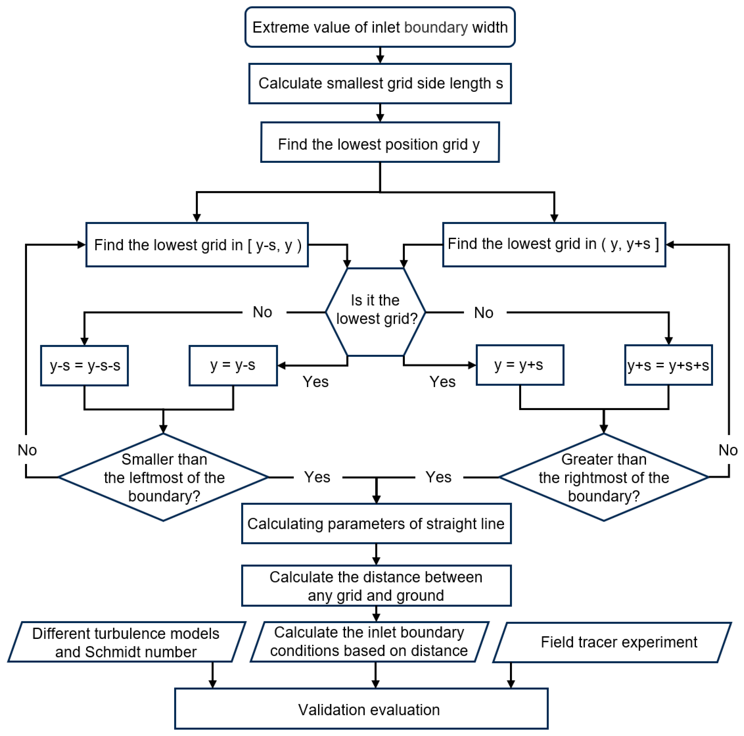
This section presents the enhancement of the Atmospheric Boundary Layer inlet boundary condition for uneven terrain, which is based on the default ABL inlet boundary condition. Initially, in Section 3.2, the $k-\epsilon$ turbulence model and the $k-\omega$ turbulence model are selected and introduced. Subsequently, as detailed in Section 3.1, numerical simulations are conducted. These simulations utilize both the improved and default ABL inlet boundary conditions, in combination with the two aforementioned turbulence models and five different turbulent Schmidt numbers. The computational results of each model are then evaluated against the data from the atmospheric pollutant tracer experiment, with the evaluation being carried out using the evaluation indicators presented in Section 3.3. In Section 3.4, the assessment systematically incorporates multiple exposure pathways to compute the Total Effective Dose Equivalent (TEDE). This comprehensive quantification framework serves as the foundation for subsequent evaluation of radionuclide impacts on both human health and ecological systems. The framework of the methods is depicted in Figure 3.

The choice of the $k-ϵ$ and $k-\omega$ turbulence models is grounded in their extensive application and efficacy in simulating turbulent flows across diverse engineering scenarios [47,48]. The $k-ϵ$ model is renowned for its robustness and is frequently employed in engineering practice. It has been proven to be reliable in handling a wide range of turbulent flow problems. On the other hand, the $k-\omega$ model demonstrates superior performance in predicting flow characteristics within regions characterized by high strain rates and rotational effects. These conditions are prevalent in uneven terrains, making the $k-\omega$ model particularly suitable for such uneven topographical situations.

3.1. Improved Atmospheric Boundary Layer Inlet Conditions Based on Uneven Terrain

In OpenFOAM-v2012, the atmBoundaryLayer boundary condition is included. The atmBoundaryLayer class is a base class for handling the inlet boundary conditions, providing log-law type ground-normal inflow boundary conditions for wind velocity and turbulence quantities for homogeneous, two-dimensional, dry-air, equilibrium and neutral atmospheric boundary layer modelling [49].

The improved Atmospheric Boundary Layer inlet boundary condition represents an augmentation of the default ABL inlet boundary condition, specifically tailored to account for the underlying surface of uneven terrain. The crux of this improvement lies in adjusting the relative height of the altitude $z$ at the center of any cell within the inlet boundary. Instead of measuring from the lowest altitude $G_{min}$, it is now measured as the relative height of $z$ to the reference altitude $G_{ref}$ projected onto the ground at that particular location.

When dealing with flat terrain, the two expressions, the original and the modified, are equivalent in meaning. Nevertheless, in the case of uneven terrain, the improved inlet boundary conditions offer a more precise reflection of the actual situation. In contrast, the default inlet boundary condition tends to over estimate the relative height of $z$. Consequently, the improved inlet boundary conditions subsume the default boundary conditions. In other words, the default inlet boundary conditions can be considered a proper subset of the improved inlet boundary conditions, as illustrated in

Table 1. Improved and default ABL comparison.

Parameter	Default ABL	Improved ABL
$u$	${\displaystyle \frac{u^{*}}{\kappa }}\left({\displaystyle \frac{z-G_{\min }-d+z_0}{z_0}}\right)$	${\displaystyle \frac{u^{*}}{\kappa }}\left({\displaystyle \frac{z-G_{ref}-d+z_0}{z_0}}\right)$
$k$	${\displaystyle \frac{{\left(u^{*}\right)}^2}{\sqrt{C_{\mu }}}}\sqrt{C_1\ln \left({\displaystyle \frac{z-G_{\min }-d+z_0}{z_0}}\right)+C_2}$	${\displaystyle \frac{{\left(u^{*}\right)}^2}{\sqrt{C_{\mu }}}}\sqrt{C_1\ln \left({\displaystyle \frac{z-G_{ref}-d+z_0}{z_0}}\right)+C_2}$
$\epsilon$	${\displaystyle \frac{{\left(u^{*}\right)}^3}{\kappa \left(z-G_{\min }-d+z_0\right)}}\sqrt{C_1\ln \left({\displaystyle \frac{z-G_{\min }-d+z_0}{z_0}}\right)+C_2}$	${\displaystyle \frac{{\left(u^{*}\right)}^3}{\kappa \left(z-G_{ref}-d+z_0\right)}}\sqrt{C_1\ln \left({\displaystyle \frac{z-G_{ref}-d+z_0}{z_0}}\right)+C_2}$
$\omega$	${\displaystyle \frac{u^{*}}{\kappa \sqrt{C_{\mu }}}}{\displaystyle \frac{1}{z-G_{\min }-d+z_0}}$	${\displaystyle \frac{u^{*}}{\kappa \sqrt{C_{\mu }}}}{\displaystyle \frac{1}{z-G_{ref}-d+z_0}}$

Where $u$ is speed profile $\left(\mathrm{m}/\mathrm{s}\right)$, $k$ is turbulent kinetic energy profile $\left({\mathrm{m}}^2/{\mathrm{s}}^2\right)$, $\epsilon$ is TKE dissipation rate profile $\left({\mathrm{m}}^2/{\mathrm{s}}^3\right)$, $\omega$ is specific dissipation rate profile $\left({\mathrm{m}}^2/{\mathrm{s}}^3\right)$, $u^{*}$ is Friction velocity $\left(\mathrm{m}/\mathrm{s}\right)$, $\kappa$ is von Kármán constant, $C_{\mu }$ is Empirical model constant, $z$ is coordinate component $\left(\mathrm{m}\right)$, $d$ is Ground-normal displacement height $\left(\mathrm{m}\right)$, $z_0$ is Aerodynamic roughness length $\left(\mathrm{m}\right)$, $C_1$ and $C_2$ are Curve-fitting coefficients.

.

To attain the aforementioned objective, the inlet boundary of the physical model now requires processing. This approach is applicable to the numerical simulation of the Atmospheric Boundary Layer within a domain that is approximately cuboidal, with the inlet boundary having an approximately rectangular shape. The process is divided into three steps:

(1)

Preliminary Work

Firstly, compute the width of the inlet boundary. Subsequently, determine the area of the smallest cell at the inlet boundary. Then, utilize the square root of the smallest cell area as the basis for the loop. Next, identify the cell with the lowest altitude within the inlet boundary (in the case of multiple cells having the same lowest altitude, any one can be chosen). Based on the altitude of this cell (specifically, the altitude at the cell center), divide the inlet boundary into two parts, namely the left-hand side and the right-hand side. Subsequently, perform individual loops on both parts to locate all the cells with the lowest altitude within the inlet boundary.

(2)

Identify the Lowest Cell

Once the loop commences, initially find the cell with the lowest altitude in the subsequent area. Then, determine whether it is the cell with the lowest altitude in the entire area. The criteria for this determination are whether its altitude is lower than that of the previous cell, or if its height is higher than the previous cell’s altitude but the elevation angle is less than 10°, as presented in Equation (1).

$$\theta =\arctan \left({\displaystyle \frac{\left|Z_{R\left(n+1\right)}-Z_{R\left(n\right)}\right|}{\left|Y_{R\left(n+1\right)}-Y_{R\left(n\right)}\right|}}\right)\times \frac{180°}{\pi }$$

(1)

$$k_{line}={\displaystyle \frac{Z_{L\left(n+1\right)}-Z_{L\left(n\right)}}{Y_{L\left(n+1\right)}-Y_{L\left(n\right)}}}$$

(2)

$$b=z_{L\left(n+1\right)}-k_{line}\times y_{L\left(n\right)}$$

(3)

$$G_{ref}=k_{line}\cdot Y+b$$

(4)

where $Z_m$ represents the z coordinate of point m, $Y_n$ represents the y coordinate of point n, $\theta$ represents the elevation angle, $k_{line}$ is the slope of the straight line between the two lowest points, and b is the intercept. $G_{ref}$ represents elevation of the cell projected to the surface.

The criterion for the elevation angle should be determined in accordance with the specific terrain undulations. In this instance, 10° is deemed appropriate. After the determination, save the values of the cell centers (x, y, z) of the cells that meet the requirements in an array. Subsequently, calculate the linear equation of the line connecting adjacent cell centers within the array. It is essential to record the parameters of the line: the slope $k$ and the intercept $b$, as shown in Equations (2) and (3).

(3)

Calculate the Inlet Boundary Conditions

Traverse all the cells at the inlet boundary. Then, based on the array consisting of the altitudes of the lowest cell centers obtained previously, determine the interval into which each cell falls. According to the linear parameter data of the interval, calculate the altitude of the cell and its projected altitude onto the ground, as shown in Equation (4). Subsequently, determine the relative height with respect to the cell center altitude, as depicted by the red line in Figure 4. Finally, substitute this relative height into the formula to calculate the inlet boundary conditions for the corresponding physical quantities, including velocity, turbulent kinetic energy, turbulence dissipation rate, and specific dissipation rate.

3.2. Governing Equations and Turbulence Modeling

In this subsection, we present the fundamental governing equations and the associated turbulence–closure frameworks. For a steady, incompressible Newtonian flow without external body forces, the Reynolds-averaged Navier–Stokes equations in conservative form can be written in Einstein summation notation as

$${\displaystyle \frac{\partial U_i}{\partial x_i}}=0$$

(5)

$$\frac{\partial \left(U_i{U}_j\right)}{\partial x_j}=-\frac{1}{\rho }\frac{\partial \overline{p}}{\partial x_i}+\frac{\partial }{\partial x_j}\left(\nu \frac{\partial U_i}{\partial x_j}-\overline{u_i^{\prime }{u}_j^{\prime }}\right)$$

(6)

where $U_i$, $U_j$ are the mean velocity components, $u_i^{\prime }$, $u_j^{\prime }$ are the fluctuating velocity components in the $x_i$, $x_j$ directions (i, j = 1, 2, 3). p is the pressure, $\nu$ is the kinematic viscosity, and $\rho$ is the density.

A prescription is needed for computing $-\overline{u_i^{\prime }{u}_j^{\prime }}$ for the calculation of all mean-flow properties. Assuming that the Boussinesq linear isotropic eddy-viscosity hypothesis is valid, the specific Reynolds-stress tensor is expressed by:

$$-\overline{u_i^{\prime }{u}_j^{\prime }}=2{\nu }_t{S}_{ij}-{\displaystyle \frac{2}{3}}k{\delta }_{ij}$$

(7)

where ${\nu }_t$ is the kinematic eddy viscosity ${\nu }_t=C_{\mu }{\displaystyle \frac{k^2}{\epsilon }}$, $k={\displaystyle \frac{1}{2}}\overline{u_i^{\prime }{u}_j^{\prime }}$ is the turbulence kinetic energy (TKE),

$$S_{ij}=\left({\displaystyle \frac{\partial U_j}{\partial x_i}}+{\displaystyle \frac{\partial U_i}{\partial x_j}}\right)$$

(8)

$S_{ij}$ is the strain rate tensor, and ${\delta }_{ij}$ is the Kronecker Delta function.

(a)

RNG $k-ϵ$

In this study, a realizable $k-ϵ$ turbulence model [50] was used. The modeled transport equations for TKE and the turbulence dissipation rate ($ϵ$) in the realizable k–ε model are,

$${\displaystyle \frac{\partial U_{j}k}{\partial x_j}}={\displaystyle \frac{\partial }{\partial x_j}}\left[\right(\nu +{\displaystyle \frac{{\nu }_t}{{\sigma }_k}}\left){\displaystyle \frac{\partial k}{\partial x_j}}\right]+P_k-\epsilon$$

(9)

$${\displaystyle \frac{\partial U_jϵ}{\partial x_j}}={\displaystyle \frac{\partial }{\partial x_j}}\left[\right(\nu +{\displaystyle \frac{{\nu }_t}{{\sigma }_k}}\left){\displaystyle \frac{\partial ϵ}{\partial x_j}}\right]+C_1{\displaystyle \frac{\epsilon }{k}}{P}_k-C_2{\displaystyle \frac{{\epsilon }^2}{k+\sqrt{\nu \epsilon }}}$$

(10)

where ${\sigma }_k$ = 1, ${\sigma }_{ϵ}$ = 1.2, and $C_2$ = 1.9.

The production of k is modeled as follows,

$$P_k={\nu }_t{S}^2,S=\sqrt{2S_{ij}{S}_{ij}}$$

(11)

The model coefficient C₁ is determined as follows,

$$C_1=max[0.43,{\displaystyle \frac{\eta }{\eta +5}}],\eta =S{\displaystyle \frac{k}{\epsilon }}$$

(12)

In contrast to the standard $k-ϵ$ model [32], $C_{\mu }$ in Equation (6) is not constant and is computed from

$$C_{\mu }={\displaystyle \frac{1}{A_0+A_S\frac{k{U}^{*}}{ϵ}}},U^{*}\equiv \sqrt{S_{ij}{S}_{ij}+{\mathsf{\Omega }}_{ij}{\mathsf{\Omega }}_{ij}},{\mathsf{\Omega }}_{ij}={\displaystyle \frac{1}{2}}({\displaystyle \frac{\partial U_i}{\partial x_j}}-{\displaystyle \frac{\partial U_j}{\partial x_i}})$$

(13)

The model constants $A_0$ and $A_s$ are given by

$$A_0=4.04,A_s=\sqrt{6}cos\varphi$$

(14)

$$\varphi ={\displaystyle \frac{1}{3}}co{s}^{-1}(\sqrt{6}W),W={\displaystyle \frac{S_{ij}{S}_{jk}{S}_{ki}}{{\tilde{S}}^3}},\tilde{S}=\sqrt{S_{ij}{S}_{ij}}$$

(15)

The superiority of the realizable $k-ϵ$ model over other $k-ϵ$ turbulence models has been reported in previous systematic validation studies for flow around buildings [51,52,53,54]. Notably, Yang et al. [55] concluded that the realizable $k-ϵ$ model provides more reasonable predictions of the turbulence intensity for the simulations of the swirling and separating flows around buildings than those with the use of the standard and RNG $k-ϵ$ models according to their CFD simulations and field measurements conducted to evaluate the wind resources available in an urban area.

(b)

$SSTk-\omega$

$${\displaystyle \frac{\partial \left(U_{j}k\right)}{\partial x_j}}={\displaystyle \frac{\partial }{\partial x_j}}\left(\left(\mu +{\alpha }_k{\mu }_t\right){\displaystyle \frac{\partial k}{\partial x_j}}\right)+G_k-{\displaystyle \frac{2}{3}}k{\displaystyle \frac{\partial u}{\partial x_j}}-{\beta }^{*}\omega k+S_k$$

(16)

$${\displaystyle \frac{\partial \left(U_j\omega \right)}{\partial x_j}}=\nabla \cdot \left(\left(\mu +{\alpha }_{\omega }{\mu }_t\right)\nabla \omega \right)+\gamma {\displaystyle \frac{G_k}{\nu }}-{\displaystyle \frac{2}{3}}\gamma \omega \left(\nabla \cdot u\right)-\beta {\omega }^2-\left(F_1-1\right)C{D}_{k\omega }+S_{\omega }$$

(17)

The blending function $F_1$ is a modifier for selecting $k-\omega$ or $k-ϵ$ turbulent model without user interaction. This function is zero away from the surface and switches to one inside the boundary layer:

$$F_1=\tan \mathrm{h}\left({\left(\min \left[\max \left({\displaystyle \frac{k^{1/2}}{{\beta }^{*}\omega y}},{\displaystyle \frac{500\nu }{y^2\omega }}\right){\displaystyle \frac{4\rho {\alpha }_{\omega 2}k}{C{D}_{k\omega }{y}^2}}\right]\right)}^4\right)$$

(18)

$$C{D}_{k\omega }=\max \left(2\rho {\alpha }_{\omega 2}{\displaystyle \frac{1}{\omega }}{\displaystyle \frac{\partial k}{\partial x_i}}{\displaystyle \frac{\partial \omega }{\partial x_i}},{10}^{-10}\right)$$

(19)

The turbulent kinematic viscosity ${\nu }_t$ is calculated as:

$${\nu }_t=a_1{\displaystyle \frac{k}{\max \left(a_1\omega ,b_1{F}_2\sqrt{2S_{ij}{S}_{ij}}\right)}}$$

(20)

$F_2$ is the second blending function:

$$F_2=\tan \mathrm{h}\left({\left[\max \left({\displaystyle \frac{2k^{1/2}}{{\beta }^{*}\omega y}},{\displaystyle \frac{500\nu }{y^2\omega }}\right)\right]}^2\right)$$

(21)

(c)

Convection–diffusion

The contaminant dispersion is modeled by a convection–diffusion equation:

$${\displaystyle \frac{\partial \left(U_{j}C\right)}{\partial x_j}}={\displaystyle \frac{\partial }{\partial x_j}}\left[\left({\displaystyle \frac{\nu }{Sc}}+{\displaystyle \frac{{\nu }_t}{S{c}_t}}\right){\displaystyle \frac{\partial C}{\partial x_j}}\right]$$

(22)

where $C$ is the concentration, $Sc$ is the Schmidt number, and $S{c}_t$ is the turbulent Schmidt number. The turbulent Schmidt number for the reference case is set to 0.7 as the default value in the software (see Tominaga and Stathopoulos [56]).

3.3. Model Evaluation

To delve deeper into the quantitative comparison of the disparities between numerical simulations and atmospheric dispersion tracer experiments, an evaluation method put forward by Hanna [57,58,59,60,61] is employed. This method serves to comprehensively evaluate the outcomes of two turbulence models, along with the improved and default Atmospheric Boundary Layer inlet boundary conditions. It has found extensive application in the research on pollutant dispersion model evaluation.

The performance of the model is assessed using several statistical metrics, including the Fractional Bias (FB), Geometric Mean Bias (MG), Geometric Variance (VG), Normalized Mean Square Error (NMSE), and the proportions of predictions falling within a factor of two (FAC2) and a factor of five (FAC5) of the observed values. These evaluation criteria are defined as follows:

$$FB={\displaystyle \frac{2\left(\overline{C_o}-\overline{C_p}\right)}{\left(\overline{C_o}+\overline{C_p}\right)}}$$

(23)

$$MG=\exp \left(\overline{\ln C_o}-\overline{\ln C_p}\right)$$

(24)

$$VG=\exp \overline{{\left(\ln C_o-\ln C_p\right)}^2}$$

(25)

$$NMSE={\displaystyle \frac{\overline{{\left(C_o-C_p\right)}^2}}{\overline{C_o{C}_p}}}$$

(26)

$$FAC2=0.5\le {\displaystyle \frac{C_p}{C_o}}\le 2.0$$

(27)

$$FAC5=0.2\le {\displaystyle \frac{C_p}{C_o}}\le 5.0$$

(28)

Here, the symbol $C_p$ stands for the predicted concentration, and $C_0$ represents the measured concentration. In the ideal scenario where the model can accurately predict the measured data, the performance indicators $FAC2$, $FAC5$, $MG$, and $VG$ all take on a value of 1. Conversely, $FB$ and $NMSE$ become zero. This indicates that a perfect prediction implies that the predicted values are in such close agreement with the measured values that these specific metrics reach their optimal or ‘perfect’ values, signifying minimal deviation between the model’s predictions and the real-world measurements.

3.4. Dose Calculation

After a nuclear facility accident, the population is exposed to radioactive materials in several ways: (1) external exposure from radionuclides deposited on the land (groundshine); (2) external exposure from radionuclides concentrated in the radioactive cloud (cloudshine); and (3) internal exposure from the intake of radionuclides [62].

These exposure pathways were considered in the assessment to calculate the Total Effective Dose Equivalent. TEDE is defined by the US Nuclear Regulatory Commission as a radiation dosimetry quantity used to monitor and control human exposure to radiation.

In this study, TEDE values were calculated using Computational Fluid Dynamics methodology for dose assessment. As the deposition effects were excluded from the computational framework, the analysis focused exclusively on evaluating the impact of radionuclide air concentrations on both human exposure and environmental contamination.

The calculation procedure is explained through a series of equations listed below.

Inhalation dose can be calculated using Equation (29):

$$D_{inh}=C_A\times V_B\times D{C}_{inh}\times \left(F_{in}\times C_{in}+F_{out}\times C_{out}\right)$$

(29)

where $D_{inh}$ is an inhalation dose $\left({\mathrm{S}}_{\mathrm{V}}\right)$; $C_A$ corresponds to the air concentration $\left(\mathrm{B}\mathrm{q}/{\mathrm{m}}^3\right)$; $V_B$ is a breathing rate $\left({\mathrm{m}}^3/\mathrm{d}\mathrm{a}\mathrm{y}\right)$; $D{C}_{inh}$ relates to radionuclide specific dose conversion factor for inhalation $\left({\mathrm{S}}_{\mathrm{V}}/\mathrm{B}\mathrm{q}\right)$; $F_{in}$ and $F_{out}$ are fractions of time spent indoor and outdoor, respectively; $C_{in}$ and $C_{out}$ are indoor and outdoor reduction factors.

External cloud dose is calculated using the following relation, Equation (30):

$$D_{cloud}=C_a\times DC{F}_{cloud}\times {\displaystyle \sum f_i}\times c_j$$

(30)

where $D_{cloud}$ is a cloudshine dose $\left({\mathrm{S}}_{\mathrm{V}}\right)$; $C_a$ is the air concentration $\left(\mathrm{B}\mathrm{q}/{\mathrm{m}}^3\right)$; $DC{F}_{cloud}$ relates to a cloudshine dose conversion factor $\left({\mathrm{S}}_{\mathrm{V}}\times {\mathrm{m}}^3/\mathrm{B}\mathrm{q}\times \mathrm{s}\right)$; and $f_i$ fraction of time staying at outdoor location $i$ and $c_j$ is a correction coefficient for the gamma dose rate at outdoor location $i$.

TEDE doses are then calculated as the sum of the effective dose equivalent (for external exposure) and the committed effective dose equivalent (for internal exposures) using Equation (31):

$$TEDE=D_{inh}+D_{cloud}$$

(31)

Table 2. Typical Radionuclide Parameters in Airborne Effluents from Four Types of Nuclear Facilities.

Nuclides	Half-Life (Year)	Inhalation Dose Conversion Factor (Sv·m3/Bq·s)	Air Submersion Dose Rate Coefficient (Sv·m3/Bq·s)	Activity (Bq/Year)	Breathing Rate (m3/Day)
3$H$	12.35	1.80 × 10−11	3.80 × 10−20	4.09 × 1015	19.2
14$C$	5730	6.20 × 10−12	3.86 × 10−17	1.86 × 1011	19.2
85$Kr$	10.73	-	6.67 × 10−16	6.66 × 1016	19.2
129$I$	1.6 × 107	9.60 × 10−8	2.54 × 10−16	3.31 × 108	19.2

summarizes the radiological parameters of four nuclides (³$H$, ¹⁴$C$, ⁸⁵$Kr$ and ¹²⁹$I$), including their half-lives, inhalation-derived effective dose coefficients for members of the public, air submersion effective dose rate coefficients for reference persons, breathing rate and annual emission quantities [63].

4. Case Setup

4.1. Computational Domain

The present study focuses primarily on the effects of uneven terrain on atmospheric flow and dispersion. Consequently, ancillary buildings surrounding the core nuclear facilities are not explicitly meshed; instead, their influence is represented via a surface roughness model coupled with near-ground wall functions. High-resolution topographic data are obtained from the 1 arcsecond Shuttle Radar Topography Mission (SRTM) database provided by the USGS, which offers a horizontal resolution of 30 m [64]. These raw elevation data are subsequently processed and refined to match the actual site morphology before grid generation.

Domain dimensions follow the Best Practice Guidelines of Franke et al. [65] and Tominaga et al. [66]. In accordance with Franke’s recommendation [67], the vertical extent reaches ten times the maximum building height (H) above ground level, and the downstream length from the facility cluster to the outlet is set at 15H. Beyond the primary 2.0 km × 2.4 km facility footprint, the computational domain extends 1.4 km (14H) upwind and 7.4 km (74 H) downwind of the tallest structure (H = 100 m). Lateral extents are 6.0 km (6 H) on the left and 6.5 km (6.5 H) on the right to encompass tracer sampling locations. Given that the field tracer experiment was conducted with the wind blowing from 42° south of west, the physical model is rotated 48° clockwise so that the prevailing flow aligns with the X-axis. The geometric configuration of the computational domain is illustrated in Figure 5. The resulting blockage ratio is 1.125%, well below the 5% threshold of COST Action guidelines. This configuration thus balances computational tractability with the accuracy required for reliable diffusion and dispersion predictions [68].

4.2. Mesh Generation and Sensitivity Test

The grid-independence study was conducted using four unstructured meshes—denoted Basic, Medium, Fine, and Extra-Fine—with cell counts of 11,745,126; 18,495,206; 26,839,849; and 33,247,450, respectively. Figure 6 compares the mean velocity profiles in the along-wind direction at two key elevations (the chimney base and chimney top). Notably, the Basic mesh delivers velocity predictions nearly identical to those of the Extra-Fine mesh at both heights, indicating rapid convergence with relatively coarse resolution.

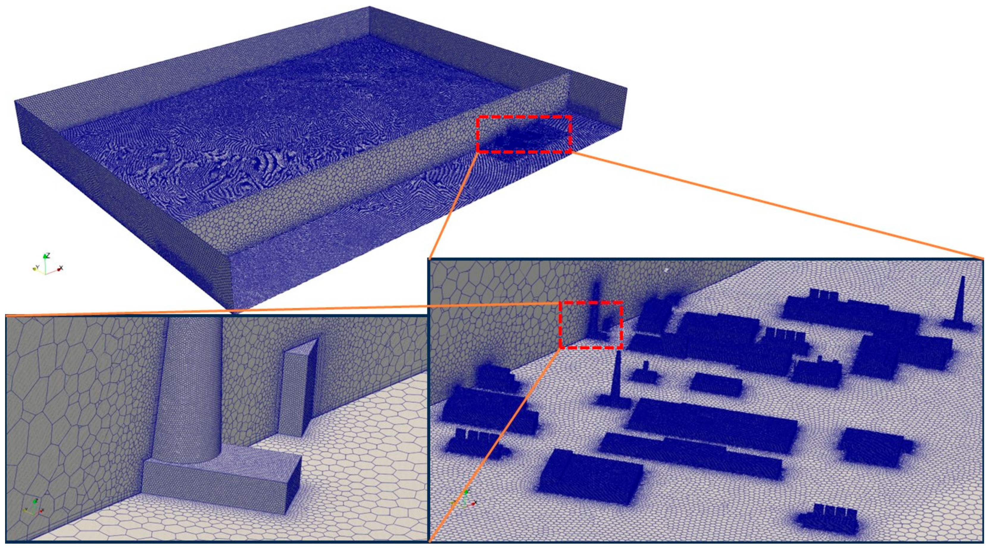
All unstructured meshes were generated in ANSYS Fluent Meshing (version 2022 R1) using polyhedral elements to maximize cell quality while maintaining a manageable total count. Based on the sensitivity results, the Fine mesh (26,839,849 cells) was selected as the most cost-effective option, exhibiting an average non-orthogonality of 10.27°. The near-surface region employs prismatic layers that conform to terrain contours, created via ANSYS PolyHexCore meshing to ensure a smooth transition into the hexahedral core domain. Local refinements of 0.1 m at the chimney outlet and 1 m around buildings and terrain features (with gradual grading from 1 m to 20 m elsewhere) capture steep gradients without unduly inflating the cell count. As shown in Figure 7, the mesh density increases progressively upward (along the Z-axis above structures) and outward in the X–Y plane, with a maximum expansion ratio of 1.2 to balance accuracy and efficiency.

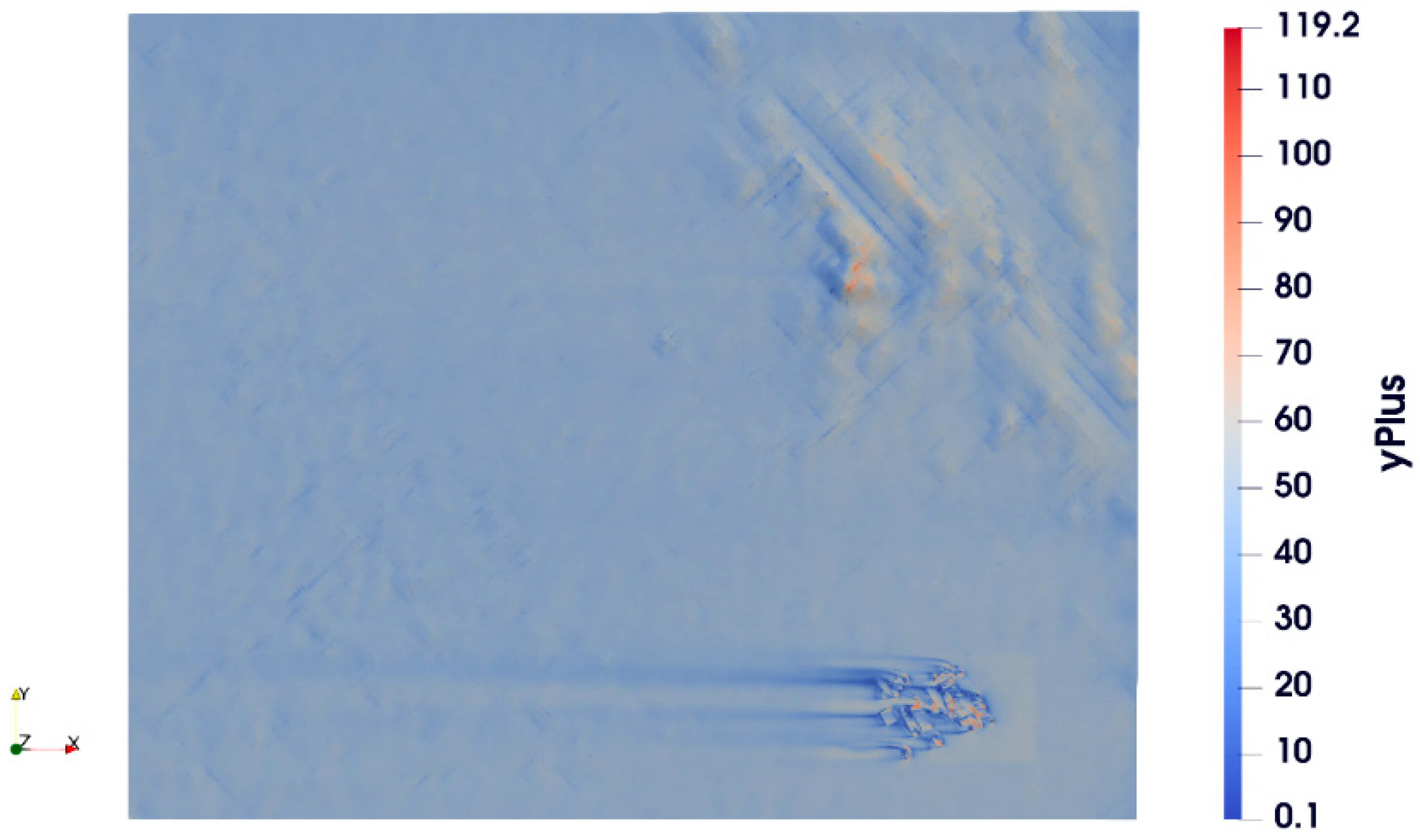
To accurately capture near-wall flow characteristics, inflation layers were incorporated across all surfaces within the computational geometry, including both terrain and structural elements. The initial off-wall cell height was set to approximately 6.27 × 10⁻³ m, ensuring that the first grid point resides within the viscous sublayer. This configuration yielded average dimensionless wall distances ($y^{+}$) of approximately 41.03 for building surfaces and 39.16 for terrain surfaces. A comprehensive grid convergence study was conducted to balance computational efficiency with simulation accuracy.

As illustrated in Figure 8, the mesh was refined in regions encompassing the ground and buildings to ensure $y^{+}$ values met the requirements for accurate solution computation. The distribution of $y^{+}$ values indicates that the majority are below 100, with only localized areas—such as elevated hilltops and certain building regions—exceeding this threshold, yet remaining below 119. This refinement strategy ensures that the mesh adequately resolves the boundary layer, thereby enhancing the fidelity of the simulation results.

4.3. Simulation Setup

In this study, wind flow simulations were conducted using the OpenFOAM (version 2012) toolbox, an open-source Computational Fluid Dynamics software package [69]. The incompressible, three-dimensional, steady-state Reynolds-Averaged Navier–Stokes equations were solved using the finite volume method. Turbulence was modeled with the realizable $k-ϵ$ and $SSTk-\omega$ turbulence model [51].

The inlet wind profile was prescribed using a logarithmic law, calibrated against field measurement data. The reference wind speed was specified at the building height $U_h=5.66\mathrm{m}/\mathrm{s}$, with a surface roughness length of $Z_0=0.013\mathrm{m}$. A tracer gas was continuously released from a point source located 3 m above ground level, within the chimney structure. The emission rate was $q=5.03\times {10}^{-4}{\mathrm{m}}^3/\mathrm{s}$, and the initial gas concentration was $C_{gas}=1\times {10}^6\mathrm{p}\mathrm{p}\mathrm{m}$. The measured concentrations $C$ were normalized by a reference concentration $C_0={\displaystyle \frac{C_{gas}q}{H^2{U}_H}}$ to facilitate comparison and analysis. The specific parameter settings for the boundary conditions are summarized in

Table 3. Parameter settings of boundary conditions.

Parameter	Uh= 100 m m/s	Z0 m	q m3/s	Cgas ppm
Value	5.66	0.013	$5.03\times {10}^{-4}$	$1\times {10}^6$

.

Boundary conditions were assigned as follows: a pressure outlet condition was applied at the domain outlet, symmetry conditions were imposed on the top and lateral boundaries, and no-slip wall conditions were specified for both the ground and building surfaces. All simulations were carried out at full scale (1:1 geometric ratio).

The airflow field was computed using the simpleFoam solver, which is based on the Semi-Implicit Method for Pressure-Linked Equations (SIMPLE) algorithm and solves Equations (5)–(15). Based on the steady-state velocity field, the tracer gas concentration field was then obtained by solving Equation (22). Spatial discretization employed the central differencing scheme for both gradient and Laplacian terms. For divergence terms, a second-order upwind scheme was used for $U$, while the Van Leer scheme was applied to $k$, $ϵ$, and $\omega$. The central differencing scheme was again used for $C$. All numerical schemes ensured second-order accuracy in space. The convergence criterion for all residuals was set to ${10}^{-4}$.

The numerical modeling of radionuclide dispersion incorporated two distinct inlet boundary conditions derived from meteorological datasets, specifying wind velocities of 2.5 m/s and 4.21 m/s at a 10 m reference height. Source term initialization involved temporal downscaling of annual emission inventories to second-by-second flux rates at boundary nodes. The simulated dispersion patterns were subsequently annualized through temporal scaling algorithms to establish Total Effective Dose Equivalent projections, enabling systematic evaluation of long-term radiological impacts.

5. Results and Discussion

5.1. SF6 Concentrations of Atmospheric Dispersion Tracer Experiments

Following the atmospheric dispersion tracer experiment, a gas chromatograph was employed to analyze all sampling bags. Subsequently, experimental data processing was carried out to determine the $S{F}_6$ concentration at each sampling point. The data were normalized by comparing them with the background tracer gas concentration. Using the Triangulation with Linear Interpolation method in Surfer software [70,71,72,73], the data were further processed to obtain the spatial distribution characteristics of the concentration based on the sampling points, as depicted in Figure 9.

During the experimental setup, the sampling points were arranged in anticipation of an easterly wind. However, during the field test, the actual average wind direction was $42°$ south of west, nearly southwest. This deviation in wind direction resulted in a ground-based distribution of the tracer that had some overlap with, but did not fully coincide with, the on-site arranged points.

Overall, the spatial distribution of the concentration exhibits a gradual decline from the southeast to the northwest. Given that the main wind direction was $42°$ south of west, and the sampling points in the field experiment were set from $50°$ south of west to $70°$ north of south, the concentration at all sampling points along Ray 1 and some along Ray 2 was relatively high.

The normalized concentrations spanned from 1.45 to 88.21. The tracer’s maximum concentration, 88.21, was recorded at sampling point D1. This was succeeded by sampling points C1, E1, and F1, which had relatively elevated concentrations of 34.25, 11.36, and 7.97, respectively. Excluding these sampling points with higher tracer gas concentrations, the concentrations at the remaining points were within five times the background levels.

5.2. Comparison of Different Inlet Boundary Conditions

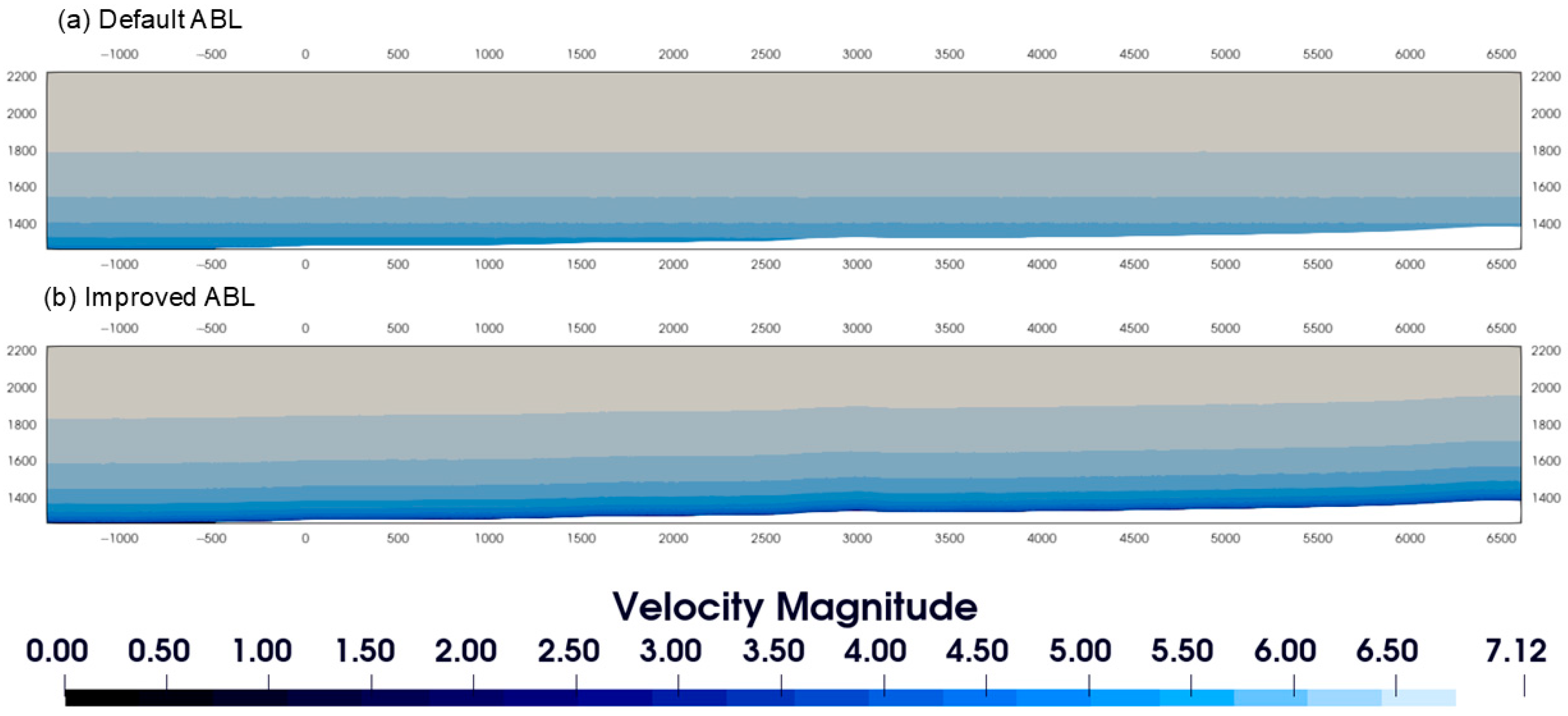
Figure 10 compares the velocity profiles between the default atmospheric boundary layer inlet boundary condition and the modified ABL inlet boundary condition over uneven terrain. The inlet wind speed distribution ranges from 0 to 7.12 m/s, represented by a color gradient transitioning from dark blue to light blue and finally to off-white. In Figure 10a, which illustrates the default ABL inlet boundary condition, the velocity distribution clearly demonstrates parallelism with the horizontal ground plane. Lower wind speeds are observed near the surface in the left section of the inlet boundary (lower elevation region), whereas higher wind speeds prevail near the surface in the right section (higher elevation region). The velocity magnitudes remain elevated from the surface to the model top. In contrast, Figure 10b presents the modified ABL inlet boundary condition, where the velocity distribution exhibits strong dependence on the terrain surface contour. Notably, surface wind speeds approach 0 m/s across both low- and high-elevation regions of the inlet boundary.

The distinct velocity distributions between these two ABL inlet boundary conditions, particularly the significant discrepancies near the surface, exert substantial impacts on numerical simulation outcomes. This discrepancy arises from fundamental differences in reference height determination. The default ABL boundary condition calculates relative height based on the lowest point within the entire inlet boundary domain. Conversely, the modified ABL boundary condition incorporates local elevation differences by utilizing projection points at arbitrary locations. Consequently, the modified ABL boundary condition demonstrates enhanced physical accuracy in simulating flow over uneven terrain, yielding more reliable predictions of near-surface wind behavior.

5.3. Comparative Evaluation of Different Simulation Results and SF6 Leakage Experiment

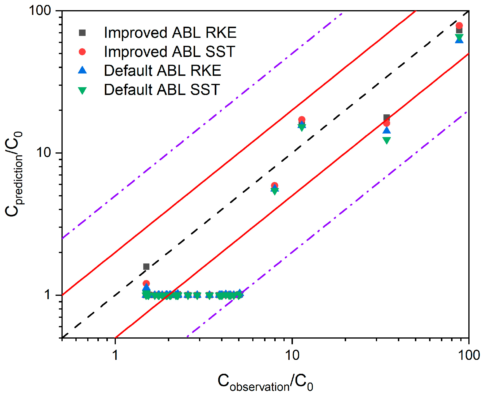
The outcomes of the six evaluation metrics for the four simulations are shown in

Table 4. Summary of the performance evaluation results of the different models and ABL.

Model	ABL	FB	MG	VG	NSME	FAC2	FAC5
RKE	Improved	0.4519	1.2325	1.0447	0.0928	0.4412	1
SST	Improved	0.4223	1.1488	1.0194	0.0772	0.4118	1
RKE	Default	0.5647	1.4476	1.1466	0.2053	0.4118	1
SST	Default	0.5524	1.3681	1.1032	0.1763	0.4118	1

. And Figure 11 depicts the ratio of the tracer gas concentration $C_0$ from the atmospheric dispersion tracer experiment to the background value $c_0$ on the horizontal axis, and the ratio of the numerical simulation value $c_p$ to the background value on the vertical axis. This graph is constructed using the tracer gas concentration data from the atmospheric dispersion tracer experiment and the concentration results of four numerical simulation scenarios. Points where the tracer gas concentration from the experiment matches the numerical simulation result lie on the line $c_p/c_0=1$, represented by the black dashed line in the figure. This indicates a high degree of agreement between the numerical simulation and the atmospheric dispersion tracer experiment results. The two red lines signify FAC2, meaning that the area enclosed by these lines corresponds to concentrations that are $1/2$ to 2 times the values obtained from the atmospheric dispersion tracer experiment, suggesting an acceptable match with the numerical simulation results. Similarly, the two purple dashed lines represent FAC5, encompassing concentrations ranging from $1/5$ to 5 times the atmospheric dispersion tracer experiment values, which indicates an acceptable range for the numerical simulation results.

As can be seen from Figure 11, all four simulation results are within the area between the two purple lines. Specifically, 41.18% of the points are between the two red lines, yet there are relatively few points close to the black dashed line. The reason for the clustering of many predicted values around a particular line is that in the simulation, the background values of the tracer at many points far from the pollutant diffusion center are dominant. Nevertheless, in the atmospheric dispersion tracer experiment, due to the uneven terrain, wind field variations, and turbulence effects, these sampling points are actually affected by contamination, leading to tracer gas concentrations higher than the background values. Points with higher tracer gas concentrations that cluster around the black line suggest reasonably accurate predictions, although some values may be over- or underestimated. However, the majority of sampling points with tracer gas concentrations are below the black dashed line, indicating that the concentrations simulated by the four models are lower than the tracer gas concentrations observed in the atmospheric dispersion tracer experiment.

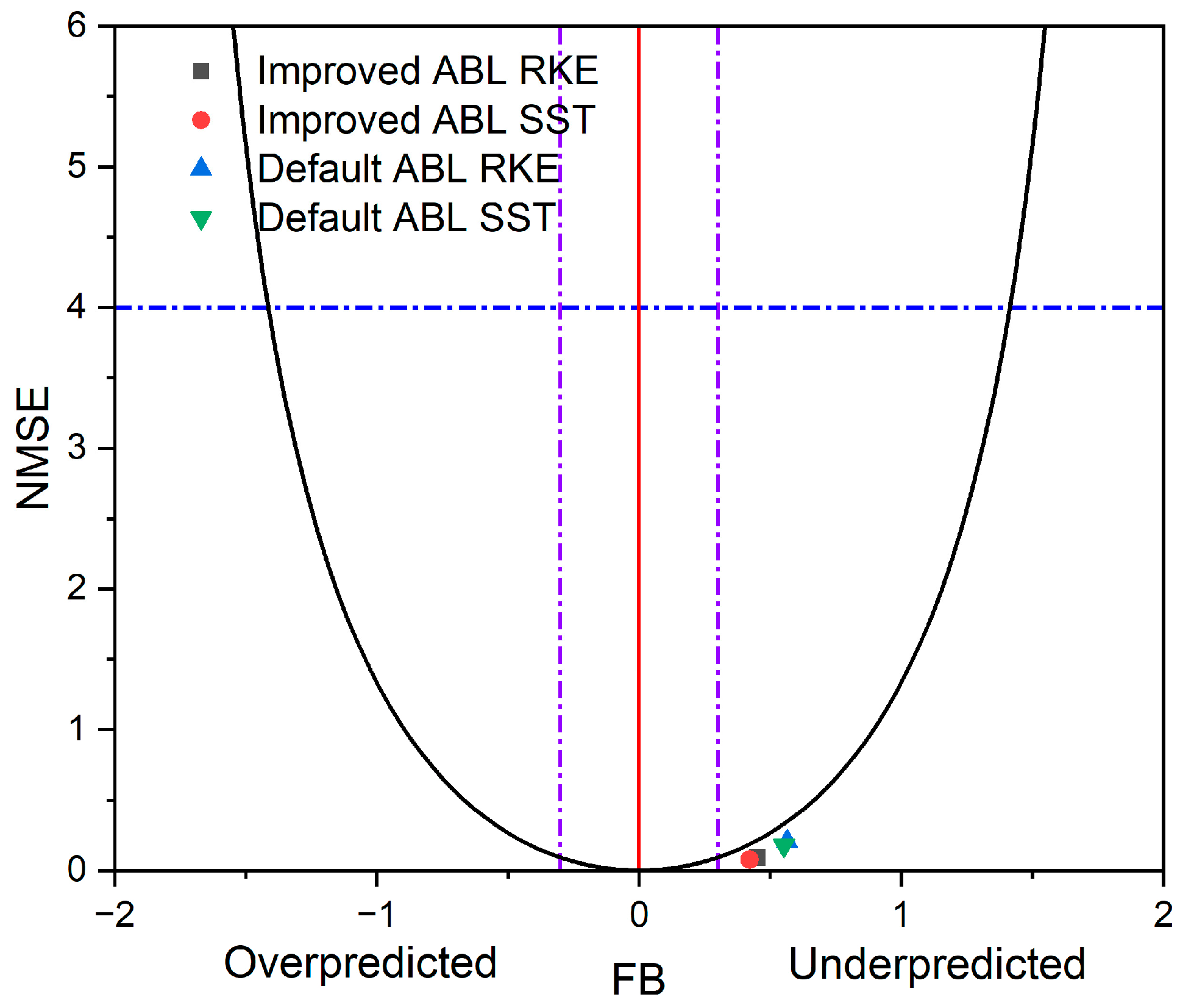
Upon examination of Figure 12, it becomes evident that none of the four cases lie within the optimal acceptance range of the Fractional Bias (FB). All the predicted values are lower than the measured ones; however, they are in close proximity to the boundary value of 0.3. The Normalized Mean Square Error (NMSE) indicators for all four cases are less than 4, a result that can be regarded as satisfactory.

Among these, the results denoted by red dots, corresponding to the Improved ABL SST model, stand out as the most favorable across the four cases. Next in line are the results represented by black dots, which pertain to the Improved ABL RKE model. Subsequently, the results indicated by green dots for the Default ABL SST model follow, and lastly, the results represented by blue dots for the Default ABL RKE model. Moreover, the results of the two Improved ABL cases exhibit similarity and demonstrate superiority over those of the Default ABL cases.

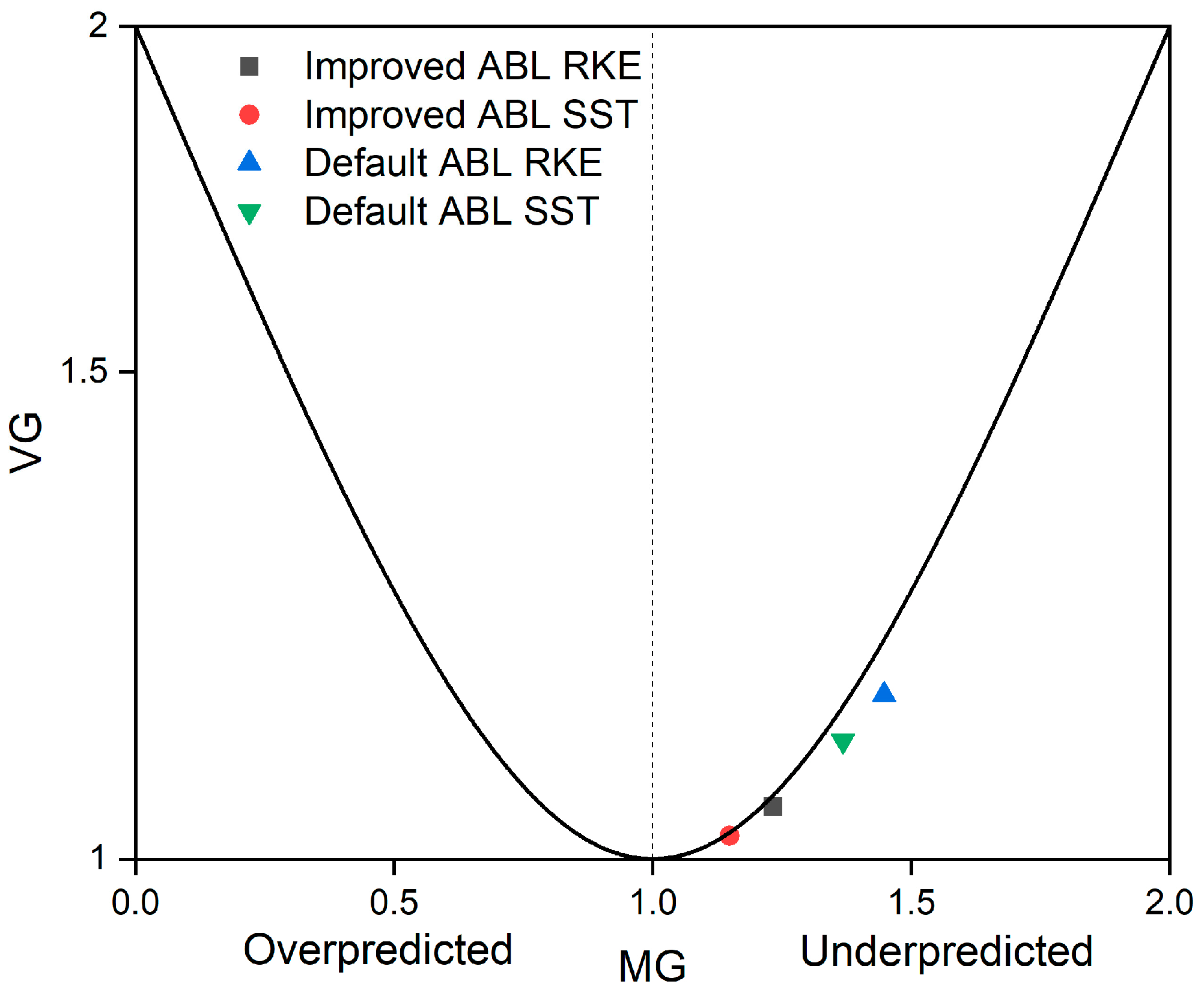
Figure 13 presents the MG-VG plot of tracer gas concentrations at different sampling points of numerical simulations and the atmospheric dispersion tracer experiment. In the plot, the point (1,1) represents the ideal point for the model. The results suggest that the closer the model is to this point, the higher the prediction accuracy of the selected turbulence model.

Analogous to the results in the FB-NMSE plot, the predicted values for all four cases are lower than the measured values. Nevertheless, they are close to the parabolic curve and not far from the ideal point. The results consistently demonstrate that the Improved ABL SST model performs the best, followed by the Improved ABL RKE model. Both of these outperform the latter two, namely the Default ABL SST and Default ABL RKE models.

In summary, considering its superior performance in the evaluation metrics among the four models, we select the Improved ABL SST model to predict the dispersion of pollutants under uneven terrain conditions.

5.4. Velocity and Turbulent Kinetic Energy of the Approaching Boundary Layer

To more effectively contrast the differences between the improved and default ABL inlet boundary conditions within uneven terrain environments, four vertical lines were established at two locations: the center of the factory area (at a lower altitude) and at high-altitude inlet locations. These lines were specifically positioned at distances of 500, 1000, and 1500 m from the inlet and the chimney release positions, as illustrated in Figure 14.

This study concentrated on examining the distribution of velocity and turbulent kinetic energy with height along these lines. The aim was to comprehend the disparities in ABL inlet boundary conditions between the improved and default configurations in uneven terrain settings. To offer a more intuitive portrayal of the terrain environment, different colors were employed. Progressively deeper shades of red signify increasing elevations, whereas increasingly darker shades of blue denote decreasing elevations. The elevation of the uneven terrain varies from a minimum of 1227 m to a maximum of 1394 m.

As shown in Figure 15, velocity profiles from two distinct inlet boundary conditions at two locations (x = 0 m and x = 3 km) are extracted for comparative analysis. The red and dark blue curves represent velocity profiles of the modified atmospheric boundary layer inlet boundary condition at x = 0 m and x = 3 km, respectively. The green and brown curves denote velocity profiles of the default ABL inlet boundary condition at x = 0 m and x = 3 km, while the purple and blue curves indicate the percentage difference in velocity magnitudes between the two boundary conditions at these positions.

The modified velocity profiles exhibit near-surface wind speeds approaching 0 m/s, whereas the default profiles maintain surface velocities exceeding 2 m/s. The velocity discrepancy between the two boundary conditions gradually decreases with increasing height. Variations in surface elevation at different inlet positions further influence the magnitude of velocity differences. These results demonstrate that the modified ABL inlet boundary condition primarily addresses significant velocity errors near the surface in numerical simulations.

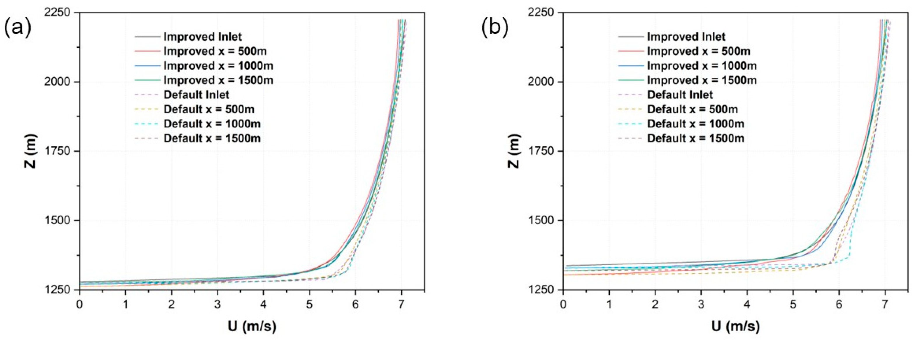
Figure 16 depicts the variation in velocity with height for both the improved and default ABL inlet boundary conditions at low and high altitudes. In Figure 16a, under low-altitude inlet conditions, it is evident that the default model displays higher velocities and greater accelerations near the ground in comparison to the improved model. The four curves of the improved model are closely grouped together, while there are subtle distinctions among the four curves of the default model. In Figure 16b, at high-altitude inlet conditions, the differences in velocity and acceleration between the default and improved models are more pronounced than at low-altitude conditions. The four curves of the improved model still exhibit a similar trend with only minor variations. However, the four curves of the default model show larger discrepancies and deviate more significantly from the improved model. Overall, the default model generally predicts higher velocities than the improved model, especially at high-altitude inlet conditions. This indicates that the default model overestimates velocities as a result of its incomplete consideration of relative heights.

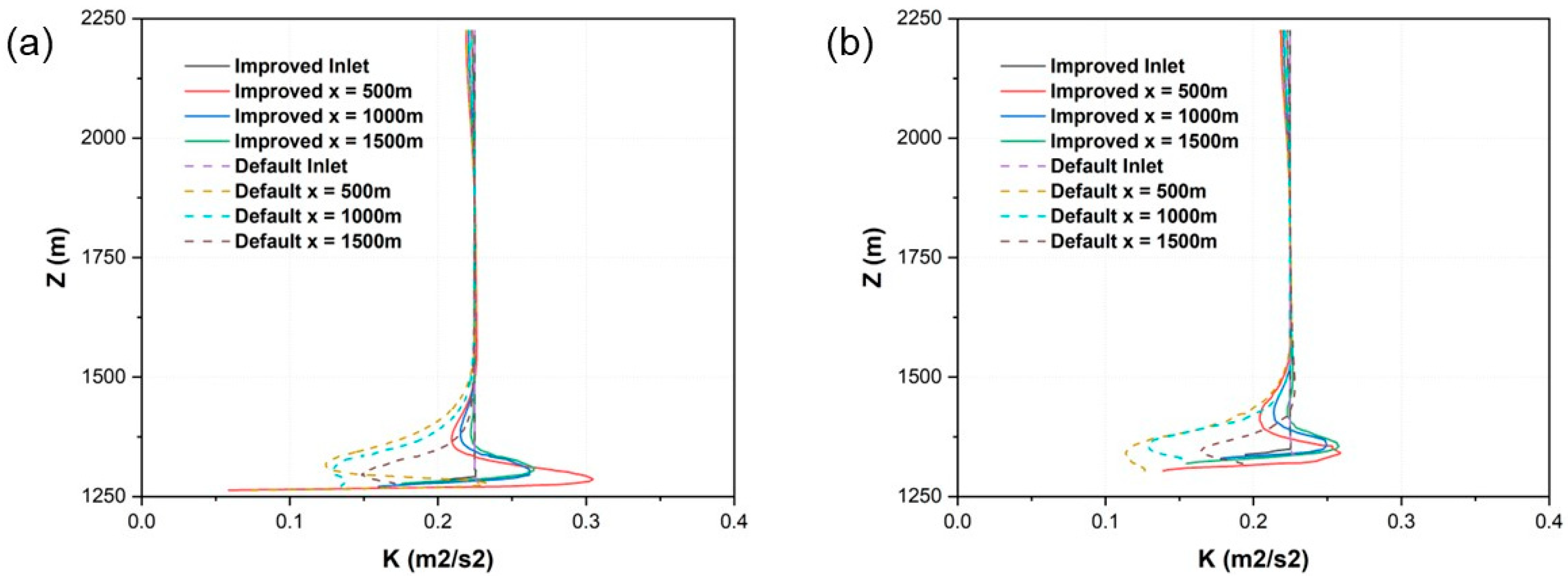
Figure 17 demonstrates the distribution of turbulent kinetic energy with respect to height for both the improved and default ABL inlet boundary conditions at low and high altitudes. In Figure 17a, the red line representing the improved model stands out from the rest. This is because it is in close proximity to buildings, leading to substantial changes. The other three solid lines of the improved model are closely grouped, suggesting a relatively stable pattern of variation. Conversely, the four dashed lines of the default model display more significant differences among themselves and have lower values when compared to the improved model.

In Figure 17b, the four profiles of turbulent kinetic energy for the improved model merge more smoothly than those of the default model, which have more distinct profiles. Nevertheless, due to the characteristics of turbulent models, the uneven terrain, and the unrealistic inlet turbulent kinetic energy profiles, none of these models can maintain highly consistent profiles.

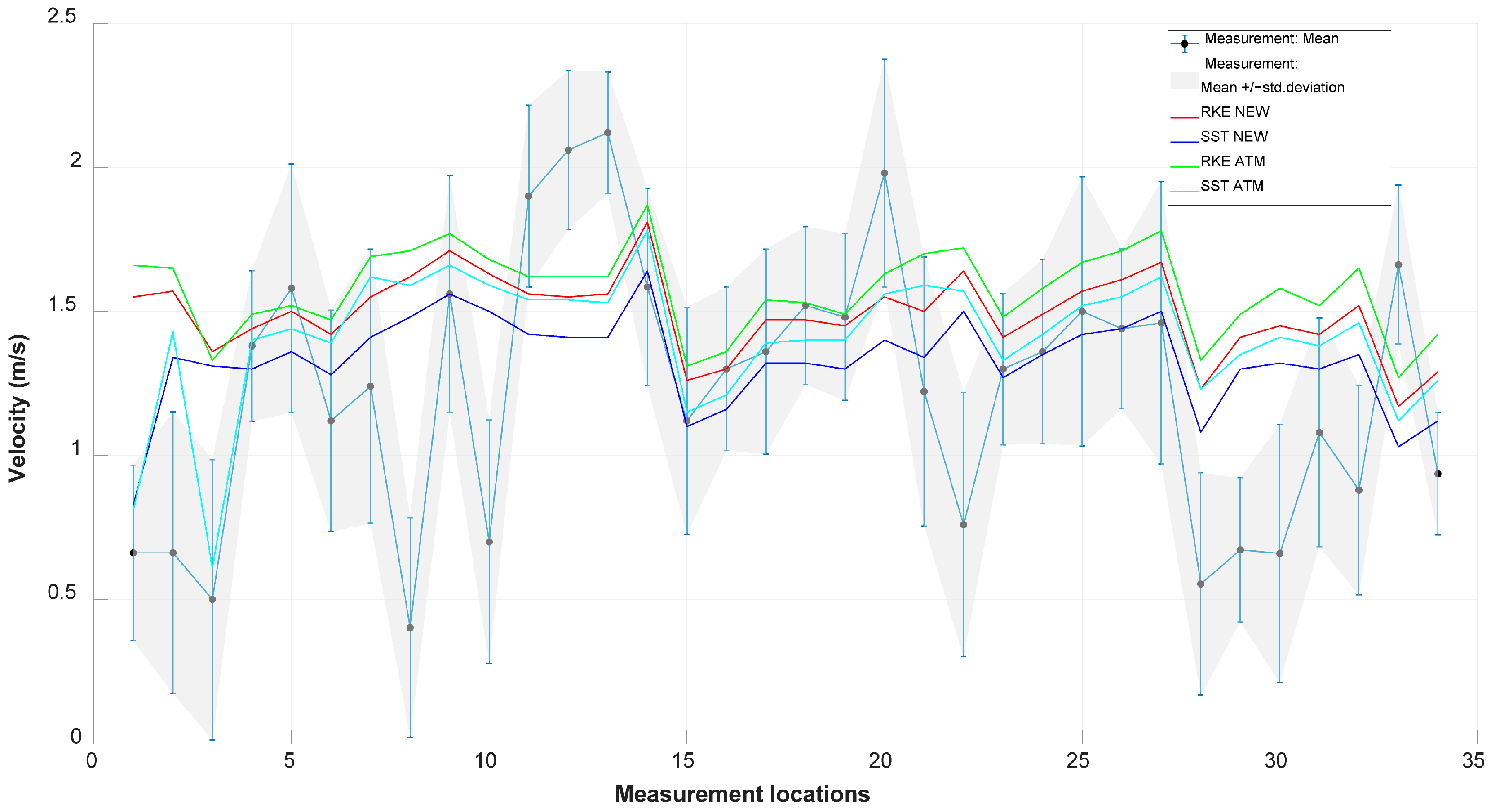
Figure 18 displays the wind velocity measurements with standard deviations at 34 sampling locations from an atmospheric diffusion tracer experiment, along with corresponding numerical simulation results obtained using four turbulence models with distinct inlet boundary conditions. Experimental wind speeds ranged from 0.0 to 2.3 m/s, whereas the simulated values exhibited a narrower distribution between 0.5 and 2.0 m/s. The chromatic representation employs red, blue, green, and cyan curves to denote the RKE NEW, SST NEW, RKE ATM, and SST ATM models, respectively.

Comparative analysis reveals that: (1) RKE-based models consistently generate higher wind velocities than their SST counterparts; (2) NEW boundary condition implementations yield superior velocity predictions compared to ATM configurations; (3) The SST NEW model demonstrates optimal agreement with experimental observations, establishing it as the most effective modeling approach among those evaluated.

5.5. Comparison of Contours at Height of 10 M from the Ground

Figure 19 depicts a comparison of the velocity contour lines at a height of 10 m above the ground for both the improved and default ABL inlet boundary conditions. Generally, the default model yields slightly higher velocities compared to the improved model. This is particularly evident in regions where buildings impede the wind flow, especially in areas with relatively large intervals between buildings. The improved model, on the other hand, exhibits lower velocities in the spaces between buildings. This can be ascribed to the disparities in the velocity profiles at the inlet.

To accentuate the velocity differences between the two models, Figure 19c presents the contour lines of the absolute velocity difference between the improved and default ABL inlet boundary conditions. This graph offers a more intuitive visualization, revealing that the maximum velocity difference between buildings can reach 4.1 m/s, and in numerous areas, the differences are up to 2 m/s.

Figure 20 presents a comparison of the contour lines of turbulent kinetic energy at a height of 10 m above the ground for both the improved and default ABL models. In comparison to the improved model, the default model demonstrates higher levels of turbulent kinetic energy behind numerous buildings, and this is particularly prominent in the spaces between buildings.

As can be clearly seen from Figure 20c, the difference in turbulent kinetic energy between buildings attains a maximum value of 1. Moreover, in many regions behind the buildings, the differences reach up to 0.5.

Figure 21 showcases the contour lines of the normalized tracer gas concentration at a height of 10 m above the ground for both the improved and default ABL models. It is apparent that elevated concentrations exist within roughly two factory lengths behind the chimney.

To emphasize the disparities between the two models, Figure 21c reveals that, in comparison to the default model, the improved model exhibits more concentrated aggregation within one factory length. This phenomenon occurs because the lower velocity in the improved model causes a delay in pollutant dispersion, thereby resulting in a higher degree of concentration aggregation.

Notably, the improved model aligns more closely with the simulated results than the default model. The presence of high pollutant concentrations in the improved model contributes to a more conservative and safer assessment of pollutant dispersion predictions.

5.6. Comprehensive Evaluation of Pollutant Diffusion Results with Different SCHMIDT Numbers

As depicted in Figure 22, notable differences in the results arise due to six distinct turbulent Schmidt numbers, which range from 0.3 to 1.3.

In Figure 22a, where the ideal value is 1, it can be observed that the average of FAC2 across the six Schmidt numbers is approximately 0.4. The best performance occurs when the turbulent Schmidt number is 0.5. Regarding FAC5, it approaches 1 in all cases, with the most favorable performance seen at turbulent Schmidt numbers of 0.5 and 0.7.

In Figure 22b, with an ideal value of 0, the Normalized Mean Square Error (NMSE) increases as the turbulent Schmidt number rises. The results are relatively more favorable at turbulent Schmidt numbers of 0.3 and 0.5. The Fractional Bias (FB) initially decreases and then increases with the increase in the turbulent Schmidt number. The optimal value is at 0.5, followed by 0.7 and 0.3.

In Figure 22c, where the ideal value is 1, the Geometric Mean (MG) increases with an increasing turbulent Schmidt number, reaching its optimum at a turbulent Schmidt number of 0.5. The Geometric Variance (VG) initially decreases and then increases as the turbulent Schmidt number increases. The best performance is observed at a turbulent Schmidt number of 0.5, followed by 0.7. In conclusion, the optimal turbulent Schmidt numbers for this model are 0.5 and 0.7.

5.7. Radiological Dose Calculations

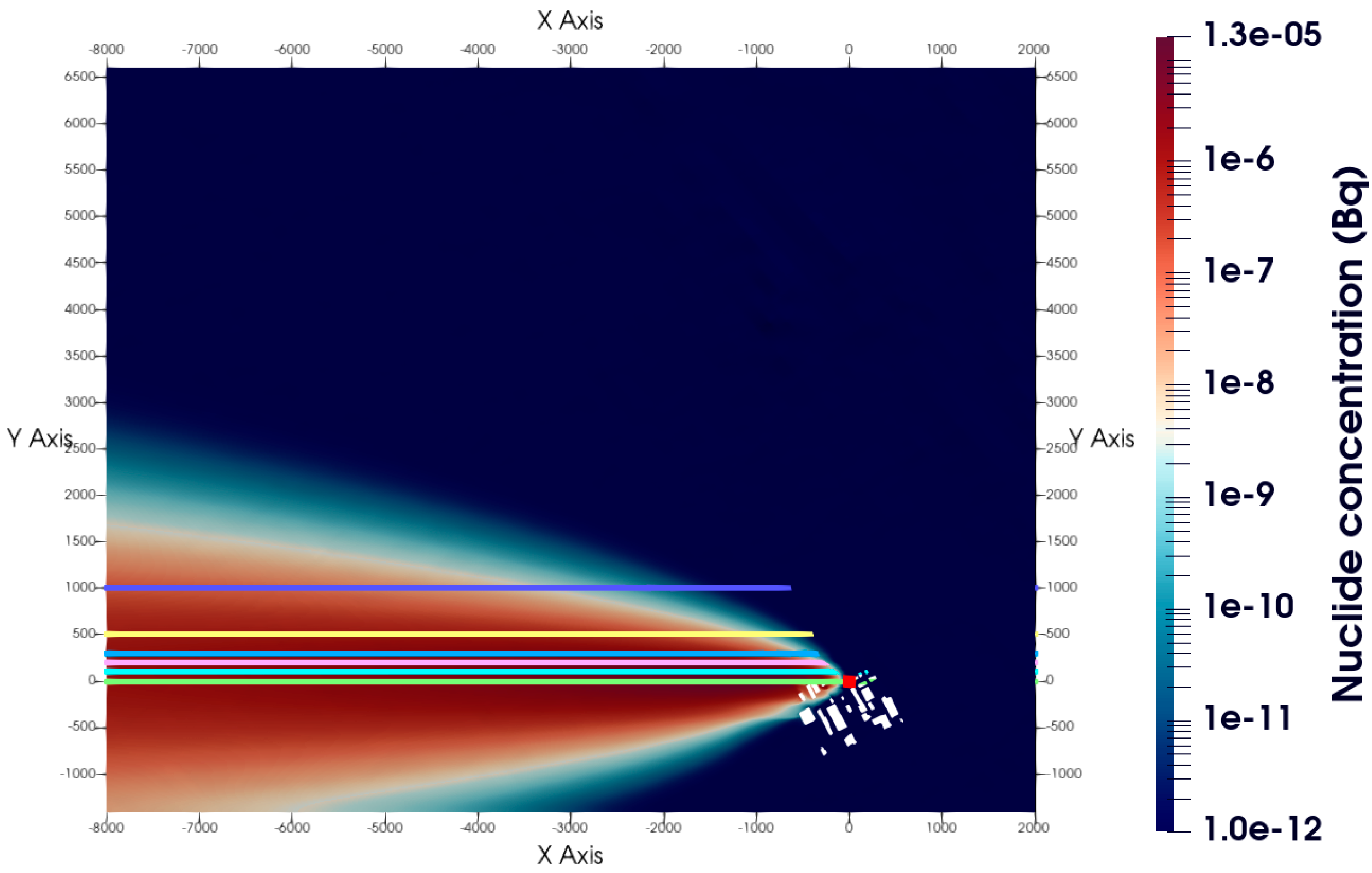
Through data processing of numerical simulation results under two wind speed conditions, Figure 23 and Figure 24 are obtained. Figure 23 illustrates the sampling position distribution of four nuclides (³$H$, ¹⁴$C$, ⁸⁵$Kr$ and ¹²⁹$I$) along six downwind distances from the central release point, represented by green, light blue, magenta, tan, yellow, and purple colors corresponding to 0 m, 100 m, 200 m, 300 m, 500 m, and 1000 m, respectively. The dark red point at the building center indicates the chimney release location.

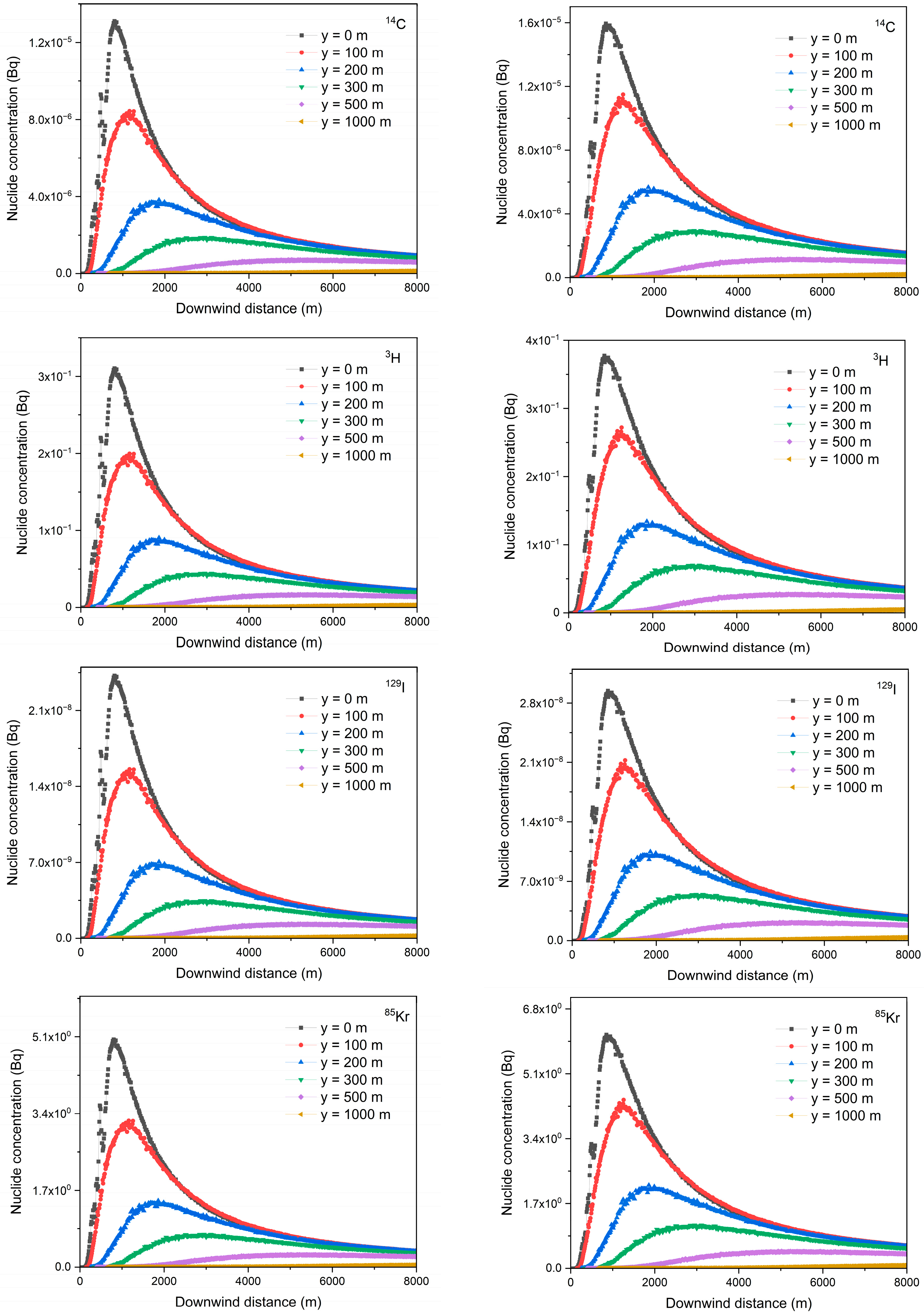
Figure 24 displays the concentration distributions of four nuclides versus distance from the release point, with left and right columns representing higher and lower wind speeds, respectively. Results clearly show that ⁸⁵$Kr$ exhibits the highest concentration among the four nuclides, reaching approximately 6 Bq. This is followed by ³$H$ with a maximum concentration near 0.4 Bq, then ¹⁴$C$ peaking at 1.6 × 10⁻⁵ Bq, and finally ¹²⁹$I$ with a maximum concentration of about 2.8 × 10⁻⁸ Bq. All nuclides demonstrate a rapid concentration increase from 0 m to maximum values at 1000 m downwind, followed by gradual attenuation with increasing distance.

The most significant concentration reduction occurs between 0–100 m and 100–200 m downwind segments. By 500 m and 1000 m distances, the concentration magnitudes decrease by at least one order of magnitude compared to values observed at the downwind center. Notably, data fluctuations along the downwind centerline (y = 0 m) within 1000 m arise from building obstructions that disrupt uniform concentration distribution. Lower wind speeds consistently yield slightly higher nuclide concentrations than higher wind speeds, as reduced airflow diminishes pollutant dispersion capacity, thereby exacerbating environmental contamination and human health risks.

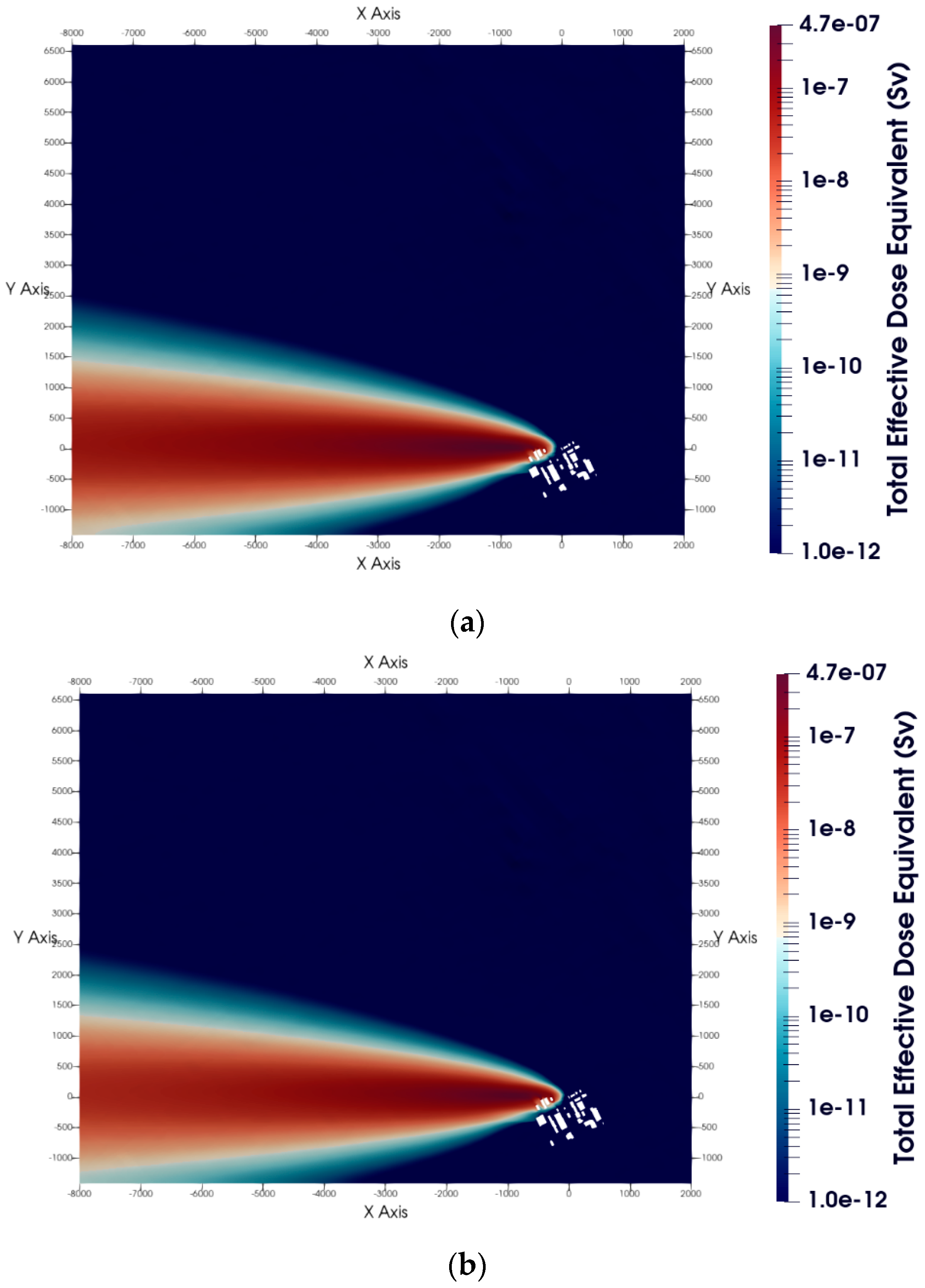
Figure 25 illustrates the Total Effective Dose Equivalent distribution under lower wind speed (a), higher wind speed (b), and their differential distribution (c). While the TEDE patterns in panels a and b appear superficially similar, quantitative analysis reveals significant disparities in the 1000–2000 m downwind range, where TEDE differences reach approximately 1 × 10⁻⁷ Sv—equivalent to 25–33% of the maximum observed values. This highlights the substantial influence of wind speed on pollutant dispersion. However, minimal differences (<5%) are observed near buildings, with discernible contrasts emerging only beyond nuclear facility boundaries.

For both wind speed scenarios, TEDE values remain within the range of 0–4.7 × 10⁻⁷ Sv. These levels fall well below the IAEA public exposure limit of 1 mSv/year and occupational limit of 20 mSv/year, confirming that routine radionuclide emissions from the facility pose no regulatory-compliant health risks. Nevertheless, sustained environmental monitoring of nuclide concentrations is imperative to ensure early detection of potential anomalies.

6. Conclusions

Accurately simulating pollutant dispersion over uneven terrains is a highly challenging and intricate scientific and technological issue that demands resolution. This research centers on the impacts of diverse ABL inlet boundary conditions, turbulent models, and turbulent Schmidt numbers on pollutant dispersion across uneven terrains.

Initially, atmospheric dispersion tracing experiments were carried out in the vicinity of a nuclear facility to acquire the tracer gas concentration at sampling points. Subsequently, improvements were put forward for the default ABL inlet boundary conditions, taking into account the uneven terrain. By leveraging custom boundary conditions in OpenFOAM, an improved ABL inlet condition tailored to uneven terrains was developed. Numerical simulations of pollutant dispersion were executed using two turbulent models, namely the realizable $k-ϵ$ and $SSTk-\omega$, under both default and improved ABL inlet boundary conditions.

The following conclusions were drawn:

(1) Numerical simulations comparing two turbulence models with improved and default ABL inlet boundary conditions indicated that the combination of the $SSTk-\omega$ model and the improved ABL inlet boundary conditions yielded the most satisfactory results when contrasted with the atmospheric dispersion tracer experiment.

(2) In comparison to the improved ABL inlet boundary conditions, the default ABL inlet boundary conditions inaccurately gauged the relative height difference between the cell centers at the inlet boundary and the ground surface. This resulted in larger errors in the near-ground data. As the elevation of the inlet boundary ground surface increased, the disparity between the default and improved ABL boundary conditions became more pronounced, reaching a maximum difference of up to 6 m/s in this study.

(3) Owing to the differences between the improved and default ABL inlet boundary conditions, the distributions of velocity, turbulent kinetic energy, and concentration around the nuclear facility were significantly affected in numerical simulations. The average wind speed difference between buildings was approximately 2 m/s, with a maximum difference reaching up to 4.1 m/s. Regarding turbulent kinetic energy, the majority of the differences were around 0.5, with a maximum difference of up to 1.0. The most substantial impact was on the concentration distribution. Downwind of the chimney, peak ground level pollutant concentrations reached up to 470 times the background level, and a large area had concentrations between 100 and 200 times the background.

(4) Computational fluid dynamics simulations employing dual wind speed regimes (elevated: 4.21 m/s; baseline: 2.5 m/s) were conducted for four characteristic radionuclides. The spatial distribution analysis revealed maximum airborne concentrations at 1000 m downwind for all species, with TEDE (Total Effective Dose Equivalent) profiles demonstrating exponential attenuation patterns in near-surface zones. Comparative evaluation of atmospheric dispersion outcomes showed dose differentials between wind scenarios constituting 33.3% of baseline values (ΔTEDE = 0.47 μSv/yr), yet both remained two orders of magnitude below the IAEA public exposure limit (1 mSv/yr).

References

1. Farrell, J. Fukushima Nuclear Disaster: Lethal Levels of Radiation Detected in Leak Seven Years After Plant Meltdown in Japan. Available online: https://www.independent.co.uk/news/world/asia/fukushima-nuclear-disaster-radiation-lethal-levels-leak-japan-tsunami-tokyo-electric-power-company-a8190981.html (accessed on 19 April 2024).
2. Liu, L.; Guo, H.; Dai, L.; Liu, M.; Xiao, Y.; Cong, T.; Gu, H. The Role of Nuclear Energy in the Carbon Neutrality Goal. Prog. Nucl. Energy 2023, 162, 104772. [Google Scholar] [CrossRef]
3. Zheng, S.; Liu, H.; Guan, W.; Li, B.; Ullah, S. How Do Nuclear Energy and Stringent Environmental Policies Contribute to Achieving Sustainable Development Targets? Nucl. Eng. Technol. 2024, 56, 3983–3992. [Google Scholar] [CrossRef]
4. Pan, X.; Shao, T.; Zheng, X.; Zhang, Y.; Ma, X.; Zhang, Q. Energy and Sustainable Development Nexus: A Review. Energy Strategy Rev. 2023, 47, 101078. [Google Scholar] [CrossRef]
5. Yang, R.; Guo, Q.; Lu, Z. Sensitivity Analysis of Meteorological Parameters to the Airborne Radioactive Materials Diffusion under Normal Operation. Prog. Nucl. Energy 2022, 154, 104479. [Google Scholar] [CrossRef]
6. Hu, T.; Yoshie, R. Effect of Atmospheric Stability on Air Pollutant Concentration and Its Generalization for Real and Idealized Urban Block Models Based on Field Observation Data and Wind Tunnel Experiments. J. Wind Eng. Ind. Aerodyn. 2020, 207, 104380. [Google Scholar] [CrossRef]
7. Ding, S.; Huang, Y.; Cui, P.; Wu, J.; Li, M.; Liu, D. Impact of Viaduct on Flow Reversion and Pollutant Dispersion in 2D Urban Street Canyon with Different Roof Shapes—Numerical Simulation and Wind Tunnel Experiment. Sci. Total Environ. 2019, 671, 976–991. [Google Scholar] [CrossRef]
8. Huang, Z.-R.; Zhang, Y.-J.; Wen, Y.-B.; Tang, Y.-F.; Liu, C.-W.; Zhao, F.-Y. Synoptic Wind Driven Ventilation and Far Field Radionuclides Dispersion across Urban Block Regions: Effects of Street Aspect Ratios and Building Array Skylines. Sustain. Cities Soc. 2022, 78, 103606. [Google Scholar] [CrossRef]
9. Guo, D.; Yang, F.; Shi, X.; Li, Y.; Yao, R. Numerical Simulation and Wind Tunnel Experiments on the Effect of a Cubic Building on the Flow and Pollutant Diffusion under Stable Stratification. Build. Environ. 2021, 205, 108222. [Google Scholar] [CrossRef]
10. Luo, T.; Yu, C.; Liu, R.; Li, M.; Zhang, J.; Qu, S. Numerical Simulation of LNG Release and Dispersion Using a Multiphase CFD Model. J. Loss Prev. Process Ind. 2018, 56, 316–327. [Google Scholar] [CrossRef]
11. An, J.; Xiang, W.; Han, Z.; Xiao, K.; Wang, Z.; Wang, X.; Wu, J.; Yan, P.; Li, J.; Chen, Y.; et al. Validation of the Institute of Atmospheric Physics Emergency Response Model with the Meteorological Towers Measurements and SF6 Diffusion and Pool Fire Experiments. Atmos. Environ. 2013, 81, 60–67. [Google Scholar] [CrossRef]
12. Guo, D.; Zhao, P.; Wang, R.; Yao, R.; Hu, J. Numerical Simulations of the Flow Field and Pollutant Dispersion in an Idealized Urban Area under Different Atmospheric Stability Conditions. Process Saf. Environ. Prot. 2020, 136, 310–323. [Google Scholar] [CrossRef]
13. Xie, Z.T. Modelling Street-Scale Flow and Dispersion in Realistic Winds-Towards Coupling with Mesoscale Meteorological Models. Bound. Layer Meteorol. 2011, 141, 53–75. [Google Scholar] [CrossRef]
14. Liu, J.; Tan, L.; Ma, Y. An Integrated Risk Assessment Method for Urban Areas Due to Chemical Leakage Accidents. Reliab. Eng. Syst. Saf. 2024, 247, 110091. [Google Scholar] [CrossRef]
15. Wang, S.; Zheng, X.; Wang, J.; Yang, J. Numerical Study on the Gaseous Radioactive Pollutant Dispersion in Urban Area from the Upstream Wind: Impact of the Urban Morphology. Nucl. Eng. Technol. 2024, 56, 2039–2049. [Google Scholar] [CrossRef]
16. Wu, N.; Xue, N.; Liu, X. Research on the Influence of Complex Terrain on Atmospheric Dispersion After Accident. In Proceedings of the International Conference on Nuclear Engineering, London, UK, 22–26 July 2018. [Google Scholar]
17. Kocijan, J.; Hvala, N.; Perne, M.; Mlakar, P.; Grašič, B.; Božnar, M.Z. Surrogate Modelling for the Forecast of Seveso-Type Atmospheric Pollutant Dispersion. Stoch. Environ. Res. Risk Assess. 2023, 37, 275–290. [Google Scholar] [CrossRef]
18. Hoq, M.A.; Soner, M.A.M.; Khanom, S.; Uddin, M.J.; Moniruzzaman, M.; Chowdhury, M.S.H.; Helal, A.; Khaer, M.A.; Hassan, S.M.T.; Chowdhury, M.T.; et al. Assessment of Radiation Dose Associated with the Atmospheric Release of 41Ar from the TRIGA Mark-II Research Reactor in Bangladesh. Sci. Technol. Nucl. Install. 2024, 2024, 9141535. [Google Scholar] [CrossRef]
19. Guo, D.; Wang, J.; Ge, D.; Chen, C.; Chen, L. Oceanic Radionuclide Dispersion Method Investigation for Nonfixed Source from Marine Reactor Accident. Sci. Technol. Nucl. Install. 2022, 2022, 2822857. [Google Scholar] [CrossRef]
20. Clements, D.; Coburn, M.; Cox, S.J.; Bulot, F.M.J.; Xie, Z.T.; Vanderwel, C. Comparing Large-Eddy Simulation and Gaussian Plume Model to Sensor Measurements of an Urban Smoke Plume. Atmosphere 2024, 15, 1089. [Google Scholar] [CrossRef]
21. Xing, J.; Liu, Z.; Huang, P.; Feng, C.; Zhou, Y.; Zhang, D.; Wang, F. Experimental and Numerical Study of the Dispersion of Carbon Dioxide Plume. J. Hazard. Mater. 2013, 256, 40–48. [Google Scholar] [CrossRef] [PubMed]
22. Ricci, A.; Kalkman, I.; Blocken, B.; Burlando, M.; Repetto, M.P. Impact of Turbulence Models and Roughness Height in 3D Steady RANS Simulations of Wind Flow in an Urban Environment. Build. Environ. 2020, 171, 106617. [Google Scholar] [CrossRef]
23. Pope, S.B. Turbulent Flows; Cambridge University Press: Cambridge, UK, 2000; ISBN 9780521598866. [Google Scholar]
24. Blocken, B. Computational Fluid Dynamics for Urban Physics: Importance, Scales, Possibilities, Limitations and Ten Tips and Tricks towards Accurate and Reliable Simulations. Build. Environ. 2015, 91, 219–245. [Google Scholar] [CrossRef]
25. Deardorff, J.W. A Numerical Study of Three-Dimensional Turbulent Channel Flow at Large Reynolds Numbers. J. Fluid Mech. 1970, 41, 453–480. [Google Scholar] [CrossRef]
26. Xie, Z.-T.; Castro, I.P. Efficient Generation of Inflow Conditions for Large Eddy Simulation of Street-Scale Flows. Flow Turbul. Combust. 2008, 81, 449–470. [Google Scholar] [CrossRef]
27. Stoll, R.; Gibbs, J.A.; Salesky, S.T.; Anderson, W.; Calaf, M.; Stoll, R.; Gibbs, J.A.; Salesky, S.T.; Anderson, W.; Calaf, M. Review: Large-Eddy Simulation of the Atmospheric Boundary Layer. Bound. Layer Meteorol. 2020, 177, 541–581. [Google Scholar] [CrossRef]
28. Blocken, B. LES over RANS in Building Simulation for Outdoor and Indoor Applications: A Foregone Conclusion? Build. Simul. 2018, 11, 821–870. [Google Scholar] [CrossRef]
29. Xing, L.; Zhang, J.; Zhang, M.; Li, Y.; Zhang, S.; Yan, T. A Reasonable Inlet Boundary for Wind Simulation Based on a Trivariate Joint Distribution Model. J. Wind Eng. Ind. Aerodyn. 2023, 233, 105325. [Google Scholar] [CrossRef]
30. Liang, Q.; Miao, Y.; Zhang, G.; Liu, S. Simulating Microscale Urban Airflow and Pollutant Distributions Based on Computational Fluid Dynamics Model: A Review. Toxics 2023, 11, 927. [Google Scholar] [CrossRef]
31. Liu, Y.; Cao, H.; Zhao, P.; Yang, G.; Yu, H.; He, F.; He, B. Study on Flow Field Simulation at Transmission Towers in Loess Hilly Regions Based on Circular Boundary Constraints. Energy Eng. J. Assoc. Energy Eng. 2023, 120, 2417–2431. [Google Scholar] [CrossRef]
32. Han, Y.; Stoellinger, M.K. RANS Simulations of Neutral Atmospheric Boundary Layer Flow over Complex Terrain with Comparisons to Field Measurements. Wind Energy 2020, 23, 91–119. [Google Scholar] [CrossRef]
33. Che, Y.; Salazar, A.A.; Peng, S.; Zheng, J.; Chen, Y.; Yuan, L. A Multi-Scale Model for Day-Ahead Wind Speed Forecasting: A Case Study of the Houhoku Wind Farm, Japan. Sustain. Energy Technol. Assess. 2022, 52, 101995. [Google Scholar] [CrossRef]
34. Jia, R.; Yang, J.; Zhu, X.; Xu, F.; Wang, L. A Study on the Gaseous Radionuclide Dispersion in the Highway across Urban Blocks: Effects of the Urban Morphology, Roadside Vegetation and Leakage Location. Sustain. Cities Soc. 2023, 95, 104617. [Google Scholar] [CrossRef]
35. Xin, B.; Dang, W.; Yan, X.; Yu, J.; Bai, Y. Dispersion Characteristics and Hazard Area Prediction of Mixed Natural Gas Based on Wind Tunnel Experiments and Risk Theory. Process Saf. Environ. Prot. 2021, 152, 278–290. [Google Scholar] [CrossRef]
36. Jiang, X.; Yang, H.; Lin, G.; Dang, W.; Yu, A.; Zhang, J.; Gu, M.; Ge, C. Measurements and Predictions of Harmful Releases of the Gathering Station over the Mountainous Terrain. J. Loss Prev. Process Ind. 2021, 71, 104485. [Google Scholar] [CrossRef]
37. Yuan, S.; Cai, J.; Reniers, G.; Yang, M.; Chen, C.; Wu, J. Safety Barrier Performance Assessment by Integrating Computational Fluid Dynamics and Evacuation Modeling for Toxic Gas Leakage Scenarios. Reliab. Eng. Syst. Saf. 2022, 226, 108719. [Google Scholar] [CrossRef]
38. Coburn, M.; Vanderwel, C.; Herring, S.; Xie, Z.T. Impact of Local Terrain Features on Urban Airflow. Bound. Layer Meteorol. 2023, 189, 189–213. [Google Scholar] [CrossRef]
39. Lin, C.; Ooka, R.; Kikumoto, H.; Sato, T.; Arai, M. CFD Simulations on High-Buoyancy Gas Dispersion in the Wake of an Isolated Cubic Building Using Steady RANS Model and LES. Build. Environ. 2021, 188, 107478. [Google Scholar] [CrossRef]
40. Lin, C.; Ooka, R.; Kikumoto, H.; Jia, H. Eulerian RANS Simulations of Near-Field Pollutant Dispersion around Buildings Using Concentration Diffusivity Limiter with Travel Time. Build. Environ. 2021, 202, 108047. [Google Scholar] [CrossRef]
41. Zhao, R.; Liu, S.; Liu, J.; Jiang, N.; Chen, Q. Generalizability Evaluation of K-ε Models Calibrated by Using Ensemble Kalman Filtering for Urban Airflow and Airborne Contaminant Dispersion. Build. Environ. 2022, 212, 108823. [Google Scholar] [CrossRef]
42. Roetzer, H.; Riesing, J. Measurement of the Contribution of a Single Plant to Air Pollution Using the SF6-Tracer Technique; WIT Press: Southampton, UK, 1996; Volume 8. [Google Scholar]
43. Martin, D.; Petersson, K.F.; Shallcross, D.E. The Use of Cyclic Perfluoroalkanes and SF 6 in Atmospheric Dispersion Experiments. Q. J. R. Meteorol. Soc. 2011, 137, 2047–2063. [Google Scholar] [CrossRef]
44. Flaherty, J.E. Investigation of Atmospheric Dispersion in an Urban Environment Using SF 6 Tracer and Numerical Methods. Ph.D. Thesis, Washington State University, Pullman, WA, USA, 2005. [Google Scholar]
45. Connan, O.; Leroy, C.; Derkx, F.; Maro, D.; Hébert, D.; Roupsard, P.; Rozet, M. Atmospheric Dispersion of an Elevated Release in a Rural Environment: Comparison between Field SF6 Tracer Measurements and Computations of Briggs and ADMS Models. Atmos. Environ. 2011, 45, 7174–7183. [Google Scholar] [CrossRef]
46. Diaz, A.P.; Gryning, S.E.; Hasager, C.B.; Courtney, M. General Rights Extending the Wind Profile Much Higher than the Surface Layer. In Proceedings of the 2009 European Wind Energy Conference and Exhibition, Marseille, France, 16–19 March 2009. [Google Scholar]
47. Hu, P.; Li, Y.; Cai, C.S.; Liao, H.; Xu, G.J. Numerical Simulation of the Neutral Equilibrium Atmospheric Boundary Layer Using the SST K-ω Turbulence Model. Wind Struct. Int. J. 2013, 17, 87–105. [Google Scholar] [CrossRef]
48. Hu, P.; Li, Y.; Han, Y.; Cai, S.C.S.; Xu, X. Numerical Simulations of the Mean Wind Speeds and Turbulence Intensities over Simplified Gorges Using the SST K-ω Turbulence Model. Eng. Appl. Comput. Fluid Mech. 2016, 10, 359–372. [Google Scholar] [CrossRef]
49. OpenFOAM OpenFOAM: User Guide V2012 the Open Source CFD Toolbox. Available online: https://www.openfoam.com/documentation/guides/v2012/doc/guide-bcs-inlet-atm-atmBoundaryLayer.html (accessed on 14 October 2025).
50. Shih, T.H.; Liou, W.; Shabbir, A.; Yang, Z.; Zhu, J. A New K-ϵ Eddy Viscosity Model for High Reynolds Number Turbulent Flows. Comput. Fluids 1994, 24, 227–238. [Google Scholar] [CrossRef]
51. Gromke, C.; Blocken, B. Influence of Avenue-Trees on Air Quality at the Urban Neighborhood Scale. Part I: Quality Assurance Studies and Turbulent Schmidt Number Analysis for RANS CFD Simulations. Environ. Pollut. 2015, 196, 214–223. [Google Scholar] [CrossRef] [PubMed]
52. Mittal, H.; Sharma, A.; Gairola, A. A Review on the Study of Urban Wind at the Pedestrian Level around Buildings. J. Build. Eng. 2018, 18, 154–163. [Google Scholar] [CrossRef]
53. van Druenen, T.; van Hooff, T.; Montazeri, H.; Blocken, B. CFD Evaluation of Building Geometry Modifications to Reduce Pedestrian-Level Wind Speed. Build. Environ. 2019, 163, 106293. [Google Scholar] [CrossRef]
54. Shirzadi, M.; Tominaga, Y. Multi-Fidelity Shape Optimization Methodology for Pedestrian-Level Wind Environment. Build. Environ. 2021, 204, 108076. [Google Scholar] [CrossRef]
55. Yang, A.-S.; Su, Y.-M.; Wen, C.-Y.; Juan, Y.-H.; Wang, W.-S.; Cheng, C.-H. Estimation of Wind Power Generation in Dense Urban Area. Appl. Energy 2016, 171, 213–230. [Google Scholar] [CrossRef]
56. Tominaga, Y.; Stathopoulos, T. Turbulent Schmidt Numbers for CFD Analysis with Various Types of Flowfield. Atmos. Environ. 2007, 41, 8091–8099. [Google Scholar] [CrossRef]
57. Hanna, S.R.; Strimaitis, D.G.; Scire, J.S.; Moore, G.E.; Kessler, R.C. Overview of Results of Analysis of Data from the South-Central Coast Cooperative Aerometric Monitoring Program (SCCCAMP 1985). J. Appl. Meteorol. Climatol. 1991, 30, 511–533. [Google Scholar] [CrossRef]
58. Hanna, S.R.; Chang, J.C.; Strimaitis, D.G. Hazardous Gas Model Evaluation with Field Observations. Atmos. Environ. Part A Gen. Top. 1993, 27, 2265–2285. [Google Scholar] [CrossRef]
59. Hanna, S.R. Air Quality Model Evaluation and Uncertainty. JAPCA 1988, 38, 406–412. [Google Scholar] [CrossRef]
60. Hanna, S.R. Uncertainties in Air Quality Model Predictions. Bound. Layer Meteorol. 1993, 62, 3–20. [Google Scholar] [CrossRef]
61. Hanna, S. Confidence Limits for Air Quality Model Evaluations as Estimated by Bootstrap and Jackknife Resampling Methods. Atmos. Environ. 1989, 23, 1385–1398. [Google Scholar] [CrossRef]
62. Bellamy, M.B.; Dewji, S.A.; Leggett, R.W.; Hiller, M.; Veinot, K.; Manger, R.P.; Eckerman, K.F.; Ryman, J.C.; Easterly, C.E.; Hertel, N.E.; et al. External Exposure to Radionuclides in Air, Water, and Soil; USA Environmental Protection Agency: Washington, DC, USA, 2019.
63. Ma, J.; Ma, J.L.; Li, R. Environmental Assessment and Analysis on the Siting Stage of Spent Nuclear Fuel Reprocessing Plant. Nucl. Sci. Eng. 2015, 35, 333–338. [Google Scholar]
64. USGS Shuttle Radar Topography Mission (SRTM) Database. Available online: https://lta.cr.usgs.gov/SRTM (accessed on 28 March 2024).
65. Franke, J.; Hellsten, A.; Schlünzen, H.; Carissimo, B. The COST 732 Best Practice Guideline for CFD Simulation of Flows in the Urban Environment: A Summary. Int. J. Environ. Pollut. 2011, 44, 419–427. [Google Scholar] [CrossRef]
66. Tominaga, Y.; Mochida, A.; Yoshie, R.; Kataoka, H.; Nozu, T.; Yoshikawa, M.; Shirasawa, T. AIJ Guidelines for Practical Applications of CFD to Pedestrian Wind Environment around Buildings. J. Wind Eng. Ind. Aerodyn. 2008, 96, 1749–1761. [Google Scholar] [CrossRef]
67. Franke, J. Recommendations of the COST Action C14 on the Use of CFD in Predicting Pedestrian Wind Environment. In Proceedings of the Fourth International Symposium on Computational Wind Engineering, Yokohama, Japan, 16–19 July 2006; pp. 529–532. [Google Scholar]
68. Abu-Zidan, Y.; Mendis, P.; Gunawardena, T. Optimising the Computational Domain Size in CFD Simulations of Tall Buildings. Heliyon 2021, 7, e06723. [Google Scholar] [CrossRef] [PubMed]
69. Weller, H.G.; Tabor, G.; Jasak, H.; Fureby, C. A Tensorial Approach to Computational Continuum Mechanics Using Object-Oriented Techniques. Comput. Phys. 1998, 12, 620–631. [Google Scholar] [CrossRef]
70. Guibas, L.; Stolfi, J. Primitives for the Manipulation of General Subdivisions and the Computation of Voronoi. ACM Trans. Graph. 1985, 4, 74–123. [Google Scholar] [CrossRef]
71. Lee, D.T.; Schachter, B.J. Two Algorithms for Constructing a Delaunay Triangulation. Int. J. Comput. Inf. Sci. 1980, 9, 219–242. [Google Scholar] [CrossRef]
72. Lawson, C.L. Software for c1 surface interpolation. In Mathematical Software; John, R.R., Ed.; Academic Press: Cambridge, MA, USA, 1977; pp. 161–194. ISBN 978-0-12-587260-7. [Google Scholar] [CrossRef]
73. Surfer Help Triangulation with Linear Interpolation. Available online: https://surferhelp.goldensoftware.com/griddata/idd_grid_data_triangulation.htm (accessed on 7 April 2024).
Figure 1. The location of the nuclear facilities and their surrounding geographical environment, the boundary of the physical model, the sampling point of the atmospheric diffusion tracer experiment, the release point, weather station and the wind direction information.
Atmosphere 16 01203 g001
Figure 2. Time series of tower observations during the tracer experiment: (a) air temperature at 10, 30, 50, 70 and 100 m; (b) wind speed at the same heights; (c) wind direction; and (d) estimated Monin–Obukhov length L.
Atmosphere 16 01203 g002
Figure 3. Development of a framework for calculating the inlet boundary conditions of the atmospheric boundary layer over complex terrain. Validation and evaluation of numerical simulation results and atmospheric dispersion tracer experiments through comparisons with improved versus default ABL inlet boundary conditions, various turbulence models, and different turbulent Schmidt numbers.
Atmosphere 16 01203 g003
Figure 4. Schematic diagram of the steps for improved atmospheric boundary layer inlet boundary conditions.
Atmosphere 16 01203 g004
Figure 5. Overview of calculation range of nuclear facilities and their surrounding environment.
Atmosphere 16 01203 g005
Figure 6. Wind speed profiles measured on the y = 0 plane at (a) x = 0 and (b) x = 20 for the Basic, Medium, Fine, and Extra Fine grids. Turbulent kinetic energy k profiles measured on the y = 0 plane at (c) x = 0 and (d) x = 20 for the Basic, Medium, Fine, and Extra Fine grids.
Atmosphere 16 01203 g006
Figure 7. Perspective view of the model geometry and domain. Computational domain with refined meshing near terrain and building geometry. Zoomed in view of the mesh around building geometry with local refinement of a minimum of 1 m. Inflation layers have been added to cover all surfaces in the terrain and buildings.
Atmosphere 16 01203 g007
Figure 8. y+ achieved with the mesh from current work.
Atmosphere 16 01203 g008
Figure 9. Sulfur hexafluoride (SF6) concentration distribution map.
Atmosphere 16 01203 g009
Figure 10. Comparison of velocity field between improved and default atmospheric boundary layer inlet boundary.
Atmosphere 16 01203 g010
Figure 11. Scatter plot of predicted and measured maximum SF6 concentration. The black dashed line indicates that the predicted value is equal to the observed value, the red solid line indicates twice the observed value, and the purple broken point.
Atmosphere 16 01203 g011
Figure 12. Fractional bias (FB) and normalized mean square error (NMSE) for SF6 concentrations under predicted and measured conditions. The purple and blue dash-dot lines indicate the acceptable ranges for FB (−0.3 < FB < 0.3) and NMSE (<4.0), while the black parabola represents the minimum NMSE for a given FB (NMSE = 4FB2/(4 − FB2)). The red line indicates the unbiased condition (FB = 0).
Atmosphere 16 01203 g012
Figure 13. Plot of geometric mean (MG) versus geometric variance (VG) for SF6 concentration for the two models with improved and default ABL, the RKE and SST models. The solid black parabola represents the minimum VG for a given MG (VG = (MG − 1)2 + 1).
Atmosphere 16 01203 g013
Figure 14. Improved and default models are four different distances at high and low altitude inlet conditions. Red and blue terrain indicate that the altitude is above 1300 m and below.
Atmosphere 16 01203 g014
Figure 15. Velocity profile diagrams at two inlet positions, x = 0 m and x = 3000 m, as well as the diagram of percentage differences between the improved and default inlet boundary conditions. Percent = (Udefault − Uimproved)/Udefault × 100%.
Atmosphere 16 01203 g015
Figure 16. Comparison of velocity profiles between the improved and default atmospheric boundary layer inlet boundary conditions. The solid line represents the improved ABL, and the dotted line represents the default ABL. (a) Low-altitude inlet conditions; (b) high-altitude inlet conditions.
Atmosphere 16 01203 g016
Figure 17. Comparison of turbulent kinetic energy profiles between the improved and default atmospheric boundary layer inlet boundary conditions. The solid line represents the improved ABL, and the dotted line represents the default ABL. (a) Low-altitude inlet conditions; (b) high-altitude inlet conditions.
Atmosphere 16 01203 g017
Figure 18. Validation of mean velocities from simulations of four conditions at the measurement locations shown in Figure 8.
Atmosphere 16 01203 g018
Figure 19. Velocity magnitude comparison and the absolute velocity magnitude difference between the default and improved ABL cases at height of Z = 1270 m. The difference is calculated as Udiff = |mag(Udefault) − mag(Uimproved)|.
Atmosphere 16 01203 g019
Figure 20. Turbulent kinetic energy and its absolute difference contour between the default and improved ABL cases at height of Z = 1270 m. The difference is calculated as kdiff = |kdefault − kimproved)|.
Atmosphere 16 01203 g020
Figure 21. Normalized tracer-gas concentration (C/C0) and its absolute difference contour between the default and improved ABL cases at height of Z = 1270 m. The difference is calculated as Cdiff = |Cdefault − Cimproved)|/C0.
Atmosphere 16 01203 g021
Figure 22. Comprehensive evaluation index of different Schmidt numbers.
Atmosphere 16 01203 g022
Figure 23. Regarding the distribution of nuclide 14 C on the ground surface and the six monitoring lines for pollutant distribution.
Atmosphere 16 01203 g023
Figure 24. The distribution patterns of four nuclides (3 H , 14 C , 85 K r , 129 I ) within an 8 km downwind range under both higher and lower wind speed conditions.
Atmosphere 16 01203 g024
Figure 25. Distribution patterns and differential maps of total effective dose equivalent under lower and higher wind speed conditions. The figure illustrates the TEDE distribution under (a) lower wind speed, (b) higher wind speed, and (c) their differential distribution.
Atmosphere 16 01203 g025aAtmosphere 16 01203 g025b