Joint Modeling of Pixel-Wise Visibility and Fog Structure for Real-World Scene Understanding

Abstract

Reduced visibility caused by foggy weather has a significant impact on transportation systems and driving safety, leading to increased accident risks and decreased operational efficiency. Traditional methods rely on expensive physical instruments, limiting their scalability. To address this challenge in a cost-effective manner, we propose a two-stage network for visibility estimation from stereo image inputs. The first stage computes scene depth via stereo matching, while the second stage fuses depth and texture information to estimate metric-scale visibility. Our method produces pixel-wise visibility maps through a physically constrained, progressive supervision strategy, providing rich spatial visibility distributions beyond a single global value. Moreover, it enables the detection of patchy fog, allowing a more comprehensive understanding of complex atmospheric conditions. To facilitate training and evaluation, we propose an automatic fog-aware data generation pipeline that incorporates both synthetically rendered foggy images and real-world captures. Furthermore, we construct a large-scale dataset encompassing diverse scenarios. Extensive experiments demonstrate that our method achieves state-of-the-art performance in both visibility estimation and patchy fog detection.

1. Introduction

Visibility refers to the maximum distance at which a target object can be clearly seen by the human eye under specific atmospheric conditions. According to the definition provided by the International Civil Aviation Organization (ICAO), this concept specifically refers to the visibility of a black object of suitable size against a uniform sky background during daylight or moonless nights. In foggy conditions, airborne water droplets scatter light, reducing the contrast and brightness of distant objects and thus degrading visibility. Similarly, haze and particulate matter also degrade visual clarity through both absorption and scattering effects.

Haze and fog significantly impact the transportation industry by reducing visibility. Under such conditions, the risk of traffic accidents increases substantially. In particular, on highways, airport runways, and during maritime navigation, drivers and operators often struggle to perceive obstacles or road conditions ahead, leading to a heightened risk of severe collisions [1]. The Federal Highway Administration (FHWA) estimated that more than 38,700 road accidents occur each year due to foggy conditions. Over 16,300 people are injured in foggy weather incidents every year, with more than 600 fatalities occurring each year [2]. Statistical data indicate that the number of accidents caused by fog each year constitutes a considerable proportion of all accidents, posing serious challenges to public safety.

In this context, accurate visibility estimation becomes particularly crucial. It enables authorities to issue timely warnings and take preventive actions to reduce the risk of accidents. For instance, in the aviation industry, airlines can adjust flight schedules based on the latest visibility predictions to ensure flight safety. Traffic management authorities, on the other hand, can utilize real-time data to modify speed limits or implement temporary road closures, thus preventing traffic accidents [3]. In addition to enhancing safety, accurate visibility estimation also contributes to improving the overall efficiency of transportation systems [4]. For instance, in logistics and freight delivery, knowledge of visibility conditions enables more effective route planning, allowing vehicles to avoid areas with reduced visibility and enhancing delivery speed. Similarly, ports and airports can also leverage visibility forecasts to optimize scheduling and operations, ensuring smooth operations under favorable conditions [5].

Given the aforementioned importance, researchers have continuously explored new approaches to improve the accuracy of visibility estimation in recent years [6]. Early methods primarily relied on statistical analysis, estimating visibility by investigating the relationships between image features and visibility levels—for example, techniques based on the dark channel prior [7,8,9,10,11]. With advances in computer vision and deep learning technologies, models based on convolution neural network (CNN) [12,13,14,15,16,17,18,19,20] and transformer block [21,22,23] have gradually become dominant. These methods are capable of extracting complex features from input images and learning intricate relationships between these features and visibility levels, thereby achieving more accurate and robust estimation results.

However, most existing methods rely solely on monocular RGB image as input, lacking access to accurate scene geometric information [6]. From the perspective of Koschmieder’s haze model [24], estimating precise visibility values fundamentally requires knowledge of scene depth, which is inherently missing in monocular setups. Current monocular approaches either estimate only the transmittance map without providing explicit visibility values, or attempt to infer depth through deep learning techniques. However, recovering metric scene depth from a single RGB image is inherently ill-posed, and the resulting depth maps often lack the reliability needed for accurate visibility estimation.

To address this limitation, we propose a two-stage network based on transformer architecture that utilizes binocular RGB images as input. The stereo images provide sufficient and reliable scene scale information, enabling a more robust and accurate visibility estimation process. In the first stage, the network utilizes a recurrent stereo matching network to derive the depth information of the scene. In the second stage, we propose a bidirectional cross-attention block (BCB) to align the RGB texture features with the depth information. After undergoing the feature alignment and the fusion of multi-scale features, the network produces a comprehensive feature map. Finally, a head layer is attached to compute the pixel-wise visibility map.

After obtaining the pixel-wise visibility estimation from the network, we design a mechanism that detects the presence of non-uniform patchy fog by analyzing the spatial distribution differences of the estimated visibility values. This mechanism generates a confidence score indicating the likelihood of uneven fog occurring in the scene. When the confidence score exceeds a predefined threshold, it can be determined that non-uniform patchy fog is present. This detection capability is of significant importance for transportation systems, as patchy fog is a critical factor affecting traffic safety.

To facilitate more effective model training, we propose an automatic pipeline for constructing synthetic foggy images to augment the real-world collections. First, we collect RGB images captured under clear-weather conditions from various sources, including web images, public datasets, Carla simulator [25], and highway or urban traffic cameras. We employ stereo depth estimation models such as Monster [26] to obtain the corresponding scene depth information. Finally, guided by the Koschmieder’s haze model [24], we utilize the estimated depth maps together with the clear-weather RGB images to synthesize foggy images with specified visibility levels. In addition, we introduce Gaussian perturbations during the generation of uniform fog to synthesize patchy fog images. Benefiting from the diversity of the data sources, the proposed pipeline enables the efficient and automatic generation of large-scale foggy image datasets required for training and evaluation.

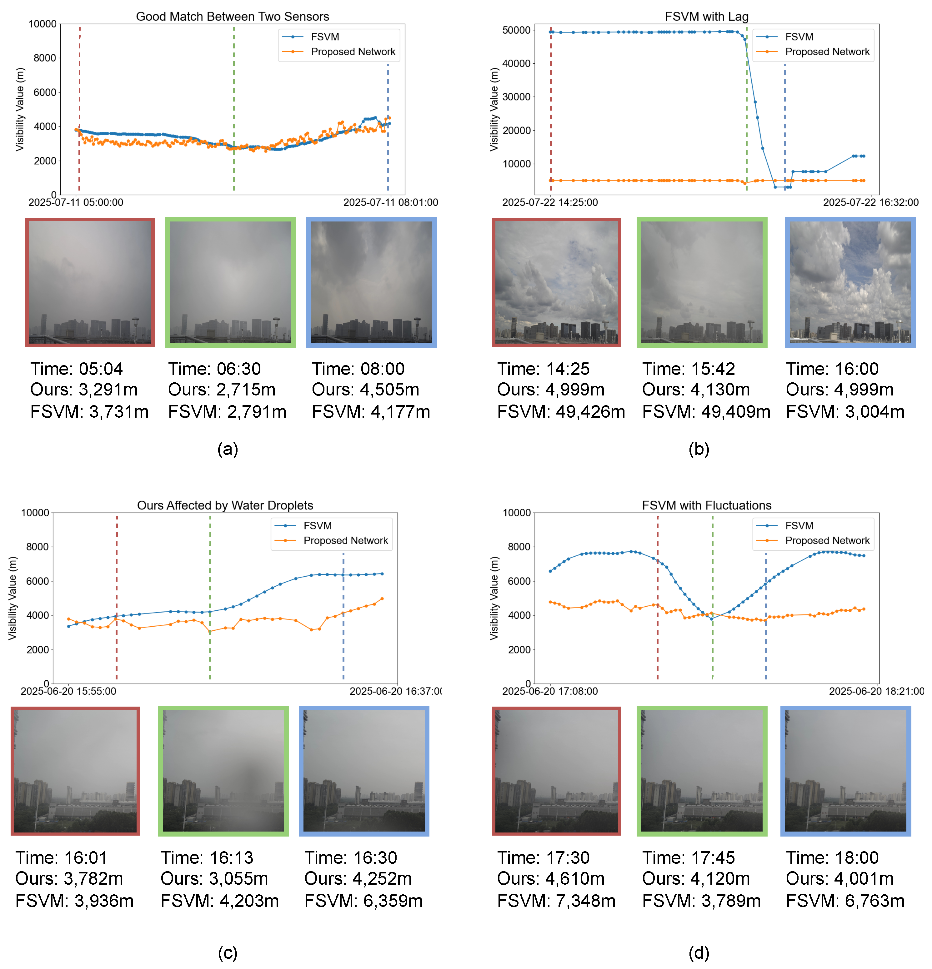
To evaluate the effectiveness of our method, we conduct both comparative and ablation studies on a synthetic fog dataset. Moreover, we build a real-world system equipped with a binocular camera unit and a pan-tilt unit. We compare our estimates against measurements from a forward scatter visibility meter (FSVM) and validate the system using real-world image sequences.

To sum up, our contributions are as follows:

1.

We propose a two-stage network that utilizes stereo image inputs and a physically grounded, progressive training paradigm to achieve accurate pixel-wise visibility estimation of scenes.

2.

We introduce a mechanism for detecting patchy fog by analyzing the spatial variation in visibility results.

3.

We present an automatic technique for generating foggy images and a pipeline for constructing foggy image datasets.

4.

Experimental results on both the dataset and real-world environments demonstrate that our proposed methods can accurately estimate visibility across diverse scenes and detect the presence of fog patches within images.

Our work can be found at https://github.com/HexaWarriorW/Pixel-Wise-Visibility (accessed on 16 September 2025). The remainder of this paper is organized as follows. Section 2 presents the related work in key areas relevant to this study. Section 3 introduces the problem setup investigated in this paper, along with the associated mathematical models. Section 4 describes the construction methodology of the foggy image dataset we built. Section 5 details the architecture of our proposed network and the loss functions used during training. Section 6 covers the experimental setup, including comprehensive experiments and ablation studies conducted on both synthetic datasets and real-world scenarios to evaluate the model’s performance. Finally, Section 7 summarizes the main findings of this work and provides an outlook on potential future research directions.

2. Related Work

2.1. Image-Based Visibility Estimation

In previous studies, image-based visibility estimation methods can be roughly categorized into three groups: traditional algorithms, machine learning approaches, and deep learning methods.

The first category consists of traditional algorithms. Many methods estimate atmospheric light and transmittance by leveraging the dark channel prior (DCP) theory [27], and then convert scene depth into visibility based on the Koschmieder’s haze model [24]. Some approaches estimate visibility directly based on its physical definition by identifying the farthest visible object in the scene as a reference. For instance, Pomerleau [28] detected lane markings from images captured by an onboard camera and subsequently estimated visibility by analyzing the attenuation of contrast along the road. Some other methods establish empirical formulas for visibility estimation by analyzing the statistical relationships between image features and visibility levels.

The second group involves traditional machine learning, for example, L. Yang et al. [29] employed an SVM classifier to rate foggy images into different visibility levels. The proposed methodology integrates two image processing techniques. Specifically, it combines the improved dark channel prior and weighted image entropy with a support vector machine classifier to enable real-time visibility estimation. The third category is based on deep learning methods. As early as 1995, researchers began employing Multi-Layer Perceptron for visibility estimation [30,31]. Since then, with the rise of CNN [12,13,14,15,16,20] in computer vision, CNN-based approaches have been increasingly adopted in this domain. In most of these methods, CNNs are used either to extract discriminative features from input images or to learn the underlying correlations between these features and visibility levels. Some recent approaches also explore the integration of physical laws into the learning framework, aiming to enhance both model interpretability and performance. For instance, DMRVisNet [20] estimates visibility by integrating a physical model into its framework, rather than directly predicting the visibility value using a convolution neural network. Similarly, DQVENet [32] simultaneously performs monocular depth estimation and monocular transmittance map estimation, achieving favorable visibility estimation results in long-range traffic scenarios. In recent years, transformer-based methods [21,22,23] have increasingly been applied in the field of visibility estimation. Fgs-net [23] embeds the coordinate attention module in order to obtain more efficient learned features.

Although the aforementioned methods achieve promising results in visibility estimation, they rely on monocular inputs and lack depth cues, limiting their accuracy and generalization in real-world scenarios. Our approach takes stereo images as input and leverages a carefully designed network architecture and training strategy to jointly enforce semantic and structural consistency. This integration enables more accurate and better-generalized visibility estimation. Furthermore, our method can analyze the distribution of visibility maps to detect the presence of patchy fog.

2.2. Foggy Image Generation

Due to the scarcity of real-world foggy images and the difficulty in acquiring dense visibility ground truth, generating foggy images is crucial for deep learning-based visibility estimation. In such a field, given the known depth information, most existing synthetic methods [33,34,35,36] are based on the Koschmieder’s haze model [24], which synthesizes haze effects on haze-free images by simulating atmospheric scattering. HazeRD [37] improves upon this by enabling more realistic haze simulation with parameters grounded in physical scattering theory. Additionally, the method [38] extends this framework by rendering realistic and controllable nighttime haze images, incorporating key visual characteristics of nighttime haze scenes in an unsupervised manner.

In addition to foggy image synthesis, several deep learning-based approaches have also been proposed. For instance, FogGAN [39] utilizes features extracted from real foggy images to add synthetic fog effects onto clear images. Another work, Ref. [40] employs a diffusion model to freely add or remove specific weather effects in videos. However, these methods often struggle to establish a precise relationship between the generated foggy images and specific visibility values, and ignore the aspects of foggy image generation.

The aforementioned methods typically generate images with uniform fog. Our approach extends these methods, enabling the generation of both uniform and patchy fogged images based on monocular or binocular images. This enhancement allows for a more realistic representation of fog under various conditions, improving the versatility and applicability of fog simulation in different scenarios.

3. Problem Setup

Visibility is defined as the maximum distance at which a person with normal visual acuity can detect and recognize a target object (of black color and moderate size) against its background under given atmospheric conditions. According to the International Commission on Illumination, the threshold contrast sensitivity for human vision under normal viewing conditions is 0.05.

The imaging process of an outdoor scene under foggy conditions during daytime is illustrated in Figure 1. In such scenes, sunlight serves as the primary illumination source under both clear and overcast conditions. Consequently, in hazy or foggy weather, the scattering of sunlight dominates the degradation of image quality. Fog exerts both attenuation and scattering effects on light. A foggy image can be modeled as the superposition of the attenuated reflected light from the scene and the atmospheric light generated by scattering.

According to the Koschmieder’s haze model [24], let $l_0$ be the original light emitted by the scene object, $l_{\infty }$ be the atmospheric light intensity, $\beta$ be the extinction coefficient, and d be the distance between the object and the observer. The light reaching the observer after being scattered by fog or haze l can be calculated using the following equation:

$$l=l_0{e}^{-\beta d}+l_{\infty }(1-e^{-\beta d})$$

(1)

Through derivation, it can be shown that the contrast c under the influence of haze is related to the original contrast $c_0$ as follows:

$$c=c_0{e}^{-\beta d}$$

(2)

Given that the contrast of a black object against the sky background can be considered as 1, the relationship between the visibility value v (the distance at which the contrast decreases to 0.05 under haze conditions) and the extinction coefficient is as follows:

$$v=-{\displaystyle \frac{ln(C/C_0)}{\beta }}=-{\displaystyle \frac{ln\left(0.05\right)}{\beta }}$$

(3)

Our proposed end-to-end model F is inspired by the atmospheric scattering model, which establishes a physical relationship between scene visibility, depth, and image degradation under foggy conditions. The model utilizes both the left image and the right image $I_l,I_r\in R^{HWC}$ from a binocular camera as input. Through extinction coefficient regression informed by depth context guided by physically meaningful supervision, it produces a visibility map $V\in R^{HW}$ with the same resolution as the input images, effectively estimating the scene’s visibility in hazy or foggy condition.

$$V=F(I_l,I_r)$$

(4)

The estimated visibility map is subsequently fed into our custom-designed mechanism M for detecting patchy fog. By analyzing spatial variations in visibility levels across different regions of the map, the system generates a confidence score $s\in [0,1]$ that quantifies the likelihood of the presence of non-uniform, localized fog within the scene.

$$s=M\left(V\right)$$

(5)

4. Dataset

In this section, we first present the contents of the dataset we constructed, followed by an introduction to the automatic pipeline for dataset generation.

4.1. Dataset Content

The proposed dataset contains approximately 53k frames of foggy image data collected from diverse sources, with visibility ranging from 50 m to 5 km. Each sample provides an original clear-weather RGB image, a depth map, a visibility map, and the corresponding foggy image generated under the given airlight and visibility settings. Some sample images from our dataset are shown in Figure 2.

A detailed comparison among different foggy image datasets is presented in

Table 1. Comparison of Foggy Image Datasets.

Dataset	Size	Visibility Range	Property	Patchy Fog
HazeRD [37]	15 sences	0–1000 m	real	✗
FACI Dataset [20]	≈3k	0–1000 m	synthetic	✗
QVEData [32]	≈3k	0–20,000 m	real	✗
Haze4K [36]	≈4k	-	synthetic	✗
VID I [22]	≈3k	-	synthetic and real	✗
ARD [41]	≈3k	-	real	✗
Ours	≈53k	50–5000 m	synthetic and real	✓

. Notably, Haze4K [36] is primarily designed for dehazing tasks. While it provides a large number of synthetic images along with corresponding transmittance maps, it does not offer explicit visibility results or ranges. Compared to existing foggy image datasets, the proposed dataset offers significant advantages in terms of distance range, diversity, quantity, and realism. The data are collected from multiple sources, including online platforms, simulators, and roadside surveillance cameras. Moreover, we incorporate real-world foggy scenes captured using an FSVM, along with corresponding ground truth. In addition, our dataset is not limited to images with uniform fog, it also includes images containing localized patchy fog, which better reflects real-world weather conditions. In total, we generate about 27k frames with patchy fog, while the remaining are synthesized with uniformly distributed fog.

4.2. Generation Pipeline

As shown in Figure 3, we propose an automatic pipeline for generating foggy image datasets. According to Koschmieder’s haze model, generating a foggy image requires the clear-weather RGB image and its corresponding depth map. Therefore, we divide the entire workflow into three stages: image acquisition, depth computation, and foggy image generation.

4.2.1. Image Acquisition

To enlarge the dataset, we collect clear-weather images from diverse sources. We employ automated web crawlers to gather publicly available monocular images under clear-weather conditions. Furthermore, we access real-world monocular and stereo data captured by road surveillance cameras on highways and in urban environments to support domain alignment.

In addition to real-world data, we utilize the Carla simulator [25] to generate stereo image pairs from multiple virtual environments. The simulated data include driving scene sequences from several maps with varying styles—covering both rural and urban scenarios—thereby ensuring sufficient data diversity.

4.2.2. Depth Acquisition

Considering the diverse origins and modalities of our image dataset, which includes both monocular and stereo images, as well as real-world and simulated data, we develop tailored depth acquisition methods for each type of image. Specifically, for monocular data captured in real-world scenarios, depth maps are generated using the metric mode of the SOTA monocular depth estimation network, DepthAnythingV2 [42]. For stereo data acquired in real-world environments, disparity maps are first computed using the current SOTA stereo depth estimation model, Monster [26]. Subsequently, depth maps are derived from these disparity maps utilizing known extrinsic camera parameters. Regarding synthetic stereo data generated within simulation environments, depth maps are directly acquired as ground-truth measurements via the platform’s built-in depth camera interface.

4.2.3. Foggy Image Generation

After obtaining the clear-weather images and their corresponding depth maps, we generate foggy images with specified visibility levels based on Equations (1) and (3) from the Koschmieder’s haze model. According to Equation (3), we calculate the extinction coefficient corresponding to a specified visibility. Subsequently, using Equation (1) and a predefined airlight intensity, we obtain the foggy image based on the following equation:

$$I=I_0{e}^{-\beta d}+I_{\infty }(1-e^{-\beta d})$$

(6)

where I represents the luminance value of each pixel in the final foggy image. $I_0$ represents the luminance value of each pixel in the original image. $I_{\infty }$ represents the luminance value of airlight. We randomly sample the value of $I_{\infty }$ from the interval $[192, 202]$ to composite the final image, which is chosen to simulate realistic atmospheric conditions where airlight typically varies, ensuring that the synthesized foggy images reflect natural variations in visibility and lighting.

For patchy fog data, the key difference from uniform fog lies in the spatial distribution of the extinction coefficient. In uniform fog, the extinction coefficient is constant across all pixels, whereas in patchy fog, it varies across different regions. To generate patchy fog data, we add a randomly generated Gaussian-distributed extinction coefficient, representing the localized fog patches, to the base uniform extinction coefficient of the background fog. The foggy image is then synthesized pixel-wisely using Equation (6).

Through the aforementioned method, we can automatically generate large quantities of foggy data, providing robust support for subsequent training and validation.

5. Method

In this section, we present the overall network architecture, followed by a detailed description of the key modules that play crucial roles in the visibility estimation process. Besides, we introduce an algorithm that identifies whether dense fog patches have occurred in the scene based on the pixel-wise visibility output. Finally, we present the loss function designed for network training.

5.1. Overall

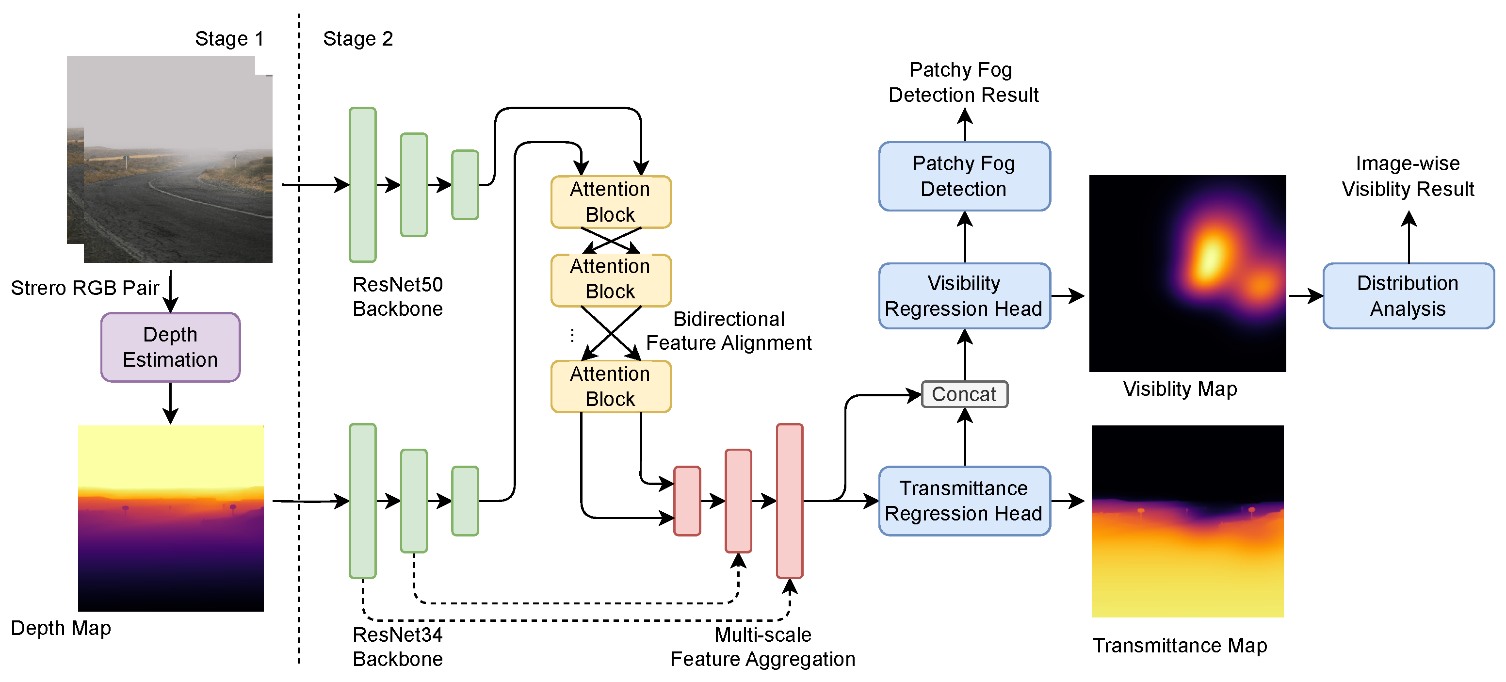
As shown in the Figure 4, the proposed network is divided into two stages. The first stage is the depth estimation module. To prevent the effects of fog on the depth estimation results, this module takes stereo images captured under clear-weather conditions as input and generates a disparity map. The corresponding depth map is calculated based on the intrinsic and extrinsic parameters of the camera. The second stage plays the role of the visibility estimation. It takes the depth map generated in the first stage and the foggy RGB image as inputs. These inputs are processed through feature extraction and feature fusion processes. Ultimately, this stage outputs a pixel-wise visibility map for the entire scene after multi-scale feature aggregation and regression.

Additionally, after the two-stage network, we add a patchy fog discriminator which analyzes the features from the previously generated pixel-wise visibility map to determine whether patchy fog is present in the scene.

5.2. Stage I: Scene Depth Perception

Inspired by the design of [43] and considering hardware efficiency, We adopt a hybrid design that combines a traditional stereo matching algorithm with a GRU-based cascaded recurrent stereo matching network for the depth estimation module. This advanced stereo matching architecture leverages rich semantic information while relying on geometric cues to ensure accurate scale, thereby addressing the challenge of accurately estimating disparity maps in diverse real-world scenarios.

We first employ traditional methods such as SGM [44] to perform cost construction and aggregation on features extracted by the CNN, obtaining a coarse initial disparity. Then, we employ a hierarchical network that progressively refines the disparity map in a coarse-to-fine manner. It utilizes a recurrent update module based on GRUs to iteratively refine the predictions across different scales. This design not only helps recover fine-grained depth details but also effectively handles high-resolution inputs. To mitigate the negative effects of imperfect rectification, we use an adaptive group correlation layer introduced by CREStereo [43], which performs feature matching within local windows and uses learned offsets to adaptively adjust the search region. It effectively handles real-world imperfections such as camera module misalignment and slight rotational deviations. This design enhances the network’s capability in handling small objects and complex scenes, significantly improving the quality of the final depth map.

During inference, to achieve a balance between speed and accuracy, initial depth estimation is performed at ${\displaystyle \frac{1}{16}}$ scale of the original resolution with a disparity range of 256, followed by iterative optimization conducted 4, 10, and 20 times at ${\displaystyle \frac{1}{4}}$, ${\displaystyle \frac{1}{8}}$, and ${\displaystyle \frac{1}{16}}$ scales of the original resolutions, respectively. Finally, based on the camera setup and intrinsic parameters, we convert the disparity map into a depth map.

5.3. Stage II: Pixel-Wise Visibility Measurement

In this section, we present the visibility estimation framework that effectively integrates RGB texture information and depth cues through a hybrid architecture combining convolution neural networks and transformer-based attention mechanisms [45]. As illustrated in Figure 4, our design consists of four key components: (1) a dual-branch feature extractor based on ResNet [46], (2) a bidirectional multi-modal feature alignment module, (3) a multi-scale feature aggregation module, and (4) a regression head for pixel-wise visibility map generation. This design enables comprehensive feature learning and precise visibility estimation by leveraging both local texture details and global contextual information.

5.3.1. Dual-Branch Feature Extraction

Our network utilizes two separate feature extractors to process RGB images and depth maps independently. The RGB branch is built upon a pre-trained ResNet50 architecture, while the depth branch adopts a pre-trained ResNet34 network modified to accept single-channel input, enabling it to effectively process depth maps. To ensure that the generated visibility maps are more consistent with the semantic and structural distributions, we utilize the feature outputs from the first to third layers of the depth branch to capture multi-scale spatial features.

5.3.2. Bidirectional Multi-Modal Feature Alignment

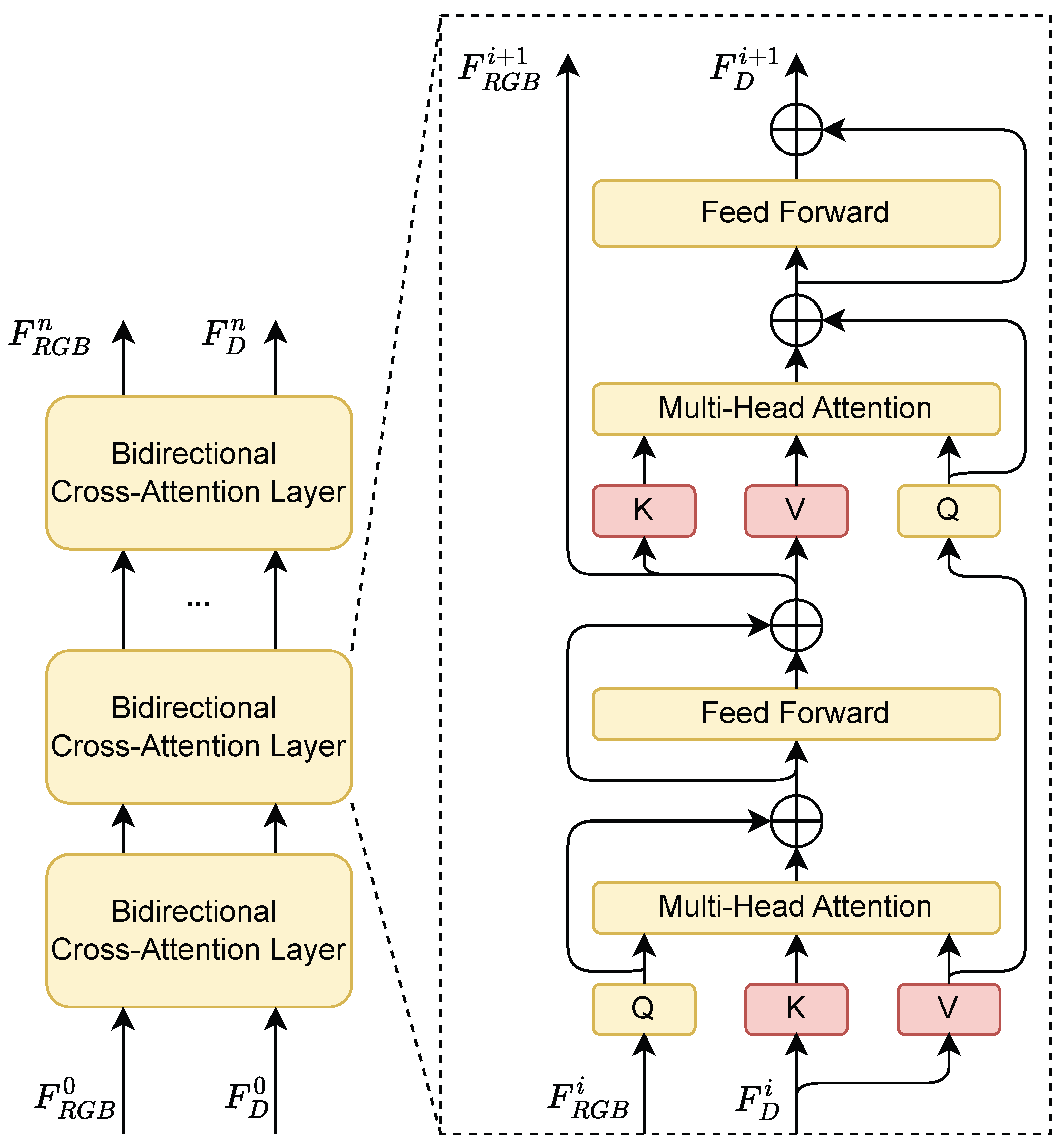
To integrate RGB and depth features, we introduce a feature alignment module involved cross-attention mechanism that fuses the structural and the semantic information from the scene, establishing a relationship between the transmittance and the depth. As illustrated in Figure 5, to achieve better aggregation of multi-modal features, we use a stacked BCB structure, allowing RGB semantic features and depth structural features to alternately query information from the other modality. The process of the stage i is described by Equation (7):

$$\begin{array}{cc}\hfill F_{RGB}^{i+1}& =Atten(Q_{RGB}^i,K_D^i,V_D^i)\hfill \\ \hfill F_D^{i+1}& =Atten(Q_D^i,K_{RGB}^{i+1},V_{RGB}^{i+1})\hfill \end{array}$$

(7)

Specifically, the fusion proceeds in two phases. In the first phase, the RGB feature $F_{RGB}^i$ is mapped as query $Q_{RGB}^i$, while the depth feature $F_D^i$ is mapped as the key $K_{RGB}^i$ and the value $V_{RGB}^i$. Multi-head attention computation followed by an MLP $Atten$ is applied after the feature mapping, which produces the RGB feature $F_{RGB}^{i+1}$ enriched with the depth information. In the second phase, on the other hand, the depth feature $F_D^i$ serves as the query $Q_D^i$, and the updated RGB features $F_{RGB}^{i+1}$ is used as the key and the value. Another round of attention computation is performed to generate the depth feature $F_D^{i+1}$ enhanced with RGB semantic information. This bidirectional interaction is repeated in a stacked manner, enabling progressive and mutual refinement of both modalities, thereby achieving more robust and context-aware feature representations.

5.3.3. Multi-Scale Feature Aggregation

Following the feature alignment module, we progressively merge the dual-branch features while gradually restoring the spatial resolution. Due to the strong correlation between visibility and metric depth, we further incorporate shallow-level features from the depth branch during the fusion process. To align the feature dimensions for feature aggregation, we apply $1\times 1$ convolution layers to project both RGB and depth features into a shared embedding space of dimension 512. This integration provides structural constraints on the visibility output, enhancing its geometric consistency. As illustrated in the Figure 6, the entire fusion process is accomplished through multiple fusion blocks. Each block consists of feature add, convolution with skip connections, and upsampling operations, enabling effective multi-scale feature refinement and facilitating the generation of accurate and spatially coherent visibility maps. Finally, we employ a ConvBlock consisting of multiple 2D convolution layers to further refine and aggregate the features.

5.3.4. Pixel-Wise Visibility Map Regression

At the final stage of the network, we design a regression head to estimate visibility. Due to its bounded range and invertible relationship with visibility, the extinction coefficient serves as a more suitable regression target than visibility itself. Therefore, we supervise the network using pixel-wise extinction coefficient predictions. The predicted visibility values is converted back during evaluation.

Furthermore, to impose stronger physical constraints on the network output, we introduce an auxiliary regression head that predicts a transmittance map. The transmittance map derived from the intermediate feature is jointly fed into the extinction coefficient regression head. During training, this transmittance prediction is supervised with ground truth transmittance, providing auxiliary supervision that regularizes the learning process and enhances the physical consistency of the estimated visibility. This multi-task design encourages the network to learn physically atmospheric models, thereby improving both accuracy and interpretability.

5.3.5. Visibility Map Distribution Analysis

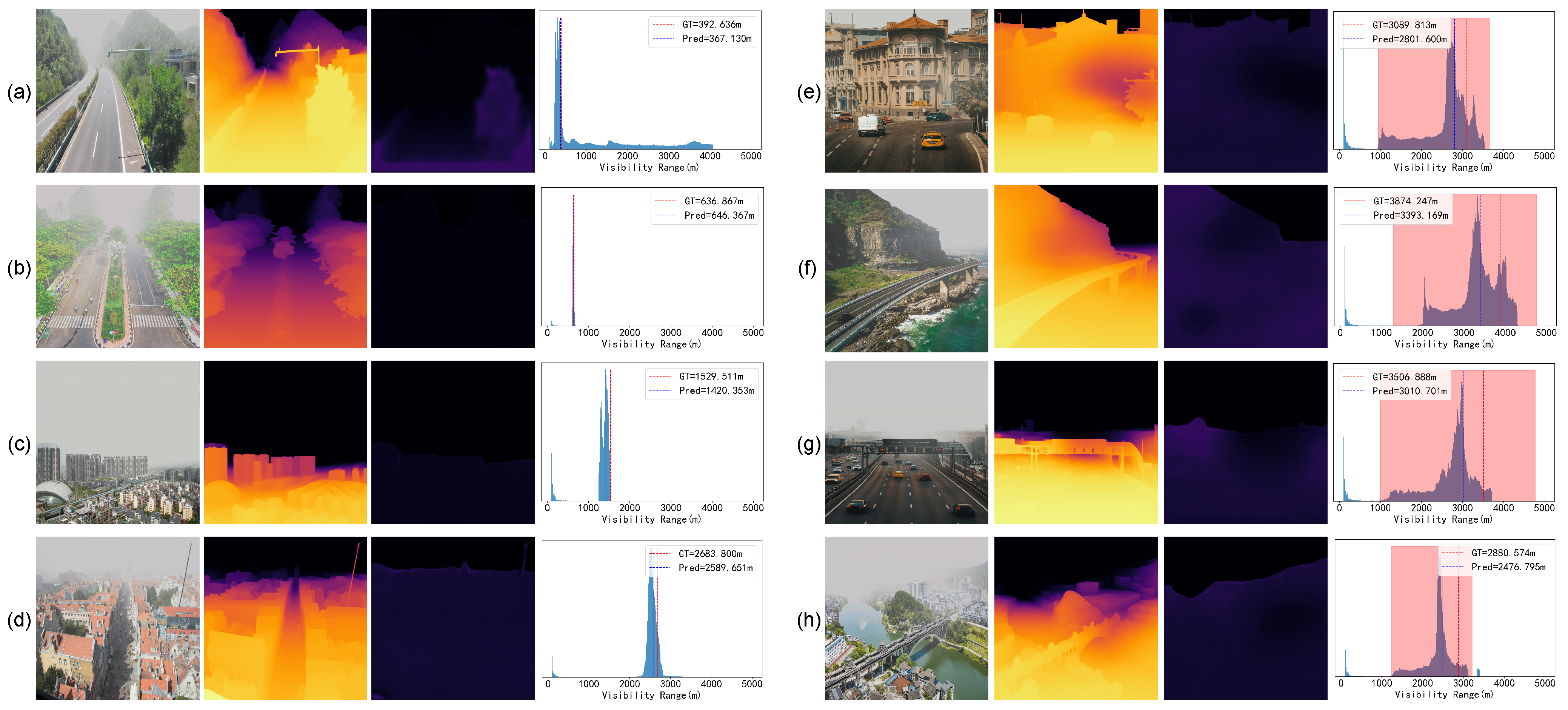
To evaluate the pixel-wise visibility results, we convert the extinction coefficient B predicted by the network into visibility V following the Equation (3). Additionally, to facilitate a more direct comparison with scalar visibility estimates from other methods and physical sensors, we convert our pixel-wise visibility results into image-wise visibility values. Unlike DMRVisNet [20], which directly uses a predefined data distribution to set thresholds, we analyze the distribution of the visibility results. Specifically, we compute the histogram of visibility map for 50 bins. Bins with counts less than 1% of the total are considered outliers and are filtered out. Further, we sort the histogram and select the farthest value among the top three bins as the final result. This method provides a more accurate representation of scene visibility by mitigating the impact of close objects, which lack rich transmittance information and could distort the visibility estimation. Finally, we clip the visibility values exceeding 5000 m to ensure the output remains within a physically meaningful and practically relevant range.

5.4. Patchy Fog Detection

In addition to generating a pixel-wise visibility map, we further propose a CNN-based patchy fog discriminator to determine whether patchy fog exists in the scene. Specifically, the discriminator takes the previously estimated visibility map combined with the transmittance map as input, which captures spatial variations in visibility across the scene. We design a lightweight CNN backbone to extract the representation indicative of fog distribution. To further enhance the model’s discriminative capability, we incorporate a global max pooling layer after each convolution block. Finally, we employ two fully connected layers to map the features to a binary classification indicating the presence or absence of patchy fog. This patchy fog detection module enables the system to not only estimate visibility quantitatively but also qualitatively perceive complex real-world fog distributions, improving situational awareness in practical transportation scenarios.

5.5. Loss Function

Considering that our network involves three distinct tasks—depth estimation, visibility estimation and patchy fog discrimination—we propose a multi-stage training manner correspondingly. In the first stage, we train the depth estimation module by feeding it RGB image pairs without fog augmentation and supervising it with depth ground truth. For the loss of the depth estimation, we refer to [43] and employ ground-truth depth to supervise the multi-scale depth outputs of the network following Equation (8). Specifically, for each scale $s\in \{{\displaystyle \frac{1}{4}},{\displaystyle \frac{1}{8}},{\displaystyle \frac{1}{16}}\}$, we resize the sequence of outputs from different iterations n, $\{f_1^s\dots f_n^s\}$ to the full prediction resolution. Subsequently, we compute the L1 loss of these multi-scale depth outputs with respect to the ground truth and obtain the final loss through a weighted summation.

$$L_{Depth}=\sum _s\sum _{i=1}^n{\left(0.9\right)}^{n-i}{L}_1(d_{gt}-Upsample\left(f_i^s\right))$$

(8)

In the second stage, we freeze the depth estimation component and proceed to train the network for visibility estimation. For images with stereo modalities, we use the depth inferred by the model from the first stage as the input for the depth branch. For the remaining images with monocular modalities, we utilize the depth ground truth provided by the dataset as input. Given that the proposed network produces multiple outputs, including a transmittance map, a pixel-wise visibility map, and a binary decision on the presence of patchy fog, we design a multi-task, weighted composite loss function that jointly optimizes all these objectives. Each component is normalized and scaled by a learnable or empirically tuned weight to balance the contribution of each task during training.

Specifically, the overall loss function is formulated as a weighted sum of these individual loss terms, as shown in Equation (9):

$$L_{all}={\lambda }_1{L}_{vis}+{\lambda }_2{L}_{det}$$

(9)

where $L_{vis},L_{det}$ denote the visibility regression loss and the patchy fog classification loss, respectively. ${\lambda }_1,{\lambda }_2$ are empirically tuned weights to balance the contribution of each task during training.

For visibility estimation, we observe a significant correlation among extinction coefficient map B, depth map D, and transmittance map T. Moreover, the transmittance map plays a crucial role in dehazing foggy images. To leverage these physical relationships, we introduce a semi-supervised loss function with strong physical constraints. The overall objective is formulated as a weighted sum of the extinction coefficient regression loss $L_B$, the transmittance regression loss $L_T$, the transmittance reconstruction loss $L_{reT}$, and the dehazed image reconstruction loss $L_{reI}$. The L1 loss is employed to uniformly measure the loss between the estimated results and the corresponding ground truths for each term. The loss function is defined as Equation (10):

$$\begin{array}{cc}\hfill L_B& =L_1(-{\displaystyle \frac{ln\left(T\right)}{D}},\widehat{B})\hfill \\ \hfill L_T& =L_1(T,\widehat{T})\hfill \\ \hfill L_{reT}& =L_1(e^{-\widehat{B}D},\widehat{T})\hfill \\ \hfill L_{reI}& =L_1({\displaystyle \frac{I-I_{\infty }(1-\widehat{T})}{\widehat{T}}},I_0)\hfill \\ \hfill L_{Vis}& ={\delta }_1{L}_B+{\delta }_2{L}_T+{\delta }_3{L}_{reT}+{\delta }_4{L}_{reB}\hfill \end{array}$$

(10)

where ${\delta }_{1\dots 4}$ are hyperparameters that balance the transmittance loss and the visibility loss, and it varies dynamically during training. To align with the distribution used during dataset generation and enhance model generalization, we randomly sample the value of $I_{\infty }$ from the same interval as used in data generation step to introduce small perturbations during training.

For $L_{det}$, we employ the binary cross-entropy loss, where $y_i$ denotes the ground-truth label of sample, and $\widehat{y_i}$ represents the model’s prediction result for the presence of patchy fog in per sample.

$$L_{det}=-{\displaystyle \frac{1}{N}}\sum _{i=1}^n[y_{i}log\left(\widehat{y_i}\right)+(1-y_i)log(1-\widehat{y_i})]$$

(11)

6. Experiment

In this section, we first present the implementation details of the training and evaluation setups. We then conduct both quantitative and qualitative evaluations of the model’s visibility estimation capability on the synthetic datasets. Specifically, we demonstrate the accuracy of the model for detecting patchy fog patches. We also present ablation studies on the network modules and loss function components to analyze their contributions to overall performance. In addition, we further validate the effectiveness of our approach by deploying the algorithm on an embedded device and comparing its estimates with real-world measurements from an FSVM, as well as further analysis in places with different fog scenarios.

6.1. Implementation Details

6.1.1. Data Augmentation

To validate the performance of the proposed network, we randomly split the dataset into a training set, a validation set, and a test set at a ratio of 7:2:1, respectively. During the training phase, we apply a series of data augmentation to the input data. To ensure that the images do not predominantly consist of foggy, texture-less sky regions or overly close ground regions, we perform random cropping on both the input images and corresponding ground truth, selecting 75% of their original size. These cropped patches are then uniformly resized to a resolution of 640 × 640. To adapt to varying camera exposure and color conditions, we randomly adjust the brightness, contrast, saturation, and hue of the RGB images by ±10%, ±15%, ±15%, ±5%, respectively.

6.1.2. Hyperparameter Setting

During the training phase, we use the AdamW [47] optimizer with an initial learning rate of 5 × ${10}^{-4}$ and a weight decay of 1 × ${10}^{-2}$. The batch size was set to 16. The learning rate was decayed in a step-wise manner, reduced to half of its current value every 10 epochs. The model was trained for a total of 80 epochs on four NVIDIA GeForce GTX 2080 Ti GPUs (Nvidia Corporation, Santa Clara, CA, USA). For stage 1, the depth estimation module is trained for 16 epochs. For stage 2, we freeze the weights of the depth estimation branch and jointly train the visibility estimation module and the patchy fog detection module for 80 epochs. We set ${\lambda }_1=1.0$ and ${\lambda }_2=0.4$ to balance the contributions of visibility estimation and patchy fog detection in the overall loss function, ensuring effective joint training of both tasks. In addition, we adopt a progressive training strategy for visibility estimation. Specifically, we keep the ${\delta }_1=0.4$ and ${\delta }_2=1.0$ fixed throughout the entire training process. During the first 20 epochs, we supervise only the transmittance map loss by setting ${\delta }_3$ and ${\delta }_4$ in the $L_{vis}$ to 0, allowing the network to fully learn the semantics and structure of the visibility measurement. In the remaining training, we set ${\delta }_3$ to 0.2 and ${\delta }_4$ to 0.1, guiding the visibility predictions to adhere to the physical relationship.

6.2. Results Comparison on the Synthetic Datasets

6.2.1. Quantitative Results

As shown in the Figure 7, we split the test set into uniform fog scenes and patchy fog scenes, and evaluate at both pixel-level and image-level to comprehensively assess the performance of our method under different visibility conditions. The red dashed lines in the figures indicate the correspondence between predictions and ground truths. It can be observed that within the test range, our results are distributed close to the ground-truth values, except for a few instances with very close or outlier inputs leading to prediction failures. These failures in prediction arise primarily from unreasonable camera placements in the collected data, resulting in images dominated by either excessively close buildings or sky, thereby causing a loss of depth information. Direct estimating on such semantically ambiguous regions, which lack reliable depth context, can lead to erroneous results, as highlighted by the red boxes in Figure 7. We manually identified and excluded these outliers, which constituted approximately 1.3% of the test dataset. Furthermore, to evaluate the robustness and stability of our model under realistic inference conditions, we perform stochastic inference during testing by applying lightweight input perturbations, including specifically small Gaussian noise and color jitter. For each sample, we conduct five repeated forward passes and compute the standard deviation of the resulting metrics across these runs as an indicator of prediction stability. Following the removal of these outlier inputs and the perturbation-based evaluation, on the patchy fog dataset, we obtain an AbsRel of $0.086\pm 0.006$, SqRel of $0.012\pm 0.006$, RMSE of $236.273\pm 9.911$, with a maximum distance error of 1166.941 m ± 153.595 m. While on the uniform fog dataset, the results are an AbsRel of $0.056\pm 0.004$, SqRel of $0.005\pm 0.002$, RMSE of $148.126\pm 8.935$, and a maximum distance error of 1002.103 m ± 59.072 m. With an increase in the ground-truth distance, the error margin also increases accordingly, which amplifies the RMSE value. The results obtained under patchy fog conditions exhibit greater dispersion compared to those from uniform fog, highlighting the limitation of using a single scalar value to represent visibility in such complex environments. This further underscores the advance of our pixel-wise visibility estimation approach, which captures the spatial variability of visibility and provides a more reliable assessment of visibility under non-uniform fog conditions.

Furthermore, we compare our method with other visibility estimation approaches to demonstrate its effectiveness. We select FACI [20] as the benchmark dataset to evaluate the second stage of our model against regression-based visibility estimation methods. Our method was retrained on this dataset using the aforementioned training protocol for 60 epochs, and then evaluated for performance comparison. As shown in

Table 2. Quantitative results on FACI Dataset [20] with different visibility ranges. The best results are marked bold.

Method	AbsRel	SqRel	RMSE
DMRVisNet [20]	0.170	0.051	93.113
GRNN [12]	0.279	0.134	156.591
Ours	0.098	0.021	43.984

, our method achieves the best performance. This result highlights the effectiveness of leveraging metric-scale depth and the robustness of our fusion network design. Moreover, it indicates that our physically constrained, progressive supervision strategy contributes to more reliable visibility predictions, especially under challenging and non-uniform fog conditions.

For other mainstream visibility estimation methods [12,48,49] whose datasets or code are not fully publicly available, we ensure a fair comparison by evaluating our method on subsets of our dataset that match the visibility ranges covered by those methods. Specifically, we analyze the reported operational visibility intervals in each respective study and extract corresponding segments from our high-quality, real-world captured data to form evaluation splits with similar statistical distributions. This allows us to simulate the testing conditions of prior works as closely as possible. Furthermore, to facilitate direct comparison with classification-based methods, we map the continuous visibility predictions from our model to discrete visibility level labels. Specifically, we define five visibility classes corresponding to the following ranges: (0, 200 m], (200 m, 500 m], (500 m, 1000 m], (1000 m, 2000 m], and (2000 m, 5000 m]. The predicted visibility values are assigned to these categories, and we compute the classification accuracy as the evaluation metric. As shown in the

Table 3. Quantitative results of the visibility estimation across different datasets with similar visibility ranges.

Method	Dataset	Range (m)	Accuracy (%)
Zou et al. [50]	Private	0–1000	92.0
Visor-net [49]	FHVI	0–1000	87.8
Ours	Ours	0–1000	87.3
Liu et al. [48]	Private	0–3000	87.6
Ours	Ours	0–3000	90.8
Ours	Ours	0–5000	93.1

, our method achieves competitive performance compared to existing approaches, demonstrating the effectiveness of our framework in categorical visibility assessment. This evaluation further validates the robustness and generalization capability of our approach across different visibility ranges.

Furthermore, to thoroughly evaluate the accuracy and error characteristics of visibility categorization, we analyze the rates of missed detections and false alarms for each visibility class. For a given visibility class $V{C}_i$, a sample belonging to $V{C}_i$ is considered a false negative if the predicted result falls outside its interval. Conversely, a sample is counted as a false positive for $V{C}_i$ if the ground truth belongs to a different class but the estimated visibility is assigned to $V{C}_i$. Based on this statistical method, we calculated the classification performance of different visibility ranges. As shown in the

Table 4. Classification performance of the visibility estimation across different visibility ranges.

Visibility Class	Visibility Range (m)	Accuracy (%)	Precision (%)	Recall (%)
1	(0, 200 m]	99.9	100.0	92.9
2	(200 m, 500 m]	90.5	87.3	91.7
3	(500 m, 1000 m]	94.9	92.0	86.2
4	(1000 m, 2000 m]	92.0	93.8	89.9
5	(2000 m, 5000 m]	93.2	91.7	95.4

, our method achieves high accuracy, precision, and recall across all classes, demonstrating its effectiveness in accurately categorizing visibility levels. This analysis provides deeper insights into the model’s performance, highlighting its reliability in both detecting true visibility conditions and minimizing erroneous classifications. Notably, our method outputs continuous, absolute-scale visibility estimates. In practical deployment, the categorization thresholds can be flexibly adjusted according to domain-specific requirements, enabling adaptation to different operational standards without retraining the model.

We evaluate the effectiveness of the patchy fog discriminator. As shown in the PR curve in Figure 8, our method achieves an AUC of 0.959, demonstrating strong classification performance. We further determine the optimal threshold based on the F1 score, obtaining a maximum F1 value at a threshold of 0.928. At this optimal threshold, the classifier achieves a recall of 1.0 and a precision of 0.865, indicating high sensitivity in detecting patchy fog instances while maintaining prediction reliability. These results validate the robustness and accuracy of our patchy fog detection mechanism.

6.2.2. Qualitative Results

Figure 9 provides an intuitive presentation of the visibility estimation results. For qualitative evaluation, we select representative cases with diverse scenes covering a wide range of visibility values, including both uniform and patchy fog conditions. Since the original visibility maps do not relate to the texture and are challenging to illustrate clearly due to the scale of the value, we offer a more straightforward view of the visibility estimation through histogram statistics of pixel-wise visibility maps. In these histograms, image-wise values of the ground truth and the predicted results are indicated with red and blue dashed lines, respectively. Furthermore, pixel-level transmittance results are provided to further substantiate the analysis.

It can be observed that with the help of the absolute metric depth input, the predicted transmittance map is fairly accurate, with object edges being clear as well. This highlights the accuracy of the visibility estimations, especially underlining the clarity of object edges in the predicted transmittance maps, which is crucial for reliable visibility estimation. Regarding the distribution of visibility, in scenarios with uniform fog, the visibility distribution is compact and centers around the ground truth. For patchy fog cases, visibility distribution mainly clusters between the maximum and minimum ground-truth visibility. Notably, surfaces such as the ground and closer objects within the scene often result in low peaks in the histogram statistics of visibility estimation due to a lack of transmittance information, which could potentially impact the network performance. This phenomenon indicates the challenge in accurately estimating visibility for elements at closer distances. Meanwhile, it further demonstrates that our selected image-wise visibility is representative, as indicated by the blue dashed line in the figure. Compared to using simple average, it is closer to the ground truth represented by the red dashed line, thereby providing a more accurate representation of the image-wise visibility.

6.2.3. Ablation Studies

We conduct ablation studies on the impact of different numbers of BCBs on visibility estimation performance.

Table 5. Impact of the number of BCBs on visibility estimation performance. The best results are marked bold.

Num of BCB	AbsRel	SqRel	RMSE	Params (MB)
0	0.140	0.050	335.163	22.957
1	0.142	0.027	364.078	23.484
2	0.104	0.019	252.011	24.011
3	0.069	0.008	187.246	24.538
4	0.087	0.014	210.170	25.066

presents the regression results for configurations ranging from zero to four stacked BCB blocks, along with their respective model params. As shown, under the same training settings and hyperparameters, using three stacked BCB blocks achieves the best performance, offering a favorable trade-off between accuracy and model complexity. Employing more blocks leads to a slight performance degradation, which indicates difficulty in optimization due to increased training difficulty. Surprisingly, the model without any BCB block performs slightly better than the one with a single BCB, which may suggest that a single block is insufficient to capture meaningful cross-view dependencies and introduces additional noise.

In addition, we further investigate the contribution of different components in the loss function to network training. We conduct ablation studies to evaluate the impact of including or removing each individual term on the performance of visibility estimation.

Table 6. Impact of the design of the loss function on visibility estimation performance. The best results are marked bold.

${\mathit{L}}_{\mathit{B}}$	${\mathit{L}}_{\mathit{T}}$	${\mathit{L}}_{\mathit{reT}}$	${\mathit{L}}_{\mathit{reI}}$	AbsRel	SqRel	RMSE
✓				0.115	0.026	318.774
✓	✓			0.095	0.015	252.211
✓	✓	✓		0.080	0.012	213.283
✓	✓	✓	✓	0.069	0.008	187.246

demonstrate that the network’s estimation error decreases progressively with the inclusion of the regularization terms. In contrast, directly supervising the extinction coefficient leads to a significant increase in error, which suggests that the extinction coefficient is sensitive to noise and difficult to learn in a fully supervised manner. This observation further validates the effectiveness of our designed transmittance-assisted training and multi-component loss function, which incorporates semantic, structural, and physical constraints to guide the visibility estimation task from complementary perspectives. By balancing these supervisory signals, our approach achieves more robust and accurate predictions without overfitting to potentially noisy or ill-posed targets.

6.3. Results Analysis in the Real-World Environment

6.3.1. System Implementation

To further validate our work and demonstrate the effectiveness of the proposed algorithm, we deploy the network on an RK3588 (Rockchip Electronics Co., Ltd., Fuzhou, China) embedded device. This device features an RK NPU (Rockchip Electronics Co., Ltd., Fuzhou, China) and a Mali-G610 mobile GPU (Arm Limited, Cambridge, United Kingdom) as co-processors, providing strong capabilities for parallel computing and deep learning acceleration. We implement the initial depth estimation in Stage 1 using OpenCL for efficient execution on the GPU. For the iterative refinement of depth estimation, we leverage both OpenCL and TVM [51] to optimize performance and flexibility. The visibility estimation network and patchy fog detection network are compiled and deployed using RKNN, ensuring high efficiency and low latency. After completing the above edge-device optimizations, a single forward pass during inference takes approximately 200 ms. This rate is significantly faster than the typical temporal dynamics of weather changes, which enables real-time visibility measurement.

Furthermore, as illustrated in Figure 10a, we integrate the embedded device with a stereo camera and a pan-tilt platform to construct a complete visibility estimation system, which provides the capability of absolute metric depth estimation and 360° rotational observation. We measured the power consumption of the entire device under both idle and active states. In the idle state, the power consumption is approximately 0.3~0.7 W, while in the active state, it ranges from 5.7~6.5 W. This low power profile demonstrates excellent energy efficiency and makes the system well-suited for long-term outdoor deployment in remote or infrastructure-limited environments. As illustrated in Figure 10b, the system is mounted at a fixed position alongside an FSVM, depicted in Figure 10c. The two devices are placed approximately 3 m apart horizontally and about 1 m apart vertically, which avoids mutual interference between sensors while ensuring both operate under similar atmospheric conditions. As shown in Figure 10d, we oriented the camera toward a direction with an open field of view and rich scene texture, ensuring reliable semantic and depth information for visibility estimation.

We record the outputs from our device and the FSVM every minute for analysis. Notably, the FSVM is a commonly used instrument in atmospheric and transportation applications for visibility estimation, which serves as a valuable reference for evaluating the real-world performance of our method. However, as illustrated in Figure 10d, the FSVM primarily measures visibility in the immediate vicinity of the sensor, resulting in a point-based perception with very limited spatial coverage. In contrast, our method estimates visibility across the entire camera field of view. Despite differences in sensing field of view and range, both sensors measure the same physical quantity. Therefore, we analyze the trend and temporal consistency between the two sets of estimates rather than their absolute accuracy, focusing on whether both systems capture visibility changes, such as fog onset, dissipation, or sudden fluctuations, in a synchronized and qualitatively aligned manner.

6.3.2. Result Comparison with FSVM

Figure 11 presents a comparison between our method and the FSVM under different illumination conditions and visibility scenarios. Specifically, in scenario (a), our estimates closely align with the measurements from the FSVM for the majority of the time, demonstrating the effectiveness of our method in accurately estimating visibility under real-world conditions. In scenario (b), our vision-based approach directly perceives the reduction in visibility from the scene, while the FSVM only reflects changes after the atmospheric conditions at its physical location have changed, resulting in a measurement lag. This highlights the superior responsiveness of our method. Scenario (c) corresponds to a rainy period, during which water droplets on the camera lens degrade image quality and adversely affect our visibility estimation. In scenario (d), the scene remains visually stable, and our method produces consistent and smooth visibility estimates accordingly. In contrast, the FSVM exhibits fluctuations due to localized atmospheric disturbances near the sensor. Overall, our method delivers accurate visibility estimates, promptly captures environmental changes, and benefits from a large field of view that enhances result stability. However, it is susceptible to performance degradation caused by lens contamination or adverse weather affecting image quality. This analysis underscores both the advantages and current limitations of our vision-based approach in real-world deployment.

6.3.3. Result Analysis in Diverse Fog Conditions

As shown in Figure 12a, we further deployed a test site on a highway in a high-altitude region of Guizhou Province, China to evaluate our system under real-world conditions with diverse visibility levels and fog distributions. In Figure 12b–e, we present typical scenarios including uniform fog or patchy fog under high visibility or low visibility, respectively. For each scenario, we provide the corresponding transmittance map, visibility distribution histogram, estimated visibility value, and confidence in the presence of patchy fog. As can be seen, our method consistently captures the spatial structure and intensity of visibility variations across different conditions, demonstrating robustness in complex real-world environments. The patchy fog discriminator accurately identifies the presence of patchy fog, even in challenging low-visibility scenarios. These results validate the practical applicability of our approach for real-time visibility monitoring and patchy fog detection in transportation settings.

7. Conclusions

In this work, we propose a two-stage network for accurate visibility estimation using stereo images. Our method generates pixel-wise visibility maps and introduces a novel mechanism for detecting patchy fog, significantly improving traffic safety under low-visibility conditions. We also develop an automatic pipeline for creating synthetic foggy images, enhancing model training and evaluation. Experimental results on both synthetic and real-world datasets demonstrate advanced performance in visibility estimation and patchy fog detection. Furthermore, we deploy our method on an embedded device to construct a visibility monitoring system. We further analyze the performance of our device in comparison with the FSVM under various weather conditions, validating its effectiveness for practical deployment in intelligent transportation scenarios.

In our future work, we will optimize the network architecture to achieve more accurate visibility estimates over longer distances. Additionally, we aim to refine the stitching of visibility estimates from multiple viewing angles, enabling the reconstruction of detailed panoramic visibility maps and more comprehensive patchy fog distribution. Furthermore, we plan to integrate data from multiple spatially distributed sensors to collaboratively estimate large-scale fog fields, with the goal of monitoring complex environments such as airports and other critical infrastructure.