Abstract
Fluctuations in precipitation usually affect the ecological environment and human socioeconomics through events such as floods and droughts, resulting in substantial economic losses. The high-resolution models in the Coupled Model Intercomparison Project Phase 6 (CMIP6) are vital for simulating precipitation patterns in China; however, significant uncertainties still exist. This study utilized the quantile mapping (QM) method to correct biases in nine high-resolution Earth System Models (ESMs) and then comprehensively evaluated their precipitation simulation capabilities over the Chinese mainland from 1985 to 2014. Based on the selected models, the Bayesian Model Averaging (BMA) method was used to integrate them to obtain the spatial–temporal variation in precipitation over the Chinese mainland. The results showed that the simulation performance of nine models for precipitation from 1985 to 2014 was significantly improved after the bias correction. Six out of the nine high-resolution ESMs were selected to generate the BMA ensemble model. For the BMA model, the precipitation trend and the locations of significant points were more closely aligned with the observational data in the summer than in other seasons. It overestimated precipitation in the spring and winter, while it underestimated it in the summer and autumn. Additionally, both the BMA model and the worst multi-model ensemble (WMME) model exhibited a negative mean bias in the summer, while they displayed a positive mean bias in the winter. And the BMA model outperformed the WMME model in terms of mean bias and bias range in both the summer and winter. Moreover, high-resolution models delivered precipitation simulations that more closely aligned with observational data compared to low-resolution models.
1. Introduction
Precipitation is a crucial element of the climate system and acts as a key connection among the atmosphere, hydrosphere, and biosphere. Changes in precipitation and climate have significant impacts on human society, ecosystems, and local environments [1]. These impacts are primarily manifested through the appearance of extreme precipitation events like floods and droughts, which cause extensive economic losses [2]. China boasts a vast territory and complex topography, which makes the variability of its water resources, climate, and precipitation particularly significant. Consequently, accurate prediction of precipitation changes is crucial for agricultural production, economic development, and environmental preservation within the country.
Current methods for estimating precipitation primarily rely on satellite data, ground station measurements, and climate model outputs [3]. Satellite data, collected through remote sensing technology, offers global-scale observations of precipitation. It offers several advantages, including extensive coverage, high spatiotemporal resolution, and real-time availability, which facilitate global-scale precipitation monitoring and short-term forecasting [4]. Ground station data consists of precipitation observations gathered from meteorological stations located on the ground. While it is renowned for its high precision, the uneven distribution and limitations of station locations result in constrained spatial coverage, particularly in remote areas and over oceans [5,6]. Model data refer to precipitation predictions generated by various weather and climate models [7]. These models are built upon physical equations of the atmosphere and are informed by meteorological observations. By simulating atmospheric processes, they provide forecasts of precipitation for future periods [8]. Among the three methods, model data offer distinct advantages due to their capacity to produce future forecasts. This capability is critically important for predicting precipitation trends and enhancing regional disaster prevention and mitigation strategies. Specifically, model data support early warning systems, facilitate long-term planning, and improve operational responses to extreme weather events. Furthermore, they integrate multidisciplinary knowledge from atmospheric science, fluid dynamics, and numerical computation, enabling continuous improvement in forecast accuracy and spatiotemporal resolution through data assimilation and machine learning techniques [9,10].
The Coupled Model Intercomparison Project (CMIP) was initiated by the World Climate Research Programme (WCRP) to address emerging scientific questions in the field of climate change while also providing critical data support for achieving the research objectives outlined in WCRP’s Grand Science Challenges. The Earth System Model (ESM) is a key component of the CMIP and offers a thorough simulation of the interactions among different elements of the earth system [11]. Consequently, ESMs are frequently utilized for climate simulation and prediction [12,13]. However, since its inception, the ESM has been affected by uncertainties and errors [14]. For instance, some studies in CMIP3 ESMs have indicated that the simulated precipitation tends to be underestimated in Eastern China and overestimated in the Yangtze River Basin [15,16]. In Miao et al.’s study, they used CMIP3 data to simulate rainfall and temperature in China and recommended using it with caution due to its poor simulation performance [17]. In comparison, CMIP5 models present certain improvements over CMIP3 models [18]. Within CMIP5, the simulation of convective rainfall has been enhanced through the optimization of convective parameterization [19,20]. However, these models still suffer from significant uncertainties and errors [21,22]. Currently, the CMIP initiative has entered its sixth phase (CMIP6), aiming to further reduce uncertainties in ESMs and enhance the accuracy of climate projections [23]. Compared to CMIP5, CMIP6 ESMs provide more advanced climate prediction data by involving a broader range of model types developed by a greater number of research institutions, incorporating complex physical processes, reducing long-term model biases through improved parameterization schemes and observational constraints, and increasing spatial resolution [14,24,25,26].
Over the past two decades, the resolution of ESMs has gradually improved alongside the advancement of the CMIP. The horizontal resolution of CMIP3 models’ data for the atmosphere was primarily 250 km and 1.5° for the ocean [15]. The atmospheric horizontal resolution of CMIP5 models had increased to 150 km, and the oceanic resolution had improved to 1° [27]. The HighResMIP project was incorporated into CMIP6, featuring a horizontal resolution of about 0.25°, which was rarely seen in CMIP3 and CMIP5 [28]. This project seeks to evaluate the advantages of higher resolution in improving climate model performance. The simulation capacities of CMIP models for the East Asian summer monsoon have progressively improved from CMIP3 to CMIP5 to CMIP6, corresponding with an increase in spatial resolution [29,30].
Moreover, individual global climate models (GCMs) often exhibit significant biases and uncertainties in simulating precipitation patterns and extremes. These uncertainties stem primarily from differences in model structures and the internal variability of the climate system [31]. To address this, ensemble methods, like multi-model ensemble averaging (MME), are employed to reduce uncertainties across different models. The MME approach is a common strategy to mitigate these uncertainties by averaging across models [32]. For instance, the model is capable of simulating winter temperature and precipitation in complex terrain using MME [33]. However, a critical limitation of the simple MME is that it assigns equal weight to all models, regardless of their individual performance in simulating the regional climate of interest [34]. To overcome this limitation, more advanced methods, such as Bayesian Model Averaging (BMA), have also been utilized in climate change and hydrological predictions [35]. The BMA method employs the Expectation–Maximization (EM) algorithm to calculate the weights among different models, assigns unequal weights to these models, and uses them to generate more reasonable estimations by weighting simulation results from multiple models [36]. BMA not only offers predictions that are more accurate than an individual model in the ensemble but also infers reasonable model probabilities [37]. Miao et al. compared the MME and BMA using eight models from CMIP5 and found that the simulation performance of BMA outperformed that of both MME and individual models [17]. However, there is limited research on using the BMA approach to simulate precipitation in China based on CMIP6 ESMs, particularly with high-resolution models. In addition, correcting bias is necessary before the BMA.
This study quantifies the best simulations of Chinese precipitation from nine CMIP6 high-resolution models and analyzes their spatiotemporal characteristics. The specific contents are as follows: (1) The Quantile Mapping (QM) method was utilized to correct bias on the nine models. (2) The best-performing models were chosen based on the correlation coefficient (CC), root mean square error (RMSE), and Taylor skill score (S), and then the simulation output was generated using the BMA method. (3) The spatiotemporal features and attribution of Chinese precipitation were analyzed in conjunction with changes in related climatic variables. In accordance with these goals, the structure of this study is outlined below: In Part 2, there is a detailed overview of the datasets and methods used in the research. The methods employed include the QM method, evaluation metrics, Mann–Kendall trend test (M-K), and BMA approach. Part 3 outlines the results of the study, and Parts 4 and 5 denote the discussion and conclusions, respectively.
2. Materials and Methods
2.1. Study Area
In this study, we concentrated on the Chinese mainland to examine variations in precipitation across different regions. The Chinese mainland is divided into eight sub-areas primarily based on administrative divisions and the characters of the monsoon climate of China. The division of the four sub-areas in Eastern China roughly considers the north-ward advances in the East Asian summer monsoon as well as administrative divisions. The south of Western China is divided mainly based on administrative divisions, attempting to make Southwest China cover as many regions of Yunnan, Guizhou, Sichuan, and Chongqing as possible. According to the fact that there are precipitation increasing and decreasing regions, Northwest China is divided into east and west sub-areas [36,37]. These regions are as follows: (1) Northeast China (NEC) (north of 42.5° N, east of 110° E), (2) North China (NC) (35° N–42.5° N, east of 110° E), (3) the middle and lower reaches of the Yangtze River and the Huaihe River Valley, briefly Jianghuai (JH) (27.5° N–35° N, east of 107.5° E), (4) South China (SC) (south of 27.5° N, east of 107.5° E), (5) Southwest China (SWC) (south of 35° N, 97.5° E–107.5° E), (6) the east of the Tibetan Plateau (TP) (south of 35° N, west of 97.5° E; because of the lack of stations in the west of the plateau, the analysis results of this area only represent the situations in the east of the plateau), (7) the west of Northwest China (WNW) (north of 35° N, west of 97.5° E), and (8) the east of Northwest China (ENW) (north of 35° N, 97.5° E–110° E). The specific study area and its subdivisions are depicted in Figure 1.
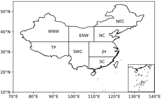
Figure 1.
Partitioning of the study area and its eight subregions.
The eight subregions of China exhibit not only distinct spatial patterns in geography but also complex and diverse topographic and climatic characteristics.
NEC: This region is characterized by plains and mountains. It experiences a temperate monsoon climate, with cold, dry winters and warm, rainy summers. Annual precipitation decreases from southeast to northwest.
NC: Dominated by the North China Plain, it also includes the eastern part of the Loess Plateau and the Taihang Mountains. The climate is temperate monsoon with concentrated summer rainfall. Frequent spring droughts and water resource shortages are prominent issues.
JH: Located in the lower reaches of the Yangtze and Huai rivers, this area consists of alluvial plains and surrounding hills, with extensive river networks and numerous lakes. It has a subtropical monsoon climate, featuring pronounced Meiy events. Abundant summer rainfall often leads to flooding.
SC: This region is composed of hills, low mountains, and coastal plains, with karst landscapes being common. The climate is tropical to subtropical monsoon, with high temperatures, abundant rainfall, a long rainy season, and frequent typhoon activity.
SWC: This area includes the Sichuan Basin, the Yunnan–Guizhou Plateau, and the southern section of the Hengduan Mountains, with highly varied terrain. The climate is influenced by the Indian monsoon and topographic uplift, resulting in significant regional differences: the basin is hot and humid, while the plateau exhibits distinct vertical climatic zones.
TP: This transition zone between the Tibetan Plateau and the Sichuan Basin/Yunnan–Guizhou Plateau features alternating high mountains and deep valleys with dramatic elevation changes. The climate is high-altitude and cold, with precipitation influenced by monsoons and topography. The winters and springs are dry and cold, while the summers are cool and humid.
WNW: This subregion comprises the Tarim Basin, Junggar Basin, and the Tianshan and Altai Mountains. It has a typical temperate continental arid climate, with scarce precipitation, high evaporation, large diurnal temperature variations, and a landscape of deserts and oases.
ENW: Covering most of the Loess Plateau, western Inner Mongolia Plateau, and the Hexi Corridor, this area has an arid to semi-arid climate. Precipitation decreases from east to west, and wind–sand activities are frequent, making the ecosystem highly vulnerable.
2.2. Data
In this study, a daily precipitation dataset spanning from 1985 to 2014 was utilized. This dataset encompasses 2839 grid points within and surrounding China (https://doi.org/10.11888/Atmos.tpdc.300523) [38]. The dataset was developed by employing an improved inverse distance weighting method combined with the machine learning-based light gradient boosting machine (LGBM) algorithm. The dataset features a spatial resolution of 0.25° by 0.25° and a daily temporal resolution. In this study, it is abbreviated as CHM.
For the multi-model precipitation data, we selected nine models of HighResMIP (https://data.ceda.ac.uk/badc/cmip6/data/CMIP6/HighResMIP) (accessed on 9 July 2024) and nine low-resolution models (https://aims2.llnl.gov/search/) (accessed on 18 July 2024). These high-resolution models possess a spatial resolution of 25 km and a monthly temporal resolution. Table 1 lists the names and sources of the eighteen datasets.

Table 1.
Details of nine CMIP6 high-resolution and low-resolution ESMs used in this research.
2.3. Method
In order to make comparison easier, this study applied masking and bilinear spatial interpolation methods to standardize all model data onto a 0.25° by 0.25° grid. To address the discrepancies between the model outputs and observed data, we utilized the QM method to perform bias correction at each grid point for different months, aiming to reduce this bias. After bias correction, statistical indicators are calculated to compare each model with the observed data. The best-performing models are selected based on these statistical indicators to generate the BMA. Subsequently, the M-K test is employed to assess the BMA precipitation trend in the analysis. The procedural flowchart of the research method is illustrated in Figure 2.
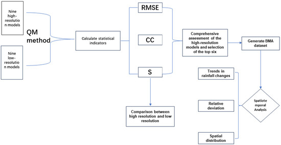
Figure 2.
Flowchart of this study.
2.3.1. QM Method
The QM method is commonly employed to correct biases when contrasted with observational data [46]. The QM method is a frequency distribution-based correction technique that assumes that the observed and simulated precipitation follow similar frequency distributions [47].
The core of the QM method lies in establishing a functional relationship between observational and simulated data from the historical period, which is then used to correct simulated values. Therefore, it can be applied not only to correct historical data but also to correct precipitation in future simulations by leveraging the distribution function relationship derived from the historical data. The principle for correcting historical data is as follows:
where is the historical simulated precipitation, is the cumulative function (CDF) of the historical model simulations, is the inverse CDF (quantile function) of the historical observations, is the bias-corrected precipitation value, m represents the model, o represents the observe data, and h is the historical period.
This equation illustrates that for a given simulated value, its quantile within the model distribution is first identified, and the corresponding value from the observational distribution at the same quantile is used as the corrected value.
The method effectively removes systematic biases in the simulated precipitation, yielding a corrected series that statistically resembles the observed data in terms of frequency distribution.
2.3.2. Statistical Indicators
Additionally, to assess the effectiveness of the QM method in correcting the model data, we employed CC, RMSE, S, RBIAS, and BIAS.
where N represents the sample size, while and indicate the monthly precipitation obtained from models and observations for the period of 1985 to 2014. The symbols and present the average values of and . Here, R is the CC between observation and model simulation, and represents the maximum correlation attainable, which is presumed to be 1. Additionally, is defined as the ratio of the standard deviation of the simulation data to that of the observed data.
2.3.3. BMA
BMA is a statistical post-processing method that combines the predictive distribution functions from multiple competing individual forecasts using weighted averages, aiming to produce more reliable probabilistic outcomes [34]. The essence of this method lies in optimizing the weights of each model through an EM algorithm, which enhances accuracy based on independent estimates of the models [48]. More details on EM algorithms can be discovered in this paper [49]. The formulas for this method are mainly presented as follows:
where is the posterior probability for the model given the observation data D. In other words, it presents the probability that the prediction from the model accurately matches the observation dataset D. Here, the weights of the models under the BMA method are also defined. represents the priori probability distribution of the model . is the marginal likelihood, which is defined as the probability of the observed data D obtained under the condition that the model is true. The denominator serves as standardization.
Then, the final ensemble estimation (i.e., BMA) is obtained by the weighted average of all models. The formula is expressed as follows:
where is the BMA amount. Obviously, it is a weight-averaging amount for all of the model estimations (k = 1, 2, …, K). The is the Bayesian weights obtained by Equation (10).
2.3.4. M-K Test
To quantitatively detect long-term trends in the time series of precipitation, the non-parametric M-K test was employed in this study. This method does not require the data to conform to a specific distribution and is insensitive to outliers, making it highly suitable for hydro-meteorological data analysis [50].
The M-K test assesses the null hypothesis (H0) that there is no monotonic trend in the series against the alternative hypothesis (H1) that a monotonic (upward or downward) trend exists.
where () represents the data values at positions i, j, sgn is a defined sign function, n represents the sample size, and is the variance of S. If S > 0, the overall trend is upward; if S = 0, there is no obvious trend of change overall; and if S < 0, the overall trend is downward.
The test statistic, S, is calculated by comparing the relative magnitudes of all subsequent data points with all previous ones in the time series. The standardized test statistic, Z, is then derived from S and follows a standard normal distribution under the null hypothesis [51]. The decision on the trend direction and significance is made as follows: A positive value of Z indicates an upward trend. A negative value of Z indicates a downward trend.
The trend’s statistical significance was evaluated at the α = 0.05 significance level (corresponding to |Z| > 1.96). If the absolute value of Z exceeds 1.96, the null hypothesis of no trend is rejected, indicating a statistically significant trend.
3. Results
3.1. Bias Correction
Figure 3 shows the comparison of simulation errors for the nine models both before and after correction, evaluated using three indicators: RMSE, CC, and S. As shown in Figure 3, the errors of these models, including RMSE, CC, and S, all improve after the correction. For instance, all models exhibit a reduction in RMSE after the correction, with improvement rates ranging from 11.64% to 35.27%. Among them, the CMCC-CM2-VHR4 model shows the most significant improvement, with its RMSE decreasing from 38.57 mm/month to 24.96 mm/month. The FGOALS-f3-H model exhibits the lowest improvement, with its RMSE decreasing from 37.66 mm/month to 33.27 mm/month. Moreover, the CC for all models also improves after the correction, with enhancement rates ranging from 9.48% to 48.10%. Among the models, MPI-ESM1-2-XR shows the most significant improvement in the CC, increasing from 0.47 to 0.69. In contrast, HadGEM3-GC31-HH demonstrates the lowest improvement, with its CC rising from 0.64 to 0.70. The S of all models improves after the correction, with improvement rates ranging from 22.10% to 71.88%. The most notable enhancement is observed in the IPSL-CM6A-ATM-ICO-VHR model, which increases from 0.26 to 0.45. Conversely, the HadGEM3-GC31-HH model shows the lowest improvement, with its S rising from 0.39 to 0.47.
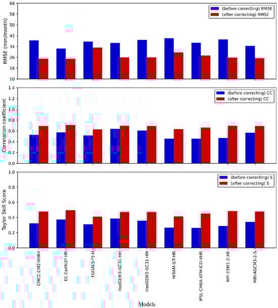
Figure 3.
Comparison of RMSE, CC, and S of nine models before and after bias correction using QM method.
Figure 4 illustrates the spatial distribution of the RMSE for monthly mean precipitation across all models. Notably, the RMSE values are highest in the SC region, which experiences greater rainfall, while the western and northern regions, characterized by lower precipitation levels, exhibit smallest values. This indicates that the capabilities of the models are different under different precipitation conditions. Secondly, throughout the entire western and northern regions, the RMSE values for models (c), (f), and (g) are higher than the other five models. This indicates that the prediction accuracy of these three models is notably lower in these areas. Furthermore, in Xinjiang, although all models indicate low precipitation levels, the NC region exhibits a higher RMSE compared to other areas, ranging from approximately 20 to 30 mm/month. This phenomenon may be linked to the region’s unique climate characteristics or data uncertainties. Across all models, the RMSE values in Southern Tibet are consistently the highest within the entire region. Considering all regions, the RMSE values for models (a), (b), (d), (e), (h), and (i) are comparatively lower among the nine models. Specifically, models (b), (e), (h), and (i) demonstrate superior performance in the SC region, which receives higher rainfall, while models (a) and (d) achieve the best results in the WNW, ENW and TP regions, where precipitation is lower. Overall, the RMSE of the models exhibits varying performance across different regions, which is affected by the variations in precipitation.
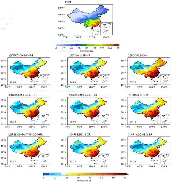
Figure 4.
RMSE of the mean monthly precipitation from the nine models for the 30-year period spanning 1985 to 2014. (The numbers in the lower left corner represent the mean RMSE of the model).
Table 2 presents the RMSE, CC, and S for all models after the QM correction. The RMSE for most models is approximately 25 mm/month, with the exceptions being FGOALS-f3-H at 33.27 mm/month and HiRAM-SIT-HR at 29.73 mm/month. The CCs are predominantly clustered around 0.65, ranging from a minimum of 0.63 to a maximum of 0.71. The S is similarly distributed around 0.45, with values ranging from a minimum of 0.41 to a maximum of 0.50. It is evident that the statistical indicators (RMSE, CC, and S) for the six models—CMCC-CM2-VHR4, EC-Earth3P-HR, HadGEM3-GC31-HH, HadGEM3-GC31-HM, MPI-ESM1-2-XR, and MRI-AGCM3-2-S—rank in the top six. Specifically, these models have RMSE values below 27 mm/month, CC exceeding 0.67, and S higher than 0.46.
Table 2.
RMSE, CC, and S of nine models after bias correction.
To better demonstrate the three statistical indices for the models, their rankings are shown in Figure 5. In the figure, a smaller RMSE corresponds to a higher ranking, while a larger CC and a larger S also indicate a higher ranking. It is found that EC-Earth3P-HR ranks first across all three indicators, while FGOALS-f3-H ranks last. It is observed that the rankings of the three indicators for each model are basically consistent. Based on Table 2 and Figure 5, we exclude the three models—FGOALS-f3-H, HiRAM-SIT-HR, and IPSL-CM6A-ATM-ICO-VHR—and proceed to select the remaining six models for further analysis.
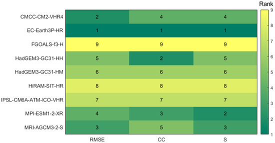
Figure 5.
Ranking charts of RMSE, CC, and S for the nine models (the numbers indicate each model’s rank among all the models).
3.2. BMA for Six Optimal Models
To further reduce the uncertainties of precipitation simulation, this study selects the best-performing models from the nine analyzed models to generate the BMA model. The weights of the six models are calculated as follows: CMCC-CM2-VHR4: 0.1676; EC-Earth3P-HR: 0.1663; HadGEM3-GC31-HH: 0.1661; HadGEM3-GC31-HM: 0.1668; MPI-ESM1-2-XR: 0.1665; and MRI-AGCM3-2-S: 0.1668. Figure 6 illustrates the comparison of the three statistical indicators for the BMA and the six ensemble members. Compared to the single model, the BMA demonstrates lower RMSE but higher CC and S for the period from 1961 to 2014. These findings suggest that the BMA model surpasses the individual models. The RMSE decreased from 24.89 mm/month for the EC-Earth3P-HR, which performs best in six models, to 19.81 mm/month for the BMA model, reflecting an improvement of 20.42%. The corresponding CC increased from 0.71 to 0.82, marking an improvement of 15.7%. Additionally, the corresponding S rose from 0.50 to 0.64, resulting in an enhancement of 29.34%. These improvements highlight the effectiveness of the BMA approach in optimizing model performance.
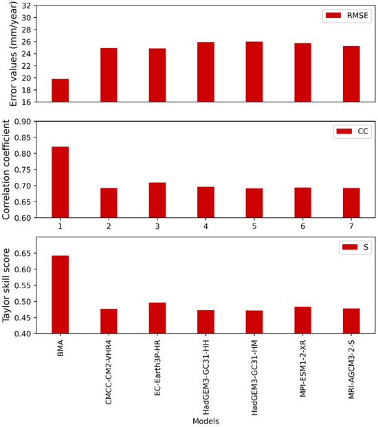
Figure 6.
RMSE, CC, and S for the BMA and six ensemble members.
3.3. Spatiotemporal Variation in BMA Simulations
3.3.1. Evaluation of BMA Simulation
Figure 7 presents the spatial distribution of RMSE for the BMA and the six ensemble members. The BMA model exhibits significantly lower RMSE values in areas of high precipitation, particularly in the SC region, indicating that it outperforms the other six models in these areas. Additionally, in the low-precipitation areas of the WNW region, the BMA model demonstrates a larger extent of lower RMSE values than the other models, highlighting its superior prediction accuracy in these regions. In the NEC region, the improvement effect of the BMA model is also obvious, and it can be seen that the RMSE has been significantly reduced. However, the improvement advantage of the BMA model in the precipitation transition zone—specifically in areas with annual rainfall between 500 and 600 mm—and Southern Tibet is not very pronounced. Overall, the improvement in the BMA model is significant in the NEC, SC, JH, and WNW regions; however, the enhancement in the rainfall transition zone is less pronounced.
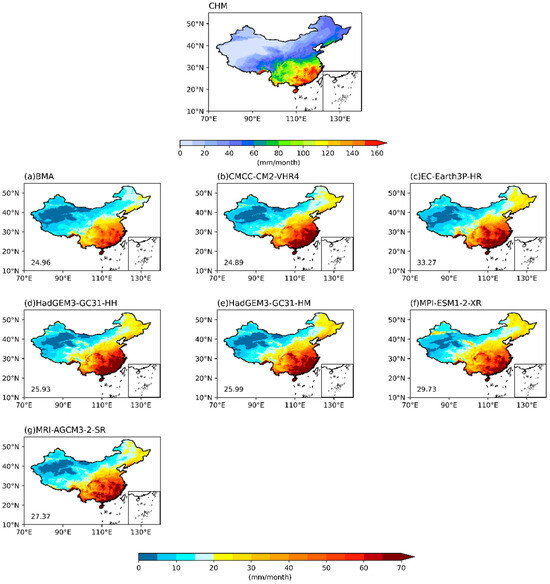
Figure 7.
Distribution of the deviation between the BMA and the ensemble members, along with the annual mean precipitation of the observed data. (The numbers in the lower left corner represent the mean RMSE of the model).
Figure 8 presents a spatial distribution map of annual rainfall trends based on observational data and the BMA model from 1985 to 2014. The precipitation of BMA shows an increasing trend over the past 30 years. Specifically, significant increases can be observed in the NC, ENW, WNW, TP, JH, and SC regions, while decreases have been recorded in the NEC and SWC regions. The most pronounced downward trend in rainfall is observed in Southern Tibet, while the most significant increase is found in the southern part of SC and at the junction of the JH region and the SC. Moreover, the areas with significant increases (p < 0.05) were primarily located in Tibet, Southern Xinjiang, the junction of the SC and JH regions, as well as the southern part of Sichuan (SC). In contrast, the areas with significant decreases (p < 0.05) were mainly found in the southern part of the SC region.
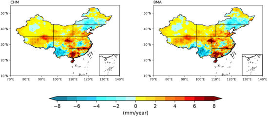
Figure 8.
Spatial distribution of rainfall trends in observational data and BMA from 1985 to 2014.
Overall, the areas identified with increasing and decreasing trends are broadly similar between the two datasets. This consistency is evident not only in the distribution of trends but also in the locations of points identified by the 95% significance tests. However, there are some differences. For instance, the BMA model indicates a more pronounced trend of increasing rainfall in the junction of the JH, as well as in SC, compared to observation.
3.3.2. Seasonal Analysis
Figure 9 displays the spatial variation trends of precipitation across four seasons over a 30-year period for both the BMA model and observational data. The figure reveals that both datasets indicate the most significant trend of change in average monthly precipitation during the summer, while the winter shows the least significant changes. This indicates that summer precipitation often exhibits unstable changes, while winter precipitation remains relatively stable with minimal variation. It can be observed that in summer, the distribution of precipitation increasing and decreasing trends for both the BMA and observational data are quite similar, with most points passing the 95% significance test aligning closely. In other seasons, areas with higher precipitation, such as the SC region, show consistent precipitation change trends between the BMA and observational data. Conversely, in regions with relatively lower precipitation, such as the NEC area, the trends differ. For instance, in autumn, the observational data indicates a decreasing trend in precipitation for the NEC region, while the BMA model shows an upward trend. Thus, it is evident that the simulation of the BMA is better in areas with higher precipitation compared to those with lower precipitation.
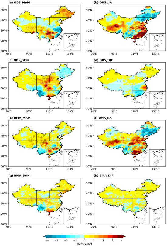
Figure 9.
Spatial variation trends of precipitation in spring (MAM), summer (JJA), autumn (SON), and winter (DJF) from 1985 to 2014 between BMA and observation data.
Figure 10 presents a relative deviation diagram of monthly precipitation between the BMA model and observational data over the past 30 years. Spatially, the WNW and NEC regions demonstrate significant overestimation, while the relative deviation in the SEC region is relatively small. Overall, the BMA model tends to overestimate precipitation relative to the observation data, with this tendency being particularly pronounced in the western region. The BMA model performs better in areas with heavy rainfall, while its performance is slightly worse in areas with light rainfall.
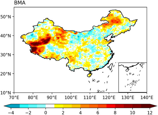
Figure 10.
Relative deviation of precipitation between BMA and observational data over the past 30 years (units: %).
Figure 11 displays a relative deviation analysis for the four seasons over the past 30 years. From a temporal perspective, the overestimation is primarily concentrated in the spring and winter seasons, with nearly all regions exhibiting overestimation. Summer and autumn precipitation is generally underestimated, with autumn exhibiting only a slight overestimation in the rainfall transition zone. While spring and winter are characterized by positive deviations, summer and autumn are predominantly marked by negative deviations. As a result, the overall annual deviation appears to be relatively small.
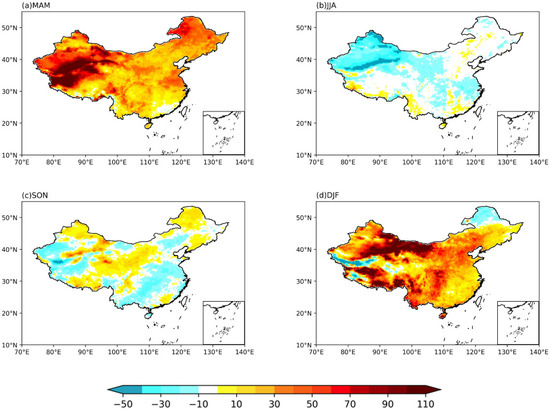
Figure 11.
Relative deviations between BMA and observational data for precipitation in the four seasons over the past 30 years (units: %).
3.3.3. Comparation Between BMA and the Worst Multi-Model Ensemble (WMME) [52]
Figure 12 illustrates the deviations of BMA and WMME in precipitation simulation across various regions during the summer and winter seasons. In China, summer is the season with the most rainfall, and winter is the season with the least rainfall. In summer, both BMA and WMME exhibit negative mean deviations, while in winter, they show positive mean deviations. With the exception of the SC region, the mean deviations of BMA in both winter and summer are better than those of WMME across all other regions, indicating that the BMA model effectively reduces systematic bias. Furthermore, during winter, when precipitation levels are lower, the deviation values are smaller; conversely, in summer, when precipitation is higher, the deviation values are larger.
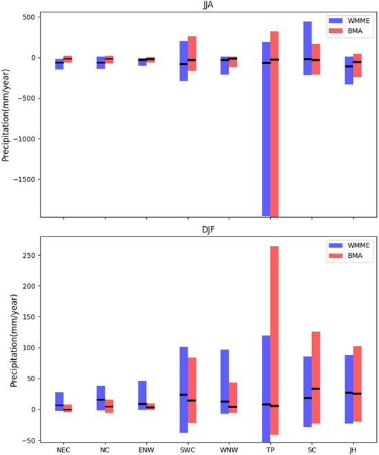
Figure 12.
The mean JJA and DJF precipitation deviations of eight subregions of China simulated by BMA and WMME. (The bars present the range of deviations for each region; the solid black lines show the mean bias for the corresponding region).
A notable phenomenon is that, regardless of seasonal variations, the TP region consistently displays the largest range of deviations. In contrast, the NEC, NC, ENW, and WNW display a relatively small range of deviations. In summer, the deviation range of BMA is smaller than that of WMME, except in the TP area. In winter, BMA also exhibits a smaller deviation range than WMME in most regions, except for the TP, SC, and JH areas. Overall, the deviation range of BMA is smaller than that of WMME across all regions, indicating that BMA has lower uncertainty. Additionally, it has also been found that the simulation differences across various geographical regions in China are relatively significant.
4. Discussion
4.1. Consistency of Assessment Results
The BMA was employed to analyze the 30-year average annual precipitation in the Chinese mainland from 1985 to 2014. The results indicate an upward trend in overall precipitation across the Chinese mainland over the past three decades, with the SC region presenting the most pronounced increase, which aligns with the findings from earlier research. For example, the precipitation of the JH region shows an increasing trend from 1961 to 2014 [53]. The precipitation has been increasing over the past few decades based on CMIP6 models in China [54].
The overestimation and underestimation of some regions in other studies are also consistent with our study. For example, the ensemble of high-resolution CMIP6 models tended to overestimate mean seasonal rainfall in spring while underestimating it in summer [55]. This conclusion aligns with the results of the current studies. When simulating precipitation in China, most high-resolution CMIP6 models tended to underestimate precipitation in the WNW region [56]. Similarly, we also found that BMA underestimated precipitation in certain areas of the WNW. The study found that the highest precipitation levels were recorded in the SC region, while the lowest precipitation was observed in the WNW region, particularly in Xinjiang Province. This aligns with the results from other papers [22]. Overall, these consistent conclusions indicate that our trend analysis and assessment are reasonable.
4.2. Explanation of the Physical Mechanism of Precipitation Differences Simulated by CMIP6 Models
ESMs frequently display specific biases, making it challenging to accurately reproduce historical climate patterns and predict future climate trends. To address this issue, this study employed the QM method for bias correction, aiming to enhance the accuracy of the ESM precipitation simulation. These results indicate that the accuracy of all models’ data has been improved to some extent following bias correction, as evidenced by a reduction in RMSE and improvements in correlation CC and S. However, the discrepancies between simulation and observation remain, with most regions showing an overestimation of precipitation, while some regions exhibit underestimation. This highlights the need for improvements in the physical processes associated with precipitation.
Various studies have provided different explanations for these differences. For example, the mismatch between CMIP model data and observations could be attributed to interdecadal fluctuations in sea surface temperatures that are not caught by multi-model ensembles, as well as an underestimation of aerosol effects in climate models [57]. The underestimation of summer precipitation may result from the models’ failure to accurately simulate the East Asian summer monsoon [22]. In CMIP6 models, precipitation in parts of the TP is generally overestimated, which may be related to the models’ inability to simulate the vertical atmospheric motion of the TP region [14,20,58]. The overestimation of winter precipitation may be ascribed to the CMIP6 models’ inability to catch the connection between the El Niño–Southern Oscillation and the winter monsoon [59]. Additionally, the failure of CMIP6 models to accurately capture China’s complex atmospheric circulation system has led to an overestimation of precipitation [22,60]. CMIP6 models own a limited capacity to accurately simulate the dominant spatial patterns of interannual and interdecadal summer precipitation in Eastern China, resulting in inaccuracies in precipitation simulations [30].
Generally, physical processes are crucial factors influencing the accuracy of ESM simulations of precipitation. Enhancing the model’s capability to accurately catch physical processes is one effective way to improve model performance.
4.3. Uncertainty Analysis
The uncertainty inherent in climate models often poses a significant limitation, particularly at regional scales [61]. However, this uncertainty in global climate models is unavoidable. Internal climate variability can significantly affect climate change and climate predictions, particularly in relation to precipitation [62]. Additionally, uncertainties in model structure, such as significant differences in the physical parameterization schemes among various models, may result in uncertainties in simulations [63,64]. Due to variations in the model’s internal structures, they may respond differently to the same internal climate variability, leading to discrepancies in precipitation simulations [65,66]. When considering scenario uncertainty, the emission scenarios in ESMs and the aerosol forcing within the aerosol–cloud module can significantly impact precipitation simulations and predictions [67]. The sensitivity of the models to changes in greenhouse gas concentrations exhibits uncertainty, with different models potentially responding differently to the same climate change scenarios, leading to different simulations of precipitation [64].
The QM method is a correction technique based on frequency distribution. It calibrates simulated precipitation by developing a transfer function between model data and observed data, thereby reducing uncertainty [68]. BMA reduces the uncertainty of the simulation by calculating the forecast probability density function to achieve a better alignment with the precipitation observations [33]. Meanwhile, BMA employs nonlinear relationships, which allows it to assign different weights to each model and eliminate diagnostic errors, enabling it to outperform individual models [69]. Applying the QM method can help to initially reduce the uncertainty in the model data, selecting the best-performing models can reduce uncertainty among ensemble members, and employing the BMA method can further minimize uncertainty among these best models. Together, these strategies help to ensure that the simulation results align more closely with the observational data.
4.4. Comparison with Low-Resolution Models
Figure 13 shows the values of RMSE, CC, and S for models with both high and low resolutions before bias correction, while Figure 14 presents the corresponding values for these models after bias correction. It is evident that the high-resolution model significantly surpasses the low-resolution model prior to correction, with the RMSE improvement rate ranging from 30.92% to 47.97%. After correction, the high-resolution models continue to outperform the low-resolution model, although the RMSE improvement rate decreases from a range of 30.92% to 47.97% to a range of −3.92% to 5.92%. Furthermore, the results show that the QM method has a significant corrective effect on both models, generating an RMSE improvement rate between 33.53% and 48.84%. Figure 15 and Figure 16 illustrate the performance of the low-resolution and high-resolution models before and after bias correction. A clear improvement can be observed across all three statistical metrics for each model following the bias correction process.
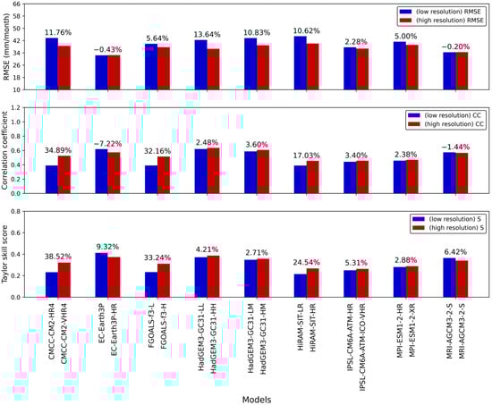
Figure 13.
RMSE, CC, and S for models with both high and low resolutions before bias correction.
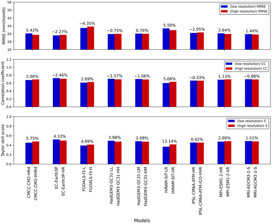
Figure 14.
RMSE, CC, and S for both high-resolution and low-resolution models after bias correction.
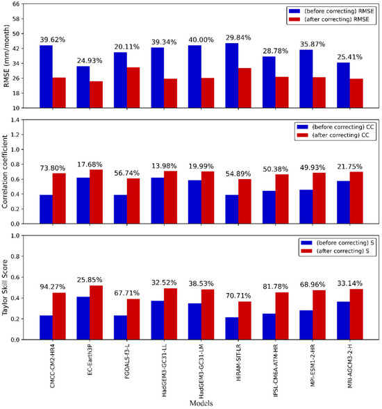
Figure 15.
RMSE, CC, and S for low-resolution models before and after bias correction.
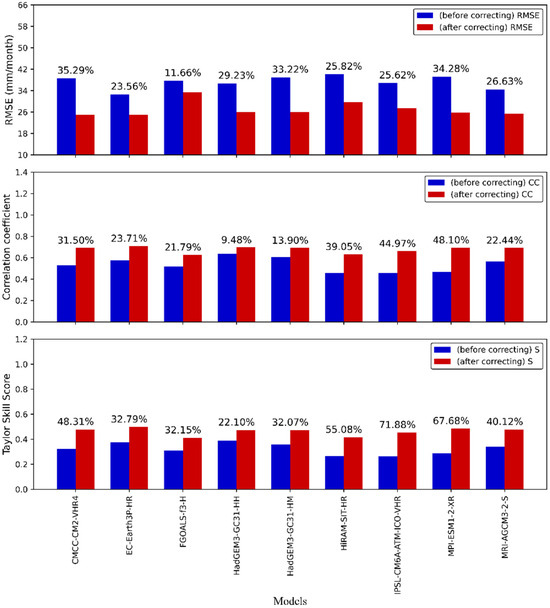
Figure 16.
RMSE, CC, and S for high-resolution models before and after bias correction.
This bias may be attributed to the low resolution of the models, which hampers their ability to accurately replicate atmospheric processes at high altitudes and across complex terrain [70]. Low-resolution models may struggle to accurately simulate local circulation in complex regions, resulting in biased precipitation simulations [53,71,72]. Generally, high-resolution models outperform low-resolution models when simulating precipitation in China. However, some high-resolution models perform slightly worse than low-resolution models after bias correction [30,31,73,74]. And if the model already overestimates precipitation, a higher resolution may lead to an even larger error in the precipitation simulation compared to using a lower resolution [38,75].
The high-resolution models exhibit significantly superior performance compared to the low-resolution models regarding precipitation simulation accuracy, aligning more closely with the actual observations. Therefore, when analyzing the spatiotemporal changes in precipitation across China, employing a high-resolution model proves to be more meaningful than utilizing a low-resolution one. Consequently, this study is based on high-resolution data for our analysis.
5. Conclusions
This study first utilized the QM method to correct the precipitation simulation of nine high-resolution ESMs in CMIP6, and then based on the three evaluation indicators, six best performing models were selected to generate a BMA model. Finally, the spatiotemporal variation characteristics of precipitation across the Chinese mainland from 1985 to 2014 were analyzed by the BMA model. The primary conclusions are as follows:
(1) After the bias correction, the simulation performance of the nine ESMs for precipitation from 1985 to 2014 showed a significant improvement. Compared to the pre-correction results, the RMSE decreased, demonstrating an improvement rate between 11.64% and 35.27%. The CC increased, with an improvement rate ranging from 9.48% to 48.10%. Additionally, the S improved, showing an enhancement rate of 22.10% to 71.88%.
(2) Based on the three evaluation indicators, six best-performing ESMs (CMCC-CM2-VHR4, EC-Earth3P-HR, HadGEM3-GC31-HH, HadGEM3-GC31-HM, MPI-ESM1-2-XR, and MRI-AGCM3-2-S) out of the nine were selected. The BMA method integrated the six best-performing ESMs to obtain a more accurate precipitation simulation result for the Chinese mainland. The results indicate that the BMA model outperforms individual models in terms of precipitation simulation.
(3) The spatial distribution of RMSE for the BMA model showed obvious improvement compared to individual models, particularly in heavy precipitation areas such as SC and JH, as well as in low-precipitation regions like NEC and WNW. However, there was no obvious improvement in the rainfall transition zones. And the areas exhibiting increasing and decreasing precipitation trends in the BMA and observational data were generally similar. This consistency was evident not only in the trend distributions but also in the locations of the points that pass the 95% significance test.
(4) In summer, the trend of BMA precipitation and the locations of the points that passed the 95% significance test are more closely aligned with the observational data relative to other seasons. In addition, the BMA model overestimated precipitation in spring and winter but underestimated it in other seasons.
(5) Both BMA and WMME exhibited a negative mean bias in summer but displayed a positive mean bias in winter. In both summer and winter, the deviation range of BMA is smaller than that of WMME in most regions, except in the TP area during summer and the TP, SC, and JH areas during winter. And the TP region consistently showed the largest bias range in both seasons. Overall, BMA outperformed WMME in terms of mean bias and bias range in both seasons.
(6) In the pre-correction simulation, all high-resolution ESMs exhibited better performance compared to low-resolution ESMs. Similarly, in the corrected simulation with the QM method, all high-resolution models generally outperformed the low-resolution models. Therefore, high-resolution models offered more accurate precipitation simulations than low-resolution models, highlighting the scientific significance of focusing on high-resolution models in this study.
In this study, we employed only the BMA method for data fusion. In future work, we plan to incorporate additional approaches, such as artificial neural networks (ANNs) and convolutional neural networks (CNNs) from the field of machine learning in order to identify the optimal method for precipitation simulation over China. A limitation of the current research is the relatively small number of high-resolution model datasets included due to limited data availability. We hope to integrate more publicly available high-resolution datasets in subsequent studies to achieve more robust and reliable results.
Author Contributions
Conceptualization, H.M. and Z.D.; methodology, H.M.; validation, H.M.; formal analysis, H.M., H.S. and W.Z.; data curation, X.T., X.W. and M.X.; writing—original draft preparation, H.M.; writing—review and editing, H.M. and Z.D.; supervision, Z.D. and Y.L. All authors have read and agreed to the published version of the manuscript.
Funding
This research was funded by the National Key Research and Development Program of China (grant no. 2024YFF0809301) and the National Natural Science Foundation of China (grant no. 42275021).
Institutional Review Board Statement
Not applicable.
Informed Consent Statement
Not applicable.
Data Availability Statement
No new data were created or analyzed in this study.
Acknowledgments
The high-precision gridded precipitation datasets can be obtained at https://doi.org/10.11888/Atmos.tpdc.300523. CMIP6 high-resolution datasets can be found at https://data.ceda.ac.uk/badc/cmip6/data/CMIP6/HighResMIP (accessed on 9 July 2024) and low-resolution datasets can be found at https://aims2.llnl.gov/search/ (accessed on 18 July 2024).
Conflicts of Interest
The authors declare no conflicts of interest.
References
- Zhou, L.; Jiang, Z.H. Future changes in precipitation over Hunan Province based on CMIP5 simulations using the statistical downscaling method of transform cumulative distribution function. Acta Meteorol. Sin. 2017, 75, 223–235. [Google Scholar]
- Han, H.; Zhang, J.; Ma, G.; Zhang, X.; Bai, Y. Advances on impact of climate change on ecosystem services. J. Nanjing Forest. Univ. 2018, 42, 184. [Google Scholar]
- Hou, A.Y.; Kakar, R.K.; Neeck, S.; Azarbarzin, A.A.; Kummerow, C.D.; Kojima, M.; Iguchi, T. The global precipitation measurement mission. Bull. Am. Meteor. Soc. 2014, 95, 701–722. [Google Scholar] [CrossRef]
- Sun, Q.; Miao, C.; Duan, Q.; Ashouri, H.; Sorooshian, S.; Hsu, K.L. A review of global precipitation data sets: Data sources, estimation, and intercomparisons. Rev. Geophys. 2018, 56, 79–107. [Google Scholar] [CrossRef]
- Martens, B.; Cabus, P.; De Jongh, I.; Verhoest, N.E.C. Merging weather radar observations with ground-based measurements of rainfall using an adaptive multiquadric surface fitting algorithm. J. Hydrol. 2013, 500, 84–96. [Google Scholar] [CrossRef]
- Jahanshahi, A.; Roshun, S.H.; Booij, M.J. Comparison of satellite-based and reanalysis precipitation products for hydrological modeling over a data-scarce region. Clim. Dyn. 2024, 62, 3505–3537. [Google Scholar] [CrossRef]
- Huffman, G.J.; Adler, R.F.; Bolvin, D.T.; Gu, G. Improving the global precipitation record: GPCP version 2.1. Geophys. Res. Lett. 2009, 36, L17808. [Google Scholar] [CrossRef]
- Kidd, C. Satellite rainfall climatology: A review. Int. J. Climatol. 2001, 21, 1041–1066. [Google Scholar]
- Ougahi, J.H.; Mahmood, S.A. Evaluation of satellite-based and reanalysis precipitation datasets by hydrologic simulation in the Chenab river basin. J. Water Clim. Change 2022, 13, 1563–1582. [Google Scholar] [CrossRef]
- Wang, A.; Zeng, X. Evaluation of multireanalysis products with in situ observations over the Tibetan Plateau. J. Geophys. Res. 2012, 117, D05102. [Google Scholar] [CrossRef]
- Huang, J.; Zhai, J.; Jiang, T.; Wang, Y.; Li, X.; Wang, R.; Fischer, T. Analysis of future drought characteristics in China using the regional climate model CCLM. Clim. Dyn. 2018, 50, 507–525. [Google Scholar] [CrossRef]
- Zhao, M.; Su, B.; Jiang, T.; Wang, A.; Tao, H. Simulation and projection of precipitation in the upper Yellow River Basin by CMIP6 multi-model ensemble. Plateau Meteorol. 2021, 40, 547–558. [Google Scholar]
- Tu, K.; Yan, Z.; Zhang, X.; Dong, W. Simulation of precipitation in monsoon regions of China by CMIP3 models. Atmos. Ocean. Sci. Lett. 2009, 2, 194–200. [Google Scholar]
- Sun, Q.; Miao, C.; Duan, Q. Projected changes in temperature and precipitation in ten river basins over China in 21st century. Int. J. Climatol. 2015, 35, 1125–1141. [Google Scholar] [CrossRef]
- Meehl, G.A.; Covey, C.; Delworth, T.; Latif, M.; McAvaney, B.; Mitchell, J.F.; Taylor, K.E. The WCRP CMIP3 multimodel dataset: A new era in climate change research. Bull. Am. Meteorol. Soc. 2007, 88, 1383–1394. [Google Scholar] [CrossRef]
- Tao, H.; Gemmer, M.; Jiang, J.; Lai, X.; Zhang, Z. Assessment of CMIP3 climate models and projected changes of precipitation and temperature in the Yangtze River Basin, China. Clim. Change 2012, 111, 737–751. [Google Scholar] [CrossRef]
- Miao, C.; Duan, Q.; Yang, L.; Borthwick, A.G. On the applicability of temperature and precipitation data from CMIP3 for China. PLoS ONE 2012, 7, e44659. [Google Scholar] [CrossRef]
- Gao, C.; Su, B.; Krysanova, V.; Zha, Q.; Chen, C.; Luo, G.; Jiang, T. A 439-year simulated daily discharge dataset (1861–2299) for the upper Yangtze River, China. Earth Syst. Sci. 2020, 12, 387–402. [Google Scholar] [CrossRef]
- Yuan, W. Diurnal cycles of precipitation over subtropical China in IPCC AR5 AMIP simulations. Adv. Atmos. Sci. 2013, 30, 1679–1694. [Google Scholar] [CrossRef]
- Salunke, P.; Jain, S.; Mishra, S.K. Performance of the CMIP5 models in the simulation of the Himalaya-Tibetan Plateau monsoon. Theor. Appl. Climatol. 2019, 137, 909–928. [Google Scholar] [CrossRef]
- Ou, T.; Chen, D.; Linderholm, H.W.; Jeong, J.H. Evaluation of global climate models in simulating extreme precipitation in China. Tellus A 2013, 65, 19799. [Google Scholar] [CrossRef]
- Chen, L.; Frauenfeld, O.W. A comprehensive evaluation of precipitation simulations over China based on CMIP5 multimodel ensemble projections. J. Geophys. Res. Atmos. 2014, 119, 5767–5786. [Google Scholar] [CrossRef]
- Santer, B.D.; Fyfe, J.C.; Pallotta, G.; Flato, G.M.; Meehl, G.A.; England, M.H.; Zou, C.Z. Causes of differences in model and satellite tropospheric warming rates. Nat. Geosci. 2017, 10, 478–485. [Google Scholar] [CrossRef]
- Wei, K.; Xu, T.; Du, Z.; Gong, H.; Xie, B. How well do the current state-of-the-art CMIP5 models characterise the climatology of the East Asian winter monsoon? Clim. Dyn. 2014, 43, 1241–1255. [Google Scholar] [CrossRef]
- Stouffer, R.J.; Eyring, V.; Meehl, G.A.; Bony, S.; Senior, C.; Stevens, B.; Taylor, K.E. CMIP5 scientific gaps and recommendations for CMIP6. Bull. Am. Meteorol. Soc. 2017, 98, 95–105. [Google Scholar] [CrossRef]
- Eyring, V.; Cox, P.M.; Flato, G.M.; Gleckler, P.J.; Abramowitz, G.; Caldwell, P.; Williamson, M.S. Taking climate model evaluation to the next level. Nat. Clim. Change 2019, 9, 102–110. [Google Scholar] [CrossRef]
- Taylor, K.E.; Stouffer, R.J.; Meehl, G.A. An overview of CMIP5 and the experiment design. Bull. Am. Meteorol. Soc. 2012, 93, 485–498. [Google Scholar] [CrossRef]
- Haarsma, R.; Acosta, M.; Bakhshi, R.; Bretonnière, P.A.B.; Caron, L.P.; Castrillo, M.; Wyser, K. HighResMIP versions of EC-Earth: EC-Earth3P and EC-Earth3P-HR. Description, model performance, data handling and validation. Geosci. Model Dev. 2020, 13, 3507–3527. [Google Scholar] [CrossRef]
- Song, F.; Zhou, T. Interannual variability of East Asian summer monsoon simulated by CMIP3 and CMIP5 AGCMs: Skill dependence on Indian Ocean–western Pacific anticyclone teleconnection. J. Clim. 2014, 27, 1679–1697. [Google Scholar] [CrossRef]
- Xin, X.; Wu, T.; Jie, W.; Zhang, J. Impact of higher resolution on precipitation over China in CMIP6 HighResMIP models. Atmosphere 2021, 12, 762. [Google Scholar] [CrossRef]
- Wu, Y.; Zhong, P.A.; Xu, B.; Zhu, F.; Fu, J. Evaluation of global climate model on performances of precipitation simulation and prediction in the Huaihe River basin. Theor. Appl. Clim. 2018, 133, 191–204. [Google Scholar]
- Feng, J.; Lee, D.K.; Fu, C.; Tang, J.; Sato, Y.; Kato, H.; Mabuchi, K. Comparison of four ensemble methods combining regional climate simulations over Asia. Meteorol. Atmos. Phys. 2011, 111, 41–53. [Google Scholar]
- Hu, Y.; Xu, Y.; Li, J.; Han, Z. Evaluation on the performance of CMIP6 global climate models with different horizontal resolution in simulating the precipitation over China. Adv. Clim. Change Res. 2021, 17, 730. [Google Scholar]
- He, L.; Cleverly, J.; Wang, B.; Jin, N.; Mi, C.; Liu, D.L.; Yu, Q. Multi-model ensemble projections of future extreme heat stress on rice across southern China. Theor. Appl. Clim. 2018, 133, 1107–1118. [Google Scholar]
- Jia, B.; Cai, X.; Zhao, F.; Liu, J.; Chen, S.; Luo, X.; Xu, J. Potential future changes of terrestrial water storage based on climate projections by ensemble model simulations. Adv. Water. Resour. 2020, 142, 103635. [Google Scholar]
- Yao, Y.; Liang, S.; Li, X.; Hong, Y.; Fisher, J.B.; Zhang, N.; Feng, F. Bayesian multimodel estimation of global terrestrial latent heat flux from eddy covariance, meteorological, and satellite observations. J. Geophys. Res. Atmos. 2014, 119, 4521–4545. [Google Scholar] [CrossRef]
- Hoeting, J.A.; Madigan, D.; Raftery, A.E.; Volinsky, C.T. Bayesian model averaging: A tutorial (with comments by M. Clyde, David Draper and EI George, and a rejoinder by the authors. Stat. Sci. 1999, 14, 382–417. [Google Scholar]
- Zhou, T.J.; Li, Z. Simulation of the East Asian summer monsoon using a variable resolution atmospheric GCM. Clim. Dyn. 2002, 19, 167–180. [Google Scholar] [CrossRef]
- Shi, X.; Xu, X. Regional characteristics of the interdecadal turning of winter/summer climate modes in Chinese mainland. Chin. Sci. Bull. 2007, 52, 101–112. [Google Scholar] [CrossRef]
- Wu, J.; Gao, X. A gridded daily observation dataset over China region and comparison with the other datasets. Chin. J. Geophys. 2013, 56, 1102–1111. [Google Scholar]
- Han, J.; Miao, C.; Gou, J.; Zheng, H.; Zhang, Q.; Guo, X. A new daily gridded precipitation dataset for the Chinese mainland based on gauge observations. Earth Syst. Sci. Data 2023, 15, 3147–3161. [Google Scholar] [CrossRef]
- Cherchi, A.; Fogli, P.G.; Lovato, T.; Peano, D.; Iovino, D.; Gualdi, S.; Navarra, A. Global mean climate and main patterns of variability in the CMCC-CM2 coupled model. J. Adv. Model. Earth Syst. 2019, 11, 185–209. [Google Scholar]
- An, B.; Yu, Y.; Bao, Q.; He, B.; Li, J.; Luan, Y.; Zheng, W. CAS FGOALS-f3-H dataset for the high-resolution model intercomparison project (HighResMIP) tier 2. Adv. Atmos. Sci. 2022, 39, 1873–1884. [Google Scholar] [CrossRef]
- Roberts, M.J.; Baker, A.; Blockley, E.W.; Calvert, D.; Coward, A.; Hewitt, H.T.; Vidale, P.L. Description of the resolution hierarchy of the global coupled HadGEM3-GC3. 1 model as used in CMIP6 HighResMIP experiments. Geosci. Model Dev. 2019, 12, 4999–5028. [Google Scholar] [CrossRef]
- Eman, K.; Chung, E.S.; Ayugi, B.O. Investigating the skills of HighResMIP in capturing historical and future mean precipitation shifts over Pakistan. Int. J. Climatol. 2024, 44, 3888–3911. [Google Scholar] [CrossRef]
- Boucher, O.; Servonnat, J.; Albright, A.L.; Aumont, O.; Balkanski, Y.; Bastrikov, V.; Vuichard, N. Presentation and evaluation of the IPSL-CM6A-LR climate model. J. Adv. Model. Earth Syst. 2020, 12, e2019MS002010. [Google Scholar]
- Gutjahr, O.; Putrasahan, D.; Lohmann, K.; Jungclaus, J.H.; von Storch, J.S.; Brüggemann, N.; Stössel, A. Max planck institute earth system model (MPI-ESM1.2) for the high-resolution model intercomparison project (HighResMIP). Geosci. Model Dev. 2019, 12, 3241–3281. [Google Scholar] [CrossRef]
- Mizuta, R.; Yoshimura, H.; Murakami, H.; Matsueda, M.; Endo, H.; Ose, T.; Kitoh, A. Climate simulations using MRI-AGCM3. 2 with 20-km grid. J. Meteorol. Soc. Japan 2012, 90, 233–258. [Google Scholar]
- Maraun, D.; Wetterhall, F.; Ireson, A.M.; Chandler, R.E.; Kendon, E.J.; Widmann, M.; Thiele-Eich, I. Precipitation downscaling under climate change: Recent developments to bridge the gap between dynamical models and the end user. Rev. Geophys. 2010, 48, RG3003. [Google Scholar] [CrossRef]
- Tong, Y.; Gao, X.J.; Han, Z.Y.; Xu, Y. Correction of Daily Precipitation Simulation Errors over China Based on the RegCM4 Model. Chin. J. Atmos Sci. 2017, 41, 1156–1166. [Google Scholar]
- Raftery, A.E.; Gneiting, T.; Balabdaoui, F.; Polakowski, M. Using Bayesian model averaging to calibrate forecast ensembles. Mon. Weather Rev. 2005, 133, 1155–1174. [Google Scholar] [CrossRef]
- Yang, X.; Zhou, B.; Xu, Y.; Han, Z. CMIP6 evaluation and projection of temperature and precipitation over China. Adv. Atmos. Sci. 2021, 38, 817–830. [Google Scholar] [CrossRef]
- Duan, Q.; Phillips, T.J. Bayesian estimation of local signal and noise in multimodel simulations of climate change. J. Geophys. Res. 2010, 115, D18123. [Google Scholar] [CrossRef]
- Xing, L.; Huang, L.; Chi, G.; Yang, L.; Li, C.; Hou, X. A dynamic study of a karst spring based on wavelet analysis and the Mann-Kendall Trend Test. Water 2018, 10, 698. [Google Scholar] [CrossRef]
- Mann, H.B. Nonparametric tests against trend. Econometrica 1945, 13, 245–259. [Google Scholar] [CrossRef]
- Jia, Q.; Jia, H.; Li, Y.; Yin, D. Applicability of CMIP5 and CMIP6 models in China: Reproducibility of historical simulation and uncertainty of future projection. J. Clim. 2023, 36, 5809–5824. [Google Scholar] [CrossRef]
- Tian, J.; Zhang, Z.; Fu, Y.; Tao, H.; Zhu, B.; Yang, L. Does CMIP6 inspire more confidence in projecting precipitation over China? Int. J. Climatol. 2023, 43, 4965–4986. [Google Scholar] [CrossRef]
- Yi, P.; Chen, G.; Tang, X. Present and future climate of the Yangtze River Delta region: Analysis of the CMIP6 HighResMIP simulations. Theor. Appl. Climatol. 2024, 155, 8909–8921. [Google Scholar] [CrossRef]
- Li, Z.; Chen, W.; Chen, S.; Sun, Y.; Qian, D. Uncertainty of central China summer precipitation and related natural internal variability under global warming of 1 to 3 °C. Int. J. Climatol. 2021, 41, 6640–6653. [Google Scholar] [CrossRef]
- Biasutti, M. Forced Sahel rainfall trends in the CMIP5 archive. J. Geophys. Res. Atmos. 2013, 118, 1613–1623. [Google Scholar] [CrossRef]
- Wu, C.H.; Freychet, N.; Chen, C.A.; Hsu, H.H. East Asian presummer precipitation in the CMIP5 at high versus low horizontal resolution. Int. J. Climatol. 2017, 37, 4158–4170. [Google Scholar] [CrossRef]
- Jiang, D.; Hu, D.; Tian, Z.; Lang, X. Differences between CMIP6 and CMIP5 models in simulating climate over China and the East Asian monsoon. Adv. Atmos. Sci. 2020, 37, 1102–1118. [Google Scholar]
- Li, Y.; Yan, D.; Peng, H.; Xiao, S. Evaluation of precipitation in CMIP6 over the Yangtze River Basin. Atmos. Res. 2021, 253, 105406. [Google Scholar] [CrossRef]
- Katiraie-Boroujerdy, P.S.; Akbari Asanjan, A.; Chavoshian, A.; Hsu, K.L.; Sorooshian, S. Assessment of seven CMIP5 model precipitation extremes over Iran based on a satellite-based climate data set. Int. J. Climatol. 2019, 39, 3505–3522. [Google Scholar] [CrossRef]
- Hawkins, E.; Sutton, R. The potential to narrow uncertainty in projections of regional precipitation change. Clim. Dyn. 2011, 37, 407–418. [Google Scholar] [CrossRef]
- Piao, J.; Chen, W.; Chen, S. Sources of the internal variability-generated uncertainties in the projection of Northeast Asian summer precipitation. Clim. Dyn. 2021, 56, 1783–1797. [Google Scholar] [CrossRef]
- Huang, D.Q.; Zhu, J.; Zhang, Y.C.; Huang, A.N. Uncertainties on the simulated summer precipitation over Eastern China from the CMIP5 models. J. Geophys. Res. Atmos. 2013, 118, 9035–9047. [Google Scholar] [CrossRef]
- Chen, S.; Wu, R.; Chen, W. Projections of climate changes over mid-high latitudes of Eurasia during boreal spring: Uncertainty due to internal variability. Clim. Dyn. 2019, 53, 6309–6327. [Google Scholar] [CrossRef]
- Lin, L.; Xu, Y.; Wang, Z.; Diao, C.; Dong, W.; Xie, S.-P. Changes in extreme rainfall over India and China attributed to regional aerosol-cloud interaction during the late 20th century rapid industrialization. Geophys. Res. Lett. 2018, 45, 7857–7865. [Google Scholar]
- Latif, M. Uncertainty in climate change projections. J. Geochem. Explor. 2011, 110, 1–7. [Google Scholar] [CrossRef]
- Kokic, P.; Jin, H.; Crimp, S. Improved point scale climate projections using a block bootstrap simulation and quantile matching method. Clim. Dyn. 2013, 41, 853–866. [Google Scholar] [CrossRef]
- Su, F.; Duan, X.; Chen, D.; Hao, Z.; Cuo, L. Evaluation of the global climate models in the CMIP5 over the Tibetan Plateau. J. Clim. 2013, 26, 3187–3208. [Google Scholar] [CrossRef]
- Hagedorn, R.; Doblas-Reyes, F.J.; Palmer, T.N. The rationale behind the success of multi-model ensembles in seasonal forecasting—I. Basic concept. Tellus A 2005, 57, 219–233. [Google Scholar] [CrossRef]
- Chen, H.; Zhou, T.; Neale, R.B.; Wu, X.; Zhang, G.J. Performance of the new NCAR CAM3.5 in East Asian summer monsoon simulations: Sensitivity to modifications of the convection scheme. J. Clim. 2010, 23, 3657–3675. [Google Scholar] [CrossRef]
- Yu, X.; Zhang, L.; Zhou, T.; Zheng, J. Assessing the performance of CMIP6 models in simulating droughts across global drylands. Adv. Atmos. Sci. 2024, 41, 193–208. [Google Scholar] [CrossRef]
Disclaimer/Publisher’s Note: The statements, opinions and data contained in all publications are solely those of the individual author(s) and contributor(s) and not of MDPI and/or the editor(s). MDPI and/or the editor(s) disclaim responsibility for any injury to people or property resulting from any ideas, methods, instructions or products referred to in the content. |
© 2025 by the authors. Licensee MDPI, Basel, Switzerland. This article is an open access article distributed under the terms and conditions of the Creative Commons Attribution (CC BY) license (https://creativecommons.org/licenses/by/4.0/).