Article

Evaporation Duct Height Short-Term Prediction Based on Bayesian Hyperparameter Optimization

1
School of Mathematics and Statistics, Nanjing University of Information Science and Technology, Nanjing 210044, China
2
Center for Applied Mathematics of Jiangsu Province, Nanjing University of Information Science and Technology, Nanjing 210044, China
3
Jiangsu International Joint Laboratory on System Modeling and Data Analysis, Nanjing University of Information Science and Technology, Nanjing 210044, China
4
Beijing Institute of Applied Meteorology, Beijing 100020, China
5
Reading Academy, Nanjing University of Information Science and Technology, Nanjing 210044, China
6
School of Earth and Space Science and Technology, Wuhan University, Wuhan 430072, China
*
Authors to whom correspondence should be addressed.
Atmosphere 2025, 16(10), 1126; https://doi.org/10.3390/atmos16101126
Submission received: 22 July 2025 / Revised: 20 September 2025 / Accepted: 21 September 2025 / Published: 25 September 2025

Abstract

Accurately predicting evaporation duct height (EDH) is a crucial technology for enabling over-the-horizon communication and radar detection at sea. To address the issues of overfitting in neural network training and the low efficiency of manual hyperparameter tuning in conventional evaporation duct height (EDH) prediction, this study proposes the application of Bayesian optimization (BO)-based deep learning techniques to EDH forecasting. Specifically, we developed a novel BO–LSTM hybrid model to enhance the predictive accuracy of EDH. First, based on the CFSv2 reanalysis data from 2011 to 2020, we employed the NPS model to calculate the hourly evaporation duct height (EDH) over the Yongshu Reef region in the South China Sea. Then, the Mann–Kendall (M–K) method and the Augmented Dickey–Fuller (ADF) test were employed to analyze the overall trend and stationarity of the EDH time series in the Yongshu Reef area. The results indicate a significant declining trend in EDH in recent years, and the time series is stationary. This suggests that the data can enhance the convergence speed and prediction stability of neural network models. Finally, the BO–LSTM model was utilized for 24 h short-term forecasting of the EDH time series. The results demonstrate that BO–LSTM can effectively predict EDH values for the next 24 h, with the prediction accuracy gradually decreasing as the forecast horizon extends. Specifically, the 1 h forecast achieves a root mean square error (RMSE) of 0.592 m, a mean absolute error (MAE) of 0.407 m, and a model goodness-of-fit (R2) of 0.961. In contrast, the 24 h forecast shows an RMSE of 2.393 m, MAE of 1.808 m, and R2 of only 0.362. A comparative analysis between BO–LSTM and LSTM reveals that BO–LSTM exhibits marginally superior accuracy over LSTM for 1–15 h forecasts, with its performance advantage becoming increasingly pronounced for longer forecast horizons. This confirms that the Bayesian optimization-based hyperparameter tuning method significantly enhances model prediction accuracy.

1. Introduction

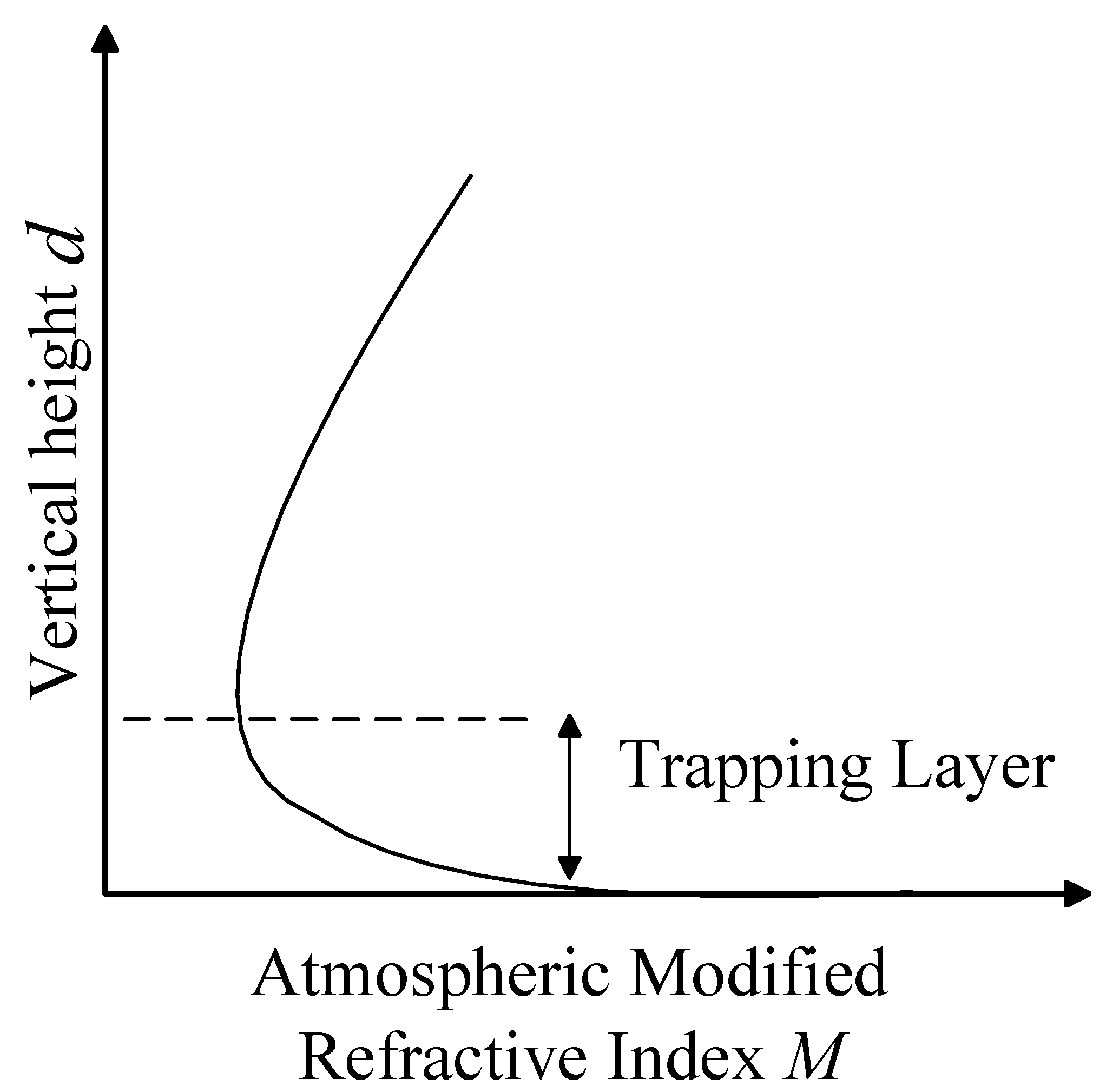
The propertiesof the atmospheric medium significantly alter electromagnetic wave propagation behavior. When abnormal gradients occur in the vertical distribution of atmospheric refractivity, such as temperature inversions or sharp humidity drops, atmospheric ducts can form, trapping electromagnetic waves for propagation within them [1,2,3,4]. The presence of atmospheric ducts allows electromagnetic waves to achieve beyond-line-of-sight propagation with low energy attenuation, which is highly significant for communications, radar detection, and radar blind spot correction [5,6,7]. Evaporation ducts primarily form due to the evaporation of sea surface moisture. An imbalance in the thermal structure of the marine atmospheric boundary layer [8] causes significant water vapor to accumulate near the sea surface through air–sea interactions. Wind transport then diffuses this moisture over a certain region. Above this region lies dry air with low moisture content, while below lies moist air carrying ample water vapor. Since sea surface moisture content is saturated, the moisture content decreases sharply with increasing height above the sea surface [8], creating a gradient in water vapor flux and thus forming an evaporation duct. The EDH can be derived from the modified refractivity profile—the height corresponding to the minimum value of the modified atmospheric refractivity, as shown in Figure 1.
As a major form of marine atmospheric duct, evaporation ducts have an occurrence rate as high as 85% in the South China Sea [9,10,11]. Evaporation ducts alter the propagation path and energy distribution of electromagnetic waves, impacting microwave systems like radar and communications [12]. Therefore, obtaining accurate short-term EDH forecasts is a critical task.
Numerous scholars have proposed evaporation duct models based on similarity theory to calculate modified refractivity profiles within tens of meters above the sea surface. These models commonly utilize hydro-meteorological elements such as atmospheric temperature, humidity, pressure, wind speed, and sea surface temperature at a certain height near the sea surface to compute evaporation duct parameters [13,14]. The Jeske model (1973) [15] used potential refractivity, potential temperature, and potential water vapor pressure instead of atmospheric refractivity, temperature, and water vapor pressure, employing the bulk Richardson number to determine atmospheric stability and the Monin–Obukhov (M–O) similarity length, subsequently solving for EDH. In 1985, Paulus [16] modified the Jeske model using new similarity variable relationships obtained from field experiments, resulting in the Paulus–Jeske (P–J) model. This model requires input variables (atmospheric temperature, relative humidity, wind speed, and sea surface temperature) measured at heights no lower than 6 m. In 1992, Musson-Genon et al. [17] proposed the MGB model, based on M–O similarity theory, using an analytical solution widely applied in numerical weather prediction to compute EDH, simplifying the process for operational use. In 1996, Babin et al. [18] introduced the BYC evaporation duct prediction model, which incorporated air pressure parameters compared to the P–J model, resulting in higher prediction accuracy. In 2000, Frederickson et al. [19] proposed the NPS evaporation duct diagnostic model. This model calculates atmospheric temperature and humidity profiles using M–O similarity theory and derives the vertical pressure distribution using the ideal gas law and hydrostatic equations, offering better stability than other models. In 2016, Yang Shaobo et al. [20] conducted an applicability analysis of the NPS evaporation duct diagnostic model in the South China Sea region. The results showed that the directly measured daily average evaporation duct height was 10.68 m with a duct occurrence probability of 92.5%, while the NPS model’s predicted values yielded a daily average height of 10.25 m and an occurrence probability of 89.4%. The 0.43 m difference in daily average height demonstrates that the NPS model predictions remain largely consistent with actual measurements under stable atmospheric conditions. These duct models differ in criteria for determining EDH and other characteristic quantities. This study uses the Climate Forecast System Reanalysis version 2 (CFSv2) dataset from the National Centers for Environmental Prediction (NCEP), including 2 m air temperature, sea surface temperature, 2 m specific humidity, 10 m U and V wind components, and sea-level pressure data. These data are input into the NPS model to calculate the EDH for the Yongshu Reef area in the South China Sea.
With the booming development of artificial intelligence in the 21st century, machine learning methods have been applied across various fields. Some researchers have utilized machine learning for EDH prediction. Given that the evaporation duct height (EDH) in evaporation duct models can be regarded as a function of atmospheric temperature, sea surface temperature, sea surface pressure, relative humidity, and wind speed, Zhu et al. (2018) [21] collected a large set of point-based meteorological observations and used them as inputs to a multilayer perceptron (MLP) deep learning model, with EDH as the output. Their results showed that the deep neural network approach improved prediction accuracy by at least 80%. Later, Zhao et al. (2020) [22] employed single-station data to drive a backpropagation neural network (BP-NN) for EDH prediction and found that, compared with baseline methods such as the P–J model and support vector regression (SVR), the BP-NN model demonstrated significantly better overall performance as well as strong generalization capability. In 2021, Hong et al. [23] proposed a Seasonal Autoregressive Integrated Moving Average (ARIMA) model, using it to forecast EDH variations in the South China Sea in 2018 with a 95% confidence interval, achieving high prediction accuracy. Zhao et al. [24] constructed an EDH prediction model based on Long Short-Term Memory (LSTM) neural networks. Compared to the BYC, NPS, and XGB models, the LSTM–EDH model showed significantly reduced root mean square error (RMSE) and better fit to measured EDH. Han et al. [12] used EDH data measured in the Yellow Sea, China, between July 2017 and March 2019, comparing LSTM with Support Vector Machine (SVM) and Artificial Neural Network (ANN). The results indicated LSTM errors that were significantly smaller than in other models, highlighting LSTM’s advantage in time series prediction. In 2020, Mai Yanbo [25] employed the Darwinian Evolutionary Algorithm (DEA), Support Vector Machine (SVM), and BP neural network to diagnose the evaporation duct height (EDH). Compared with Support Vector Regression (SVR) and BP neural network, the DEA algorithm not only improved diagnostic accuracy but also provided a nonlinear expression of EDH, facilitating early prediction and mitigation of the impact of evaporation ducts on electromagnetic wave propagation. In the same year, Zhao Wenpeng [26] addressed the limitations of existing EDH diagnostic models by introducing the XGBoost algorithm for the first time in this field, proposing the XGB model. Comparative experiments with the P–J model and multilayer perceptron (MLP) demonstrated that the XGB model exhibited superior accuracy and generalization capability. In 2023, Zhang et al. [27] proposed and validated a Multi-Model Fusion (MMF)-based EDH diagnostic method, utilizing the LIBSVM library for model fusion. The experimental results showed that, compared to the BYC, NPS, NWA, NRL, and LKB models, the MMF model achieved higher diagnostic accuracy and stability under varying meteorological conditions. These studies indicate that point-based modeling can achieve satisfactory accuracy while maintaining computational efficiency, making it particularly suitable for localized applications. In practice, EDH data are spatially sparse, making regional-scale prediction infeasible; therefore, investigating single-point time series prediction is a necessary first step.
Despite the effectiveness of AI methods for time series problems, model hyperparameter settings often rely on empirical trial-and-error from prior studies or practice, greatly reducing model generalization [28]. Bayesian optimization (BO) is a common black-box function optimization method [29] that effectively addresses poor hyperparameter adaptability. Liu Heng et al. (2019) [30] improved a conventional BP neural network using a Bayesian regularization algorithm, overcoming the issue of random initial weights leading to local optima. The analysis showed that the improved BP method’s prediction accuracy was 42.81% higher than the traditional BP method. In 2022, Cui et al. [31] used GPS signal inversion and BO-based deep learning to improve EDH prediction accuracy, achieving a smaller RMSE than traditional methods and demonstrating efficient and accurate duct parameter inversion in noisy environments.
To address the challenges of neural network overfitting during training and low efficiency in manual parameter tuning for traditional evaporation duct height (EDH) prediction, this study proposes the application of Bayesian optimization (BO)-based deep learning technology to EDH forecasting. We construct a novel BO–LSTM hybrid model to enhance prediction accuracy, where the BO algorithm automatically optimizes the hyperparameters of the LSTM network for 24 h EDH prediction. The paper is organized as follows: Section 2.1 describes the EDH calculation. Section 2.2 explains Bayesian optimization theory. Section 2.3 details the LSTM prediction model theory. Section 3 presents the experimental results, including the proposed model’s effectiveness in 24 h EDH prediction and its superiority over the baseline LSTM model. The conclusions are presented in Section 4.

2. Methodology

2.1. Evaporation Duct Height Calculation

The data used in this study originates from the National Centers for Environmental Prediction (NCEP) Climate Forecast System Reanalysis version 2 (CFSv2) dataset. This dataset utilizes the GEOS-5 atmospheric model and GSI data assimilation system, providing global hourly data for atmospheric, land, and oceanic indicators from 2011 to present, representing a further development of the CFSR dataset. The resolution of CFSv2 data is shown in Table 1. To obtain meteorological data for the Yongshu Reef area in the South China Sea, this study extracted the following parameters from the CFSv2 dataset through grid-point slicing: air temperature (2 m), sea surface temperature, specific humidity (2 m), U/V wind components (10 m), and sea-level pressure. The processed data were then input into the NPS model to calculate hourly evaporation duct height (EDH) values for the Yongshu Reef region from 2011 to 2020. The resulting dataset comprises 87,672 data points, providing sufficient volume to support subsequent neural network training.
In the NPS evaporation duct height diagnostic model, the vertical profiles of temperature T and specific humidity q within the surface layer are described by the following equations [32]:
T z = T 0 + θ * k ln z z 0 t Ψ h z L Γ d z ,
q z = q 0 + q * k ln z z 0 t Ψ h z L .
where T z and q z are the air temperature and specific humidity at height z, respectively. L is the Obukhov length. T 0 and q 0 are the sea surface temperature and specific humidity, respectively. θ * and q * are the characteristic scales of potential temperature θ and specific humidity q. k is the Kalman constant, with a value of 0.4. z 0 t is the temperature roughness height. Γ d denotes the dry adiabatic lapse rate, with a value of 9.8 kKM−1.
Ψ h z L represents the stability function. When z L > 0 , Ψ h z L corresponds to stable atmospheric conditions, and in this case [33]
ψ h z L = 1 + 2 3 a z L 3 / 2 + b z L c d e d z L + b c d 1 ,
where the constants are a = 1.0 , b = 2 / 3 , c = 5.0 , and d = 0.35 . When z L < 0 , Ψ h z L corresponds to unstable atmospheric conditions, and in this case [33]
ψ h z L = 2 ln 1 + y 2 , y = 1 16 z L .
Sea surface dimension parameters and roughness parameters were calculated using the COARE 3.0 algorithm. Wind speed and temperature stability correction functions were applied under stable conditions, expressed as
ψ h ( ξ ) = 5 5 4 ln 1 + 3 ξ + ξ 2 · ln 2 ξ + 3 5 2 ξ + 5.24 + 1.93 .
where ξ = z L .
In the NPS model, the pressure profile expression is derived by combining the hydrostatic equation and the ideal gas law:
p z 2 = p z 1 · exp 1.2 · z 1 z 2 T M .
The water vapor pressure profile can be determined using the relationship between specific humidity and vapor pressure:
e = q p ε + 1 ξ q .
where p z 1 and p z 2 represent the pressure at measurement heights z 1 and z 2 . Combining the above equations yields the modified atmospheric refractivity profile. The height corresponding to its minimum value is the evaporation duct height (EDH).

2.2. Bayesian Hyperparameter Optimization

Compared to grid search and random search, hyperparameter optimization algorithms converge faster and are suitable for high-dimensional computationally expensive optimization problems, particularly in finding optimal hyperparameters for machine learning models. Unlike model parameters, hyperparameters must be determined before model training. The optimization objective is formulated as follows [34]:
θ * = arg min θ X f ( θ ) .
where f ( θ ) represents the objective score (e.g., model RMSE on the validation set) to be minimized. f ( θ ) is also referred to as the model loss to be optimized. Note that this loss can be independent of the neural network training loss function. The variables influencing f ( θ ) are the model hyperparameters θ , which in this study include the LSTM’s sequence length, number of units per layer, dropout rate, learning rate, and batch size. Here, θ * represents the optimal hyperparameter combination that minimizes the loss function, while θ can take any value within the predefined domain X of the hyperparameter space.
Bayesian optimization (BO) is a highly effective global optimization algorithm aimed at finding the global optimum. It constructs a probabilistic model (e.g., Gaussian Process) of the objective function, requiring only specification of inputs and outputs without knowledge of internal structure or mathematical properties. It automatically selects the most promising hyperparameters to evaluate, updating the posterior distribution of the objective function until the posterior closely approximates the true distribution [35]. The BO algorithm formula is [36]
p θ D 1 : t = p D 1 : t θ p ( θ ) p D 1 : t .
where θ represents parameters in the objective function or probabilistic surrogate model; D 1 : t denotes the observed dataset of size t; p D 1 : t θ is the likelihood distribution of the observed data given parameter θ ; p ( θ ) is the prior probability distribution of θ ; p D 1 : t is the marginal likelihood of D 1 : t ; p θ D 1 : t is the posterior probability distribution of θ after being updated by the observed data D 1 : t .
The Bayesian optimization framework has two key components: (1) using a probabilistic model as a surrogate for the original expensive-to-evaluate complex objective function; (2) utilizing the posterior information of the surrogate model to construct an active selection strategy, known as the acquisition function. The Tree-structured Parzen Estimator (TPE) algorithm proposed by Bergstra et al. in 2011 [37] is an efficient black-box optimization method that automatically searches for optimal parameters, supports early termination, and offers simplicity and efficiency. It is a Sequential Model-Based Global Optimization (SMBO) algorithm. Compared to Genetic Algorithms (GAs) and Particle Swarm Optimization (PSO), it uses an approximation of the fitness function instead of the true one, reducing evaluation costs [38].
The TPE algorithm uses a Gaussian Process (GP) as the surrogate model to model the objective function f ( θ ) (validation set loss):
f ( θ ) GP μ ( θ ) , k θ , θ i ,
where μ ( θ ) is the mean function (often set to 0), and k θ , θ i is the covariance function (kernel function) measuring the similarity between parameter combinations. Typically, k θ , θ i is the Squared Exponential (RBF) kernel:
k θ , θ i = σ 2 exp θ θ i 2 2 h 2 .
where h is the length-scale controlling smoothness.
The TPE algorithm partitions the observation data D = θ i , f ( θ i ) i = 1 N into two groups:
D g o o d = θ i f ( θ i ) f * D b a d = θ i f ( θ i ) > f * .
where D g o o d , D b a d represent the sets of hyperparameter combinations with the best and worst performance, respectively; f * is the γ % quantile threshold (default γ = 25 ).
TPE uses Kernel Density Estimation (KDE) to fit the distributions of hyperparameters in the good and bad groups:
p θ | g o o d = 1 | D g o o d | θ i D g o o d k θ , θ i p θ | b a d = 1 | D b a d | θ i D b a d k θ , θ i .
The acquisition function determines the next hyperparameter combination to evaluate. It maps from the input space χ , observation space R , and hyperparameter space Θ to the real number space: α : χ × R × Θ R . This function is constructed from the posterior distribution derived from the observed dataset D 1 : t . The next evaluation point x t + 1 is selected by maximizing the acquisition function:
x t + 1 = max x χ α t x ; D 1 : t .
Bergstra et al. [37] used Expected Improvement (EI) as the acquisition function:
EI ( θ ) p ( θ g o o d ) p ( θ b a d ) ,
The optimization objective is
θ n e x t = arg max θ EI ( θ ) .
The physical meaning is as follows: select θ such that its probability of occurrence in the g o o d group is much higher than in the b a d group.

2.3. LSTM Model Construction

Short-term EDH prediction uses observations from the previous period to forecast the next prediction window h. The predicted value at time t + h can be calculated as follows [39]:
x t + h = F h x t , f t 1 ,
where h is the prediction window, x ( t ) is the measured EDH value at the current time, f ( t 1 ) represents historical features of EDH reflecting temporal dependencies, and F h is the nonlinear neural network model.
Long Short-Term Memory (LSTM) is a special type of Recurrent Neural Network (RNN), proposed by Hochreiter and Schmidhuber in 1997 [40]. It primarily addresses the vanishing and exploding gradient problems in traditional RNNs when handling long sequences, enabling better capture of long-term dependencies in time series data.
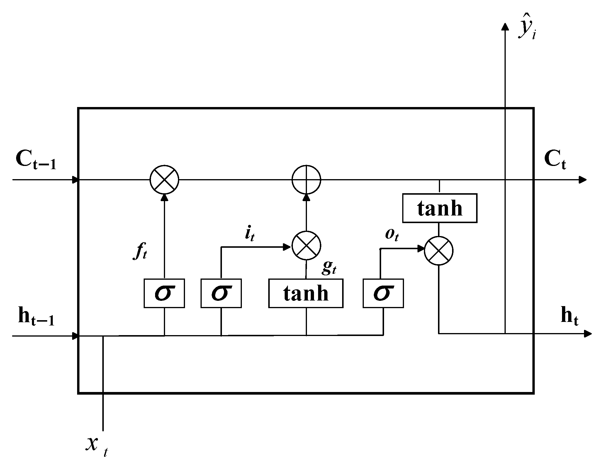
LSTM introduces memory cells and gating mechanisms (gates) to control information flow, deciding what information to retain or discard. The core component is a memory cell (cell state), updated and propagated through three gating mechanisms, as shown in Figure 2.
The specific calculation formulas are as follows [41]:
f t = σ W x f x t + W h f h t 1 + b f ,
g t = t a n h W x g x t + W h g h t 1 + b g ,
i t = σ W x i x t + W h i h t 1 + b i ,
C t = f t · C t 1 + i t · g t ,
o t = σ W x o x t + W h o h t 1 + b o ,
h t = o t t a n h C t ,
y ^ t = W y h h t + b y .
where C t denotes the memory cell state at time t, inheriting from the previous cell and containing partial memory from prior cells; h t represents the hidden state at time t; f t , i t , and o t are the forget gate, input gate, and output gate, respectively; g t is the candidate memory cell; x t and y ^ t are the input and output at time t, respectively; σ ( · ) and t a n h ( · ) represent the Sigmoid activation function and the hyperbolic tangent activation function, respectively.

2.4. Model Evaluation Metrics

To provide a more intuitive demonstration of the model’s predictive accuracy, we adopt root mean square error (RMSE), mean absolute error (MAE), mean squared error (MSE), mean absolute percentage error (MAPE), and the coefficient of determination ( R 2 ) as evaluation metrics. Here, y ^ i is the predicted EDH value, y i is the true EDH value, y ¯ is the mean of true EDH values, and n is the number of predictions.
(1) Root Mean Square Error (RMSE): The square root of the average of the squared differences between predicted and true values. Highly sensitive to prediction error magnitude:
RMSE = 1 n i = 1 n y ^ i y i 2 .
(2) Mean Absolute Error (MAE): The average of the absolute distances between predicted and true values. Avoids error cancellation caused by positive and negative deviations:
MAE = 1 n i = 1 n | y ^ i y i | .
(3) Mean Absolute Percentage Error (MAPE): Measures the relative difference between predicted and true values, expressed as a percentage:
MAPE = 1 n i = 1 n y ^ i y i y i × 100 % .
(4) Coefficient of Determination ( R 2 ): Indicates model fitting performance. Values closer to 1 indicate better predictive performance:
R 2 = 1 i = 1 n y i y ^ i 2 i = 1 n y i y ¯ 2 .
(5) Mean Squared Error (MSE): MSE is a commonly used metric to evaluate the discrepancy between model-predicted values and true values, primarily reflecting the precision and stability of predictions. The calculation formula for MSE is
MSE = 1 n i = 1 n ( y i y ^ i ) 2 .

2.5. Wilcoxon Signed-Rank Test

The Wilcoxon signed-rank test (WSR) is a non-parametric statistical method proposed by Frank Wilcoxon in 1945 [42]. It is mainly used to compare two paired samples (or two treatment conditions of the same sample) to test whether there is a significant difference in their median distributions. Unlike the paired t-test, this method does not rely on the assumption of normality. Instead, it draws inference based on the rank information of the differences. Its basic principle is as follows:
(1) Construct the difference sequence
Given paired data ( x i , y i ) , i = 1 , 2 , , n , calculate the difference:
d i = x i y i .
If d i = 0 , then the sample is discarded, and the remaining number of valid samples is denoted as n .
(2) Rank assignment
Arrange the absolute values of the differences d i in ascending order and assign ranks. In the case of ties, assign the average rank. Denote the rank of the i-th sample as R i .
(3) Sign weighting and rank-sum statistic
According to the signs of the differences, accumulate the ranks separately:
W + = d i > 0 R i ,   W = d i < 0 R i .
The two satisfy the relation
W + + W = n n + 1 2 .
The test statistic is defined as
T = min W + , W .
(4) Testing principle
Under the null hypothesis H 0 , where the median of ( d i ) = 0 , the sequence of differences should be approximately symmetric around zero, and thus the expected values of the positive and negative rank sums ( W + and W ) should be close. If a systematic difference exists (alternative hypothesis H 1 ), one of the rank sums will be significantly larger. In the case of large samples, W + (or W ) approximately follows a normal distribution, and its standardized test statistic is given by
Z = W + n n + 1 4 n n + 1 2 n + 1 24 .
By calculating the Z-value and comparing it with the significance level α , one can determine whether to reject the null hypothesis.

3. Results and Discussion

Based on the evaporation duct height (EDH) calculation method described in Section 2.1, this study derived the hourly EDH time series for the Yongshu Reef region of the South China Sea from 2011 to 2020.

3.1. Overall Trend and Stationarity Analysis of Evaporation Duct Height

In this study, we applied the Mann–Kendall (M–K) nonparametric test to analyze the overall trend of the EDH time series. This method does not rely on the overall data distribution and directly assesses linear trends in the time series. The principle involves using the forward sequence statistic ( U F k ) to detect significant trends and the backward sequence statistic ( U B k ) to detect change points (sudden significant trend shifts). In the M–K test, UFk and UBk are time-varying statistical measures rather than fixed parameter values. Figure 3 displays the M–K statistical curves for EDH (Evaporation Duct Height) hourly data from 2011 to 2020. The red dashed lines represent the critical values of the confidence interval at a significance level of α = 0.05 , with the upper threshold at +1.96 and the lower threshold at −1.96. These lines are used to determine whether the trend changes in the UFk and UBk curves are statistically significant. From the graph, it can be observed that, at hour 15,278 (approximately 2013), the UFk value was −1.985, which exceeded the lower significance threshold (−1.96). From this point onward, the UFk values consistently remained outside the [−1.96, 1.96] confidence interval, indicating a statistically significant decreasing trend in evaporation duct height from 2013 to 2020.
Based on the conclusions drawn from Figure 3, this study employed the Augmented Dickey–Fuller (ADF) test and the Ljung–Box test to examine the stationarity of the hourly EDH data. Table 2 presents the ADF and LB test statistics and corresponding p-values for the EDH hourly data. Table 2 shows that the p-values for the LB test are all less than 0.05, indicating that the time series does not exhibit white noise characteristics and contains extractable information. For the ADF test assessing stationarity, the p-values are also less than 0.05, confirming that the EDH hourly data is stationary. Therefore, using stationary EDH hourly data as input for deep learning models can improve convergence speed and prediction stability.

3.2. EDH Short-Term Prediction Model Based on BO–LSTM

The performance of neural networks heavily depends on the appropriate configuration of various hyperparameters. Key hyperparameters such as time step length (sequence_length), learning rate (learning_rate), number of neurons per layer (units), batch size (batch_size), and dropout ratio require tailored adjustment based on specific dataset characteristics for optimal modeling results. In this study, we innovatively employed the Tree-structured Parzen Estimator (TPE) algorithm based on Bayesian optimization, proposed by Bergstra et al. in 2011 [37], to automatically search for the optimal hyperparameter combination. The core objective of this optimization process is to find the parameter configuration that minimizes the validation set loss function within predefined parameter search spaces. The experimental results of Bergstra et al. [37] show that the TPE algorithm achieves optimal accuracy within 80–200 iterations and significantly outperforms manual and random search methods. Considering both the experimental conclusions of Bergstra et al. [37] and computational costs, we set the number of Bayesian optimization iterations to 100.

3.2.1. LSTM Model Construction

Given that evaporation duct height (EDH) may be influenced by multiple factors and thus exhibits considerable variability and uncertainty, this study focused on modeling and forecasting the hourly EDH data to gain a deeper understanding of its dynamic evolution.
The complete EDH dataset (n = 87,672) was split into three subsets following an 8:1:1 ratio for training, validation, and testing purposes, respectively. Data normalization can significantly enhance the convergence efficiency of gradient descent algorithms, helping the model to find the global optimum faster and potentially improving prediction accuracy. In this study, normalization to the [0, 1] range was applied uniformly to both the training and test sets. This study implemented a tiered data shuffling strategy where training set batches are dynamically shuffled each epoch to eliminate spurious temporal dependencies and enhance model generalization, while the validation set undergoes controlled shuffling during cross-validation to maintain evaluation robustness without compromising temporal integrity, and, crucially, the test set preserves the original chronological ordering throughout all the experiments to prevent data leakage and simulate real-world forecasting conditions. Early Stopping was employed during model training: if the validation loss showed no improvement for 20 consecutive epochs, training was halted to prevent overfitting. The Adam optimizer [43] was chosen for network training to update model weights. The mean squared error (MSE) loss function [44] was used to evaluate training effectiveness.
To validate the effectiveness of LSTM modeling with Bayesian hyperparameter optimization, the LSTM-based evaporation duct height (EDH) prediction model in this study was primarily constructed following the LSTM framework proposed by Han et al. [12]. However, Han et al. [12] only conducted nowcasting for EDH at 30 min, 1 h, and 2 h lead times using a direct multi-step forecasting method, where one model is built for each forecast step (s steps require s models), resulting in low computational efficiency. Therefore, we innovatively conducted short-term (1–24 h) EDH predictions using a direct multi-step forecasting approach, where a single model simultaneously outputs values for multiple future time steps in one forward pass, as opposed to recursive step-by-step prediction. Based on the aforementioned analysis, the parameter configurations of the input layer, hidden layer, and output layer in our BO–LSTM model are detailed in Table 3. The model employs a direct multi-step forecasting mechanism, with its core design featuring 24 output neurons that, respectively, correspond to EDH predictions for each hourly time step over the 24 h forecast horizon. By defining the output layer dimension as (batch_size, 24), the architecture directly maps to EDH values at 24 target time points, thereby effectively circumventing the inherent error accumulation issue in recursive forecasting approaches.

3.2.2. Bayesian Hyperparameter Optimization

During the hyperparameter optimization process, whether using traditional manual tuning or widely applied methods like grid search and random search, reasonable value ranges must be set for each hyperparameter. Similarly, when using the TPE algorithm to automatically search for the optimal hyperparameter combination, the effective search range for each hyperparameter must be predefined. Based on the domain knowledge and preliminary experimental results, this study determined the specific search ranges for each hyperparameter. Table 4 details the initial search ranges for each hyperparameter and the optimal combination obtained after 100 iterations of the optimization algorithm.
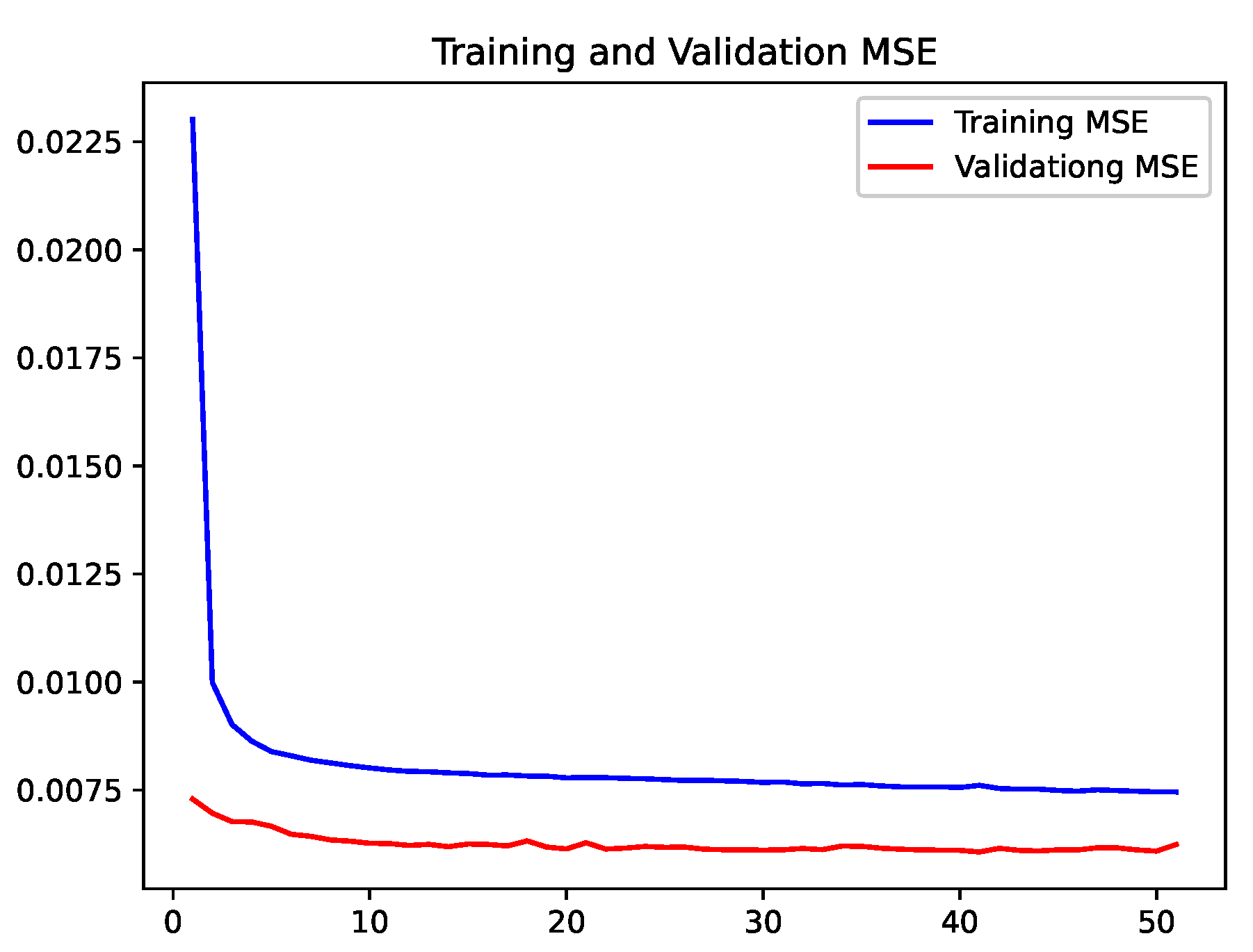
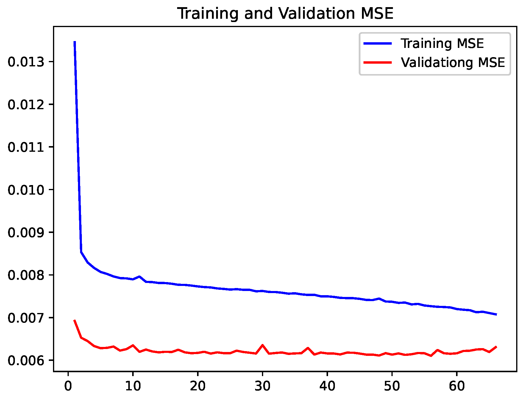
Figure 4 displays the loss function curve under optimal parameter combinations with three hidden layers, where the horizontal axis represents training epochs and the vertical axis denotes MSE values. It can be observed that the training set MSE rapidly converges to around 0.0075 after approximately 10 epochs. The validation set MSE reaches its lowest value of 0.00607 at epoch 41. The validation MSE remains consistently stable at a level slightly lower than the training MSE, indicating that the model trained with Bayesian optimization performs well without overfitting.

3.3. EDH Short-Term Prediction Result Analysis

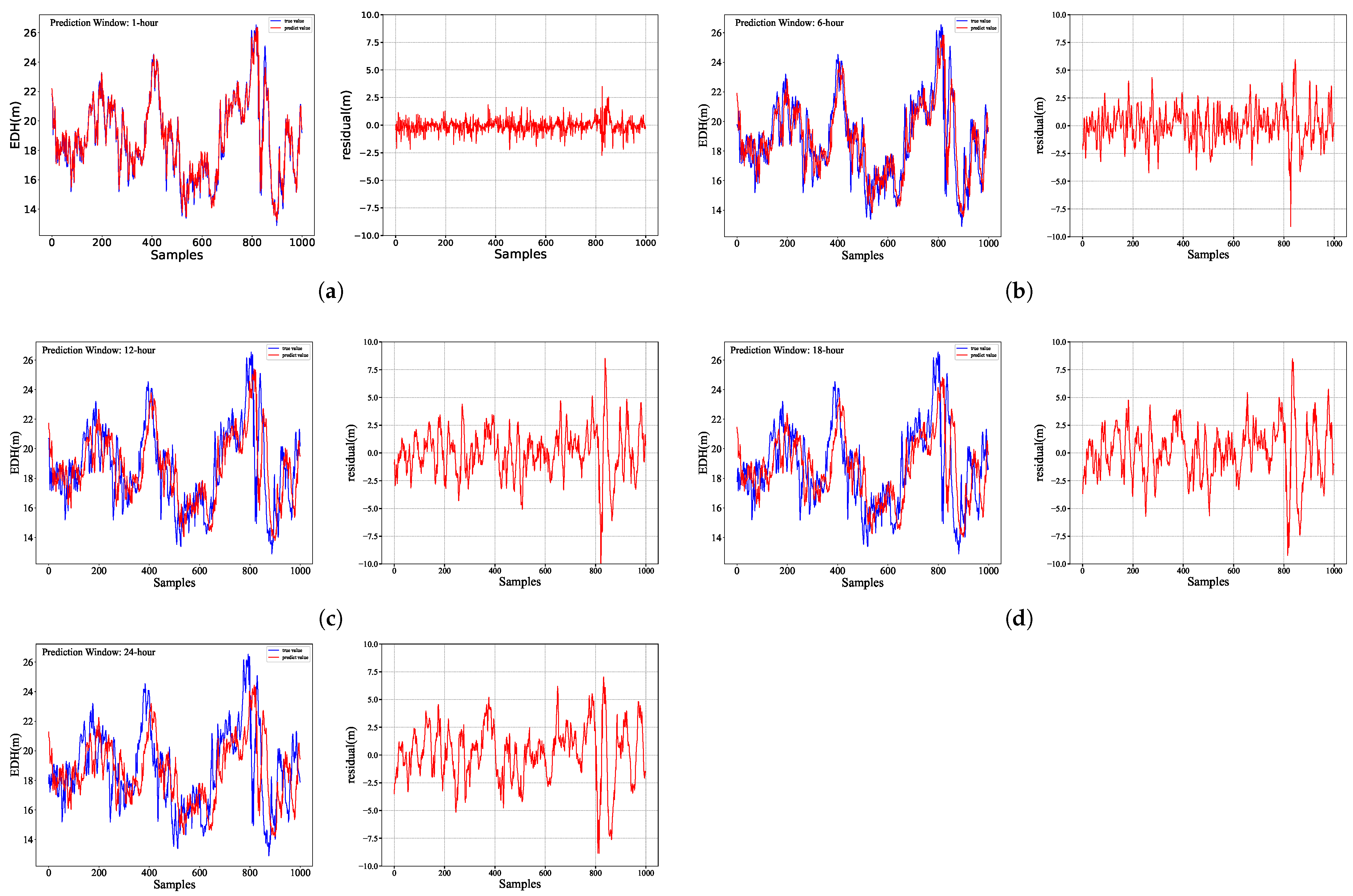
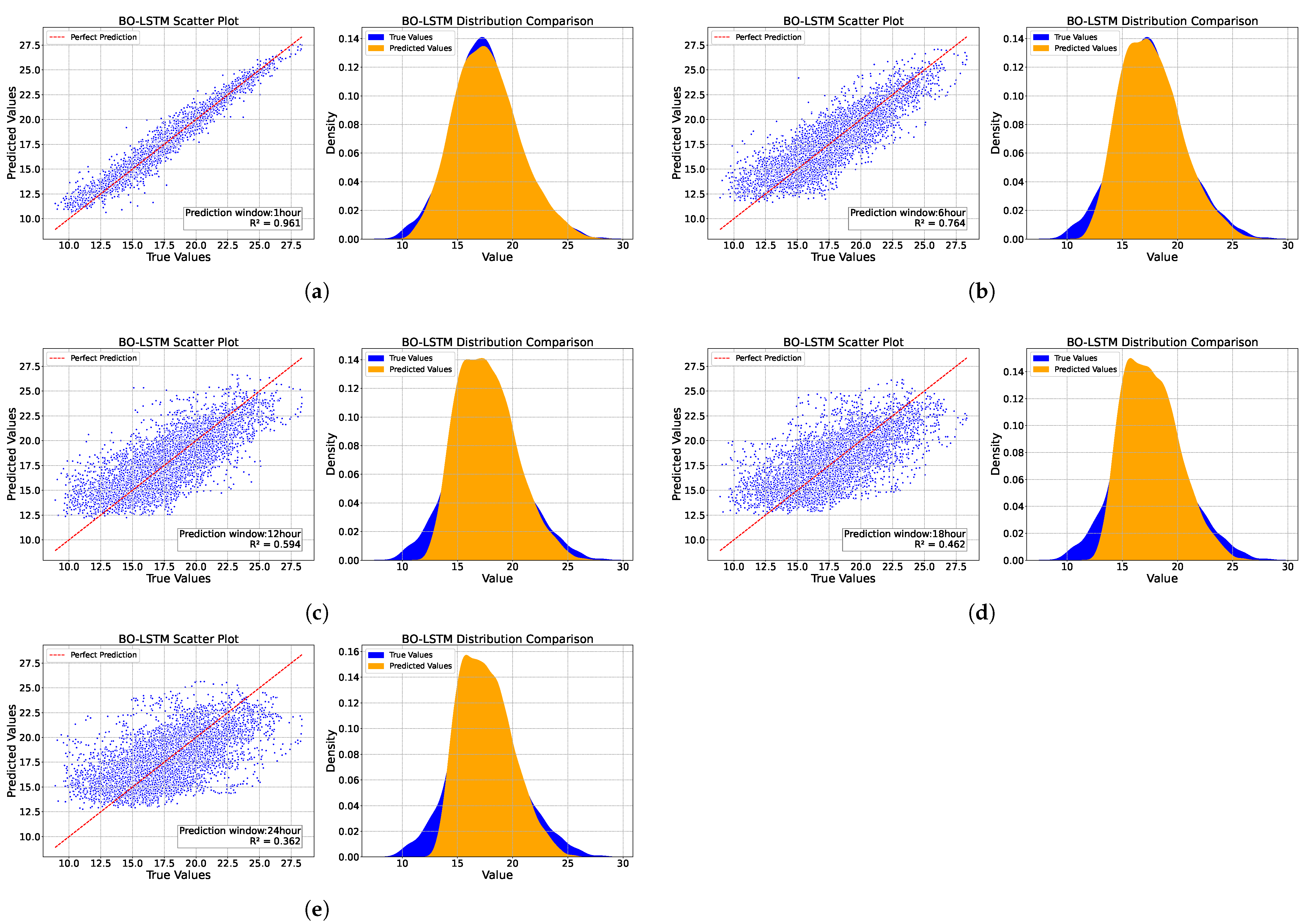
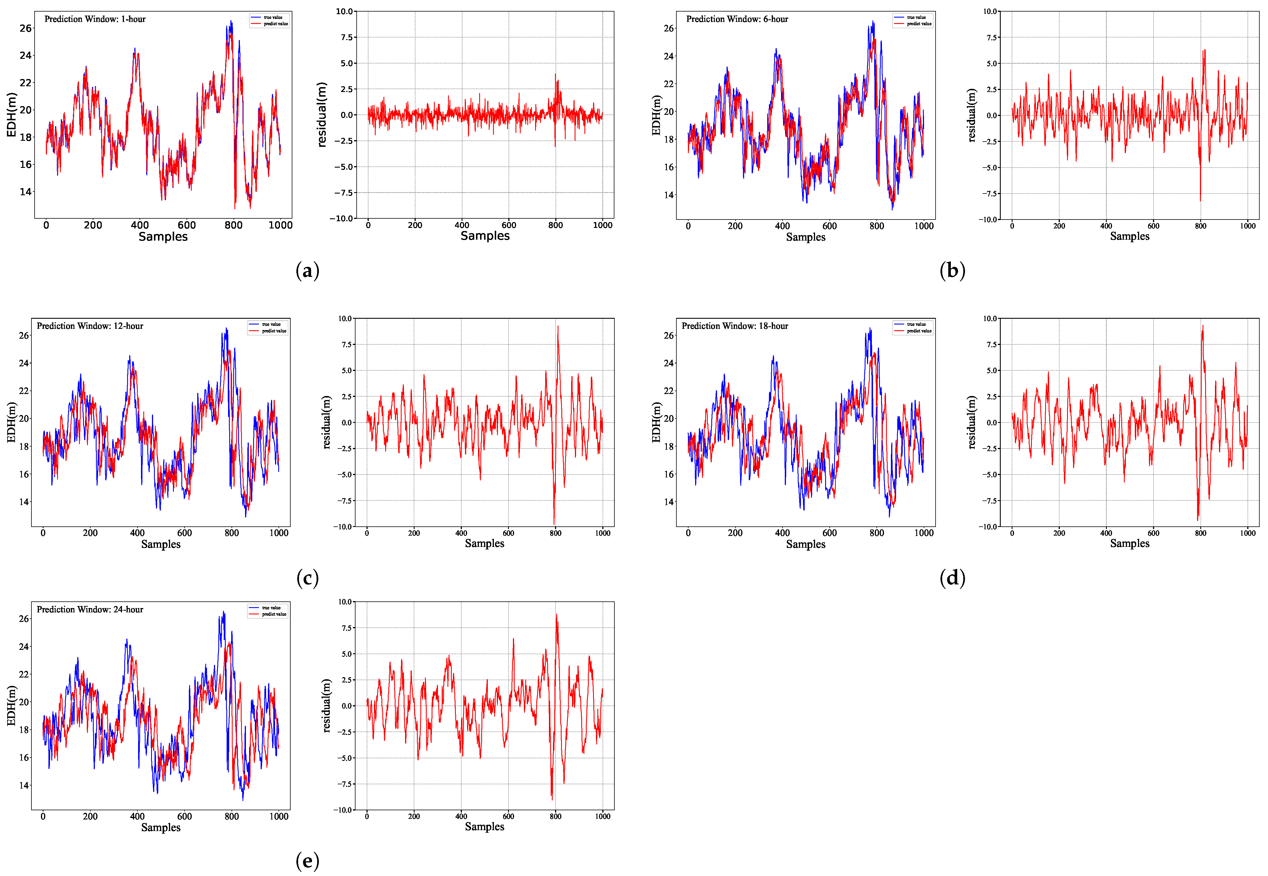
Based on the BO–LSTM model constructed in Section 3.2, we performed a 24 h short-term EDH for the Yongshu Reef area. Figure 5 presents the prediction performance of the BO–LSTM model for a continuous set of 1000 samples in the test set at forecast lead times of 1, 6, 12, 18, and 24 h. The left panel shows the forecast vs. actual values, while the right panel shows the corresponding residuals. It can be seen that the predicted values for 1 h and 6 h lead times closely match the true values. However, as the forecast lead time increases, the discrepancy between the BO–LSTM predictions and the true values becomes significantly larger. To further analyze the increasing error phenomenon in the BO–LSTM model’s forecasts, Figure 6 demonstrates the overall performance of the BO–LSTM model in EDH predictions at 1, 6, 12, 18, and 24 h lead times. As shown in Figure 6, the scatter points of the BO–LSTM model’s 1 h EDH predictions closely cluster around the regression line with the observed values, and their marginal distributions exhibit similar normal distribution shapes, although the predicted values are systematically lower than the actual measurements. As the forecast lead time increases, the scatter points between the predicted and observed EDH values become progressively more dispersed, and the differences between the marginal distributions of the true and predicted values grow more pronounced.
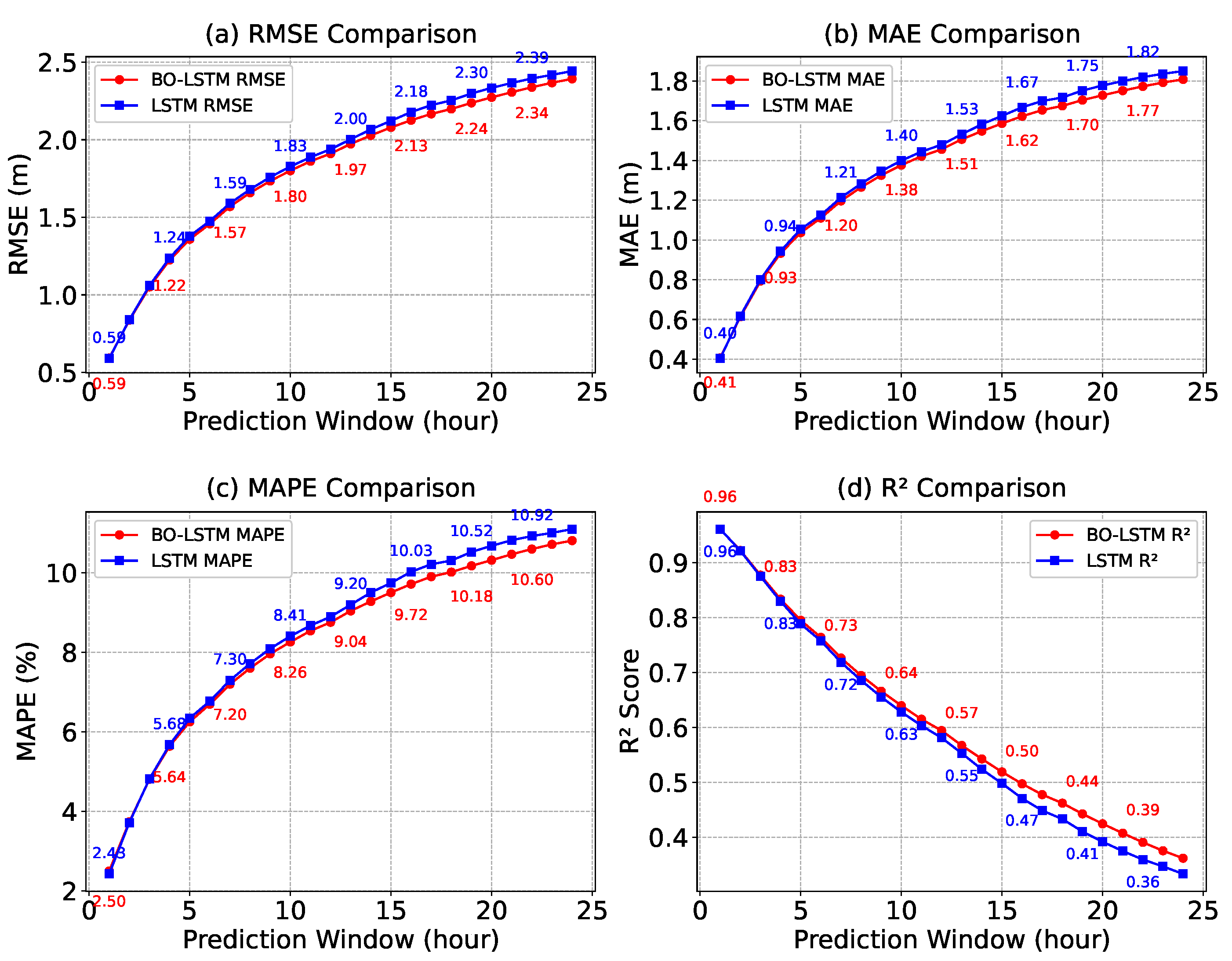
The red line in Figure 7 shows the statistical results of various evaluation metrics for the BO–LSTM 24 h forecast. The results demonstrate that BO–LSTM can effectively predict EDH values for the next 24 h, with the prediction accuracy gradually decreasing as the forecast horizon extends. Specifically, the 1 h forecast achieves a root mean square error (RMSE) of 0.592, a mean absolute error (MAE) of 0.407 m, and a model goodness-of-fit (R2) of 0.961. In contrast, the 24 h forecast shows an RMSE of 2.393, MAE of 1.808 m, and R2 of only 0.362. However, the single-point prediction approach adopted in our study can only provide EDH estimates for specific locations, failing to capture the spatial heterogeneity of its distribution (e.g., horizontal gradients and localized abrupt variations).
To horizontally validate the modeling effectiveness of BO–LSTM, we compared the 1 h and 2 h prediction results of BO–LSTM with those of the LSTM model proposed by Han J et al. [12]. As shown in Table 5, for 1 h predictions, our proposed BO–LSTM model achieved 68.78%, 65.25%, and 83.20% improvements in RMSE, MAE, and MAPE forecasting accuracy, respectively, compared to the model proposed by Han J et al. [12]. For 2 h predictions, the model achieved 68.66%, 64.94%, and 82.92% improvements in RMSE, MAE, and MAPE forecasting accuracy, respectively. These results demonstrate that the method of automatically finding optimal model hyperparameters based on Bayesian optimization can significantly enhance the prediction accuracy of the model.

3.4. Discussion

3.4.1. LSTM Parameter Selection

To validate the effectiveness of the BO–LSTM model, this study constructed a benchmark LSTM model with an identical architecture. During the training of the LSTM model, the Early Stopping technique was equally employed; the training process would terminate if no improvement in validation loss was observed over 20 epochs, thereby preventing model overfitting. In this experiment, manual hyperparameter tuning was adopted. Through multiple experimental trials, we selected seven sets of hyperparameter combinations that demonstrated superior training performance, with their comparative results illustrated in Figure 8. It can be observed that the LSTM model achieves the minimum validation MSE of 0.00610 in Case 4. The optimal hyperparameter combination for the LSTM model at this point is listed in Table 6. The training effect of the LSTM model is shown in Figure 9.
As an example, Figure 10 shows the prediction performance of the LSTM model for the same continuous set of 1000 samples in the test set at forecast lead times of 1, 6, 12, 18, and 24 h. The left panel shows the forecast vs. actual values, and the right panel shows the corresponding residuals. It can be seen that the LSTM-predicted values for 1 h and 6 h lead times also closely match the true values. However, similar to BO–LSTM, the discrepancy between the LSTM predictions and true values becomes increasingly significant as the forecast lead time increases.

3.4.2. Comparative Validation

To further compare the prediction accuracy differences between the BO–LSTM and LSTM models, we conducted statistical analyses of the performance metrics across both models. From Figure 7, it can be observed that the prediction accuracy of the BO–LSTM and LSTM models is comparable for lead times of 1–15 h, with BO–LSTM slightly outperforming LSTM. As the forecast time lengthens, the difference in prediction accuracy between BO–LSTM and LSTM becomes increasingly pronounced. Figure 11 shows the error distribution plots for the BO–LSTM and LSTM models at forecast lead times of 1, 6, 12, 18, and 24 h. It can be seen that, as the forecast time increases, the error distributions of both models become more dispersed, with the LSTM model’s error distribution showing greater dispersion.
To compare the two paired samples, the Wilcoxon signed-rank test (WSR) was applied to statistically assess the differences in prediction accuracy between BO–LSTM and LSTM. The corresponding results are summarized in Table 7.
Table 7 presents the results of the Wilcoxon signed-rank (WSR) test, showing the WSR values and corresponding p-values. The significance of the differences between the model predictions and the control values varies across different forecast lead times. Overall, for most lead times from 1 to 15 h, the p-values are greater than 0.05, indicating that the differences between the model predictions and the control group are not statistically significant and the forecasts are relatively stable. For instance, at hour 2 ( p = 0.806 ), hour 3 ( p = 0.648 ), and hour 11 ( p = 0.762 ), the p-values are well above the significance level, suggesting no statistically significant difference between the BO–LSTM model and the baseline LSTM model. However, at hour 1 ( p = 0.0205 ), hour 8 ( p = 0.023 ), hour 9 ( p = 0.118 , approaching significance), hour 10 ( p = 0.034 ), hour 13 ( p = 0.013 ), and hour 14 ( p = 0.035 ), the p-values are below or close to 0.05, indicating that some early lead times still exhibit certain differences. Notably, from hours 16 to 24, almost all the p-values are significantly less than 0.01 (e.g., hour 16, p = 1.73 × 10⁻⁶; hour 19, p = 7.58 × 10⁻¹¹), indicating that the differences between the BO–LSTM and LSTM model predictions become increasingly significant with longer forecast lead times.
In summary, the proposed method of automatically finding the optimal model hyperparameters based on Bayesian optimization can improve the prediction accuracy of the model.

4. Conclusions

This study utilized CFSv2 reanalysis data and the NPS evaporation duct diagnostic model to conduct 1–24 h forecasting of evaporation duct height (EDH) in the Yongshu Reef area of the South China Sea. The main findings are as follows:
(1) The BO–LSTM model developed in this study demonstrates the capability to effectively predict EDH values up to 24 h in advance, although its predictive accuracy decreases with increasing forecast horizon. For the 1 h forecast, the model achieves a root mean square error (RMSE) of 0.592 m, a mean absolute error (MAE) of 0.407 m, and a coefficient of determination (R2) of 0.961, indicating strong agreement with the observations. In contrast, for the 24 h forecast, the RMSE and MAE increase to 2.393 m and 1.808 m, respectively, while the R2 drops substantially to 0.362, reflecting a notable decline in predictive skill over longer time scales.
(2) To validate the effectiveness of Bayesian optimization (BO), we compared the BO–LSTM model with the baseline LSTM model. The results demonstrate comparable prediction accuracy between BO–LSTM and LSTM for 1–15 h forecasts, with BO–LSTM showing marginally better performance. As the prediction horizon increases, the prediction accuracy of the BO–LSTM model gradually surpasses that of the LSTM model, indicating that the Bayesian-based automatic hyperparameter optimization approach can enhance the model’s predictive performance.
The BO–LSTM model proposed in this study integrates Bayesian optimization with deep learning techniques, improving the accuracy of short-term EDH prediction. Consequently, it can help to mitigate maritime communication interference and enhance the efficiency of over-the-horizon (OTH) communication and radar detection at sea. Given its advantages, this optimization approach is not only applicable to EDH prediction but can also be extended to other fields requiring high-precision time series forecasting, such as atmospheric science and space weather research.
However, our study focused solely on evaporation duct height (EDH) prediction at a single-point location (Yongshu Reef in the South China Sea) and thus could not capture the spatial heterogeneity of EDH. Future research should extend this work to regional-scale EDH prediction to obtain a more comprehensive perspective. Additionally, when validating model accuracy, we used the output of the NPS model as ground truth without incorporating actual measurement data. Consequently, the reported 24 h EDH prediction errors are relative to the NPS model’s output rather than observational benchmarks. Furthermore, our study exclusively utilized CFSv2 reanalysis data as input to the NPS model for deriving EDH values at Yongshu Reef, representing a relatively limited data source. We did not account for the inherent uncertainties in either the CFSv2 reanalysis or the NPS model itself. Therefore, future studies should incorporate comparative analyses of multiple observational datasets and reanalysis products to enhance the accuracy and reliability of the research findings.
Author Contributions

Conceptualization, Y.-W.W., Y.-Q.Z., and Z.-Q.F.; methodology, Y.-W.W., Y.Z., and H.-Y.C.; software, Y.-W.W., Y.Z., and Y.-Q.Z.; validation, Y.-W.W. and Y.Z.; formal analysis, Y.Z.; investigation, Y.-W.W. and Y.Z.; resources, Z.-Q.F. and Y.-Q.Z.; data curation, Y.Z., S.-L.Z., and H.-Y.C.; writing—original draft preparation, Y.Z.; writing—review and editing, Y.-W.W., Y.Z., Y.-Q.Z., and S.-L.Z.; visualization, Y.Z.; supervision, Y.-W.W. and Y.-Q.Z.; project administration, Y.-W.W. and Z.-Q.F.; funding acquisition, Y.-W.W. All authors have read and agreed to the published version of the manuscript.

Funding

This study was supported by the National Natural Science Foundation of China (Grant No. 42250103) and the Industry-University-Research Cooperation Foundation of the Shanghai Academy of Spaceflight Technology (SAST2023-025).

Institutional Review Board Statement

Not applicable.

Informed Consent Statement

Not applicable.

Data Availability Statement

The data analyzed during the current study are available at https://www.weather.gov/ncep/(accessed on 23 September 2025).

Acknowledgments

The authors thank the editor and reviewers for their help in improving this manuscript.

Conflicts of Interest

The authors declare no conflicts of interest.

References

  1. Chen, Y.; Zhou, S.; Wang, D. Review of the Study of Atmospheric Ducts over the Sea. Adv. Earth Sci. 2013, 28, 318–326. [Google Scholar]
  2. Zhang, Y.; Guo, X.; Zhao, Q.; Zhao, Z.; Kang, S. Research status and thinking of atmospheric duct. Chin. J. Radio Sci. 2020, 35, 813–831. [Google Scholar] [CrossRef]
  3. Hu, X.; Fei, J.; Zhang, X.; Huang, X. Effect of meteorological conditions on atmospheric duct. Sci. Meteorol. Sin. 2007, 1, 349–354. [Google Scholar]
  4. Dinc, E.; Akan, O.B. Beyond-line-of-sight communications with ducting layer. IEEE Commun. Mag. 2014, 52, 37–43. [Google Scholar] [CrossRef]
  5. Anderson, K.D. Radar measurements at 16.5 GHz in the oceanic evaporation duct. IEEE Trans. Antennas Propag. 1989, 37, 100–106. [Google Scholar] [CrossRef]
  6. Liang, X.; Tian, B.; Lv, X.; Yan, J. Study on the best calculation scheme of equivalent evaporation duct feature. J. Eng. 2019, 2019, 5661–5664. [Google Scholar] [CrossRef]
  7. Huang, L.F.; Liu, C.G.; Wang, H.G.; Zhu, Q.L.; Zhang, L.J.; Han, J.; Zhang, Y.S.; Wang, Q.N. Experimental analysis of atmospheric ducts and navigation radar over-the-horizon detection. Remote Sens. 2022, 14, 2588. [Google Scholar] [CrossRef]
  8. Zhang, H. Research on the Propagation Model of Inhomogeneous Atmospheric Duct over the Oceans. Master’s Thesis, China Academy of Electronics and Information Technology, Beijing, China, 2022. [Google Scholar]
  9. Qiu, Z.; Zhang, C.; Wang, B.; Hu, T.; Zou, J.; Li, Z.; Chen, S.; Wu, S. Analysis of the accuracy of using ERA5 reanalysis data for diagnosis of evaporation ducts in the East China Sea. Front. Mar. Sci. 2023, 9, 1108600. [Google Scholar] [CrossRef]
  10. Liu, C. Research on Evaporation Duct Propagation and Its Applications. Ph.D. Thesis, Xidian University, Xi’an, China, 2003. [Google Scholar]
  11. Ding, J.; Fei, J.; Huang, X.; Zhang, X.; Zhou, X.; Tian, B. Contrast on occurrence of evaporation ducts in the South China Sea and East China Sea area. Chin. J. Radio Sci. 2009, 24, 1018–1023. [Google Scholar] [CrossRef]
  12. Han, J.; Wu, J.J.; Zhu, Q.L.; Wang, H.G.; Zhou, Y.F.; Jiang, M.B.; Zhang, S.B.; Wang, B. Evaporation duct height nowcasting in China’s Yellow Sea based on deep learning. Remote Sens. 2021, 13, 1577. [Google Scholar] [CrossRef]
  13. Guo, X.; Kang, S.; Han, J.; Zhang, Y.; Hong, G.W.; Zhang, S. Evaporation duct database and statistical analysis for the Chinese sea areas. Chin. J. Radio Sci. 2013, 28, 1147–1152. [Google Scholar] [CrossRef]
  14. Shi, Y. The Modeling of Evaporation Duct and Investigation of Microwave Propagation Characteristics. Ph.D. Thesis, Northwestern Polytechnical University, Xi’an, China, 2017. [Google Scholar]
  15. Jeske, H. State and limits of prediction methods of radar wave propagation conditions over sea. In Modern Topics in Microwave Propagation and Air-Sea Interaction: Proceedings of the NATO Advanced Study Institute, Sorrento, Italy, 5–14 June 1973; Springer: Cham, Switzerland, 1973; pp. 130–148. [Google Scholar]
  16. Paulus, R. Practical application of an evaporation duct model. Radio Sci. 1985, 20, 887–896. [Google Scholar] [CrossRef]
  17. Musson-Genon, L.; Gauthier, S.; Bruth, E. A simple method to determine evaporation duct height in the sea surface boundary layer. Radio Sci. 1992, 27, 635–644. [Google Scholar] [CrossRef]
  18. Babin, S.M.; Young, G.S.; Carton, J.A. A new model of the oceanic evaporation duct. J. Appl. Meteorol. 1997, 36, 193–204. [Google Scholar] [CrossRef]
  19. Frederickson, P.A.; Davidson, K.L.; Zeisse, C.R.; Bendall, C.S. Estimating the refractive index structure parameter ( C n 2 ) over the ocean using bulk methods. J. Appl. Meteorol. 2000, 39, 1770–1783. [Google Scholar]
  20. Yang, S.; Li, X.; Wu, J.; Zhong, Y. Adaptability research of evaporation duct predication model based on NPS model. J. Electron. Meas. Instrum. 2016, 30, 1899–1906. [Google Scholar]
  21. Zhu, X.; Li, J.; Zhu, M.; Jiang, Z.; Li, Y. An evaporation duct height prediction method based on deep learning. IEEE Geosci. Remote Sens. Lett. 2018, 15, 1307–1311. [Google Scholar]
  22. Zhao, W.; Li, J.; Zhao, J.; Jiang, T.; Zhu, J.; Zhao, D.; Zhao, J. Research on evaporation duct height prediction based on back propagation neural network. IET Microwaves Antennas Propag. 2020, 14, 1547–1554. [Google Scholar]
  23. Hong, F.; Zhang, Q. Time series analysis of evaporation duct height over South China sea: A stochastic modeling approach. Atmosphere 2021, 12, 1663. [Google Scholar] [CrossRef]
  24. Zhao, W.; Zhao, J.; Li, J.; Zhao, D.; Huang, L.; Zhu, J.; Lu, J.; Wang, X. An evaporation duct height prediction model based on a long short-term memory neural network. IEEE Trans. Antennas Propag. 2021, 69, 7795–7804. [Google Scholar] [CrossRef]
  25. Mai, Y.; Sheng, Z.; Shi, H.; Li, C.; Liao, Q.; Bao, J. A new short-term prediction method for estimation of the evaporation duct height. IEEE Access 2020, 8, 136036–136045. [Google Scholar] [CrossRef]
  26. Zhao, W.; Li, J.; Zhao, J.; Zhao, D.; Lu, J.; Wang, X. XGB model: Research on evaporation duct height prediction based on XGBoost algorithm. Radioengineering 2020, 29, 81–93. [Google Scholar] [CrossRef]
  27. Zhang, C.; Qiu, Z.; Fan, C.; Song, G.; Wang, B.; Hu, T.; Zou, J.; Li, Z.; Wu, S. Research on a multimodel fusion diagnosis method for evaporation ducts in the East China sea. Sensors 2023, 23, 8786. [Google Scholar] [CrossRef]
  28. Wu, Y.; Ge, J.; Wang, W.; Li, X.; Che, L. Wind speed interval prediction using spatio-temporal fusion compressed residual networks with Bayesian optimized hyperparameters. Power Syst. Prot. Control 2025, 53, 13–23. [Google Scholar] [CrossRef]
  29. Sultana, N.; Hossain, S.Z.; Almuhaini, S.H.; Düştegör, D. Bayesian optimization algorithm-based statistical and machine learning approaches for forecasting short-term electricity demand. Energies 2022, 15, 3425. [Google Scholar] [CrossRef]
  30. Liu, H.; Hou, Y. Application of Bayesian Neural Network in Prediction of Stock Time Series. Comput. Eng. Appl. 2019, 55, 225–229. [Google Scholar]
  31. Cui, M.; Zhang, Y. Deep learning method for evaporation duct inversion based on GPS signal. Atmosphere 2022, 13, 2091. [Google Scholar] [CrossRef]
  32. Gerstoft, P.; Rogers, L.T.; Hodgkiss, W.S.; Wagner, L.J. Refractivity estimation using multiple elevation angles. IEEE J. Ocean. Eng. 2003, 28, 513–525. [Google Scholar] [CrossRef]
  33. Zhang, Q.; Yang, K.; Shi, Y. Spatial and temporal variability of the evaporation duct in the Gulf of Aden. Tellus A Dyn. Meteorol. Oceanogr. 2016, 68, 29792. [Google Scholar] [CrossRef]
  34. Chen, X. CNN-LSTM Stock Price Prediction Model Based on Bayesian Optimization. Master’s Thesis, Lanzhou University, Lanzhou, China, 2023. [Google Scholar]
  35. Snoek, J.; Larochelle, H.; Adams, R.P. Practical bayesian optimization of machine learning algorithms. Adv. Neural Inf. Process. Syst. 2012, 25, 2951–2959. [Google Scholar]
  36. Cui, J.; Yang, B. Survey on Bayesian Optimization Methodology and Applications. J. Softw. 2018, 29, 3068–3090. [Google Scholar] [CrossRef]
  37. Bergstra, J.; Bardenet, R.; Bengio, Y.; Kégl, B. Algorithms for hyper-parameter optimization. Adv. Neural Inf. Process. Syst. 2011, 24, 7–14. [Google Scholar]
  38. Gao, J.; Zhang, W.; Gao, M. Material calculation time prediction model based on gradient boosting decision trees. Softw. Guide 2024, 23, 15–20. [Google Scholar]
  39. Ma, L.; Wu, J.; Zhang, J.; Wu, Z.; Jeon, G.; Tan, M.; Zhang, Y. Sea clutter amplitude prediction using a long short-term memory neural network. Remote Sens. 2019, 11, 2826. [Google Scholar] [CrossRef]
  40. Hochreiter, S.; Schmidhuber, J. Long short-term memory. Neural Comput. 1997, 9, 1735–1780. [Google Scholar] [CrossRef]
  41. Gers, F.A.; Schmidhuber, J.; Cummins, F. Learning to forget: Continual prediction with LSTM. Neural Comput. 2000, 12, 2451–2471. [Google Scholar] [CrossRef] [PubMed]
  42. Wilcoxon, F. Individual comparisons by ranking methods. Biom. Bull. 1945, 1, 80–83. [Google Scholar] [CrossRef]
  43. Kingma, D.P.; Ba, J. A method for stochastic optimization. arXiv 2014, arXiv:1412.6980. [Google Scholar] [CrossRef]
  44. Hope, T.; Resheff, Y.S.; Lieder, I. Learning Tensorflow: A Guide to Building Deep Learning Systems; O’Reilly Media, Inc.: Sebastopol, CA, USA, 2017. [Google Scholar]
  45. Nair, V.; Hinton, G.E. Rectified linear units improve restricted boltzmann machines. In Proceedings of the 27th International Conference on Machine Learning (ICML-10), Haifa, Israel, 21–24 June 2010; pp. 807–814. [Google Scholar]
Figure 1. Modified atmospheric refractive index profile.
Atmosphere 16 01126 g001
Figure 2. LSTM network architecture diagram.
Atmosphere 16 01126 g002
Figure 3. Mann–Kendall test for hourly EDH data.
Atmosphere 16 01126 g003
Figure 4. BO–LSTM loss function curve.
Atmosphere 16 01126 g004
Figure 5. Prediction performance of the BO-LSTM on the test set. Each panel: left—predictions vs. ground truth; right—residual series. Forecast horizons: (a) 1 h, (b) 6 h, (c) 12 h, (d) 18 h, (e) 24 h.
Atmosphere 16 01126 g005
Figure 6. Fit and distribution consistency of the BO-LSTM on the test set. Each panel: left—scatter of predictions vs. ground truth with identity line and R2; right—density/distribution comparison of ground truth and predictions. Forecast horizons: (a) 1 h, (b) 6 h, (c) 12 h, (d) 18 h, (e) 24 h.
Atmosphere 16 01126 g006
Figure 7. Comparative evaluation metrics of BO–LSTM and LSTM models.
Atmosphere 16 01126 g007
Figure 8. MSE curves of the LSTM model on the validation set under different hyperparameter combinations.
Atmosphere 16 01126 g008
Figure 9. LSTM loss function curve.
Atmosphere 16 01126 g009
Figure 10. Prediction performance of the LSTM on the test set. Each panel: left—predictions vs. ground truth; right—residual series. Forecast horizons: (a) 1 h, (b) 6 h, (c) 12 h, (d) 18 h, (e) 24 h.
Atmosphere 16 01126 g010
Figure 11. Error and distribution comparisons of BO-LSTM EDH predictions at distribution analysis of BO-LSTM vs. LSTM at five horizons. Left of each subfigure: histogram of EDH error (predicted-true, m) with density overlays. Right: boxplots. (a) 1 h; (b) 6 h; (c) 12 h; (d) 18 h; (e) 24 h.
Atmosphere 16 01126 g011
Table 1. CFSv2 data description.
Variable NameExplanationUnitSpatial ResolutionTemporal Resolution
PRESSFCSea-Level PressurePa0.204° × 0.204°1 h
Q2M2 m Specific Humiditykg/kg0.204° × 0.204°1 h
TMPSFCSea Surface TemperatureK0.204° × 0.204°1 h
TMP2M2 m Air TemperatureK0.204° × 0.204°1 h
WND10M10 m U and V Wind Componentsm/s0.204° × 0.204°1 h
Table 2. Stationarity and white noise test for the EDH time series.
Time ScaleADFLjung–Box
Test StatisticpTest Statisticp
hour−18.4080.000773,094.4730.000
Table 3. BO–LSTM model parameters.
Layer TypeParameterParameter Value
Input Layerinput_shape(B,S,F) 1
LSTM Layer1unitsOptimized by BO
activationRelu [45]
dropoutOptimized by BO
LSTM Layer2unitsOptimized by BO
activationRelu
dropoutOptimized by BO
Dense LayerunitsOptimized by BO
activationlinear
Output Layerunits(batch_size, 24)
activationlinear
1 (batch_size, sequence_length, features).
Table 4. Hyperparameter ranges and optimal results.
HyperparameterSearch DomainOptimal Value
sequence_length[5, 200]68
LSTM_units1[64, 256]138
LSTM_units2[64, 256]104
dropout_rate[0.1,0.5]0.33
learning_rate[0.0001, 0.01]0.00018
batch_size16, 32, 64, 12864
Table 5. Comparison of forecasting results between BO–LSTM and LSTM by Han J et al. [12].
Prediction HorizonBO–LSTMLSTM
RMSE (m)MAE (m)MAPE (%)RMSE (m)MAE (m)MAPE (%)
1 h0.590.412.501.891.1814.88
2 h0.840.613.742.681.7421.90
Table 6. LSTM hyperparameter values.
HyperparameterValue
sequence_length40
LSTM_units1240
LSTM_units2175
dropout_rate0.40
learning_rate0.0003
batch_size32
Table 7. Results of the Wilcoxon signed-rank test.
Forecast Lead Time (h)123456
WSR value1.835 × 1071.883 × 1071.878 × 1071.880 × 1071.861 × 1071.860 × 107
p value0.02050.8060.6480.7130.2250.216
Forecast lead time (h)789101112
WSR value1.859 × 1071.836 × 1071.852 × 1071.839 × 1071.882 × 1071.854 × 107
p value0.2040.0230.1180.0340.7620.130
Forecast lead time (h)131415161718
WSR value1.863 × 1071.831 × 1071.840 × 1071.778 × 1071.783 × 1071.785 × 107
p value0.2690.0130.0351.729 × 10−65.385 × 10−68.822 × 10−6
Forecast lead time (h)192021222324
WSR value1.737 × 1071.728 × 1071.732 × 1071.772 × 1071.818 × 1071.799 × 107
p value7.580 × 10−116.141 × 10−121.918 × 10−115.665 × 10−70.0020.000
Disclaimer/Publisher’s Note: The statements, opinions and data contained in all publications are solely those of the individual author(s) and contributor(s) and not of MDPI and/or the editor(s). MDPI and/or the editor(s) disclaim responsibility for any injury to people or property resulting from any ideas, methods, instructions or products referred to in the content.