Article

Comparing Large-Eddy Simulation and Gaussian Plume Model to Sensor Measurements of an Urban Smoke Plume

Department of Aeronautical and Astronautical Engineering, University of Southampton, Southampton SO17 1BJ, UK
*
Author to whom correspondence should be addressed.
Atmosphere 2024, 15(9), 1089; https://doi.org/10.3390/atmos15091089
Submission received: 14 July 2024 / Revised: 31 August 2024 / Accepted: 3 September 2024 / Published: 7 September 2024
(This article belongs to the Special Issue Advances in Urban Air Pollution Observation and Simulation)

Abstract

:
The fast prediction of the extent and impact of accidental air pollution releases is important to enable a quick and informed response, especially in cities. Despite this importance, only a small number of case studies are available studying the dispersion of air pollutants from fires in a short distance (O(1 km)) in urban areas. While monitoring pollution levels in Southampton, UK, using low-cost sensors, a fire broke out from an outbuilding containing roughly 3000 reels of highly flammable cine nitrate film and movie equipment, which resulted in high values of PM2.5 being measured by the sensors approximately 1500 m downstream of the fire site. This provided a unique opportunity to evaluate urban air pollution dispersion models using observed data for PM2.5 and the meteorological conditions. Two numerical approaches were used to simulate the plume from the transient fire: a high-fidelity computational fluid dynamics model with large-eddy simulation (LES) embedded in the open-source package OpenFOAM, and a lower-fidelity Gaussian plume model implemented in a commercial software package: the Atmospheric Dispersion Modeling System (ADMS). Both numerical models were able to quantitatively reproduce consistent spatial and temporal profiles of the PM2.5 concentration at approximately 1500 m downstream of the fire site. Considering the unavoidable large uncertainties, a comparison between the sensor measurements and the numerical predictions was carried out, leading to an approximate estimation of the emission rate, temperature, and the start and duration of the fire. The estimation of the fire start time was consistent with the local authority report. The LES data showed that the fire lasted for at least 80 min at an emission rate of 50 g/s of PM2.5. The emission was significantly greater than a ‘normal’ house fire reported in the literature, suggesting the crucial importance of the emission estimation and monitoring of PM2.5 concentration in such incidents. Finally, we discuss the advantages and limitations of the two numerical approaches, aiming to suggest the selection of fast-response numerical models at various compromised levels of accuracy, efficiency and cost.

1. Introduction

Air pollution (e.g., [1,2,3,4,5,6,7]), in particular, with spatially or temporally extreme concentration (e.g., [8,9,10,11,12]), is currently a worldwide concern, having received increasing attention especially in the last two decades due to its rising level in many regions. One of its direct impacts is on respiratory systems leading to diseases, strokes, and heart attacks [13,14,15]. Particulate matter with an aerodynamic diameter of less than 2.5 μm (PM2.5) can be a large health risk. As the population of cities grows, the impact of air pollution on health and the environment will likely increase [5,16]. Both long-term exposure and acute short-term exposure can have an evident impact on health [17].

1.1. Short-Term Release and Exposure

Many published papers (e.g., [18,19,20,21,22,23]) report investigations on urban pollution using sensor networks in urban areas. These usually focus on long-term pollution, such as the annual mean concentration. Research on the estimation of short-term exposure and its impact, such as from an accidental event of hazardous materials released from a fire, is extremely challenging [9,11,12]. On the other hand, a fast response to a short-term but intensive release, such as applying evacuation measures or temporary closure of all openings of buildings, is of crucial importance.
Only a small number of studies [2,8,9,10,11,12,24,25,26,27] report spatial and temporal dispersion of pollutant concentration from a localized source, with a focus on a large (extreme) concentration or exposure in a short time. Studies [2,24,25,26,27,28] investigate the effect on pollutant concentration due to a fire emission. Carruthers et al. [2] present a comparison of dispersion from chemical warehouse fires between the Atmospheric Dispersion modeling System (ADMS) predictions and wind tunnel measurements. They also compared warehouse fire data with ground-level point sources with no building present. They green showed that “the level of agreement shown between the models in the present paper is as good as can reasonably be expected”, and suggest that the ADMS model can be used to predict dispersion from fire. Vedal and Dutton [25] observed abrupt increases in particulate matter from wildfires. Cusworth et al. [26] investigated the effect of agricultural fires on urban pollution by checking PM2.5 concentration using surface observations and a Lagrangian particle dispersion model, which showed an increase of 7% to 78% of PM2.5 concentration for the particular meteorological conditions, emission rate, and number of fires. Emmanuel [27] states that forestry fires have a large effect on respiratory illness based on haze-related conditions attendance from accident and emergency services. However, very few studies have been published looking at urban fires and their effect on air pollution in the neighborhood region.

1.2. Fast Prediction of Dispersion from a Short-Term Release

Designing a tool for fast prediction of dispersion from a short-term release is always a compromise between accuracy and computational cost [10,11,29,30,31]. Here, fast prediction refers to ’faster’ than the real-time spreading of the pollutants. One of the most challenging topics is to request a high accuracy (e.g., 1 m resolution) for the fast prediction of pollutant concentration in the near field, e.g., within several hundred meters, in the event of highly toxic emission. This requires fast pre-processing including generation of the computational geometry and mesh, fast transient computational fluid dynamics (CFD) solvers for the turbulent flow and pollutant transport equations involving thousands of computer processors using parallel computation, and fast post-processing to show the massive data [31]. The priority of this approach is to reduce the computational cost to be manageable for non-academic users. We denote this genuine CFD approach, ideally large-eddy simulation, as a full CFD method.
Large-eddy simulation (LES) is becoming an increasingly popular choice for point-source short-distance dispersion problems [4,32], because it resolves genuine large-scale eddies and intermittent pollutant clouds. As winds and near-source dispersion are highly transient in the real world, LES provides high-accuracy simulations of urban boundary layer flows and pollution dispersion [4,32,33,34,35]. The LES method solves the filtered (grid-size spatial averaging) Navier–Stokes equations and the relevant scalar transport equations, which resolves eddies larger than the grid size and models smaller eddies (e.g., [34]). The grid resolution is usually required to be within the inertial subrange of turbulence. The mesh resolution and quality are of crucial importance as the mesh needs to be fine enough to resolve most of the turbulent kinetic energy for the simulation to be of high accuracy. Overall, LES can be considered a virtual wind tunnel experiment.
If urban air quality is concerned, LES embedded in engineering-type CFD packages, such as OpenFOAM [36], is focused on dealing with building-resolved street-scale problems (O(100 m)) in a neighborhood scale (O(1 km)) domain. Meteorological type models, such as the US weather research and forecasting (WRF) model [37,38,39,40], are focused on scales greater than the neighborhood scale and usually are not able to resolve buildings. The first family of LES models is used in the development of modeling city-scale (O(10 km)) problems and capturing mesoscale unsteadiness, such as the open source package parallelized large-eddy simulation model (PALM) [41], while the second family of LES models endeavors to resolve much smaller scales by using nested mesh, such as a resolution of ten meters in Zhong et al. [39] and Kumar et al. [40]. A buoyant plume model has been developed in WRF and is used (e.g., [37]) for a number of applications, such as modeling the dispersion of a forest fire. The authors are not aware of the buoyant plume model in WRF being used for building resolved problems to date.
On the other hand, due to its extremely high efficiency, the Gaussian plume model is widely adopted in the operational models for fast response, such as the UK CERC’s model ADMS [2], and the US Environmental Protection Agency (EPA)’s model AERMOD [42]. Hertwig et al. [11] states that “Gaussian plume models are based on an empirical-analytical representation of the downwind concentration spread, with the plume shape being determined through empirically defined concentration standard deviations in lateral and vertical directions”. Various studies are ongoing to expand these models’ capabilities, such as taking account of the tall building effect to asymptotically meet the target to predict the near-field concentration and improving the estimation accuracy of the concentration standard deviations by using high-fidelity numerical approaches or experiments considering complex building configurations. We denote this fully parameterized approach as the full-parameterization method.
Other approaches for fast response can be grouped into the hybrid method of CFD and parameterization. The latter is not necessarily based on the Gaussian plume model. For a brief review of various levels of hybrid method (e.g., the FAST3D-CT [29], the street-network model [30]), the reader is recommended to read the paper by Hertwig et al. [11]. The current paper aims to explore the capability of using both the full-CFD method, i.e., Large-eddy simulation, and the full-parameterization, i.e., the ADMS model, by comparing the numerical data against the low-cost sensor data.

1.3. Outline of the Current Work

The key objective of this work is to present a case study for predicting urban air pollution from urban fires using real-world sensor data and both low- and high-fidelity numerical models. The case study includes methodology taking account of the uncertainties in meteorological conditions, emission duration and emission rate, a critical discussion on the confidence of the numerical predictions, and key findings based on the real-world sensor measurements and the numerical data.
When monitoring pollution levels of PM2.5 using the low-cost sensor network in Southampton, UK, a fire broke out just south of Southampton Common Park, and the plume of smoke was captured by the air pollution sensors on one station near the St Mary’s Football Stadium (see Figure 1). This paper reports the effects of the urban fire on the pollutant concentration by investigating the time history of the measured PM2.5 concentration, and a comparison to a Gaussian plume model in ADMS software and a large-eddy simulation model in OpenFOAM [36]. This provides a unique case study of modeling urban fire dispersion using both the full CFD method (i.e., LES) and the full-parameterization method (i.e., ADMS), being validated against sensor measurements. Hopefully, the study is able to shed light on understanding dispersion from an urban fire in complex meteorological conditions, and provides valuable guidance for modeling dispersion from urban fires.
One big challenge of numerical modeling is dealing with the uncertainties in the setup of the fire emission. The estimated fire start time and its duration may have considerable uncertainties as these times in the study were based on eyewitness and news article reports [43,44]. Except for reference data from the literature, there are no recorded data for the emission rate or temperature of the fire. The second challenge is dealing with the uncertainty in the local meteorological conditions during the event, and setting up appropriate conditions in the numerical models. To address these two key challenges, extensive sensitivity tests were carried out in ADMS and OpenFOAM packages, and numerous comparisons between the sensor measurements, the ADMS data, and the LES data were performed to narrow down the range of the fire emission data, as well as to estimate more precisely the meteorological conditions based on Met Office weather forecast data and local meteorological station data.
Section 2 shows details of the fire and the meteorological conditions at the time collected from the public domain. Section 3 first presents details of the pollution monitoring sensor network in service at the time of the fire. The modeling settings are then presented for both the ADMS and OpenFOAM packages. Section 4 presents the sensor measurements and the numerical data. Section 5 draws the concluding remarks.

2. The Case Study

2.1. The Accidental Fire

The city of Southampton is the 19th largest city in the UK with a population of around 250,000 [45]. Its terrain is fairly flat with a gentle south-north slope starting from the port. The city has an urban density typical of a port city with mixed industrial and residential usage. The fire we are studying occurred in a brick outbuilding near the Hill Lane junction with Archers Road (50°54′53.5″ N 1°24′55.3″ W), in Southampton, UK (see Figure 1). The firefighter crews were called at about 18:00 on 2 December 2019, according to news reports and the Hampshire & Isle of Wight Fire and Rescue Service (HIWFRS) [43,44,46]. Therefore, the fire start time must be earlier than 18:00. Our data analysis including the comparison between the simulations of the resulting plume of smoke and the sensor data and the sensitivity tests, suggests that the fire start time was 17:30, which is referred to as time equal to zero in this study. The data analysis also suggests that the fire produced smoke at a steady rate for at least 80 min, even though the entire duration of the active fire is uncertain. This is because the wind direction changed significantly 2 h after the fire started. Nevertheless, the 80 min steady release of pollutant in a north-westerly wind which aligns with the fire site to the sensor station direction, gives a big advantage for numerical simulations.
The material burnt in the fire and the reason for the subsequent large amount of particulate matter produced are revealed. The HIWFRS [44] reports that “The outbuilding contained roughly 3000 reels of highly flammable cine nitrate film and movie equipment, and was used as a private cinema theatre”, and “more than 3000 film reels destroyed in fire”, resulting in a much greater amount of air pollution being released than from a typical fire event. A Southampton resident tweeted: “It’s super smokey and smells like fire even over in Ocean Village. The smell’s noticeable in my flat as well” [43]. It is to be noted that the Ocean Village is much further downwind of the St Mary’s Football Stadium (see Figure 1), which is about 2500 m downwind of the fire site.
A literature review was carried out to identify the range of the temperature of urban house fires. Cote [47] states that “typical home fire peak temperatures can approach 1093 °C during structural collapse”, while “the average peak temperature of a house fire is around 593 °C ”. Sensitivity tests for the fire temperature uncertainty were performed to provide confidence in the estimation.

2.2. The Meteorological Conditions

It is challenging but vital to use appropriate meteorological data in the CFD and ADMS for evaluation purposes when compared with the field sensor data. The meteorological conditions over the city of Southampton covering the time duration of the fire were obtained from the Met Office Unified Model (UM) prediction, and the open-access data (Site ID 32005831) [48]. The meteorological weather station is located in the city center at latitude 50°53′59″ N, longitude 01°23′44″ W, and elevation 32 m above sea level, where the ground elevation is about 5 m ASL, resulting in an above-ground height of 27 m.
At the time of the fire, the wind direction was from the west and northwest direction during the time of the fire with low wind speeds of approximately 2 mph (0.9 m/s), an ambient temperature of approximately 2 °C, zero precipitation, humidity of 78%, clear sky and scattered clouds. Figure 2 shows a time series of the average ground-level UM wind speed (at 10 m). The wind gust speed measured at the weather station is also presented, defined as the maximum three-second average wind speed occurring in any period. Figure 2 shows that the gust speed is highly correlated to the wind speed. Time = 0 denotes the fire start time, corresponding to the local time of 17:30 on 2 December 2019.
It is to be noted these weather data relate to the conditions measured within the urban canopy height, where the wind speed and direction are influenced by local buildings [4,49]. We estimate that the average building height h in the Southampton City center area is 16.5 m, which is not very different from the average building height of a typical UK city. The time-averaged wind speed at a higher altitude (i.e., freestream) can be much greater than those given in Figure 2. The time-averaged wind speed within the urban atmospheric boundary layer (ABL) and above the urban canopy can be assumed to follow a logarithmic law as
U ( z ) = u κ ln z d z 0 ,
where U ( z ) is the time-averaged wind speed at height z, u is the friction velocity, κ = 0.41 is the von Kármán constant, z 0 is the roughness height estimated to be approximately 1.5 m, and d is the displacement height estimated to be approximately three-quarters of the average building height [50]. From Equation (1), the ratio of wind speed at 1000 m (freestream) and 27 m is estimated to be approximately 3. Therefore, we estimate the freestream speed at Time = 0 is roughly 3 m/s (when applying this ratio to Figure 2), which is used for the CFD settings.
Figure 3 shows the variation in the wind direction measured at the Southampton Weather station. It shows a fairly steady north-westerly wind direction for approximately 4 h after the fire started. In particular, during the first 1.5 h time, the wind direction is fixed at approximately 310°. These provide a large duration of quasi-steady meteorological conditions for setting up the CFD and ADMS models. Again, the ground level wind direction from the Met Office UM code [48] is also plotted in Figure 3, showing an excellent agreement with the weather station data and giving confidence in using these meteorological data.
Estimates of the ambient temperature and the temperature of the fire are important for estimating the significance of buoyancy effects. Figure 4 shows a time series of ambient air temperature measured at the Southampton Weather station around the time of the fire. Carruthers et al. [2] defined a dimensionless buoyancy flux ( F B ) parameter as
F B = g Δ ρ V π ρ a U r e f 3 L ,
where g is the gravitational acceleration, V is the volume emission rate of the discharged fire plume, U r e f is the reference ground velocity, L is the characteristic length scale, and Δ ρ = ρ ρ a where ρ is the density of the fire plume gas and ρ a is the ambient air density. F B is similar to the Richardson number which quantifies the intensity of the thermal stratification. To consider the local buoyancy effect at the fire, L can be the average building size, while V can be estimated by L 2 w e , where w e is the fire plume gas exit velocity from the building. For temperatures of 500 °C and 1000 °C, Δ ρ / ρ a is about 0.5 and 0.75, respectively, resulting in F B being at least of the order of magnitude of 1 as we would expect (see [2]). Downwind about 1500 m (e.g., at the sensor location) from the fire site, the characteristic length is the plume width, which is two orders of magnitude greater than the building size, suggesting that the thermal stratification due to the fire plume is small at the sensor site.
The thermal stability of the atmosphere on the day of the fire is also important to consider as this influences the tendency of the atmosphere to cause or prohibit vertical mixing of air. In the ADMS package, the atmospheric boundary layer is characterized by the boundary layer height z B L and the Monin–Obukhov length defined as
L M O = u 3 κ g F θ 0 ρ a c p T 0 ,
where T 0 is the surface temperature, c p is the specific heat capacity, and F θ 0 the surface heat flux [51,52]. The atmospheric boundary layer is then expressed as functions of z / z B L and z / L M O , where z is the distance in the vertical direction from the ground. The stability of the atmosphere for that particular time can be determined from the ratio z B L / L M O . The ratio z B L / L M O greater than 1 suggests a stable ABL, 0.3 < z B L / L M O 1 suggests a neutral ABL, and z B L / L M O 0.3 suggests an unstable ABL [52]. Using the tools with ADMS and the available UM data, the value of z B L / L M O was estimated to be approximately 6, suggesting that the atmospheric boundary layer was stable, in which condition the turbulence is suppressed, and air pollution tends to stay at the ground level where the sensors were located.

3. Methodology and Settings

3.1. Sensor Network

A sensor network consisting of 21 low-cost sensors was installed for measuring PM2.5 across Southampton City between 2019 and 2020. The sensors used were the Plantower PMS5003 (PMS) and the Sensirion SPS30 (SPS), which are particle optical sensors connected to a Raspberry Pi. The data stored on the Pi and communication to each Pi was achieved over the LoRaWAN networking protocol wirelessly [53]. The sensor network is shown on the map in Figure 1 at various heights above the ground indicated by the drop marker, which was created in Google Maps [54] using GPS coordinates of the sensor locations. The location of the fire was marked on the map by the fire symbol at the Hill Lane junction with Archers Road. The smoke plume from the fire was captured primarily by the sensor located near St Mary’s, approximately 1500 m southeast of the source of the fire. The sensors recorded the concentration of PM2.5 onto CSV files with a date stamp at a frequency of 1/60 Hz.
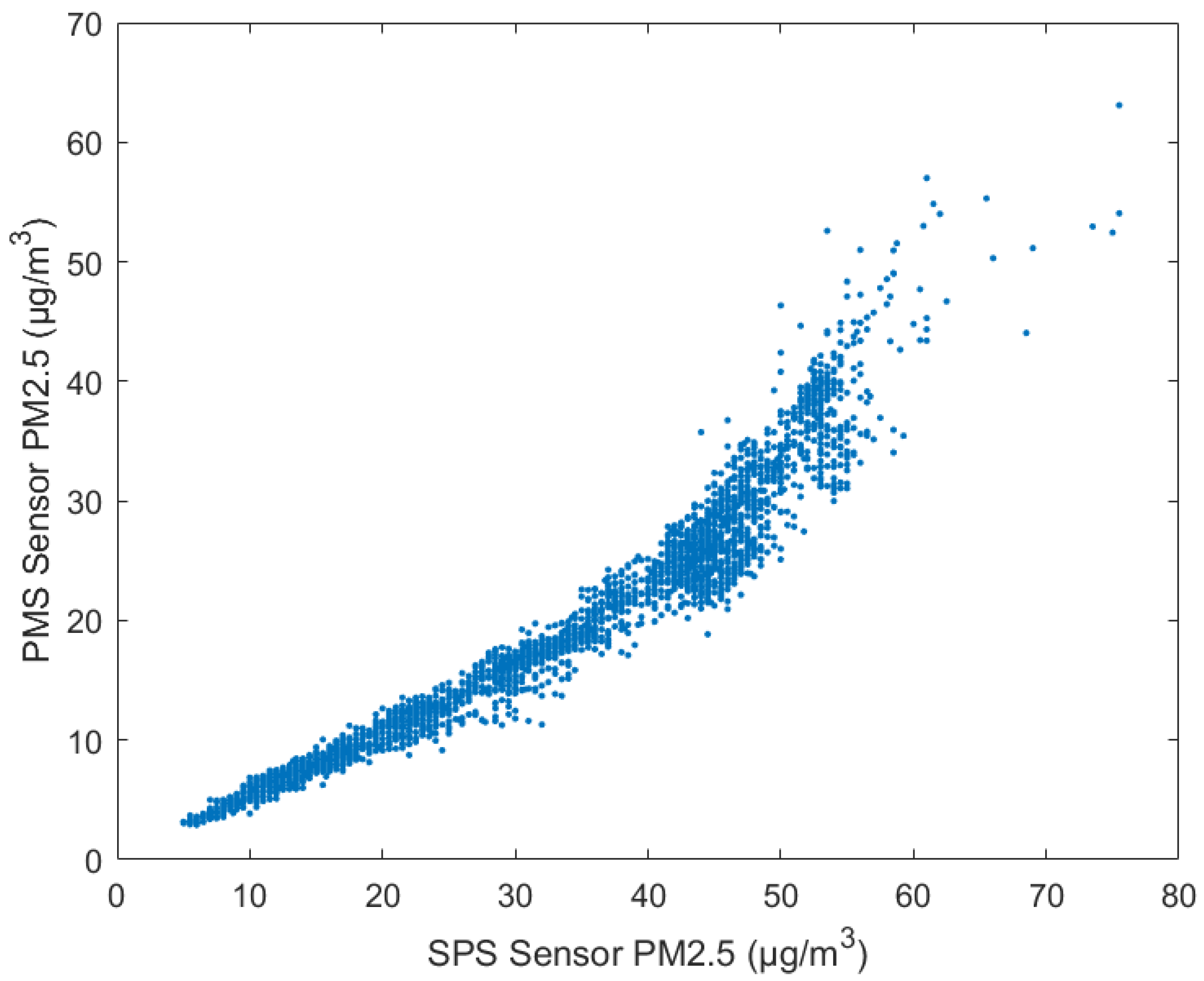
This sensor network consists of low-cost pollution monitoring sensors which are a compromise of low-cost and high-quality data [55]. The data captured by both types of sensors are directly compared in Figure 5. Comparing both the PMS and SPS sensor readings shows that the PMS sensor tends to provide higher concentration values compared to the SPS sensor; however, both sensor types show very close trends giving confidence to the accuracy of the measurements. The spread of the data is slightly broader at higher measured values, showing a higher uncertainty for the more extreme events. Other work has developed better calibration methods for these sensors against more accurate reference data so that for future pollution monitoring there would be a reduction in discrepancy [56].

3.2. The Gaussian Plume Model in ADMS and Settings

Initial analysis was made in this study using the ADMS software package [2,52], which is based on a Gaussian plume model. With this model based on empirical plume spread parameters taking account of the meteorological conditions such as wind conditions and temperature, the pollutant concentration at any point resulting from a defined source can be estimated. The ADMS version used in this study was 5.01.03 [52]. ADMS takes a few simple inputs which include source conditions, meteorology data, and geographical terrain information to predict the extent of pollution dispersion.
It should be noted that the ADMS package has some limitations for the current study. As the software was designed mainly for pollution analysis over large periods such as months or years, it is set up for 1-h intervals (time step). Therefore, it can estimate the pollutant (e.g., PM2.5) concentration for each 1-h interval in a steady manner, while for a point source short-distant dispersion problem 1-h emission time is much longer than many published case studies (e.g., [4]). The ADMS v5.01.03 cannot take account of the history of previous time steps, and therefore, cannot simulate point-source dispersion with a varying emission rate or in transient winds.
In this study, the fire was estimated as a point source. The diameter of the source was estimated to be 5 m with an elevation height of 1 m, in order to best match descriptions of the outbuilding from the news and fire reports [43,44]. For a heated point source, the plume rise model is used which elevates the source taking into account the buoyancy and momentum of the plume.
Two crucial parameters, i.e., the emission rate and the fire temperature of the source, were not able to be estimated solely by using ADMS. Instead, they were estimated from a systematic comparison between the CFD simulations, the ADMS simulations and the sensor data (see Section 5.3) considering the uncertainties involved in the approaches, as well as compared to a number of references [2,57,58,59]. A base source emission rate of 50 g/s and a base source temperature of 500 °C were estimated (see Section 5.3). The molecular mass was set to 62 g/mol and a specific heat of 1.55 J/g/K for nitrate [60].
The meteorological data were input into ADMS from the Met Office open-access data [48] covering the conditions at the time of the fire (Section 2.2), including the background ABL stratification condition. Short-term averaging was used in the calculations to obtain a smaller temporal resolution output of 1-h intervals compared to the default long-term model averaging over 24 h.
Geospatial data were provided using Ordinance Survey maps in Geo TIFF file format [61]. A roughness length was then set in ADMS to account for the type of terrain. As the city of Southampton is built up with a vast amount of buildings densely spaced of different heights up to 50 m, a roughness length z 0 of 1.5 m was used. ADMS has a graphic interface known as Mapper in which the Ordinance Survey map can be visualized, the location of sources placed, and the solution viewed. A grid is required to compute the calculations and a total of 62,500 equally spaced points was used. All other unspecified settings for the ADMS were left as default. ADMS gives a fast prediction of a steady solution of the scalar concentration field.

3.3. Large-Eddy Simulation in OpenFOAM and Its Settings

An open-source high-fidelity LES code embedded in the CFD package OpenFOAM v2.1.1 was used for simulations of the time-dependent puff release from the fire. OpenFOAM is a finite volume method (FVM) based CFD software package [36]. It has been released as an open-source package since 2004 and has become widely used in academia and industry. Although it is an open-source package, OpenFOAM has a number of features that require the end-user’s involvement to set up, such as the implementation of the inflow turbulence generation method (e.g., [4,34]). The LES method with the temporal and spatial discretization schemes in second-order accuracy was used in all simulations. The mixed time scale Sub-Grid Scale (SGS) model was used to avoid using the near-wall damping functions as used in the Smagorinsky SGS model.
Digital maps and Ordnance Survey information were used to construct a 15 km × 15 km CAD model of the city including buildings and terrain. The final CFD domain (Figure 6) is 3450 m (streamwise, x coordinate) × 2200 m (spanwise, y coordinate) × 1000 m (vertical, z coordinate) with a four-meter resolution within and above the urban canopy (Figure 7). The streamwise direction is the 310° wind direction (north-west).
The meshing approach in this study used the snappyHexMesh mesher built into OpenFOAM. This method allows flexible and robust mesh refinement. The size of the mesh is important to ensure a reasonable level of eddies is resolved, aiming to capture 80% of the turbulent kinetic energy. Three levels (4 m, 8 m and 16 m) of refinement were used, resulting in a total cell count of 25 million which was used throughout this study. Refining to 2 m at ground level did not significantly alter the results but increased the cell count to 100 million and significantly increased computational costs. Figure 7 shows the mesh at two levels of zoom in the domain. The dimensionless inflow mean velocity and turbulence statistics for synthetic turbulence generation were the same as in [4,62] in neutral conditions, which were obtained from wind tunnel experiments and linearly scaled [63] to match the freestream wind speed and turbulence intensity. Zero gradient outflow boundary conditions were used for the outlet. No-slip wall boundary conditions were used to enforce zero velocity at the ground and the building surfaces. Symmetric boundary conditions were used for the lateral and top boundaries.
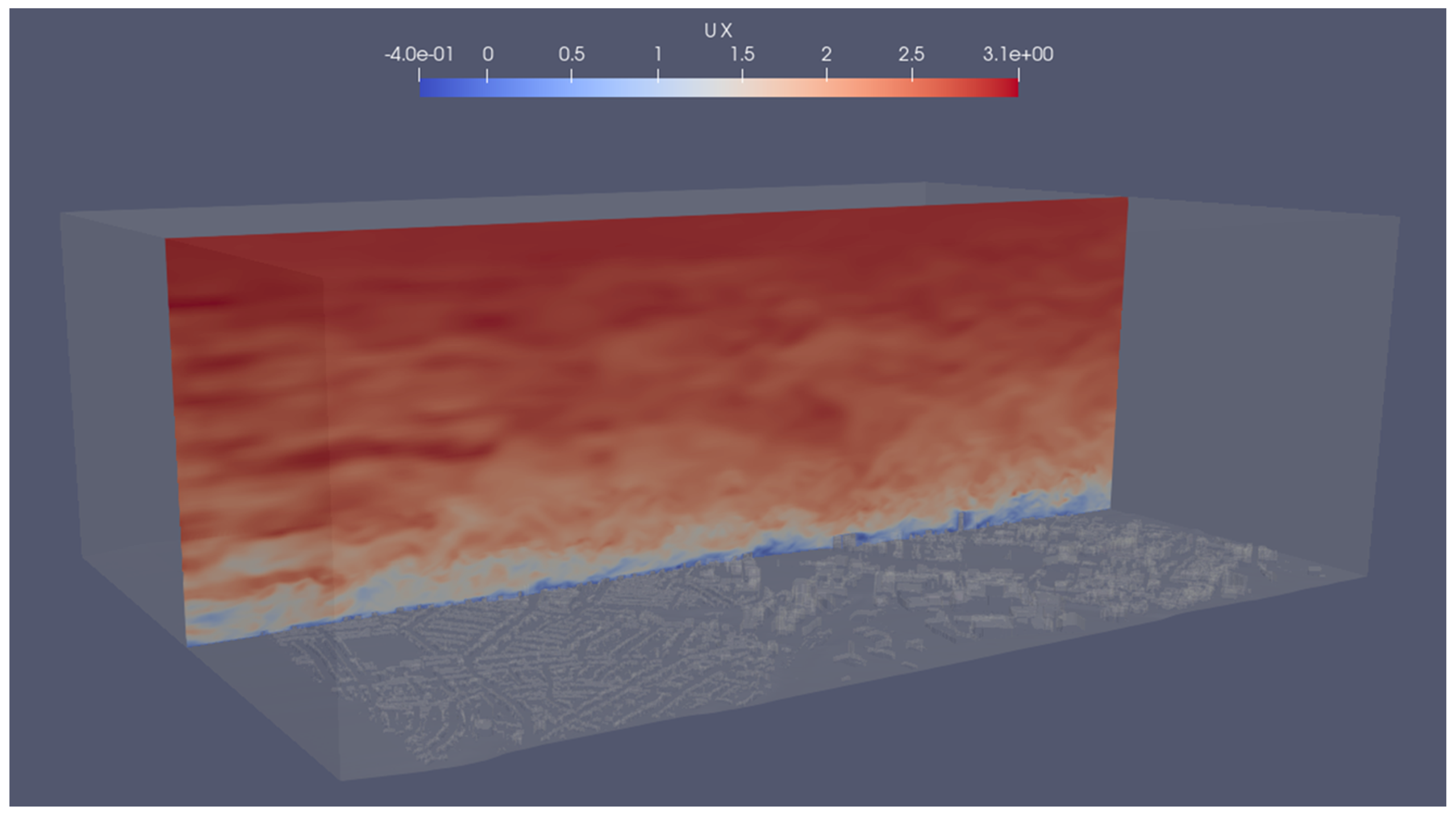
A very high temporal resolution with a small time step of 0.4 s was used, which satisfied the condition C F L < 1 . After a sufficient initialization duration for the flow to fully develop, the source started to release at t = 0 . It took less than 48 h of wall-clock time using 320 processors to finish one case. An example of the simulated instantaneous wind velocity field is presented in Figure 8. To assess the effect of the duration of the fire, without having to run multiple simulations, four different species with varying emission periods were set up in the simulation.

4. Measured PM2.5 Concentration from the Sensor Network

Section 3.1 has demonstrated the sensor accuracy by comparing the two data from the two different types of sensor. In this section, the measurements from the two types sensors during the fire incident are further analyzed.

4.1. Verification of the Sensor Measurement during the Fire Incident

The data acquired from the sensor network before, during and after the fire incident are analyzed. We focus specifically on the PM2.5 concentrations. This study estimates the air pollution resulting from the fire as the difference between typical daily pollution levels and the pollution level measured during the fire incident.
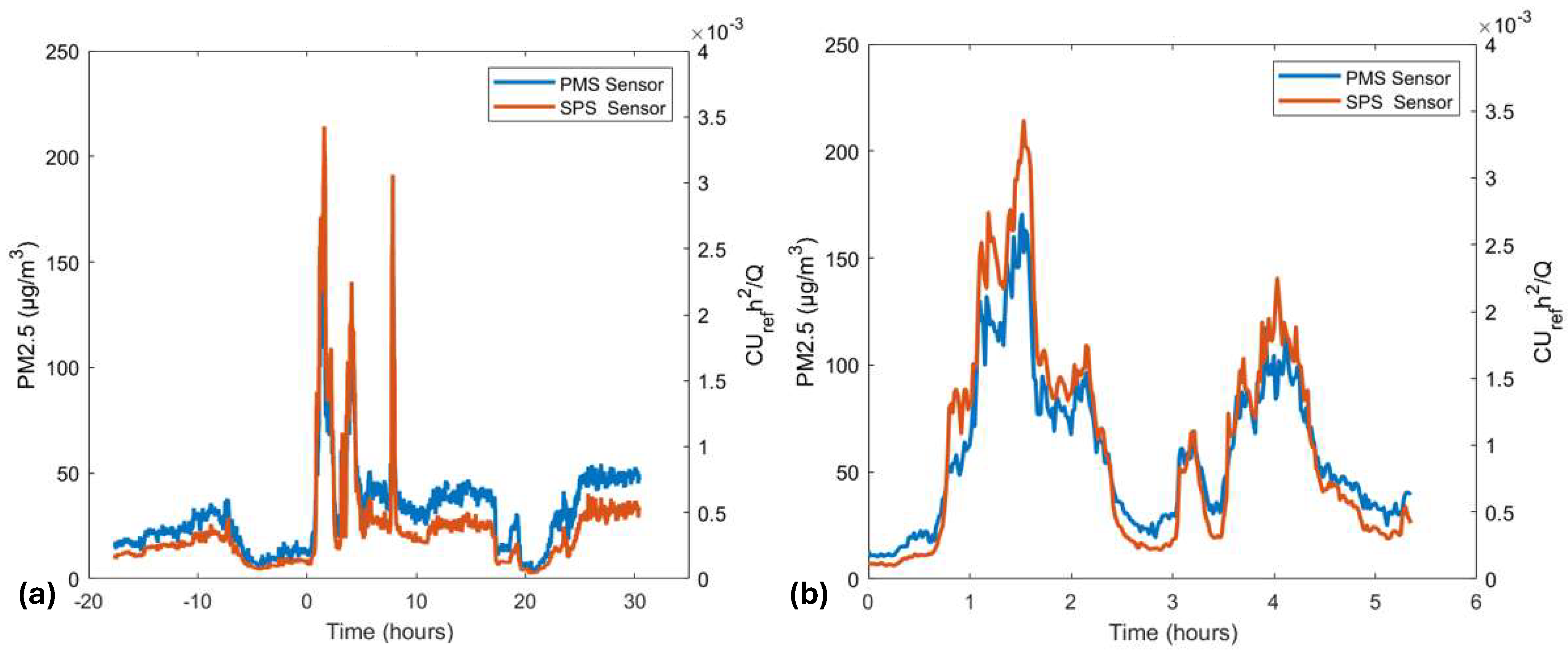
As there was a predominant steady north-westerly wind several hours before and five hours after the start of the fire (Figure 2 and Figure 3), only the sensor directly downwind of the fire detected a significant change in the PM2.5 concentration. The location of the downstream sensor is shown in Figure 1 just north of St Mary’s Football Stadium. The concentration measured by this sensor is shown in Figure 9a with clear spikes following the start of the fire with magnitudes greater than two to three times the background levels, demonstrating the effectiveness of the low-cost sensor. Figure 9b zooms in on the time of the fire and shows a good agreement between the SPS and PMS sensors, demonstrating the confidence of the measurements.

4.2. Estimation of the Fire Start Time from the Sensor Data

There is an initial time delay from the start time of the fire to the time that a spike was seen in the sensor data. This delay is the travel time of the pollutant cloud being advected from the fire site to the sensor by the mean advection velocity of the wind U a d v . The advection time, T 50 , is defined as the elapsed time (since release starting time) when the ensemble-averaged concentration reaches 50% of its local maximum at the sensor location and can be estimated as (e.g., [62])
T 50 = D U a d v ,
where D = 1500 m is the distance from the fire site to the sensor location. Xie et al. [62] suggests that typically U a d v = 0.15 U , where U is the freestream velocity, which was estimated to be 3 m/s in Section 2.2. This leads to the advection time T 50 = 0.9 h in the current case study. Considering the elapsed time T 50 against the sensor-measured concentration time series, the fire start time (at 17:30) is estimated, which is 28 min earlier than the news and the HIWFRS reports [43,44]. Figure 9b confirms that at T = 0.9 h, the concentration of PM2.5 reaches about 50% of the peak concentration. In summary, the estimation of the fire start time is reasonably accurate with an uncertainty of 10 min.

4.3. Discussion of the Fire Duration Based on the Sensor Data

Figure 9b shows that the PM2.5 concentration reaches a first peak at T = 1.5 h, then drops abruptly, and reaches a second spike at T = 2 h. Looking at wind direction data at the time of the fire (Figure 3), the wind direction was northwest at 0 T 1.5 h, forcing the pollutant plume to pass over the sensors. Likely due to the change in wind direction to a southwesterly wind after T = 1.5 h, the measured concentration drops abruptly. Afterward, the wind speed dropped to approximately 1 m/s at T = 2 h (Figure 2), resulting in a second low peak of PM2.5 concentration at the T = 2 h. In the first 2 h, the wind was overall in a steady state, and the pollutant release rate was likely more steady than in other periods [43,44,46]. This suggests that the numerical simulations and data analysis should focus on the first two hours.
During 2 T 3 h, the wind was mostly in the south-west or west directions, shifting pollutant plume away from the sensors (assuming the fire was still actively emitting pollutants), resulting in a lower PM2.5 concentration at T 3 h. During 3 T 4 h, the wind direction again changed from north–northwest to northwest, and to north, resulting in a narrow peak at T = 3.3 h and a broad peak at T = 4 h. During 4 T 6 h, the wind direction was initially from the north, and later changed to the northeast, resulting in a sudden drop in sensor measurements. In summary, during 2 T 6 h, the wind direction was very complicated, it would be extremely challenging to carry out numerical simulations and comparison with the sensor data if the simulations were not driven by ’real-life’ winds varying in direction and magnitude. Therefore, the period 2 T 6 h is not the focus of the study.

5. Numerical Simulations and Estimation of the Emission Rate

This section is to use numerical data to confirm the fire start time of 17:30 estimated in Section 4.2 from the sensor data and to estimate the emission rate. The fire duration is also discussed again.

5.1. Estimated Concentration from ADMS

The Gaussian plume model in the ADMS package was used to efficiently produce initial results taking into account the thermal buoyancy effect by inputting an initial guess of 500 °C for the fire temperature. The detailed settings are presented in Section 3.2. The wind speed and direction, respectively, shown in Figure 2 and Figure 3 were assumed to be constant over 60 min intervals. Again, the study was focused on the period 0 T 2 h, when the wind direction was more steady and the pollutant emission rate was more likely constant.
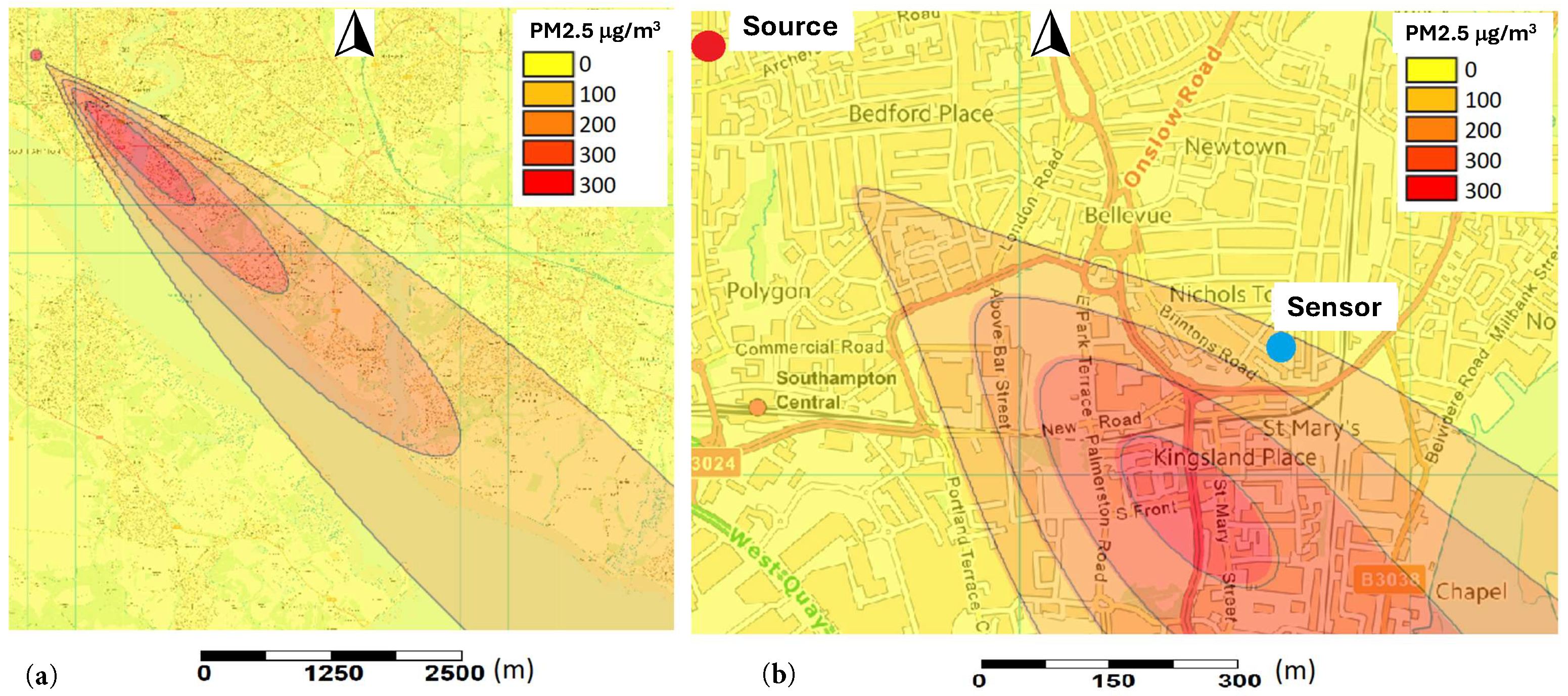
The contours of ground level PM2.5 concentration at T = 1.5 h are visualized in Figure 10, showing the plume is aligned with the wind direction. The maximum value of PM2.5 concentration occurs downstream of the source, which is due to the thermal buoyancy effect being taken into account in ADMS. Figure 10 shows that the sensor was located just inside of the PM2.5 plume. This also suggests that when the wind became more northerly at T = 4 h, the plume shifted off the sensors and was no longer measured. The fire temperature was assessed in ADMS and is discussed in Section 5.3.

5.2. Estimation of the Fire Start Time from OpenFOAM

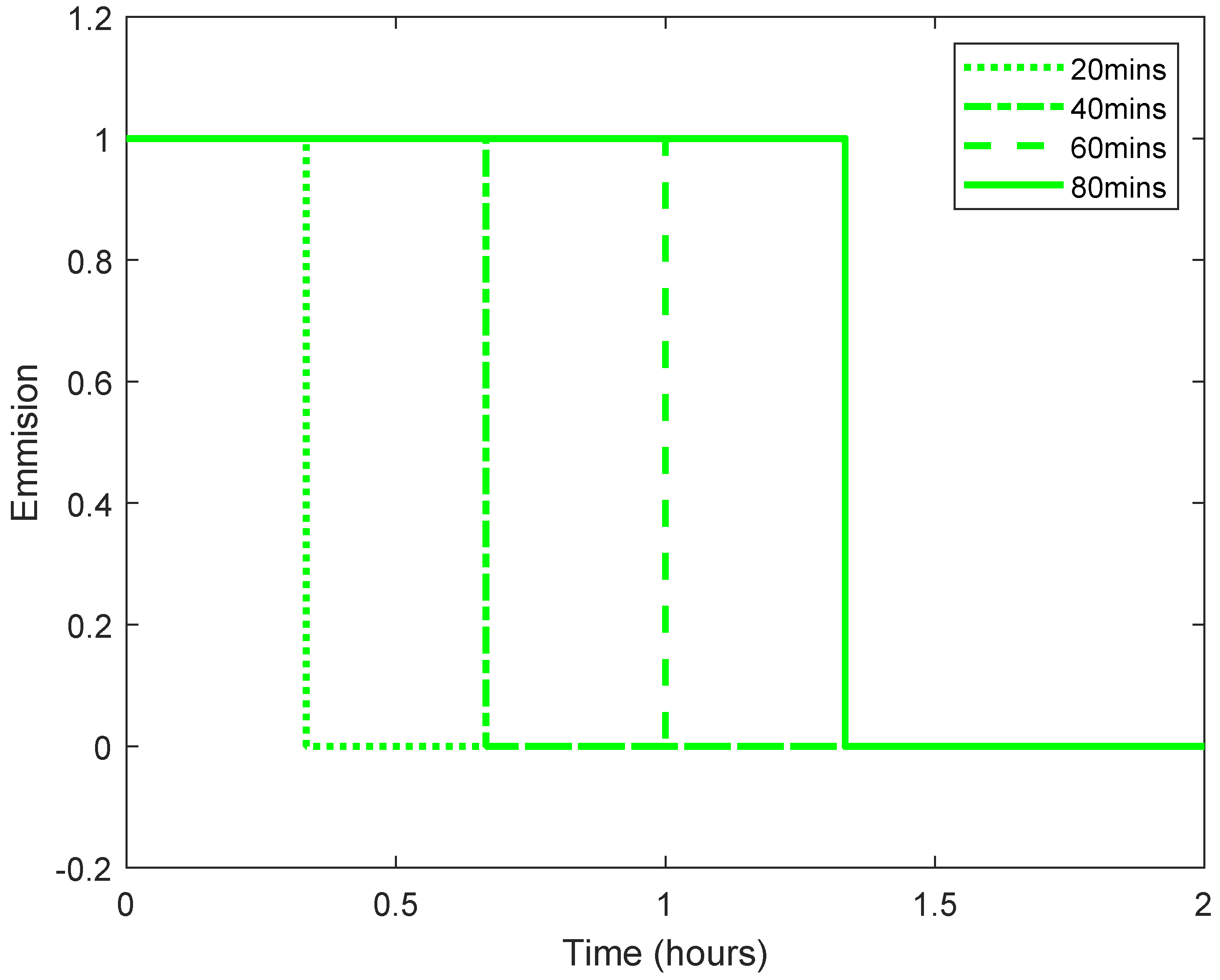
Following Section 4.3, this study focused on the period of a steady wind in the first 2 h; several LES tests were carried out to assess the sensitivity due to the uncertainty of the start time and duration of the fire. Four different scalar species were released at the same rate Q = 50 g/s, at the same time and at the same location where the fire broke out, with release periods of 20 min, 40 min, 60 min and 80 min, respectively. The four sources each had the same spatial size (5 m × 5 m × 5 m). The time series of the emission rate normalized by Q = 50 g/s for each source is shown in Figure 11. To simplify the LES settings, the wind direction and speed were kept constant, which were based on the fact that the wind was nearly steady in the first 2 h from the fire start (Figure 2 and Figure 3). The evident variations in wind speed and the small variations in wind direction during the first 2 h of the fire are taken into account when comparing the LES data to the sensor data in Section 5.3.
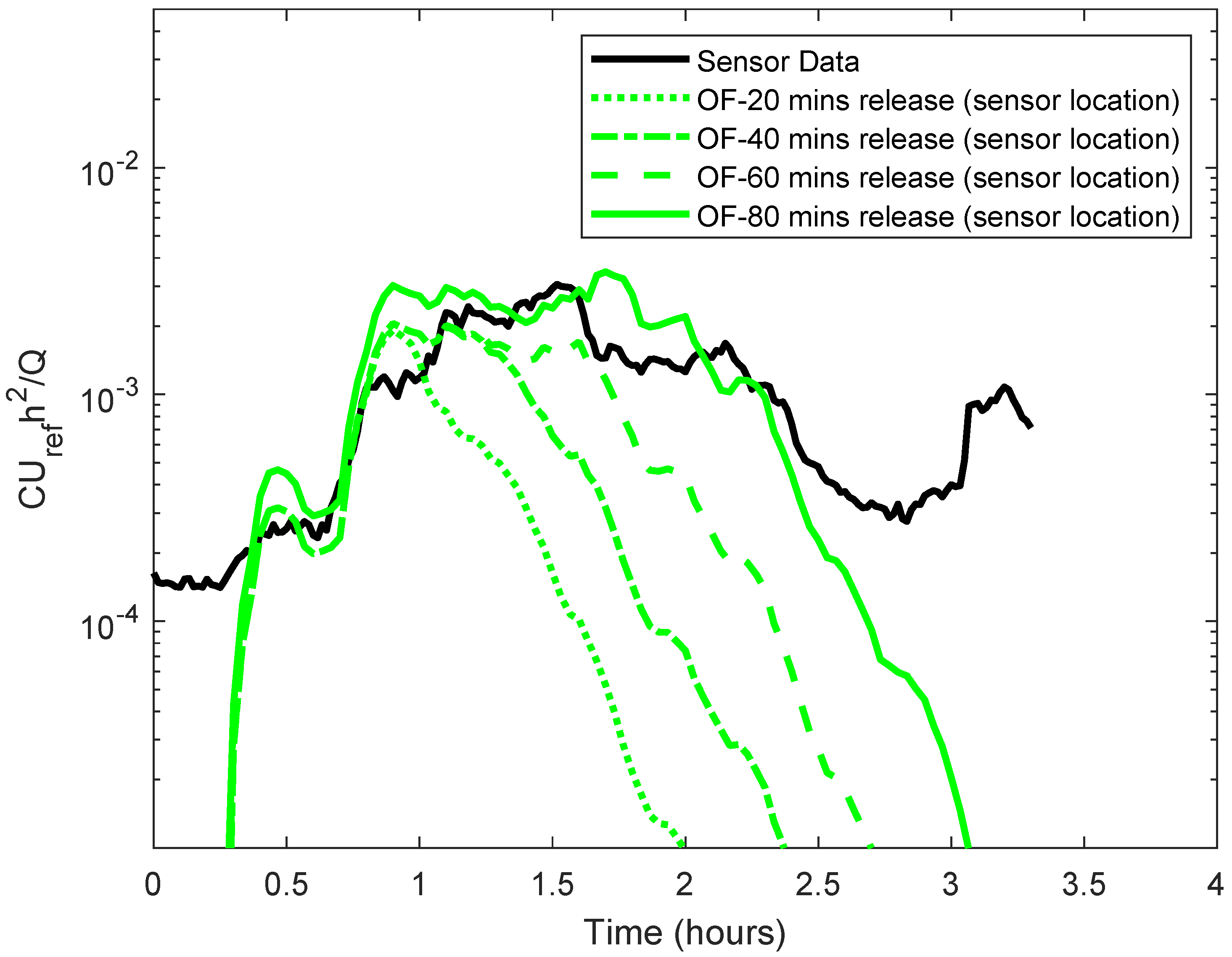
Figure 12 presents the simulated concentration at the sensor location from the four releases, non-dimensionalized based on the estimated emission rate Q = 50 g/s, the reference velocity U r e f , and the averaged building height h = 16.5 m/s. As a baseline, the dimensionless sensor data based on the same characteristic quantities are also shown in Figure 12. Here, the sensitivity tests address two key questions: (1) what time the fire started, and (2) how long the fire lasted. Other key questions, e.g., the emission rate assumed to be 50 g/s in Figure 12, are discussed extensively in Section 5.3.
Comparing the four sets of CFD data to the sensor data shown in Figure 12, we can conclude that the 80-min release produces results from CFD with the closest match to the sensor data, both having an approximately 80-min period with a concentration greater than 50% of its local maximum. Note, that Figure 3 shows a very steady wind direction in the first 2 h time, at an average freestream wind speed of 2 m/s (Figure 2), which is the windiest period during the entire fire event. Therefore, we conclude that the LES gives the most reliable prediction in the first 2 h, confirming that the fire started at 17:30 and lasted steadily for at least 80 min producing nearly constant emission of pollutants.
At T = 2 h, the wind changed from north-west to south-west (i.e., 250°), shifting the plume out of the reach of the sensors (see Figure 1), leading to a sudden concentration drop shown in Figure 5. It is not clear whether the sudden drop was solely due to the change in the wind direction, or also due to the possible reduction in the release rate, since the firefighter crew started at 18:00 to control the fire [43,44,46]. This results in great uncertainty in the estimation of emission rate at the T = 2 h time and afterwards. At T = 3 h time, the wind direction changed to north-west (330°), shifting the plume back in the sensors’ reach range and leading to a small concentration peak. At T = 3.5 h time, the wind direction changed to 310° and stayed for about 1 h, leading to a second greatest concentration peak (Figure 9b). Given the wind speed at T = 4 h time is only one-third of that in the first 2 h, and the measured PM2.5 concentration at T = 4 h is about half of the peak concentration in the first 2 h, one can deduce from the dimensional analysis that the emission rate must be significantly reduced at earlier than T = 4 h time, considering the advection time. At the T = 5 h time, the wind changed to a northerly direction, and the sensors were entirely out of the plume even if the remainder of the fire was still emitting pollutants. Due to the greater uncertainty after T = 2 h time, hereafter, only the 80-min release in the CFD is considered. Again, 80 min release along with the steady wind is more than five times longer than the 15 min release (e.g., [4,62]) for a puff release study, and should be enough for an estimation of the emission rate in Section 5.3.
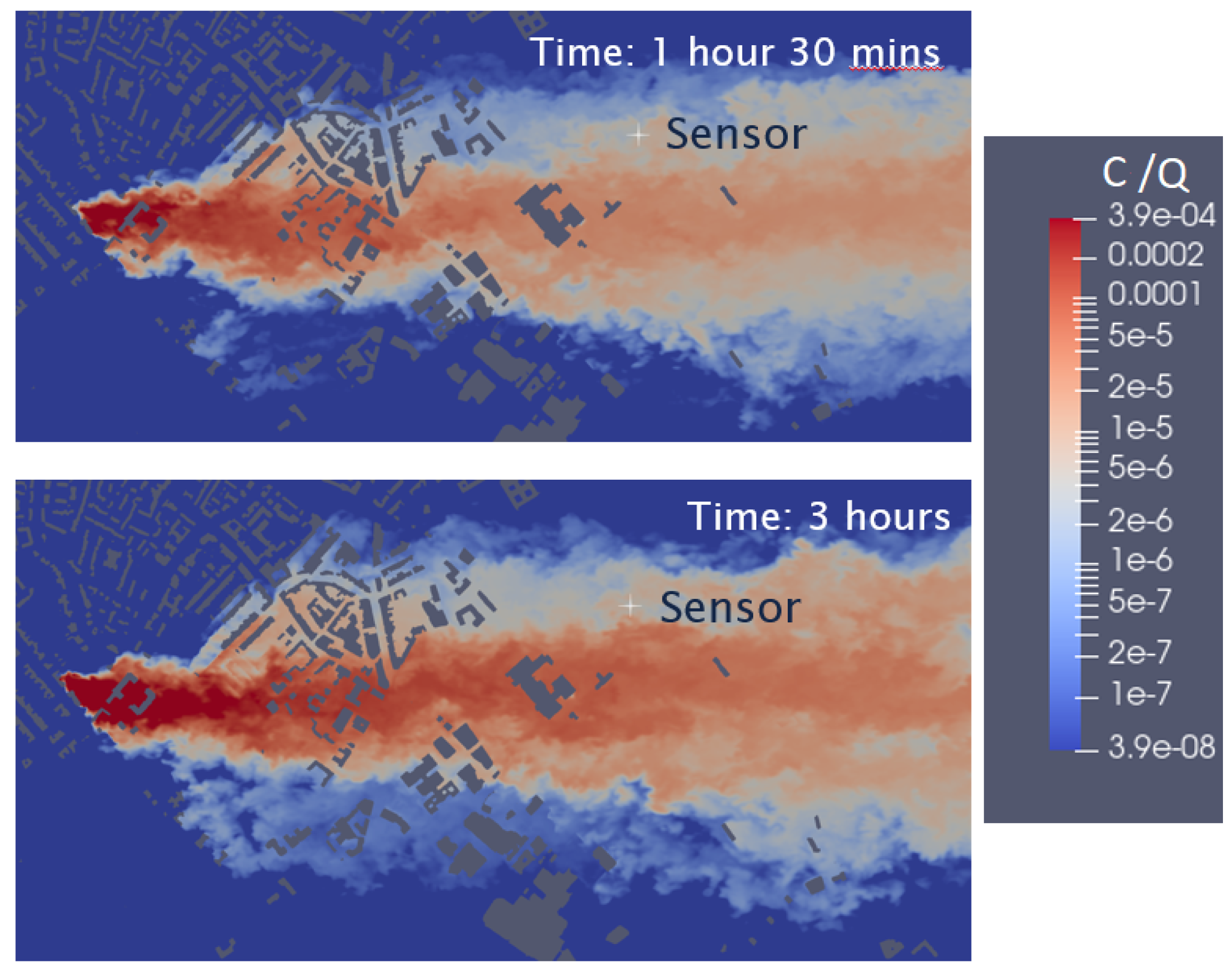
Visualization of the PM2.5 concentration from the LES in OpenFOAM is a key advantage compared to using sensors and the ADMS software package. Figure 13 shows ground-level concentration contours, which are similar to the PM2.5 concentration contours shown in Figure 10 from the ADMS simulations. Both the LES and ADMS data confirm that the sensor was located inside the plume. Nevertheless, there are evident differences between Figure 10 and Figure 13. For example, the former shows a cross-wind symmetry over the entire streamwise range, whereas the latter shows an asymmetry in the near field, which is due to the street canyon effect captured in the LES. The LES in OpenFOAM produced four-dimensional data (i.e., three-dimensional in space and one-dimensional in time). Figure 12 and Figure 13 clearly show extremely rich details.

5.3. Estimation of the Emission Rate from Available Data

In this section, the two different modeling methods used in this study were compared to the sensor data. As discussed earlier, ADMS cannot produce transient solutions. Here, the ADMS outputs are the time-averaged steady-state results for a one-hour period. Under the quasi-steady meteorological conditions in the first 2 h, the concentration sampled at the sensor location from the OpenFOAM 80-min release shows a near-constant value during a period of approximately 1 h (Figure 12). The average of the 1 h concentration is considered as the maximum concentration. The period with a concentration greater than 50% of the maximum concentration is considered as the local plume duration, which is slightly over 1 h. The time-averaged concentration during this period is denoted as the mean concentration.
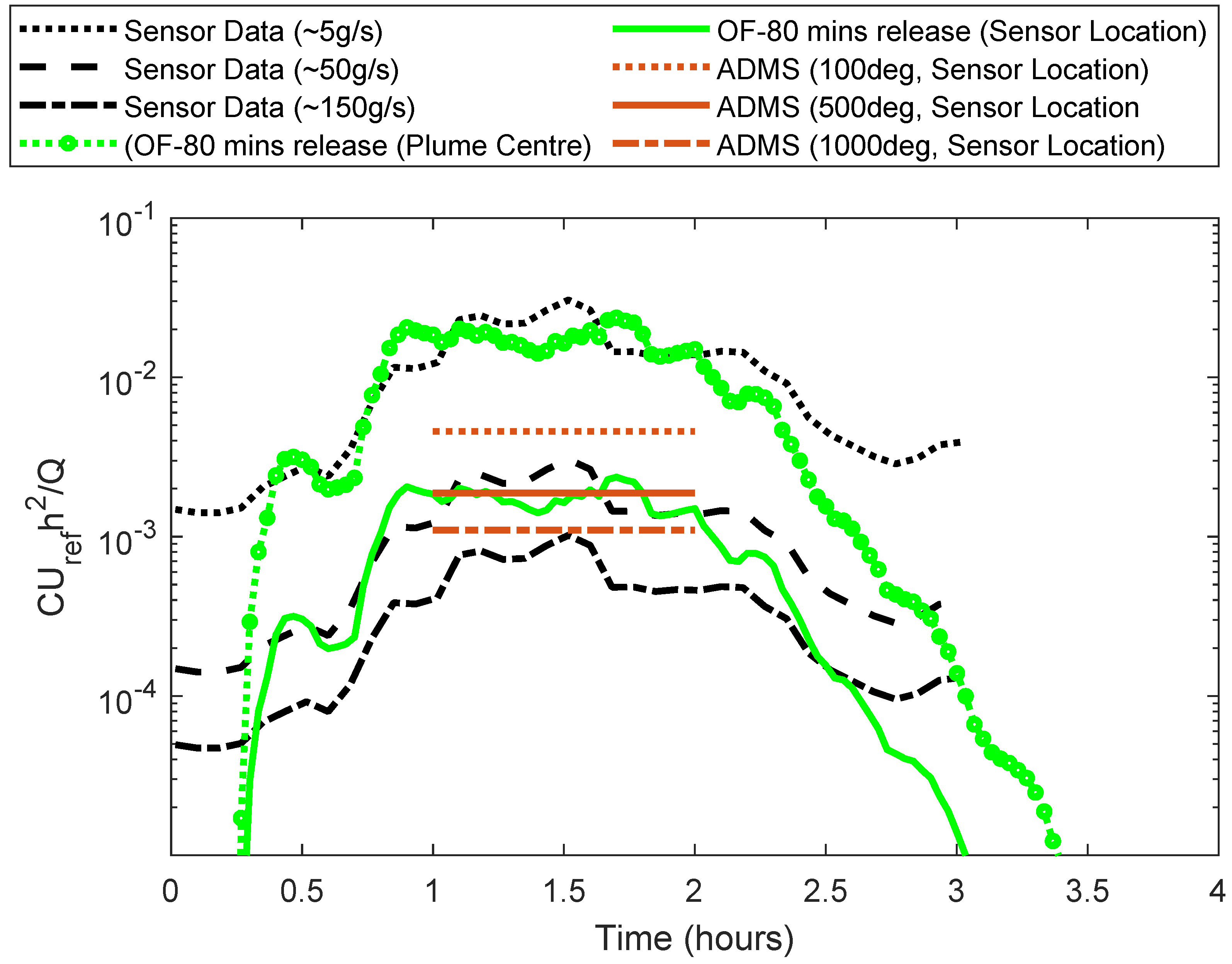
In Section 4.2 and Section 5.2, the fire start time and duration have been addressed. In addition to these, the emission rate as well as the high and localized fire temperature uncertainties must be estimated when comparing the ADMS and CFD data to the sensor data. To check the uncertainties due to the estimation of the fire temperature, three guesses 100 °C, 500 °C and 1000 °C were made for the fire temperature considering published reports [47], and were tested in ADMS with the same emission rate. To check the uncertainties due to the sample location relative to the plume center, two sample locations, i.e., one at the sensor site and one at the plume center, were tested for the ADMS data and for the OpenFOAM data. To study the effects due to fire temperature and emission rate, Figure 14 shows a comparison between the sensor measurements, ADMS, and CFD concentrations in non-dimensional form as c ^ = C U r e f h 2 / Q . Three guesses of 5 g/s, 50 g/s and 150 g/s were made for the emission rate Q, from which we endeavored to choose a more possible one in the following paragraph.
The large variation of the fire temperature evidently changed the dimensionless concentration c ^ up to four times. Figure 14 shows that increasing the fire temperature from 500 °C to 1000 °C in the ADMS settings, c ^ converges asymptotically to some constant. According to Cote [47], “the average peak temperature of a house fire is around 593 °C”. Therefore, an average fire temperature of 500 °C over the first 2 h time in the incident is a more reasonable guess. The sensor measurements ‘Sensor Data (50 g/s)’ were the best match with the ADMS data ‘ADMS (500Deg, Sensor Location)’, suggesting an emission rate Q = 50 g/s and a fire temperature 500 °C in the first 80 min of the fire. The CFD data ‘OF-80 min release (Sensor Location)’ fell into this range, confirming the suggested emission rate and the fire temperature.
The dimensionless concentration c ^ sampled at the center of the plume (i.e., the case ‘OF 80-min release, (plume center)’) with the same distance to the fire site is about one order of magnitude greater than that at the sensor location. Both the ADMS data (Figure 10) and the CFD data (Figure 13) show that the sensors are located at the edge of the plume in the steady 310° wind so it is unlikely that the plume center passed directly over the sensors during the fire incident.

5.4. Uncertainties and Confidence of the Estimation

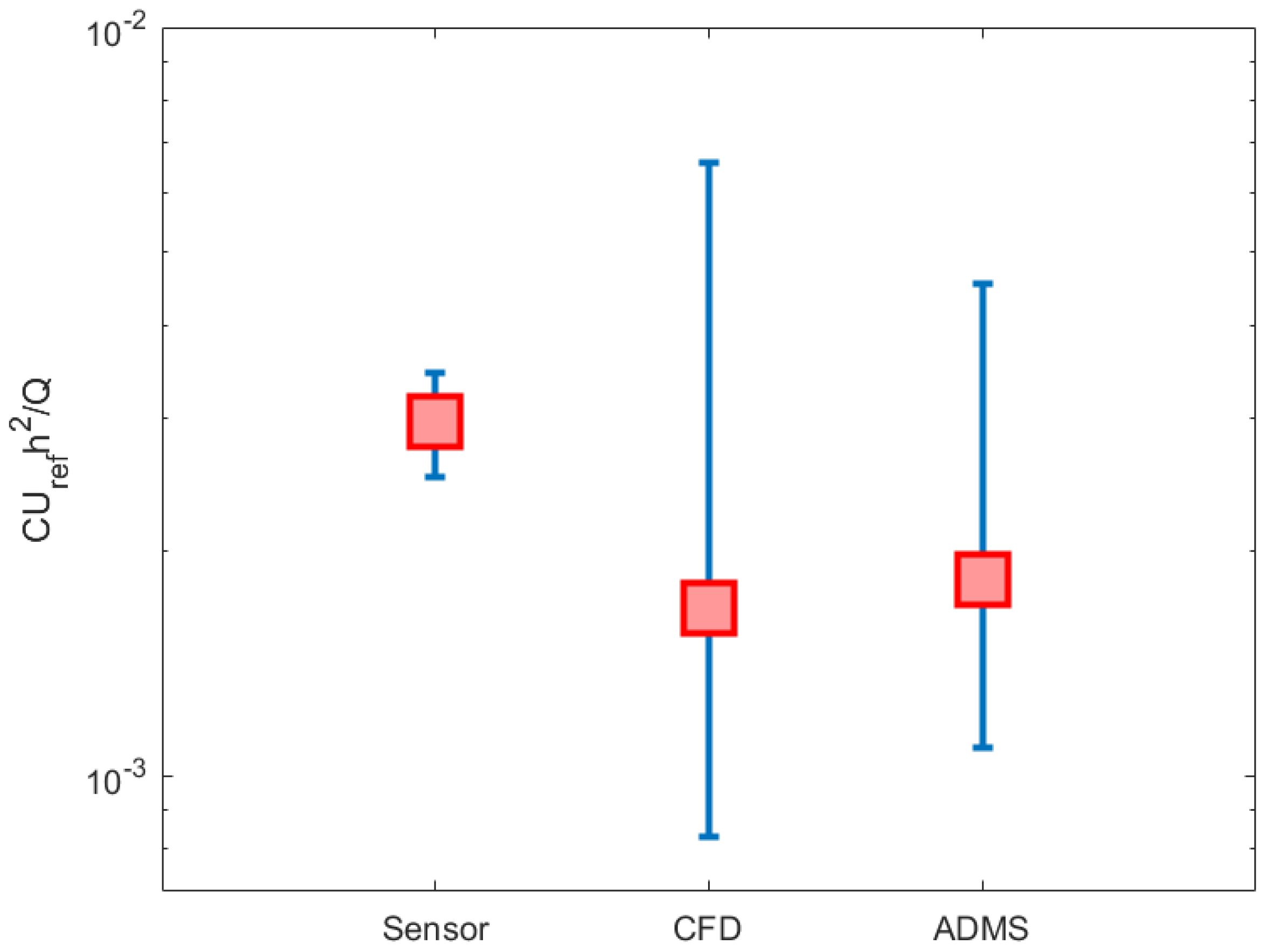
Figure 15 shows the dimensionless mean concentrations during the hours 1 T 2 obtained from all three methods together along with their uncertainties. The major sensor uncertainty is due to the background PM2.5 concentration, which is approximately 15% of the peak sensor data (Figure 9). The upper and lower error bars for the sensor data shown in Figure 15 are set, respectively, to +15% and −15% based on the sensor data.
The first CFD uncertainty is due to the assumption of the neutral stratification, ignoring the stable stratification in the background atmospheric boundary layer (ABL). The background ABL during the fire incident was diagnosed as being stable with a ratio z B L / L M O = 6 in Section 2.2, suggesting that the background ABL stability tended to suppress the plume to spread in the vertical direction and hence to increase the concentration at the sensor site. Sessa et al. [34] shows that a medium stable stratification in the background urban ABL can increase the concentration by three times compared to when the stability of the atmosphere is neutral. Considering this, the upper error bar for the CFD data in Figure 15 is set at three times the LES-predicted concentration.
The second CFD uncertainty is due to not considering the localized unstable stratification at the fire site. The local fire temperature increases the influence of buoyancy and effectively raises the source elevation. Fackrell and Robins [1] carried out wind tunnel experiments to investigate the difference of dispersion between a ground-level point source and an elevated point source at a height of about 0.2 z B L . They reported that the concentration measured at ground-level stations 3 z B L downstream or further of the elevated source was approximately half of that for the ground-level source. On the same stations 3 z B L downstream of the source, the plume size in the vertical direction for the elevated source was twice that for the ground-level source, while the plume width in the cross-wind direction was the same. At 17:30 2 December when the fire started, it was 1.5 h after the sunset time 16:00 in the UK. Kotthaus and Grimmond [64] show that the ABL thickness z B L over London was approximately 500 m at 17:30 in the winter time in similar meteorological conditions as the current case study. This suggests that the distance from the sensor station to the fire site was 3 z B L , more than the 1.5 z B L distance criteria noted in Fackrell and Robins [1].
The third CFD uncertainty is due to the assumption of steady wind direction settings, while real life is never strictly steady [4] even though the study was focused on the first 2-h period of the fire when the wind was in a nearly steady north-west direction. Xie [4] carried out a study on a ground-level point source dispersion in similar wind conditions, showing that a non-stationary wind can reduce the concentration to half compared to a stationary wind. It should be noted that both the effective elevated source and the variation of wind direction caused the meandering of the pollutant plume and the resulting reduced PM2.5 concentration on the ground level. As the sensor site was 3 z B L downstream from the source where the plume size in the vertical direction was close to the ABL thickness z B L (see Fackrell and Robins [1]), the lower error bar for the CFD data in Figure 15 is set being half of the LES-predicted concentration while Considering both the second and third factors.
The ADMS uncertainty is due to the estimate of the fire temperature. Fire temperatures of 100 °C and 1000 °C were also simulated using the ADMS package, respectively, corresponding to the upper and lower error bars for the ADMS data. Both Figure 14 and Figure 15 show that the dimensionless concentration tends to asymptotically converge for fire temperature greater than 500 °C, suggesting a likelihood of small error due to the fire temperature estimate.
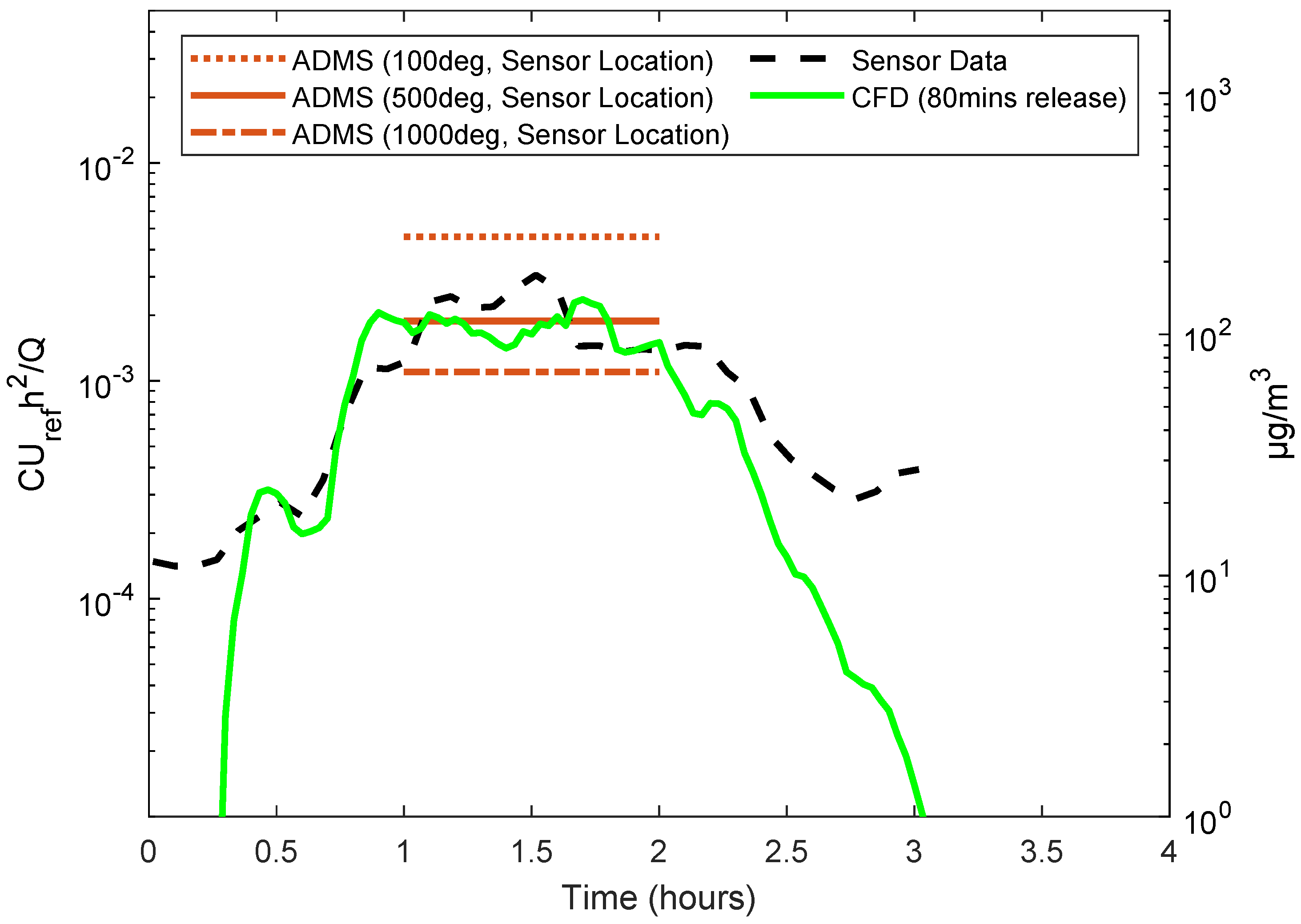
The error due to the estimate of the emission rate is usually not small and is not presented in the dimensionless concentration plots in Figure 15. Figure 16 brings together the concentration time series obtained from sensor measurements, CFD and ADMS predictions. The CFD and ADMS predictions are based on an estimated emission rate of 50 g/s, which is much greater than the value of 1 g/s used by Carruthers et al. [2] and in the ADMS 6 Buildings Validation Warehouse Fires Wind Tunnel Experiments [28]. Compared with the case study of [2], which reported a measured peak concentration of around 1 μg/s at 487.5 m downwind to the fire site, the measured peak concentration from the Southampton fire is about 100 μg/s measured about 1500 m downwind from the fire site, suggesting that the estimated emission rate in the current study is within a reasonable range. The burnt material was mainly highly flammable cine nitrate film, which produced a massive amount of particulate matter. A comment from a resident living 2500 m downwind of the fire provided consistent evidence to support this estimate (see [43] and Section 2.1).

6. Discussion and Concluding Remarks

While monitoring air pollution in the City of Southampton, a fire broke out which caused a significant release of smoke in the region. Using measurements from the sensor network, the key objective of this work is to present a unique case study for predicting pollutant PM2.5 concentration from urban fires using both low- and high-fidelity numerical models, aiming to explore the capability of the low-fidelity numerical model—ADMS for fast response, and the accuracy of the high-fidelity numerical model—large eddy simulation embedded in OpenFOAM for such applications.

6.1. Advantages and Limitations of Both Numerical Approaches, and Their Potential Roles in Fast Response Applications

Designing an integrated tool for fast response is always a compromise of economic cost and required accuracy. This study used the most efficient approach—Gaussian plume model embedded in ADMS (a full-parameterization method) and the most accurate but computationally expensive approach—large eddy simulation embedded in OpenFOAM (a full-CFD method)—to estimate pollutant dispersion from an urban fire. Using the two extreme approaches can explore the capabilities of the fast response tools including the intermediate-level tools, such as the FAST3D-CT model [29] and the street-network models [11,30]). The advantages and limitations of these tools scatter in a very wide range and it is not possible to present a complete list. More studies on high-resolution modeling of urban air quality can be found in a review paper (e.g., [37]). Table 1 presents an unexhaustive list of the advantages, limitations and potential applications of the Gaussian plume model (GPM) and the large-eddy simulation (LES) for prediction of pollutant dispersion from an urban fire.
Fourteen aspects are compared in Table 1 between the LES and GPM models. These can be grouped into four categories. The first category is resolution and accuracy, i.e., spatial and temporal resolution, and output data, in which LES has a higher resolution and accuracy. The second is efficiency and complexity in the use of the software packages, i.e., complexity in setup, user experience level, computational cost (CPU hours), and efficiency (wall-clock mins), in which GPM is more efficient and simpler to use. The third is the inclusion of physical parameters, i.e., wind speed and direction, wind vertical profiles, etc., ABL stability, and fire buoyancy effect, in which LES has more potential than GPM. The fourth is the potential applications for the considered areas. Currently, GPM can be used for some fast response problems as demonstrated in this case study, while LES data can be used to improve the GPM parameterization schemes. In the near future (e.g., in ten years time), LES with supercomputers can hopefully be used for fast response problems [31], while developing an integrated tool including geometry and mesh generation, running LES faster than real-time, and visualizing the LES data, is the top priority.

6.2. Concluding Remarks

By comparing the sensor measurements, the ADMS data, and the LES data, an iterative process is presented, which demonstrates that the Gaussian plume model embedded in ADMS can produce a fast estimate of the smoke plume extent and magnitude at a distance of more than 1500 m downwind of the fire. In addition, six points must be emphasized here: (1) Real-life sensor measurements are always useful, such as for calibrating the numerical models and checking the fire start time and duration. (2) Using the real-life meteorological data is of crucial importance for setting up the numerical models, as well as for understanding the sensor data, etc. (3) Depending on the burnt materials, the emission rate of pollutants in one incident can be one order of magnitude in difference compared to another. Identifying the burning materials is of crucial importance for the estimate of the emission rate. (4) The Gaussian plume model in ADMS can give a reasonable prediction at downstream 1000 m if the emission rate can be estimated based on a database and the meteorological conditions are known. (5) Large-eddy simulations can be useful to improve the parameterization schemes in the ADMS models, such as for the near-source dispersion from an urban fire. (6) For final decision-making, the relevant uncertainties, including the meteorological conditions, the emission rate, the fire temperature, the fire start time and its duration, must be taken into account.
This research provides a unique case study for testing fast response models for applications of pollutant dispersion from an urban fire. It also demonstrates the capability of using the Gaussian plume model for fast response, and the future potential application of using the large-eddy simulation model for near-field dispersion in fast response applications.

Author Contributions

Conceptualization, Z.-T.X. and C.V.; software, M.C. and D.C.; formal analysis, D.C.; sensor measurements and data curation, F.M.J.B. and S.J.C.; writing—original draft preparation, D.C.; writing—review and editing, Z.-T.X. and C.V.; supervision, S.J.C., Z.-T.X. and C.V.; funding acquisition, Z.-T.X. and C.V. All authors have read and agreed to the published version of the manuscript.

Funding

This research was funded by UKRI grant number MR/S015566/1 and NERC grant number NE/W002841/1. The APC was funded by the University of Southampton.

Institutional Review Board Statement

Not applicable.

Informed Consent Statement

Not applicable.

Data Availability Statement

Data will be made available at the University of Southampton data repository.

Acknowledgments

We would like to thank Florentin Bulot, who for his PhD built the low-cost sensor network and provided us with the data for the time of the fire in Southampton supervised by Steven Ossont and Simon Cox.

Conflicts of Interest

The authors declare no conflicts of interest. The funders had no role in the design of the study; in the collection, analyses, or interpretation of data; in the writing of the manuscript; or in the decision to publish the results.

References

  1. Fackrell, J.; Robins, A. Concentration fluctuations and fluxes in plumes from point sources in a turbulent boundary layer. J. Fluid Mech. 1982, 117, 1–26. [Google Scholar] [CrossRef]
  2. Carruthers, D.; Mckeown, A.; Hall, D.; Porter, S. Validation of ADMS against wind tunnel data of dispersion from chemical warehouse fires. Atmos. Environ. 1999, 33, 1937–1953. [Google Scholar] [CrossRef]
  3. Ambade, B. Characterization of PM 10 over urban and rural sites of Rajnandgaon, central India. Nat. Hazards 2016, 80, 589–604. [Google Scholar] [CrossRef]
  4. Xie, Z.T. modeling Street-Scale Flow and Dispersion in Realistic Winds—Towards Coupling with Mesoscale Meteorological Models. Bound.-Layer Meteorol. 2011, 141, 53–75. [Google Scholar] [CrossRef]
  5. Luo, X.; Bing, H.; Luo, Z.; Wang, Y.; Jin, L. Impacts of atmospheric particulate matter pollution on environmental biogeochemistry of trace metals in soil-plant system: A review. Environ. Pollut. 2019, 255, 113138. [Google Scholar] [CrossRef]
  6. Yim, S.; Li, Y.; Huang, T.; Lim, J.; Lee, H.; Chotirmall, S.; Dong, G.; Abisheganaden, J.; Wedzicha, J.; Schuster, S.; et al. Global health impacts of ambient fine particulate pollution associated with climate variability. Environ. Int. 2024, 186, 108587. [Google Scholar] [CrossRef] [PubMed]
  7. Hussain, A.J.; Sankar, T.K.; Vithanage, M.; Ambade, B.; Gautam, S. Black carbon emissions from traffic contribute sustainability to air pollution in urban cities of India. Water Air Soil Pollut. 2023, 234, 217. [Google Scholar] [CrossRef]
  8. Mole, N.; Anderson, C.; Nadarajah, S.; Wright, C. A generalized pareto distribution model for high concentrations in short-range atmospheric dispersion. Environmetrics 1995, 6, 595–606. [Google Scholar] [CrossRef]
  9. Xie, Z.T.; Hayden, P.; Robins, A.G.; Voke, P.R. modeling extreme concentrations from a source in a turbulent flow over a rough wall. Atmos. Environ. 2007, 41, 3395–3406. [Google Scholar] [CrossRef]
  10. Nelson, M.; Addepalli, B.; Hornsby, F.; Gowardhan, A.; Pardyjak, E.; Brown, M. 5.2 Improvements to a Fast-Response Urban Wind Model. In Proceedings of the American Meteorological Society 88th Annual Meeting, New Orleans, LA, USA, 22 January 2008; pp. 20–24. [Google Scholar]
  11. Hertwig, D.; Soulhac, L.; Fuka, V.; Auerswald, T.; Carpentieri, M.; Hayden, P.; Robins, A.; Xie, Z.T.; Coceal, O. Evaluation of fast atmospheric dispersion models in a regular street network. Environ. Fluid Mech. 2018, 18, 1007–1044. [Google Scholar] [CrossRef]
  12. Santos, J.M.; Reis, N.; Castro, I.; Goulart, E.V.; Xie, Z.T. Using large-eddy simulation and wind-tunnel data to investigate peak-to-mean concentration ratios in an urban environment. Bound.-Layer Meteorol. 2019, 172, 333–350. [Google Scholar] [CrossRef]
  13. Hankey, S.; Marshall, J.D. Urban Form, Air Pollution, and Health. Curr. Environ. Health Rep. 2017, 4, 491–503. [Google Scholar] [CrossRef]
  14. Künzli, N.; Tager, I.B. Air pollution: From lung to heart. Swiss Med. Wkly. 2005, 135, 697–702. [Google Scholar] [PubMed]
  15. Oudin, A.; Forsberg, B.; Jakobsson, K. Air pollution and stroke. Epidemiology 2012, 23, 505–506. [Google Scholar] [CrossRef] [PubMed]
  16. Maximillian, J.; Brusseau, M.; Glenn, E.; Matthias, A. Pollution and Environmental Perturbations in the Global System, 3rd ed.; Elsevier Inc.: Amsterdam, The Netherlands, 2019; pp. 457–476. [Google Scholar]
  17. Cohen, A.J.; Brauer, M.; Burnett, R.; Anderson, H.R.; Frostad, J.; Estep, K.; Balakrishnan, K.; Brunekreef, B.; Dandona, L.; Dandona, R.; et al. Estimates and 25-year trends of the global burden of disease attributable to ambient air pollution: An analysis of data from the Global Burden of Diseases Study 2015. Lancet 2017, 389, 1907–1918. [Google Scholar] [CrossRef]
  18. Becnel, T.; Tingey, K.; Whitaker, J.; Sayahi, T.; Le, K.; Goffin, P.; Butterfield, A.; Kelly, K.; Gaillardon, P.E. A Distributed Low-Cost Pollution Monitoring Platform. IEEE Internet Things J. 2019, 6, 10738–10748. [Google Scholar] [CrossRef]
  19. Bi, J.; Carmona, N.; Blanco, M.N.; Gassett, A.J.; Seto, E.; Szpiro, A.A.; Larson, T.V.; Sampson, P.D.; Kaufman, J.D.; Sheppard, L. Publicly available low-cost sensor measurements for PM2.5 exposure modeling: Guidance for monitor deployment and data selection. Environ. Int. 2022, 158, 106897. [Google Scholar] [CrossRef]
  20. Bulot, F.M.J.; Russell, H.S.; Rezaei, M.; Johnson, M.S.; Ossont, S.J.J.; Morris, A.K.R.; Basford, P.J.; Easton, N.H.C.; Foster, G.L.; Loxham, M.; et al. Laboratory comparison of low-cost particulate matter sensors to measure transient events of pollution. Sensors 2020, 20, 2219. [Google Scholar] [CrossRef]
  21. Johnston, S.J.; Basford, P.J.; Bulot, F.M.; Apetroaie-Cristea, M.; Easton, N.H.; Davenport, C.; Foster, G.L.; Loxham, M.; Morris, A.K.; Cox, S.J. City scale particulate matter monitoring using LoRaWAN based air quality IoT devices. Sensors 2019, 19, 209. [Google Scholar] [CrossRef]
  22. Kadri, A.; Yaacoub, E.; Mushtaha, M.; Abu-Dayya, A. Wireless sensor network for real-time air pollution monitoring. In Proceedings of the 2013 1st International Conference on Communications, Signal Processing and Their Applications, ICCSPA 2013, Sharjah, United Arab Emirates, 12–14 February 2013. [Google Scholar]
  23. Tsujita, W.; Yoshino, A.; Ishida, H.; Moriizumi, T. Gas sensor network for air-pollution monitoring. Sens. Actuators B Chem. 2005, 110, 304–311. [Google Scholar] [CrossRef]
  24. Hall, D.; Kukadia, V.; Walker, S. Plume Dispersion from Chemical Warehouse Fires; Building Research Establishment Report; Building Research Establishment: Garston, UK, 1995; Volume CR 56/95. [Google Scholar]
  25. Vedal, S.; Dutton, S.J. Wildfire air pollution and daily mortality in a large urban area. Environ. Res. 2006, 102, 29–35. [Google Scholar] [CrossRef] [PubMed]
  26. Cusworth, D.H.; Mickley, L.J.; Sulprizio, M.P.; Liu, T.; Marlier, M.E.; Defries, R.S.; Guttikunda, S.K.; Gupta, P. Quantifying the influence of agricultural fires in northwest India on urban air pollution in Delhi, India. Environ. Res. Lett. 2018, 13, 044018. [Google Scholar] [CrossRef]
  27. Emmanuel, S. Impact to Lung Health of Haze from Forest Fires: The Singapore Experience. Respirology 2000, 5, 175–182. [Google Scholar] [CrossRef] [PubMed]
  28. Cambridge Environmental Research Consultants. ADMS 6 Buildings Validation—Warehouse Fires Wind Tunnel Experiments. Technical Report, Cambridge Environmental Research Consultants. 2023. Available online: https://www.cerc.co.uk/environmental-software/assets/data/doc_validation/CERC_ADMS6_Study_Validation_WarehouseFires_5_2_vs_6_0.pdf (accessed on 2 September 2024).
  29. Boris, J. The threat of chemical and biological terrorism: Preparing a response. Comput. Sci. Eng. 2002, 4, 22–32. [Google Scholar] [CrossRef]
  30. Soulhac, L.; Salizzoni, P.; Cierco, F.X.; Perkins, R. The model SIRANE for atmospheric urban pollutant dispersion; part I, presentation of the model. Atmos. Environ. 2011, 45, 7379–7395. [Google Scholar] [CrossRef]
  31. Coburn, M.; Xie, Z.T. Increasing high-fidelity modeling efficiency with automation and machine learning. In Proceedings of the Engineering Mechanics Institute Conference and Probabilistic Mechanics & Reliability Conferenc, Chicago, IL, USA, 28–31 May 2024. [Google Scholar]
  32. Zheng, X.; Montazeri, H.; Blocken, B. Large-eddy simulation of pollutant dispersion in generic urban street canyons: Guidelines for domain size. J. Wind Eng. Ind. Aerodyn. 2021, 211, 104527. [Google Scholar] [CrossRef]
  33. Tominaga, Y.; Stathopoulos, T. CFD modeling of pollution dispersion in a street canyon: Comparison between LES and RANS. J. Wind Eng. Ind. Aerodyn. 2011, 99, 340–348. [Google Scholar] [CrossRef]
  34. Sessa, V.; Xie, Z.T.; Herring, S. Thermal stratification effects on turbulence and dispersion in internal and external boundary layers. Bound.-Layer Meteorol. 2020, 176, 61–83. [Google Scholar] [CrossRef]
  35. Tominaga, Y.; Stathopoulos, T. CFD simulation of near-field pollutant dispersion in the urban environment: A review of current modeling techniques. Atmos. Environ. 2013, 79, 716–730. [Google Scholar] [CrossRef]
  36. Weller, H.G.; Tabor, G.; Jasak, H.; Fureby, C. A tensorial approach to computational continuum mechanics using object-oriented techniques. Comput. Phys. 1998, 12, 620–631. [Google Scholar] [CrossRef]
  37. Kadaverugu, R.; Sharma, A.; Matli, C.; Biniwale, R. High resolution urban air quality modeling by coupling CFD and mesoscale models: A review. Asia-Pac. J. Atmos. Sci. 2019, 55, 539–556. [Google Scholar] [CrossRef]
  38. Bhaganagar, K.; Bhimireddy, S.R. Numerical investigation of starting turbulent buoyant plumes released in neutral atmosphere. J. Fluid Mech. 2020, 900, A32. [Google Scholar] [CrossRef]
  39. Zhong, J.; Cai, X.; Xie, Z.T. Implementation of a synthetic inflow turbulence generator in idealised WRF v3. 6.1 large eddy simulations under neutral atmospheric conditions. Geosci. Model Dev. 2021, 14, 323–336. [Google Scholar] [CrossRef]
  40. Kumar, M.; Jonko, A.; Lassman, W.; Mirocha, J.D.; Kosović, B.; Banerjee, T. Impact of momentum perturbation on convective boundary layer turbulence. J. Adv. Model. Earth Syst. 2024, 16, e2023MS003643. [Google Scholar] [CrossRef]
  41. Maronga, B.; Gryschka, M.; Heinze, R.; Hoffmann, F.; Kanani-Sühring, F.; Keck, M.; Ketelsen, K.; Letzel, M.O.; Sühring, M.; Raasch, S. The Parallelized Large-Eddy Simulation Model (PALM) version 4.0 for atmospheric and oceanic flows: Model formulation, recent developments, and future perspectives. Geosci. Model Dev. 2015, 8, 2515–2551. [Google Scholar] [CrossRef]
  42. Cimorelli, A.J.; Perry, S.G.; Venkatram, A.; Weil, J.C.; Paine, R.J.; Wilson, R.B.; Lee, R.F.; Peters, W.D.; Brode, R.W. AERMOD: A dispersion model for industrial source applications. Part I: General model formulation and boundary layer characterization. J. Appl. Meteorol. Climatol. 2005, 44, 682–693. [Google Scholar] [CrossRef]
  43. Yandell, C.; Thousands of Reels of Film Feared Lost in Blaze in Hill Lane, Southampton. Southern Daily Echo. 2019. Available online: https://www.dailyecho.co.uk/news/18075603.thousands-reels-film-feared-lost-blaze-hill-lane-southampton (accessed on 5 July 2023).
  44. Hampshire & Isle of Wight Fire and Rescue Service. More than 3000 Film Reels Destroyed in Fire. 2019. Available online: https://www.hantsfire.gov.uk/more-than-3000-film-reels-destroyed-in-fire/ (accessed on 5 July 2023).
  45. Coventry City Council. The Biggest Cities in the UK. 2016. Available online: https://www.coventry.gov.uk/downloads/file/23034/largest-cities-in-the-uk (accessed on 24 August 2024).
  46. BBC. Thousands of Film Reels Destroyed in Southampton Fire. BBC News. 2019. Available online: https://www.bbc.co.uk/news/uk-england-hampshire-50641205 (accessed on 5 July 2023).
  47. Cote, A. Fundamentals of Fire Protection; Jones & Bartlett Learning: Burlington, MA, USA, 2011. [Google Scholar]
  48. Met Office. Weather Observations. 2019. Available online: https://wow.metoffice.gov.uk/ (accessed on 14 June 2023).
  49. Claus, J.; Coceal, O.; Thomas, T.G.; Branford, S.; Belcher, S.E.; Castro, I.P. Wind-direction effects on urban-type flows. Bound.-Layer Meteorol. 2012, 142, 265–287. [Google Scholar] [CrossRef]
  50. Cheng, H.; Castro, I.P. Near wall flow over urban-like roughness. Bound.-Layer Meteorol. 2002, 104, 229–259. [Google Scholar] [CrossRef]
  51. Stull, R.B. An Introduction to Boundary Layer Meteorology; Springer Science & Business Media: New York, NY, USA, 2012; Volume 13. [Google Scholar]
  52. Cambridge Environmental Research Consultants. ADMS Roads. 2023. Available online: http://www.cerc.co.uk/environmental-software/ADMS-Roads-model.html (accessed on 5 July 2023).
  53. Bulot, F.; Ossont, S.; Basford, P.; Easton, N.; Apetroaie-Cristea, M.; Foster, G.; Morris, A.; Cox, S.; Loxham, M. Long-term field comparison of multiple low-cost particulate matter sensors in an outdoor urban environment. Sci. Rep. 2019, 9, 7497. [Google Scholar] [CrossRef]
  54. Google. 2023. Available online: http://maps.google.co.uk (accessed on 5 July 2023).
  55. Castell, N.; Dauge, F.R.; Schneider, P.; Vogt, M.; Lerner, U.; Fishbain, B.; Broday, D.; Bartonova, A. Can commercial low-cost sensor platforms contribute to air quality monitoring and exposure estimates? Environ. Int. 2017, 99, 293–302. [Google Scholar] [CrossRef]
  56. Bulot, F.M.; Ossont, S.J.; Morris, A.K.; Basford, P.J.; Easton, N.H.; Mitchell, H.L.; Foster, G.L.; Cox, S.J.; Loxham, M. Characterisation and calibration of low-cost PM sensors at high temporal resolution to reference-grade performance. Heliyon 2023, 9, e15943. [Google Scholar] [CrossRef]
  57. El-Fitiany, S.; Youssef, M. Practical method to predict the axial capacity of RC columns exposed to standard fire. J. Struct. Fire Eng. 2018, 9, 266–286. [Google Scholar] [CrossRef]
  58. Kodur, V.; Sultan, M. Effect of Temperature on Thermal Properties of High-Strength Concrete. J. Mater. Civ. Eng. 2003, 15, 101–107. [Google Scholar] [CrossRef]
  59. Melinek, S. Prediction of the fire resistance of insulated steel. Fire Saf. J. 1989, 14, 127–134. [Google Scholar] [CrossRef]
  60. Zhang, L.-d.; Chen, X.; Wu, Y.-t.; Lu, Y.-w.; Ma, C.-f. Effect of nanoparticle dispersion on enhancing the specific heat capacity of quaternary nitrate for solar thermal energy storage application. Sol. Energy Mater. Sol. Cells 2016, 157, 808–813. [Google Scholar] [CrossRef]
  61. Ordance Survey. Southampton (SU40, SU41, SU50, SU51). 2023. Available online: https://osdatahub.os.uk/downloads/open/VectorMapDistrict (accessed on 28 March 2023).
  62. Xie, Z.T.; Hayden, P.; Wood, C.R. Large-eddy simulation of approaching-flow stratification on dispersion over arrays of buildings. Atmos. Environ. 2013, 71, 64–74. [Google Scholar] [CrossRef]
  63. Cook, N. Determination of the model scale factor in wind-tunnel simulations of the adiabatic atmospheric boundary layer. J. Wind Eng. Ind. Aerodyn. 1978, 2, 311–321. [Google Scholar] [CrossRef]
  64. Kotthaus, S.; Grimmond, C.S.B. Atmospheric boundary-layer characteristics from ceilometer measurements. Part 2: Application to London’s urban boundary layer. Q. J. R. Meteorol. Soc. 2018, 144, 1511–1524. [Google Scholar] [CrossRef]
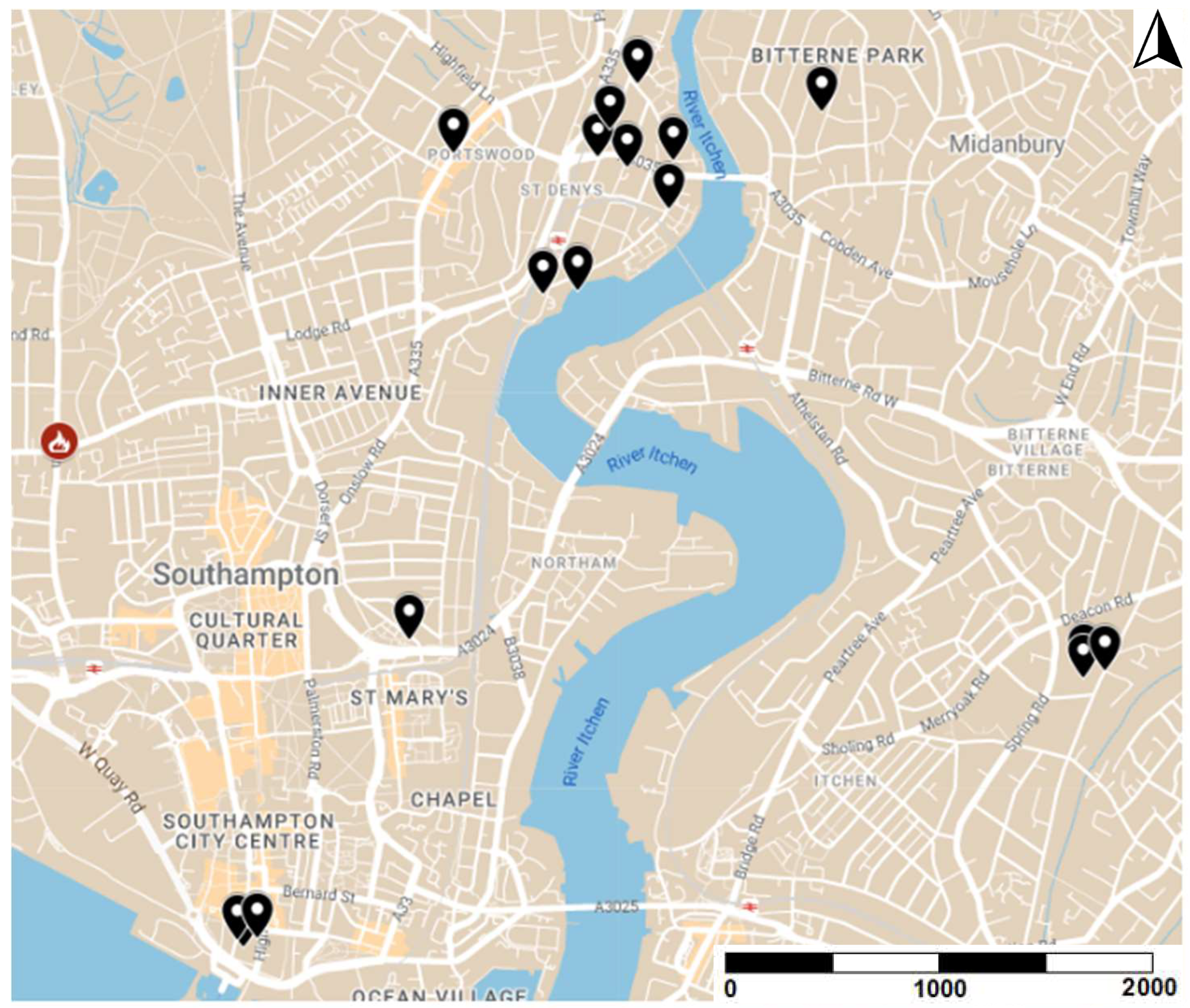
Figure 1. Location of low-cost sensors (black markers) across Southampton along with fire location (red marker). The smoke plume from the fire was captured primarily by the sensor located near St Mary’s, southeast of the source of the fire.
Atmosphere 15 01089 g001
Figure 2. Time series of wind speed and wind gust speed. Time = 0 denotes fire start time, corresponding to local time 17:30.
Atmosphere 15 01089 g002
Figure 3. Same as in Figure 2, but for wind direction.
Atmosphere 15 01089 g003
Figure 4. Same as in Figure 2, but for air temperature.
Atmosphere 15 01089 g004
Figure 5. Comparison of PMS and SPS sensor data showing consistency in monitored concentrations of PM2.5.
Atmosphere 15 01089 g005
Figure 6. CFD domain with a size of 3450 m (streamwise, x coordinate) × 2200 m (spanwise, y coordinate) × 1000 m (vertical, z coordinate). The streamwise direction is from the 310° wind direction (north-westerly wind).
Atmosphere 15 01089 g006
Figure 7. Mesh visualized on a plane within the city domain for zoomed-in near the St. Mary’s Football Stadium at ground level (left) and overview of mesh on the ground and far-field (right).
Atmosphere 15 01089 g007
Figure 8. CFD simulated instantaneous streamwise velocity (m/s).
Atmosphere 15 01089 g008
Figure 9. Sensor data downstream of fire with respect to the estimated fire start time (a) and zoomed-in for the duration of fire (b). The left side scale presents the measurements in units of μg/m3, whereas the right side scale presents the measurements non-dimensionalized based on an estimated emission rate Q = 50 g/s, the reference velocity U r e f , and the average building height h to aid the comparison in Section 5.3.
Atmosphere 15 01089 g009
Figure 10. Contours of ground level PM2.5 concentration at T = 1.5 h for a source temperature 500° with an emission rate 50 g/s, calculated from ADMS and presented over a wide domain in (a) and zoomed in close to the sensor in (b).
Atmosphere 15 01089 g010
Figure 11. Dimensionless emission rates for various source release periods.
Atmosphere 15 01089 g011
Figure 12. Dimensionless concentration at the sensor location from four CFD releases, compared with the sensor data. These are based on the estimated emission rate Q = 50 g/s, the freestream velocity U r e f , and the averaged building height h.
Atmosphere 15 01089 g012
Figure 13. Instantaneous concentration C / Q contours on ground level at 1.5 (top) and 3 (bottom) hours time after the fire started, provided by LES in OpenFOAM with an 80-min release. The streamwise direction was the incoming wind direction from left to right.
Atmosphere 15 01089 g013
Figure 14. Dimensionless concentration ( c ^ = C U r e f h 2 / Q ) time series. Sensor measurements normalized by three guessed emission rates: 5 g/s, 50 g/s and 150 g/s. Three fire temperatures tested in ADMS: 100 °C, 500 °C and 1000 °C. Two sample locations tested in OpenFOAM (OF): sensor site, and plume center.
Atmosphere 15 01089 g014
Figure 15. A comparison of the mean concentrations obtained from all three methods (sensors, CFD and ADMS) along with error bars representing the total uncertainty associated with each method and their associated assumptions.
Atmosphere 15 01089 g015
Figure 16. Concentration time series from sensor measurements, CFD and ADMS predictions, based on an estimated emission rate of 50 g/s (see Figure 14). Different fire temperatures 100 °C, 500 °C and 1000 °C were tested for the ADMS data.
Atmosphere 15 01089 g016
Table 1. A summary of the advantages, limitations and potential applications of the Gaussian plume model (GPM) and the large-eddy simulation (LES) for prediction of pollutant dispersion from an urban fire.
LESGPM
Spatial resolution (m)110
Temporal resolution (s)13600
Complexity in setupComplexSimple
Wind speed and directionYesYes
Wind vertical profiles, etc.YesNo
Considering ABL stabilityYes but not hereYes
Considering fire buoyancyYes but not hereYes
User experience levelExperienced CFD userEasy to use
Comput. cost (CPU hrs.)O(104)O(10−1)
Efficiency (wall-clock mins.)60 (Supercomputer)1 (Personal computer)
Output data dimensions3D in space & 1D in time2D in space
Output concentrationMean & flucts., plume extentMean, plume extent
Potential apps. (now)Support parameterizationFast predict. for
for GPM improvementscenarios as this case
Potential apps. (future)Fast predict. with supercomp.Improved fast predict.
Disclaimer/Publisher’s Note: The statements, opinions and data contained in all publications are solely those of the individual author(s) and contributor(s) and not of MDPI and/or the editor(s). MDPI and/or the editor(s) disclaim responsibility for any injury to people or property resulting from any ideas, methods, instructions or products referred to in the content.