Article

Stability Detection of Canopy RGB Images for Different Underlying Surfaces Based on SVM

1
Guangxi Zhuang Autonomous Region Meteorological Technology Equipment Center, Nanning 530022, China
2
Guangxi Institute of Meteorological Sciences, Nanning 530022, China
*
Author to whom correspondence should be addressed.
Atmosphere 2024, 15(8), 943; https://doi.org/10.3390/atmos15080943
Submission received: 3 June 2024 / Revised: 27 July 2024 / Accepted: 31 July 2024 / Published: 6 August 2024
(This article belongs to the Section Atmospheric Techniques, Instruments, and Modeling)

Abstract

:
This study aims to investigate the impact of different environmental conditions on the stability of RGB images in ecological sites and the anti-interference properties of vegetation images on different underlying surfaces. Three vegetation types including sugarcane, forest, and karst (mainly shrub and grass) are used to segment green vegetation using machine learning, and the RGB vegetation indices are calculated using color channel data. Then, The effect of weather, season, and time period on different types of vegetation indices are studied, which provide technical references for quantitative application of RGB image data. The results indicate the following: ① For the vegetation with high canopy density, the SVM machine learning segmentation algorithm used in this study is more applicable, as the RGB image segmentation accuracy of sugarcane and forest is significantly higher than karst. For different weather conditions, the segmentation accuracy of sugarcane and forest RGB images on sunny or cloudy days is higher than that on rainy or foggy days, but the effect on sparse vegetation in karst is not obvious. Additionally, the segmentation accuracy of different vegetation types has a small increase with NLM filter processing. ② Change in weather, season, and time can affect the stability of the image index. For different weather conditions, the vegetation indices of sugarcane and forest images on sunny or cloudy days are the more stable (ExGR, outlier proportion between 3.25% and 5.63%), while on rainy and foggy days they are less stable (ExR, outlier proportion between 17.60% and 21.59%). For different seasons, the stability of the sugarcane and karst image index obtained in spring is better (ExG, outlier proportion between 3.32% and 6.88%), while the stability of the forest image index obtained in summer is better (ExR, outlier proportion = 10.32%). For different times within a day, the sugarcane image index obtained in the morning is more stable (ExGR, outlier proportion = 4.62%), while the stability of the forest image index obtained in the afternoon is better (ExGR, outlier proportion = 9.24%). ③ The stability of the sugarcane image index is more affected by weather and season. For forest, the influence of the weather is more obvious than the season. But, for karst, the effect of season on the vegetation index is greater than that of weather.

1. Introduction

Guangxi has abundant forest and grass resources and is also a key distribution area of karst landforms in China, making its ecological location particularly important [1], 2023. Therefore, establishing a long-term ecological observation network has become an indispensable means and an inevitable trend in ecological research [2]. At present, Guangxi has established ecological observation stations covering various underlying surfaces, such as farmland, forests, and rocky deserts. Through long-term sequential positioning, continuous observation data acquisition, regular cognition, and other research, it plays an important role in the development of ecosystem-related fields [1]. Ecological observation stations belong to near-ground remote sensing and serve as a complement to satellite and drone remote sensing. The ecological stations carry RGB cameras with higher spatial resolution, enabling them to capture more detailed information about the vegetation canopy compared to satellite and drone remote sensing. And the long-term series observation system of the ecological station can track and observe the whole fertility period of vegetation, which can reflect the characteristics and laws of plants over time [3,4,5,6,7]. Because the ecological meteorological station collects vegetation information at a fixed location and at a fixed time, the images obtained in bad weather are susceptible to the effects of atmospheric particulate matter, resulting in degrading changes in the collected images and weakening the key information of visual effect and detail [8,9,10,11]. The images captured under complex weather conditions bring greater challenges to subsequent scientific research and analysis tasks [12].
Image segmentation is divided into uniform areas with specific semantic labels according to different internal characteristics in the image [13]. A vegetation image usually contains complex background noise. The segmentation of vegetation for research and analysis is conducive to improving the accuracy of analysis and inversion and is the basis for high-precision monitoring of vegetation [14]. As a hot topic in the field of computer vision, image segmentation has received increasing attention in the field of scientific research. RGB image-based segmentation technology methods have emerged one after another, and segmentation accuracy is also constantly improving, such as feature space clustering, histogram thresholding, and edge detection [15,16,17,18,19]; these segmentation techniques based on image color parameter features have been gradually explored by researchers, and their segmentation accuracy is also improving. With the rise of machine learning algorithms, a growing number of scholars are integrating machine learning algorithms into image segmentation techniques.
Near-ground RGB image remote sensing observations are susceptible to external conditions such as weather, season, light, and soil background [20,21], resulting in lower image stability and a higher dependence of image quality on light [22,23], which not only reduces the accuracy of image segmentation of ground objects but also reduces the stability of RGB image quality. Additionally, vegetation image quality is influenced by the underlying surface type, and there have been no reports on the impact of different external conditions on image stability. Therefore, this study takes the three vegetation cushion surfaces of sugarcane farmland, forest, and karst as its research object. Using the vegetation canopy segmentation images of the long-term RGB series from the ecological station, it analyses and compares the color spatial data stability of different underlying surfaces and uses the data of each channel for the following purposes: to calculate the RGB vegetation index; to analyze the stability of the vegetation index under the influence of different weather, seasons, and periods; and to provide a technical reference for the application of RGB image data from the canopy layer of the vegetation ecological stations.

2. Data and Methods

2.1. Overview of the Ecological Station

The sugarcane ecological meteorological observation station is located in Zhongdong Town, Fusui County, Chongzuo City, Guangxi (N 107°46′33.6″, E 22°51′57.6″). The forest ecological meteorological observation station is located in Zhongliang Township, Jinxiu County, Laibin City, Guangxi (N 110°14′45.6″, E 24°11′20.4″). The karst ecological meteorological observation station is located in Guohua Town, Pingguo County, Baise City, Guangxi (N 107°23′20.4″, E 23°23′27.6″). The observation equipment for the three observation stations is provided by Henan Zhongyuan photoelectric measurement and control technology Company, China. All three sites are in the subtropical monsoon climate zone, characterized by concurrent rainy and warm seasons. The vegetation types represent most of the vegetation in Guangxi, and as such they are relatively representative.

2.2. Data Source

2.2.1. Site Data

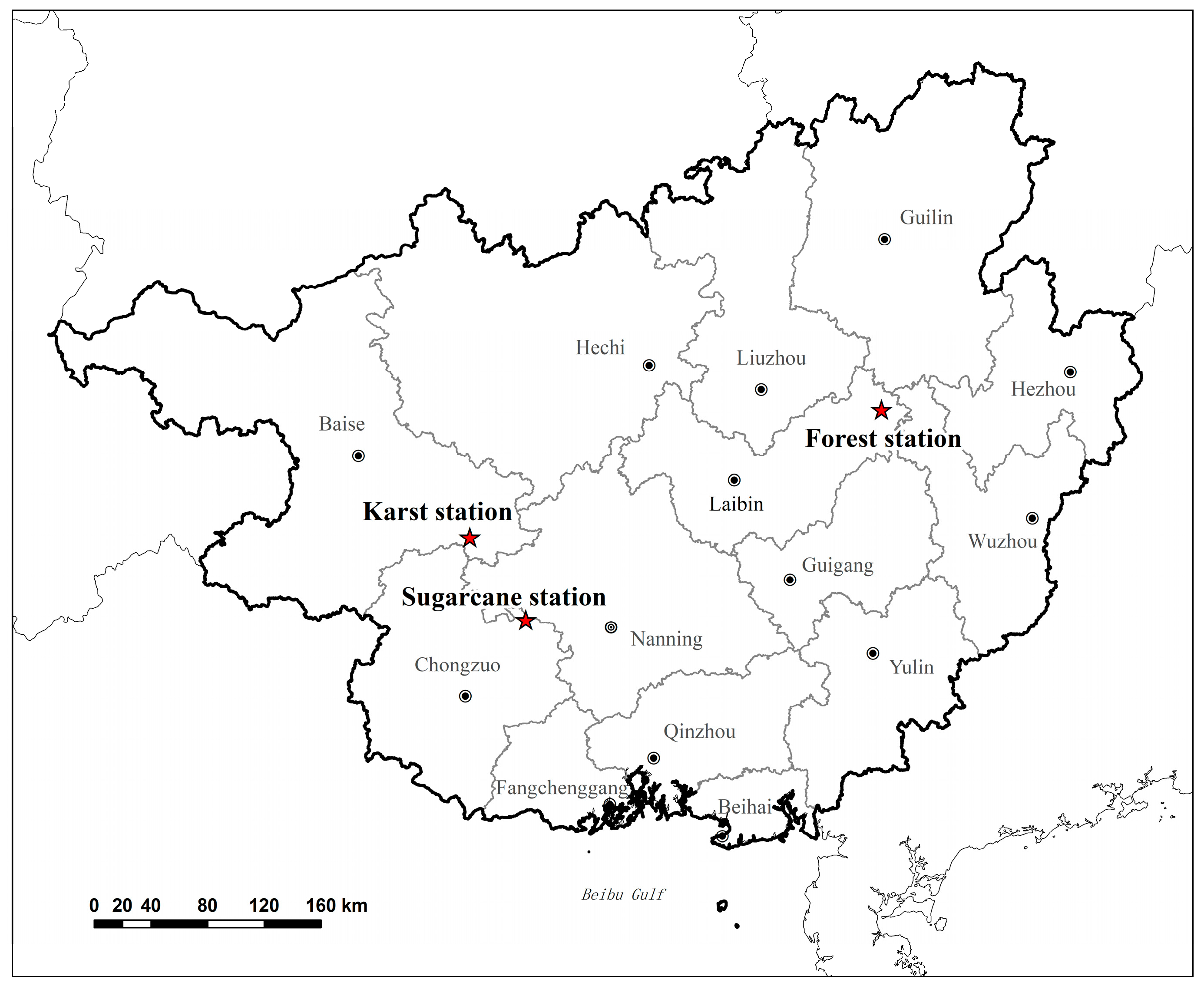
To control variables, the camera perspectives at the sugarcane ecological station, forest ecological station, and karst ecological station were all selected to be close-angle (approximately 45° with the ground), with long-term continuous image data. The observation areas are shown in Figure 1, and the distribution of sites is shown in Figure 2. The camera automatically captures images of the vegetation canopy at 8:00, 10:00, 12:00, 14:00, and 16:00 daily. The detailed image time series is provided in Table 1.

2.2.2. Meteorological Data

Meteorological data are provided by the Guangxi Zhuang Autonomous Region Meteorological Bureau, including hourly rainfall and types of weather processes. The criteria of weather classification is shown in Table 2.

2.3. Research Method

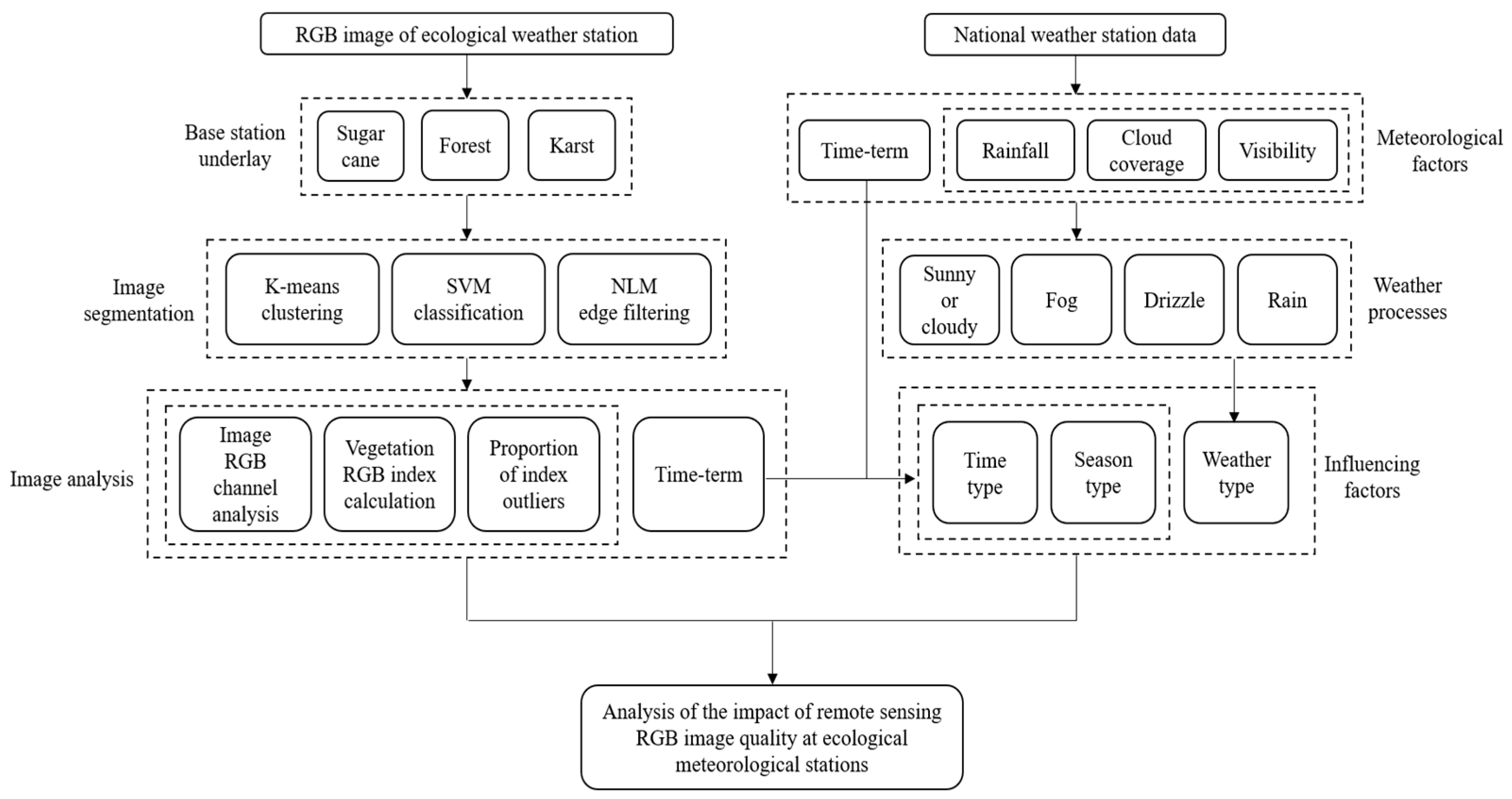
The flow chart of the research methodology of this study is shown in Figure 3. In this study, machine learning was used to separate the vegetation and background of the image. The image index was calculated based on the separated vegetation images. The partial correlation analysis between image index and different weather, season and time period was carried out to explore the influencing factors of image quality stability.

2.3.1. Image Segmentation

This study uses machine learning segmentation algorithms. Firstly, K-means unsupervised clustering is used to generate training samples and then filtered. Then, the Support Vector Machine (SVM) is used to classify plants and soil backgrounds. To reduce phenomena such as missed detections and false detections, the segmented images are further optimized through Non-Local Means (NLM) filtering, which eliminates misjudged areas at the edges of segmented images.
  • K-means algorithm
The K-means algorithm is an unsupervised partition clustering algorithm which uses distance as the similarity evaluation index, and the closer the distance between two objects, the greater the similarity. For a given dataset (x) with (n) objects (x) = {x1, x2, x3, …, xn}), each of which has the attributes of (m) dimensions, (n) objects are finally clustered into a specified (k) cluster according to the similarity between the objects, each of which only belongs to one clustered class, and the object is the smallest distance from the center of the cluster. The steps to implement the Gram–Mearns algorithm are as follows [24]:
Firstly, initialize the clustering center, which has a number of (k): {c1, c2, c3, … , ck }, 1 < kn;
Secondly, calculate the Euclidean distance from each object to each cluster center:
d x , c i = j = 1 d x j c i j 2
where (x) represents the data point, (ci) represents the (i)th clustering center, (d) represents the dimension of the data, and (xj) and (cij) represent the values of (x) and (ci) in the (j)th dimension, respectively.
Thirdly, investigate the distance from each object to each cluster center and divide the objects into clusters with the closest cluster center to obtain clusters which have a number of (k):{S1, S2, S3, …, Sk}.
Fourthly, for each cluster, calculate the average of all data points, taking that average as the new center point:
c i = 1 S i x S i x
Finally, repeat the assignment and update the steps until the clustering center no longer changes significantly, and then terminate the condition.
2.
SVM
SVM is a supervised learning model for classification and regression analysis. It determines the optimal classification by calculating the optimization problem so that it can handle complex data classification problems [25,26,27].
Firstly, select the most suitable SVM kernel function. The kernel function used in this paper is the radial basis kernel function, and the expression is as follows:
K x i , x j = exp g x i x j 2 , g > 0
where (g) represents the tunable parameter that controls the width of the RBF nucleus, and x i x j represents the Euclidean distance between the two data points (xi) and (xj).
After that, the kernel function is substituted into the SVM image for classification. The expression of the SVM optimal classification function is as follows [28]:
S x = s i g n i = 1 n a i y i K x i , x j + b
where (ai) represents the non-negative Lagrange multiplier, (yi) represents the category, K (xi,yi) represents the kernel function, and (b) is the classification threshold.
3.
NLM filtering
NLM filtering is a classic image denoising algorithm based on repetitive local structures in the image. It removes noise by using weighted averaging of similar pixels, which better preserves image details. The denoised images also exhibit relatively high clarity, making this method widely applicable in practice [29]. Its principle is as follows [30]:
Firstly, let I = { I ( x , y ) | x , y S } be the noisy image. The denoised image is obtained by taking the weighted average of the other pixels in O ( x , y ) .
O i , j = x , y ω x , y I x , y
The core of the Non-Local Means algorithm is to compute the similarity weight coefficients using the Euclidean distance ω x , y to quantify the similarity between image blocks. The Euclidean distance d ( x , y ) between the pixel point (y) in the search window and the central pixel point (x) is given by
d x , y = | V x V y | W 2
where V ( x ) and V ( y ) represent the grayscale values of the similar image blocks, with ( x ) and ( y ) as the center pixel points, respectively, within the search window; (W) is the side length of the similar window.
Secondly, the similarity weight coefficients can be obtained from the Euclidean distance ω ( x , y ) between pixel points, given by
ω x , y = 1 M x e x p d x , y h 2
where (h) is the filtering coefficient, and M ( x ) is the normalization coefficient, with the mathematical expression given by
M x = y = L d x , y h 2
where (L) is the side length of the search window.
Finally, accuracy assessment is conducted on the segmented image using manually annotated results as references. The formulas for accuracy assessment metrics (Qseg) and (Sr) are as follows [31]:
Q s e g = i = 0 i   =   m j   =   0 j   =   m A p i j B p i j i = 0 i = m j   =   0 j   =   m A p i j B p i j
S r = i   = 0 i   = m j   = 0 j   = m A p i j B p i j i   = 0 i   = m j   = 0 j   = m B p i j
where (A) represents the pixel set of foreground (green vegetation) or background (information outside green vegetation) after segmentation; (p = 255) for foreground and (p = 0) for background); (B) denotes the manually obtained pixel set of foreground (p = 255) or background (p = 0); (m) and (n) are the numbers of rows and columns of the image, respectively; (i) and (j) are the corresponding coordinates; larger values of (Qseg) and (Sr) indicate higher segmentation accuracy, where (Qseg) indicates the overall consistency between segmented background and foreground, and (Sr) only represents the consistency of foreground segmentation results.

2.3.2. RGB Vegetation Index Calculation and Correlation with Weather, Season, and Time Period Conditions

Calculation of vegetation index: extract the RGB color-space data of the green vegetation region in the image after segmentation and calculate the RGB vegetation index according to the formula in Table 3.
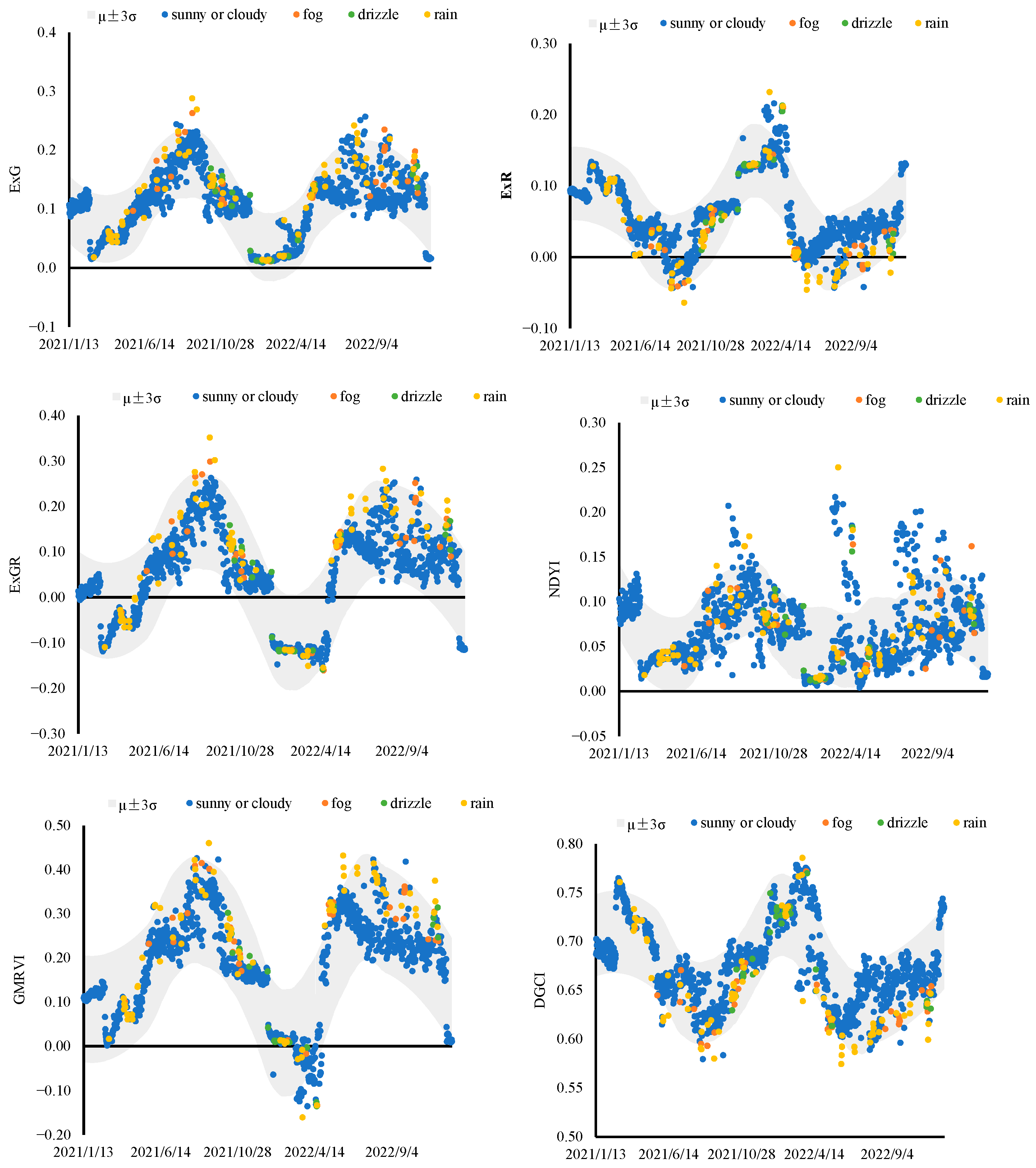
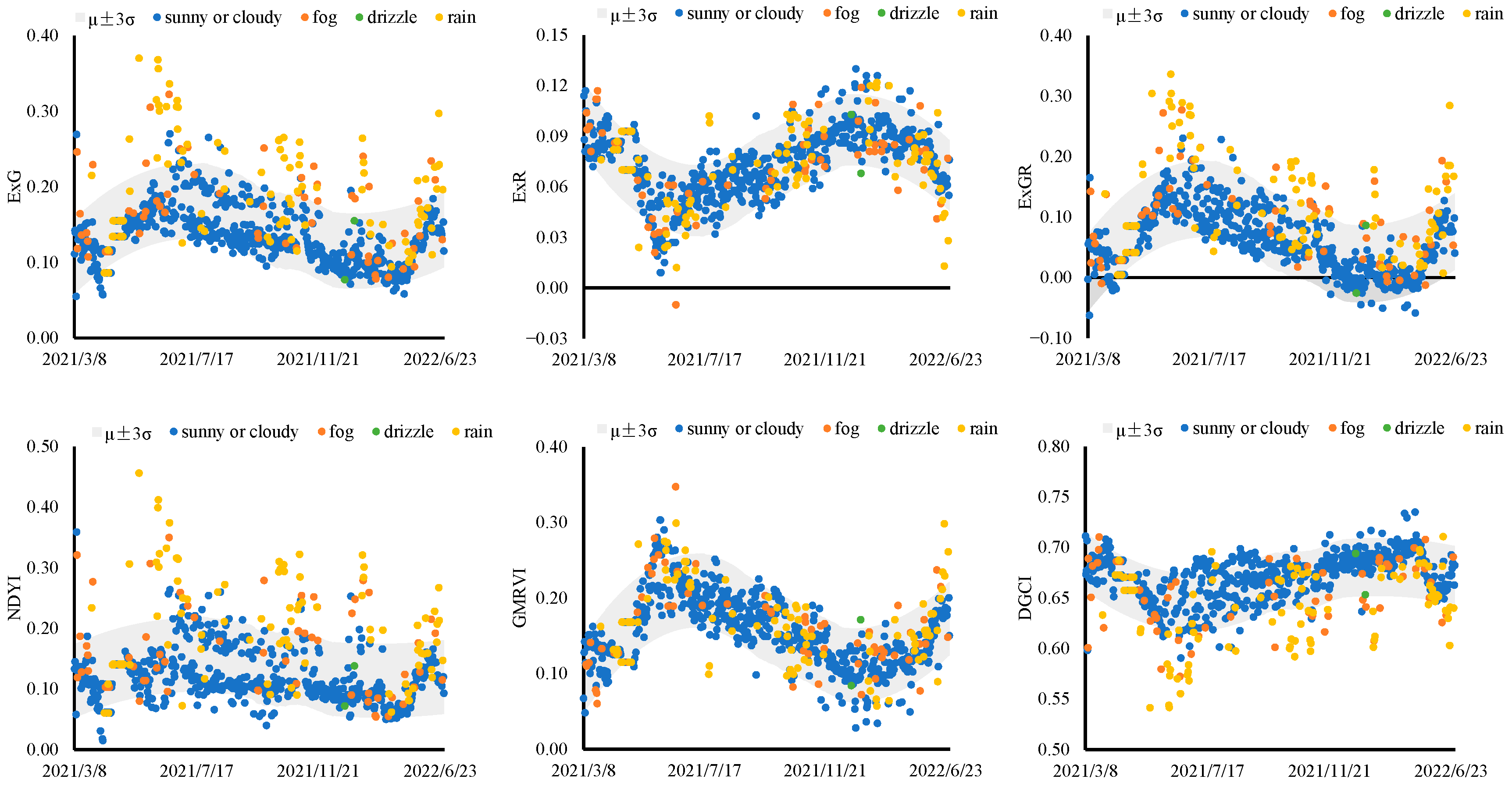
Determination of outlier values of vegetation index: Outliers are identified according to the 3RMS criterion; the control limit interval (μ − 3σ, μ + 3σ) was constructed by taking 3σ as the control limits, and the premise is that the measurement time series follows a normal distribution. Data within the interval are defined as normal, while data outside the interval are defined as outliers [38]. Due to the significant seasonal fluctuation in the actual vegetation index of the image, the 100-day moving average value of vegetation index is used as the reference value μ, and the 100-day moving average value of the standard deviation is used as the σ.
Correlation between vegetation index, weather, season, and time period: Using SPSS25, partial correlation analysis was conducted on the vegetation index under different weather, season, and time period conditions. Partial correlation analysis can eliminate the correlation between two variables, and its calculation formula is as follows [39]:
R x y · z = R x y R x z × R y z 1 R x z 2 + 1 R y z 2
In the formula, Rxy·z is the partial correlation coefficient between x and y after the variable z is fixed. Rxy is the correlation coefficient between x and y, Rxz is the correlation coefficient between x and z, and Ryz is the correlation coefficient between y and z.

3. Result Analysis

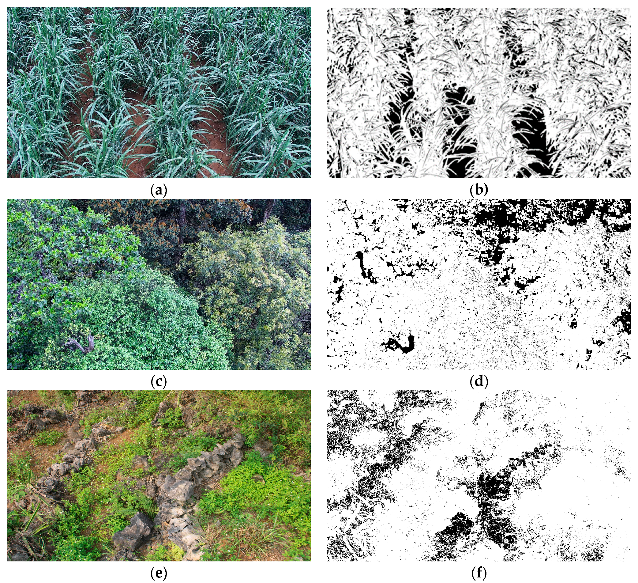
To maintain data consistency and reliability, vegetation segmentation images taken during the summer and autumn seasons, when plant growth is lush and lighting is stable (between 10 am and 12 pm), were used for horizontal comparison analysis. Figure 4 and Table 4 indicate that SVM has a high degree of distinction for high-coverage vegetation, such as sugarcane and forest. For example, the sugarcane site’s Qseg reached 80.64%, and Sr reached 82.81%, both being the highest among all means. However, for bare rocks, the differentiation is lower, with a mean Qseg and Sr of 78.67% and 80.01%, respectively. Therefore, the segmentation effect of SVM is related to the level of vegetation cover on the underlying surface, and the segmentation effect of bare rock is significantly lower than that of high-coverage vegetation.
The image segmentation effects of each underlying surface are different under different weather conditions (Table 4). Under sunny or cloudy conditions, SVM exhibits significantly higher segmentation accuracy for agricultural fields and forest underlying surface images, exceeding that of rainy or foggy days by 5.83% to 7.97%. Conversely, for karst underlying surfaces, the segmentation accuracy under sunny or cloudy conditions is slightly lower than that under rainy or foggy conditions, by 2.79% to 4.23%. The impact of different weather conditions on the segmentation accuracy of underlying surfaces with higher vegetation cover is more pronounced, but there is no significant impact on bare rock underlying surfaces. The standard deviation of Qseg for sugarcane and forest sites under different weather conditions ranges from 3.98% to 2.74%, and Sr ranges from 3.43% to 4.12%, respectively, higher than that of karst sites by 0.48% to 1.72% and 2.27% to 2.95%. The segmentation effect of SVM is affected by weather conditions, but different underlying surfaces have different sensitivities to the effects of weather conditions.
NLM filtering can effectively optimize various segmentation results, and the segmentation accuracy of leaf edge and background is slightly improved after filtering (Table 4). The segmentation accuracy of each station increased after filtering, and the mean Qseg and Sr of the sugarcane station increased by 0.62% and 0.68%, respectively; the Qseg and Sr of the forest station increased by 0.72% and 0.80%, respectively; and the Qseg and Sr of the karst station increased by 0.66% and 0.67%, respectively. The filtering effect of the ecological station on the three underlying surfaces showed consistency under different weather conditions: the filtering effect of the images without weather processes (sunny or cloudy) was better than that of images with weather processes (fog, rain, and drizzle).

3.1. Image RGB Channel Analysis

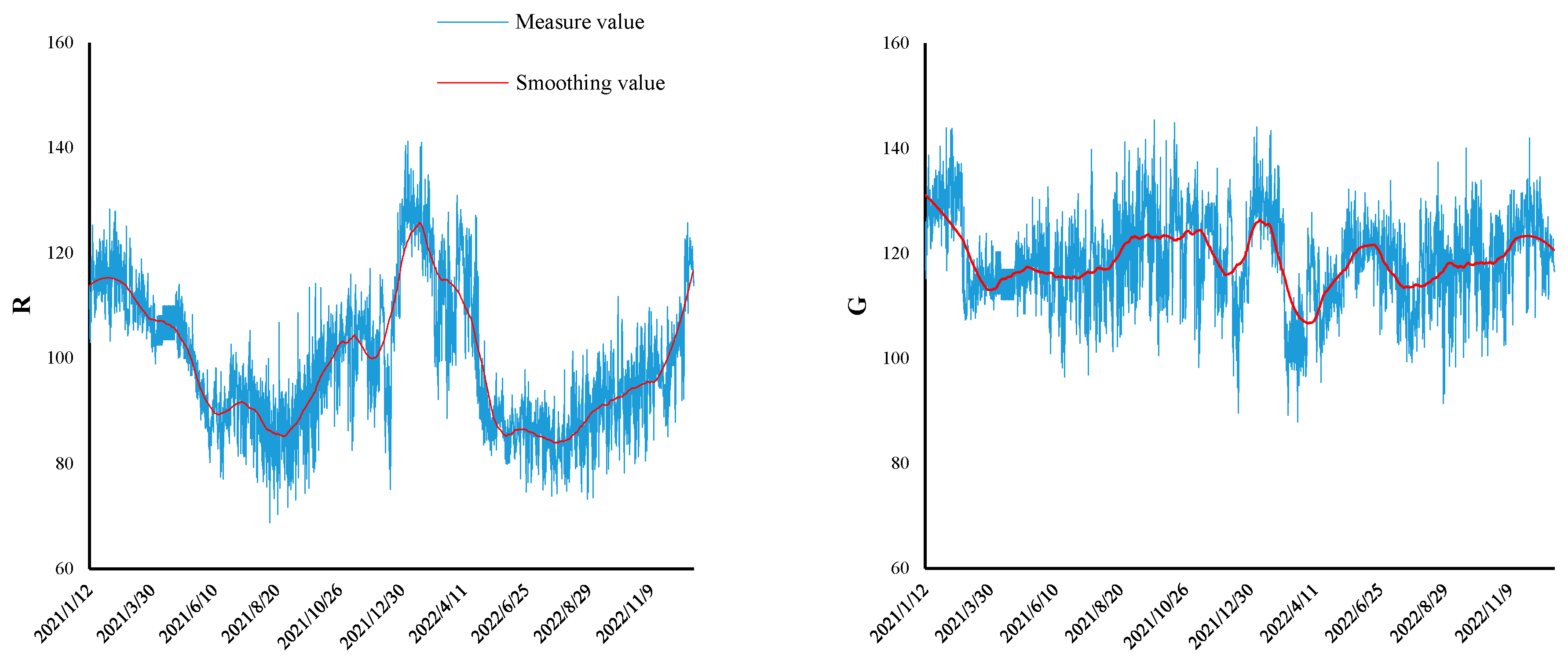
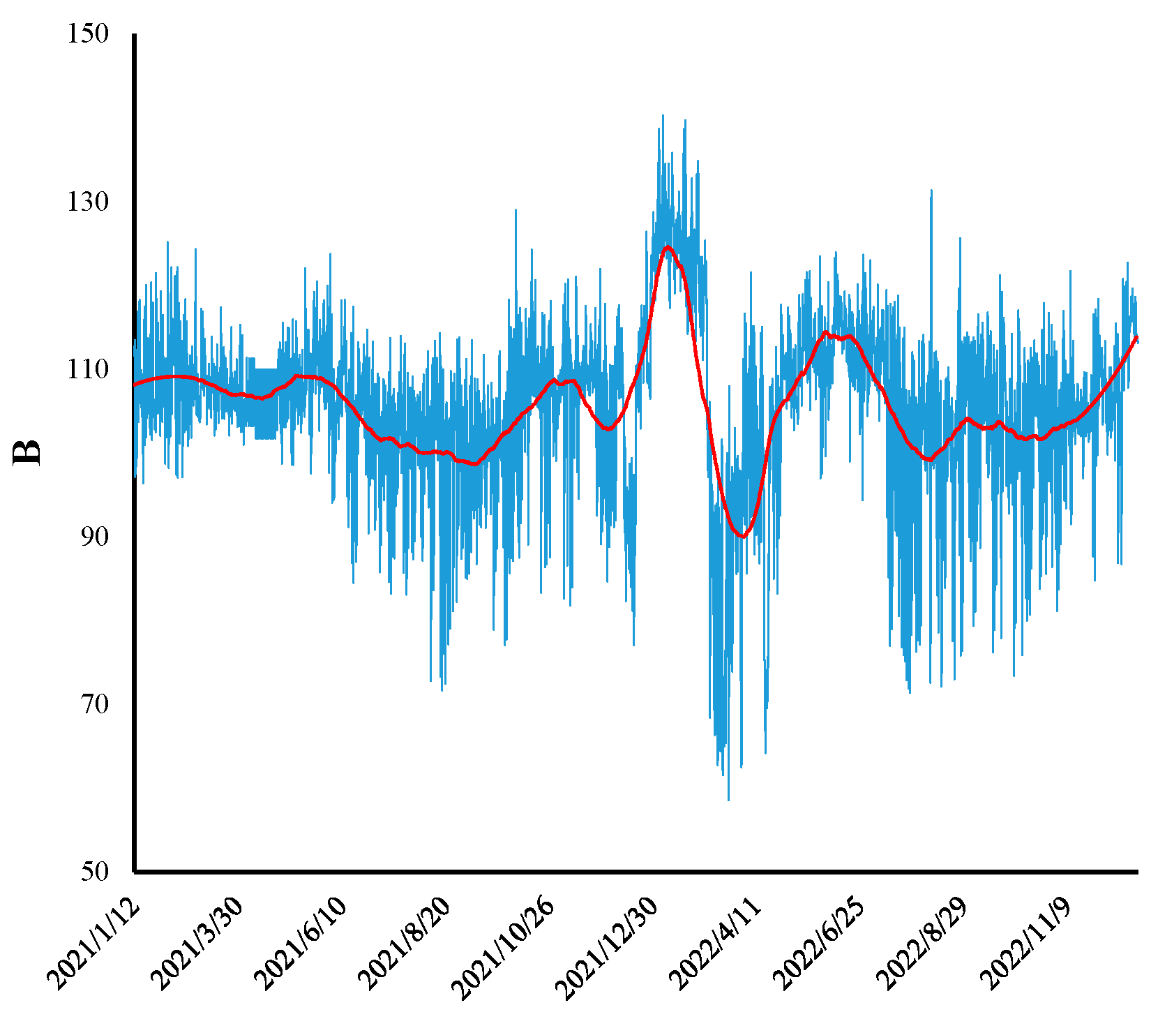
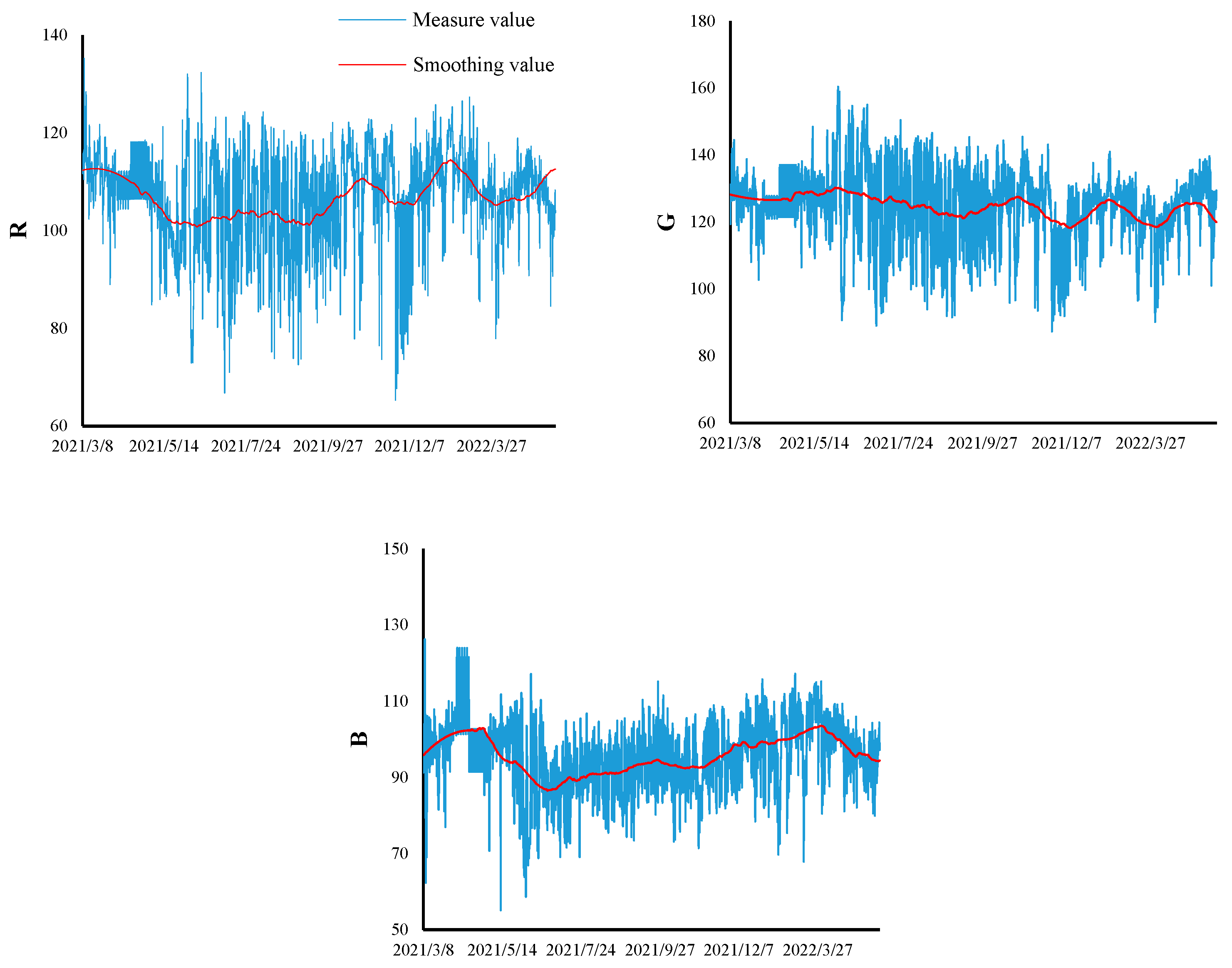
Compared with the long-term series change of the three color-space channel data of the three types of underlying surface ecological station RGB images (Figure 5, Figure 6 and Figure 7), it can be observed that the sugarcane station’s image data exhibit strong fluctuations, showing a relatively regular seasonal variation. The data dispersion of each channel falls between that of the forest station and the karst station. The seasonal fluctuation of the karst station data is weak; the dispersion of each channel is the smallest, the forest site has no obvious seasonality, and the dispersion of each channel is the largest.
The RGB pixel values of sugarcane and forest underlying surface images satisfy G > R > B, indicating that the green channel has the highest reflectance, followed by the red channel, and finally the blue channel, which conforms to the spectral variation law of green vegetation. The RGB pixel value ordering of karst images is G ≈ R > B, indicating that the RGB images of the ecological stations can distinguish between vegetation and non-vegetation (naked soil, cement, etc.) underlying surfaces.

3.2. Analysis of the Influence of the Image Vegetation Index and Different External Conditions

3.2.1. Weather Type

Analysis of vegetation indices at different ecological stations under various weather conditions was conducted using data from 10 to 12 o’clock. Figure 8, Figure 9 and Figure 10 reveal significant differences in the dispersion of vegetation indices at ecological stations under different weather conditions. For the sugarcane image, except for NDYI, the proportion of outlier values for vegetation indices is noticeably higher on foggy, light rain, and rainy days compared to sunny or cloudy days. The proportion of outlier values for indices on rainy days is generally higher than other weather types, reaching up to 22.08%, followed by foggy and light rain days, with most vegetation indices’ outlier values exceeding 15%. For the forest image, the proportion of outlier values for vegetation indices is consistently the highest on foggy days, ranging from 18.75% to 35.94% overall. For the karst image, the proportion of outlier values for vegetation indices on foggy, light rain, and rainy days is slightly higher than on sunny or cloudy days, with foggy days consistently having the highest proportion of outlier values for vegetation indices. However, the difference in the impact of different weather conditions on the proportion of outlier values for most vegetation indices is not significant. Thus, it can be observed that rainy days have the greatest impact on the stability of vegetation indices for sugarcane images, with the stability of vegetation indices significantly lower during weather processes than on sunny or cloudy days. Foggy days have the greatest impact on the stability of vegetation indices for forest and karst images, but for karst images, the occurrence of weather processes does not significantly impact the stability of vegetation indices.

3.2.2. Seasonal Type

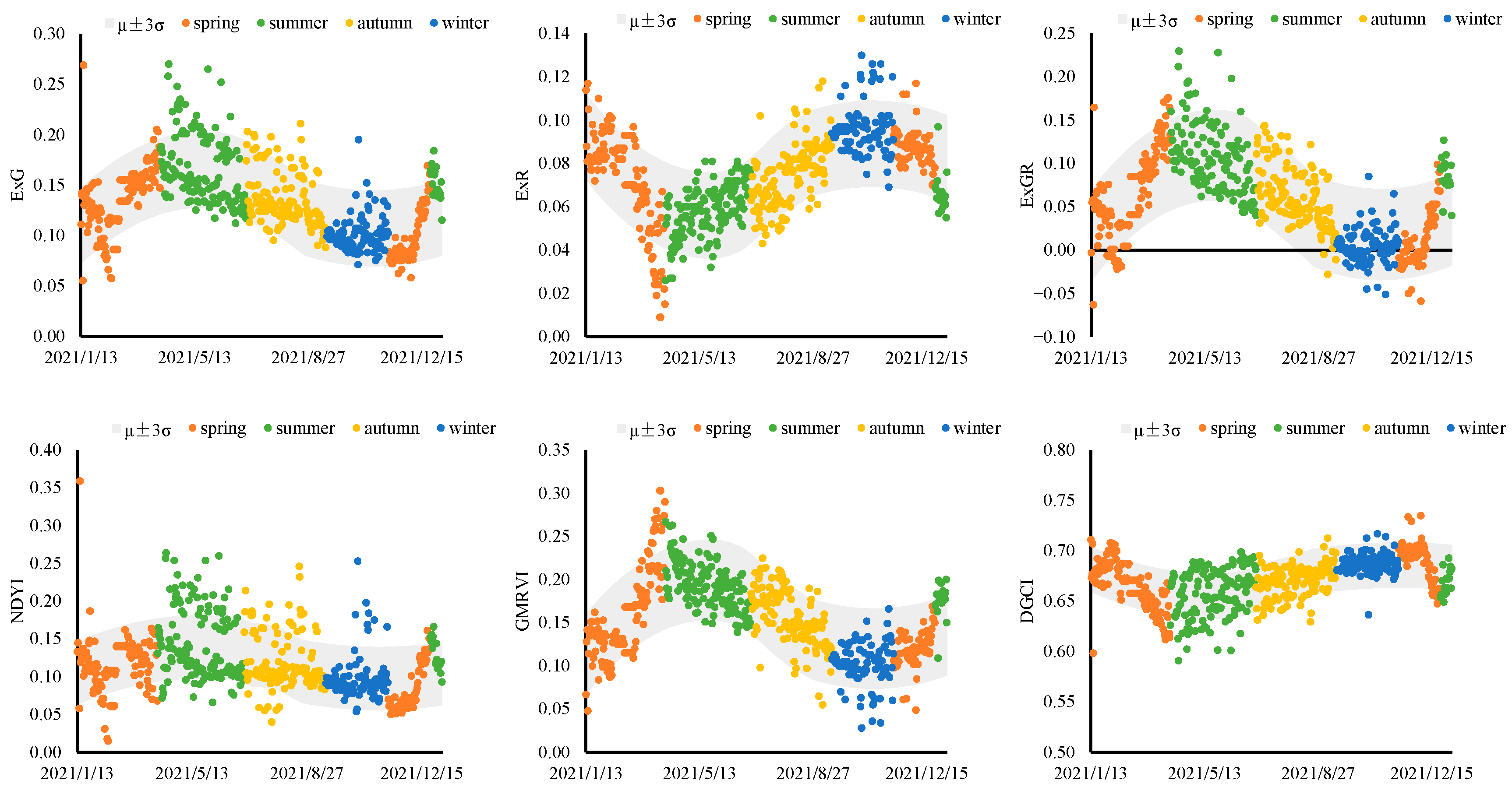
Figure 11, Figure 12 and Figure 13 reveal significant differences in the dispersion of various vegetation indices for different land covers across different seasons. For the sugarcane image, the proportions for ExR, GMRVI, and DGCI out-of-group values in spring are significantly higher than in other seasons, of which the DGCI vegetation index accounts for as much as 31.73%. Vegetation indices in summer, autumn, and winter are relatively stable, and only the index out-of-group values for NDYI are relatively high. For the forest image, the outlier proportions for vegetation indices are high in spring and summer, with over half of the indices having outlier proportions exceeding 20% in summer. Autumn follows with outlier proportions ranging from 9.38% to 21.88%, while winter shows the most stable vegetation indices, with only NDYI exceeding 5%. For the karst image, except for DGCI, outlier proportions for various vegetation indices are higher in spring compared to winter, with differences ranging from 6.88% to 10.62%. This indicates that spring has the greatest impact on the stability of sugarcane and karst images, while summer has the greatest impact on the stability of forest images. Winter has the least impact on the stability of images for all three land covers.

3.2.3. Timeline Type

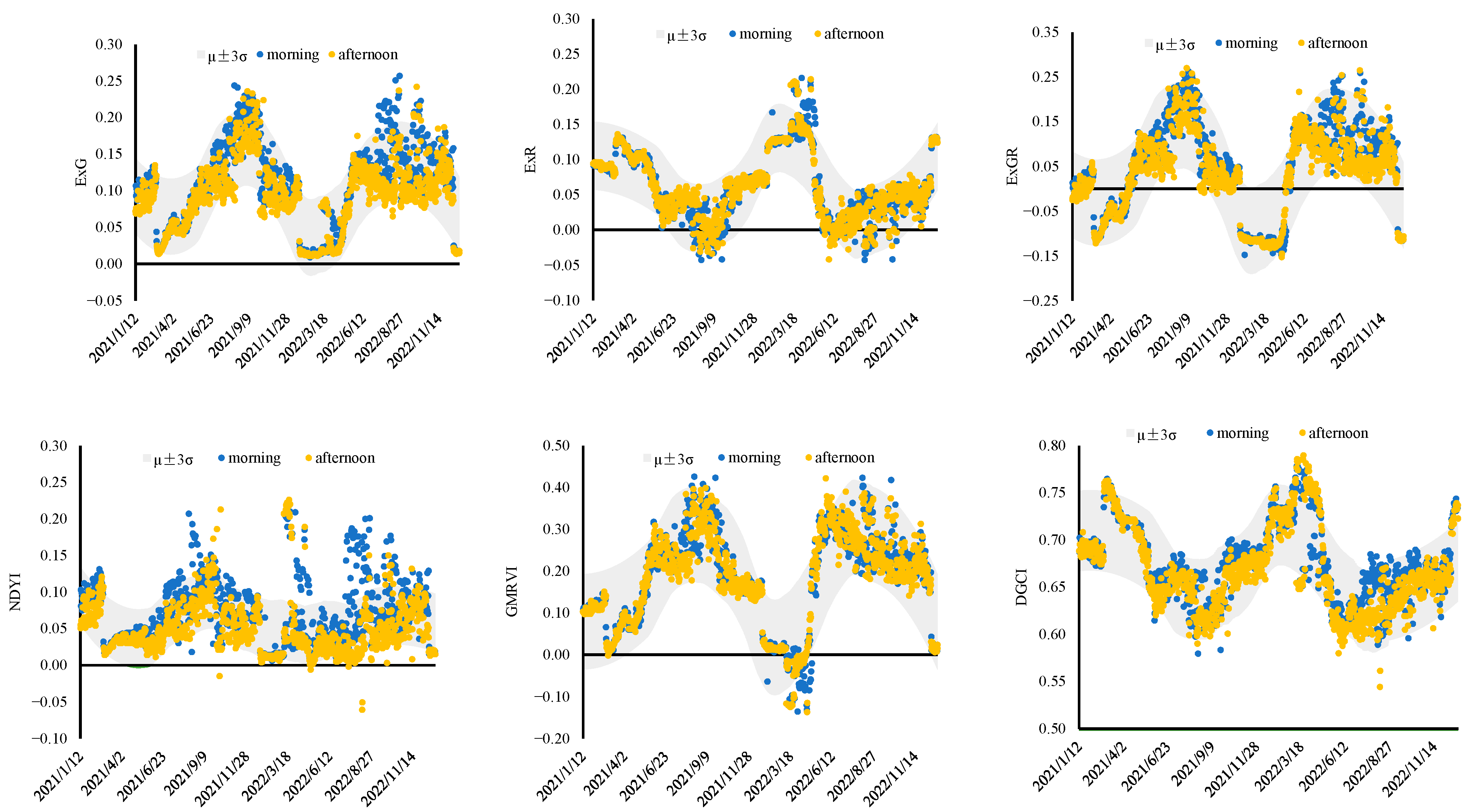
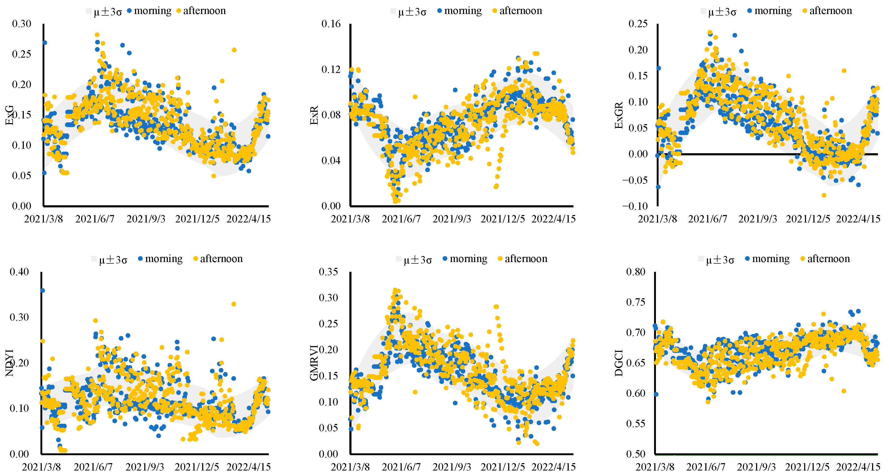
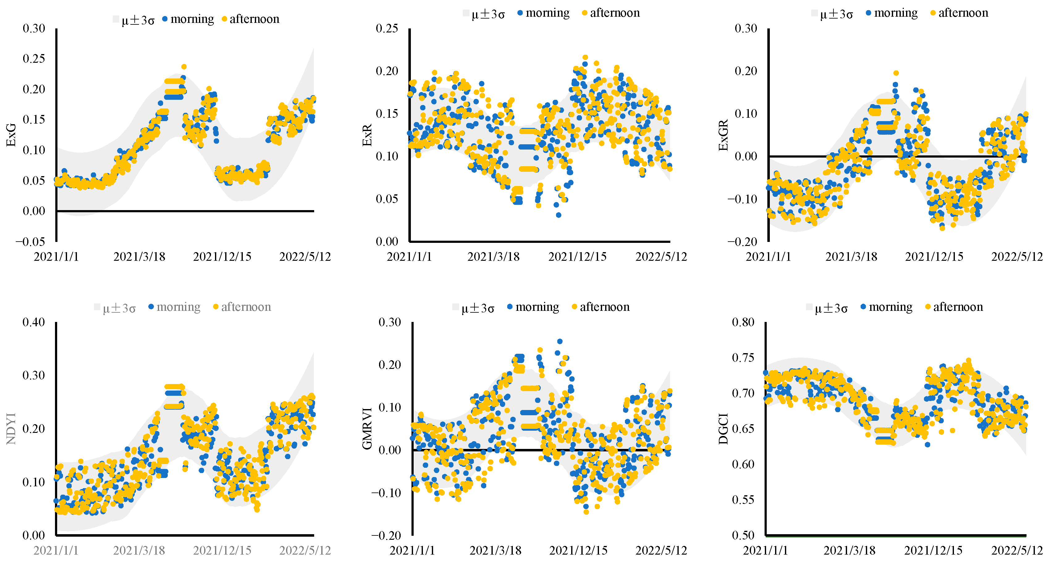
The different shooting periods have an impact on the stability of vegetation images from the ecological stations. As depicted in Figure 14, Figure 15 and Figure 16, the majority of vegetation index outliers at the sugarcane stations captured during the morning period exceed those in the afternoon; however, they generally remain small, with most vegetation index outlier proportions being less than 15%. For the forest stations, the proportion of outlier values in the vegetation index images during the morning period is generally lower than in the afternoon period, with both NDYI and DGCI outlier proportions exceeding 15%. Similar to the forest stations, the karst stations exhibit a higher proportion of vegetation index outliers during the afternoon period compared to the morning period, with outlier proportions generally higher than those of the forest stations; notably, ExG and GMRVI exhibit the highest outlier proportions, at 28.81% and 22.33%, respectively. In comparison, the differences in vegetation index outlier proportions between morning and afternoon images for the three types of underlying surfaces are relatively small, ranging from 0.60% to 5.11%. Consequently, it can be observed that the morning period has a greater impact on the stability of sugarcane images, while the opposite is true for forest and karst images. Nonetheless, the difference in vegetation index outlier rates between the two time periods is not significant.

3.3. Analysis of the Influence of the Image Vegetation Index and Different External Conditions

The partial correlation coefficients between different weather, seasons and time periods and the number of outliers in the vegetation index are shown in the Table 5. For sugarcane sites, there is a relatively high partial correlation between weather conditions, seasonal variations, and the number of outliers in vegetation index imagery. All probabilities of vegetation index outliers are significantly correlated with seasons (p < 0.05), with approximately half of the vegetation indices being highly significant (p < 0.01). The DGCI exhibits the highest correlation with seasonal types, with over half of the vegetation indices being extremely correlated with weather types, among which the ExGR coefficient is higher than that of other vegetation indices. For forest sites, different weather types show a high partial correlation with the probability of vegetation index outliers, and all vegetation indices are significantly correlated with weather types, with ExG exhibiting the highest correlation coefficient of 0.398. For karst sites, there is a strong partial correlation between seasonal variations and outliers in various vegetation index data. All vegetation indices are significantly correlated with seasons, with over half of them being significantly correlated. The correlation between the shooting period and the probability of vegetation index outliers for the three types of sites is relatively low, with the majority of vegetation indices showing no significant correlation with the period. It can be seen that changes in weather and seasons have a significant impact on the stability of vegetation indices in ecological sites, leading to a higher probability of outliers in vegetation indices due to weather and seasonal changes. Moreover, different underlying surfaces exhibit varying resistance to the influence of weather or seasons. Sugarcane imagery shows a higher probability of vegetation index outliers caused by weather and seasonal changes, while forest imagery is more affected by weather changes and less affected by seasonal changes. In contrast, karst imagery exhibits the opposite trend. Therefore, weather and seasonal changes have a greater impact on the stability of sugarcane imagery, while weather changes have a greater impact on forest imagery stability, and seasonal changes have a greater impact on karst imagery stability. The shooting period has a relatively small impact on the stability of imagery for all three types of sites.

4. Discussion

This study found that the segmentation performance of SVM is influenced by the underlying surface vegetation coverage. The composition of bare soil and rocks is complex, which often leads to instances of false positives and false negatives during image segmentation [40,41]. In this study, the K-means unsupervised clustering method was employed to generate training samples. After screening the samples, a support vector machine was used to classify vegetation and background information. Finally, the divided image was filtered by Non-Local Mean to remove the wrong edge pixels, which further improved the accuracy of classification. Guangxi belongs to the subtropical monsoon climate zone, with a warm climate and abundant rain. The spring and summer are humid and cloudy, resulting in the presence of clouds being observed on most of the sunny days. For that reason, the combination of sunny and cloudy was used in this study to compare with rain, fog, drizzle, and other weather. The accuracy of vegetation segmentation varies under different weather conditions. This may be due to a difference in the color saturation of the image taken due to the different intensity of sunlight on sunny or cloudy and rainy days. For sugarcane and forest, the light conditions on rainy and foggy days result in reduced vegetation color saturation, making it more prone to confusion with soil backgrounds [14]. For karst, the reflectivity of rocks is higher than that of soil, which causes an uneven color of the rocks in the images [42]. Also, the interference of shadows in bright light affects the accuracy of image segmentation, and the dimming of the light weakens the interference of highlights and shadows on image segmentation. The accuracy of the ecological station images is slightly increased after filtering, and the filtering effect is different under different weather conditions. However, the optimization effect of filtering on image segmentation is not significant.
The stability of ecological vegetation images varies significantly under different weather, seasonal, and time conditions. The deviation of the vegetation index in images caused by weather changes may be due to several factors. Firstly, rainy and foggy weather results in higher vegetation water content, leading to more pronounced color differences [43]. This, in turn, causes a substantial deviation in vegetation indices. Secondly, the obstruction of rain and fog can interfere with the camera’s accurate capture of vegetation morphology and color. The deviation in image vegetation indices affected by seasonal changes, which may be related to the seasonal growth of vegetation, are here significant differences in the different growth stages of plants, whether in agricultural fields or grasslands, which are reflected in the corresponding spectral image features [44]. This leads to significant differences in the discreteness of image vegetation indices in different seasons. The stability of vegetation indices varies at different shooting times, possibly because the differences in light conditions between morning and afternoon affect the camera’s exposure time, thereby influencing the quality of vegetation images [14].
The stability of vegetation images varies among different underlying surfaces in response to weather, season, and time of day. For sugarcane, the vegetation shows significant growth characteristics at different stages with seasonal change, resulting in obvious seasonal fluctuations. During spring, sugarcane is in the sprouting stage, characterized by rapid growth and low coverage of ground stems and leaves, leading to significant impacts on image stability. Some studies have also found that the spectral inversion effects of crops in the early stages of growth are generally unstable [45,46,47]. Concurrently, weather conditions also affect the images of crop ecological stations; rainfall or air humidity alters the underlying surface’s moisture content, which leads to the variation in spectral energy absorption, consequently influencing vegetation indices. In karst regions, vegetation mainly comprises grasslands and shrubs, which are highly sensitive to seasonal changes. During periods of rapid vegetation growth, and given the mountainous terrain of the karst ecological stations, the wind speed and direction change frequently, resulting in significant differences in the morphology and position of shrubby vegetation, leading to drastic changes in RGB image vegetation indices [14].
This study found that the occurrence of weather processes significantly impacts the image stability of forest stations, possibly due to the elevated position of the forest ecological stations above the forest canopy, which is much higher compared to the sugarcane and karst ecological stations, so the presence of raindrops and fog during rainy and foggy weather conditions may interfere more disruptively with the accurate collection of vegetation information in the camera images. For sugarcane stations, rainfall impacts the image quality by altering the moisture content of the vegetation and the soil, causing it to appear darker in the image. The vegetation on the underlying surface of the karst is sparse, mostly grass and shrubs, and there are more bare rocks, which have a low absorption rate of rainwater and little impact on image quality. Forest ecological stations observe predominantly evergreen vegetation types, which are less sensitive to seasonal changes, resulting in the minimal impact of seasons on image stability.
This study discusses the image stability of a long-term time series from ecological stations with different underlying surfaces from three perspectives: weather, season, and time period. However, it does not explore the impact of different camera perspectives on image stability, so we will further explore the correlation between the two areas in the future, and explore the influence of different camera perspectives on image index and image quality.

5. Conclusions

The image segmentation effect of SVM is related to the vegetation coverage of the underlying surface, and the segmentation effect of bare rock is significantly lower than high-coverage vegetation. Weather conditions also impact the segmentation performance, with sugarcane and forest images showing better segmentation on sunny or cloudy days, while karst images exhibit better segmentation during rainy or foggy conditions. The underlying surface with higher vegetation coverage is more sensitive to different weather conditions, while the underlying surface with bare rock is less sensitive. The accuracy of the images of each ecological station is slightly increased after filtering.
Rainy days have a significant impact on the stability of sugarcane vegetation indices, while foggy conditions affect the stability of forest and karst vegetation indices. However, the occurrence of weather processes has a less pronounced effect on the stability of vegetation indices for karst images. Spring has a notable impact on the stability of sugarcane and karst vegetation indices, while summer affects the stability of forest vegetation indices. The influence of morning on the stability of the sugarcane vegetation index is stronger than that of afternoon, whereas the opposite is observed for forest and karst vegetation indices, although the difference in stability between the two time periods is minimal.
Weather and seasonal changes have a greater impact on the stability of sugarcane images, while weather variations predominantly affect the stability of forest images, and seasonal changes have a more pronounced effect on the stability of karst images. The shooting time period has a minor impact on the image stability of all three underlying surfaces.

Author Contributions

Conceptualization, Y.C.; methodology, Y.C. and W.T.; software, L.H. and K.J.; validation, W.T. and Y.C.; formal analysis, W.T.; investigation, W.T. and Z.C.; resources, K.J. and Z.C. data curation, Z.C. and K.J.; writing—original draft preparation, W.T. and L.H.; writing—review and editing, Z.C. and Y.C.; visualization, W.T. and L.H.; supervision, Y.C. and W.T.; project administration, Y.C.; funding acquisition, Y.C. All authors have read and agreed to the published version of the manuscript.

Funding

The research was supported by the key Research and Development Project of the Science and Technology Department of the Guangxi Zhuang Autonomous Region (Guike AB20159022 & AB21238010).

Institutional Review Board Statement

Not applicable.

Informed Consent Statement

Not applicable.

Data Availability Statement

The data presented in this study are available on request from the corresponding author. The data are not publicly available due to future publications.

Acknowledgments

Thanks to the Meteorological Bureau of Guangxi Zhuang Autonomous Region for its support and assistance in building ecological stations.

Conflicts of Interest

We declare no conflicts of interest.

References

  1. Lu, F.; Cai, H.D.; Su, H.X.; Tong, D.W.; Liang, Y.Y.; Qin, Z.W.; Luo, W.S. The construction of Guangxi Region terrestrial ecosystem positioning observation research network. Hunan For. Sci. Technol. 2023, 50, 75–82. [Google Scholar]
  2. Zhang, F.H.; Zhang, Y. Strengthen the linkage of ecosystem positioning and observation networks to help Inner Mongolia develop green and high-quality. Inn. Mong. For. 2022, 10, 8–9. [Google Scholar]
  3. Tian, S.; Wei, B.; Jin, H.; Liu, Y.; Liu, F.; Yin, P.; Jia, B. Soil Properties and Hydrological Indexes of Forest Stands in Xuexiang. For. By-Prod. Spec. China 2023, 6, 7–8+12. [Google Scholar] [CrossRef]
  4. Chang, Q.Q.; He, H.L.; Niu, Z.E.; Ren, X.L.; Zhang, L.; Sun, W.X.; Zhu, X.B. Spatio-temporal variation of soil moisture and its influencing factors in Chinese typical forest ecosystems. Acta Ecol. Sin. 2021, 41, 490–502. [Google Scholar]
  5. Chen, R.F.; Yang, H.Y.; Gao, X.H.; Zheng, Z.L. Analysis of Microclimate Characteristics in Xiaolongshan Forest Ecological Station Area. J. Gansu For. Sci. Technol. 2019, 44, 5–8. [Google Scholar]
  6. Wang, X.Y.; Chen, Y.Q.; Xue, C.W.; Lin, Z.P.; Su, S.F.; Xue, Y. Analysis of Main Nutrient Contents in Leaves of Plants around Wenchang Ecological Station of Hainan. J. Anhui Agric. Sci. 2017, 45, 170–171+197. [Google Scholar]
  7. Yang, N.; Zhou, M.; Chen, H.; Cao, C.; Du, S.; Huang, Z. Estimation of Wheat Leaf Area Index and Yield Based on UAV RGB Images. J. Triticeae Crops 2023, 43, 920–932. [Google Scholar]
  8. Gu, H.C. Research on Foggy Image Sharpening Method Based on Dark Channel. Master’s Thesis, Shenyang Ligong University, Shenyang, China, 2023. [Google Scholar]
  9. Narasimhan, S.G.; Nayar, S.K. Chromatic Framework for Vision in Bad Weather. In Proceedings of the IEEE Conference on Computer Vision and Pattern Recognition, CVPR 2000, Hilton Head, SC, USA, 15 June 2000; IEEE: Piscataway, NJ, USA, 2000; pp. 598–605. [Google Scholar]
  10. McCartney, E.J. Optics of the Atmosphere: Scattering by Molecules and Particles. Phys. Today 1977, 30, 76–77. [Google Scholar] [CrossRef]
  11. Narasimhan, S.G.; Nayar, S.K. Vision and the Atmosphere. Int. J. Comput. Vis. 2002, 48, 233–254. [Google Scholar] [CrossRef]
  12. Wang, H.; Zhang, Y.; Shen, H.H.; Zhang, J.Z. A review of image enhancement algorithms. Chin. Opt. 2017, 10, 438–448. [Google Scholar] [CrossRef]
  13. Min, L.; Gao, K.; Li, W.; Wang, H.; Li, T.; Wu, Q. A Review of the Optical Remote Sensing Image Segmentation Technology. Spacecr. Recovery Remote Sens. 2020, 41, 1–13. [Google Scholar]
  14. Chen, Y.L.; Fang, S.B.; Mo, J.F.; Liu, Z.P. Characteristic of Typical Vegetation Growth in Karst Area based on Ground-based Visible Images. Remote Sens. Technol. Appl. 2023, 38, 518–526. [Google Scholar]
  15. Liu, S.Y.; Li, L.; Te, R.; Li, Z.; Ma, J.; Zhu, R. Threshold segmentation algorithm based on histogram region growing for remote sensing images. Bull. Surv. Mapp. 2021, 2, 25–29. [Google Scholar]
  16. Chen, L.; Ding, G.H.; Guo, L. Image thresholding based on mutual recognition of histogram. J. Infrared Millim. Waves 2011, 30, 80–84. [Google Scholar] [CrossRef]
  17. Li, J.; Jiang, N.; Baoyin, B.; Zhang, F.; Zhang, W.J.; Wang, W. Spatial Color Clustering Algorithm and Its Application in Image Feature Extraction. J. Jilin Univ. Sci. Ed. 2020, 58, 627–633. [Google Scholar]
  18. Ren, J.; Li, Z.N.; Fu, Y.P. Edge detection of color images based on wavelet and reduced dimensionality model of RGB. J. Zhejiang Univ. Eng. Sci. 2004, 38, 856–859, 892. [Google Scholar]
  19. Ma, X.; Qi, L.; Zhang, X.C. Segmentation Technology of Exserochilum Turcicum Image Based on Fuzzy Clustering Analysis. J. Agric. Mech. Res. 2008, 12, 24–26. [Google Scholar]
  20. Yu, N.; Li, L.; Schmitz, N.; Tian, L.F.; Greenberg, J.A.; Diers, B.W. Development of methods to improve soybean yield estimation and predict plant maturity with an unmanned aerial vehicle based platform. Remote Sens. Environ. 2016, 187, 91–101. [Google Scholar] [CrossRef]
  21. Ma, Y.P.; Bian, M.B.; Fan, Y.G.; Chen, Z.C.; Yang, G.J.; Feng, H.K. Estimation of Potassium Content in Potato Leaves Based on Canopy Spectrum and Coverage. Trans. Chin. Soc. Agric. Mach. 2023, 54, 226–233+252. [Google Scholar]
  22. Wang, C.Y.; Guo, X.Y.; Wen, W.L.; Du, J.J.; Xiao, B.X. Application of hemispherical photography on analysis of maize canopy structural parameters under natural light. Trans. Chin. Soc. Agric. Eng. 2016, 32, 157–162. [Google Scholar]
  23. You, M.; Liu, J.; Zhang, J.; Xv, M.; He, D. A novel chicken meat quality evaluation method based on color card localization and color correction. IEEE Access 2020, 8, 170093–170100. [Google Scholar] [CrossRef]
  24. Yang, J.C.; Zhao, C. Survey on K-Means clustering algorithm. Comput. Eng. Appl. 2019, 55, 7–14. [Google Scholar]
  25. Mazzoni, D.; Garay, M.J.; Davies, R.; Nelson, D. An Operational MISR Pixel Classifier Using Support Vector Machines. Remote Sens. Environ. 2007, 107, 149–158. [Google Scholar] [CrossRef]
  26. Zhang, R.; Ma, J.W. New progress in the application of support vector machines in remote sensing data classification. Adv. Earth Sci. 2009, 24, 555–562. [Google Scholar]
  27. Long, Y.F.; Qiao, W.Y.; Sun, J. Change Detection of Remote Sensing Images in Datun Mining Area Based on Support Vector Machine. Geomat. Spat. Inf. Technol. 2020, 43, 107–110. [Google Scholar]
  28. He, L.J. Research on Weeds Identification Based on K-Means Feature Learning. Master’s Thesis, Northwest A&F University, Xianyang, China, 2016. [Google Scholar]
  29. Li, L.H.; Guo, H.F.; Yu, P.; Liu, L.; Lu, X.H. Improved Non-Local Means Filtering Algorithm of Mine Remote Monitoring Image. Met. Mine 2022, 10, 165–169. [Google Scholar]
  30. Qi, W.; Jia, C.X.; Li, J. Application of Improved Non-local Mean Filtering in Image Denoising. J. Taiyuan Univ. (Nat. Sci. Ed.) 2023, 41, 59–64. [Google Scholar] [CrossRef]
  31. Guo, W.; Rage, K.U.; Ninomiya, S. Illumination invariant segmentation of vegetation for time series wheat images based on decision tree model. Comput. Electron. Agric. 2013, 96, 58–66. [Google Scholar] [CrossRef]
  32. Woebbecke, D.M.; Meyer, G.E.; Von Bargen, K.; Mortensen, D.A. Colour indices for weed identification under various soil, residue, and lighting conditions. Trans. ASAE 1995, 38, 259–269. [Google Scholar] [CrossRef]
  33. Meyer, E.G.; Neto, C.J. Verification of colour vegetation indices for automated crop imaging applications. Comput. Electron. Agric. 2008, 63, 282–293. [Google Scholar] [CrossRef]
  34. Guijarro, M.; Pajares, G.; Riomoros, I.; Herrera, P.; Burgos-Artizzu, X.; Ribeiro, A. Automatic segmentation of relevant textures in agricultural images. Comput. Electron. Agric. 2010, 75, 75–83. [Google Scholar] [CrossRef]
  35. Sulik, J.J.; Long, D.S. Spectral Considerations for Modeling Yield of Canola. Remote Sens. Environ. 2016, 184, 161–174. [Google Scholar] [CrossRef]
  36. Bendig, J.; Yu, K.; Aasen, H.; Bolten, A.; Bennertz, S.; Broscheit, J.; Gnyp, M.L.; Bareth, G. Combining UAV-based plant height from crop surface models, visible, and near infrared vegetation indices for biomass monitoring in barley. Int. J. Appl. Earth Obs. Geoinf. 2015, 39, 79–87. [Google Scholar] [CrossRef]
  37. Douglas, E.K.; Michael, D.R. Quantifying Turfgrass Colour Using Digital Image Analysis. Crop Sci. 2003, 43, 943–951. [Google Scholar]
  38. Wu, H.; Wang, S.Y. Abnormal Data Recognition Algorithm for GNSS Deformation Monitoring Based on Laida Criterion. Sci-Tech Innov. Product. 2019, 1, 30–34. [Google Scholar] [CrossRef]
  39. Wu, H.; Bai, J.; Li, J.L.; Jiapaer, G.; Bao, A.M. Study of spatio-temporal variation in fractional vegetation cover and its influencing factors in Xinjiang, China. Chin. J. Plant Ecol. 2024, 48, 41–55. [Google Scholar]
  40. Garía-Mateos, G.; Hernández-Hernández, J.L.; Escarabajal-Henarejos, D.; Jaén-Terrones, S.; Molina-Martínez, J.M. Study and comparison of color models for automatic image analysis in irrigation management applications. Agric. Water Manag. 2015, 151, 158–166. [Google Scholar] [CrossRef]
  41. Jin, F.J. Research on Feature Extraction and Recognition Method of Weed Image Based on Machine Vision. Ph.D. Thesis, Zhenjiang Jiangsu University, Zhenjiang, China, 2007. [Google Scholar]
  42. Chen, L.J. Research on Image Enhancement Algorithm in Complex Weather Environment. Master’s Thesis, Xiamen University, Xiamen, China, 2022. [Google Scholar] [CrossRef]
  43. Yang, C.; Zhan, P.; He, L.; Hu, W.; Wei, Y. Visual detection of moisture content of mulberry leaf based on hyperspectral imaging technology. Acta Sericol. Sin. 2023, 49, 430–437. [Google Scholar] [CrossRef]
  44. Li, G.S.; Liu, J.B.; Liu, P.G.; Zhao, C.J.; Zhang, B.; Tong, Q.X. Analysis on Influence of Seasonal Changes and Terrain Undulation on Image Matching Guidance. Radio Eng. 2010, 12, 27–30. [Google Scholar]
  45. Liu, L.Y.; Wang, J.H.; Huang, W.J.; Zhao, C.J. Improving winter wheat yield prediction by novel spectral index. Trans. Chin. Soc. Agric. Eng. 2004, 20, 172–175. [Google Scholar]
  46. Jia, K.L.; Zhang, J.H. Prediction of the salinity information of Takyr Solonetzs based on the spectral characteristics of rice Canopy Indexes. Chin. J. Soil Sci. 2012, 43, 281–285. [Google Scholar]
  47. Ma, Y.P.; Bian, M.B.; Fan, Y.G.; Chen, Z.; Yang, G.; Feng, H. Estimation of potassium content in potato plants based on UAV RGB images. Trans. Chin. Soc. Agric. Mach. 2023, 54, 196–203. [Google Scholar]
Figure 1. Ecological station perspectives. (a) Sugarcane ecological station, (b) forest ecological station, (c) karst ecological station.
Atmosphere 15 00943 g001
Figure 2. Distribution of ecological meteorological stations.
Atmosphere 15 00943 g002
Figure 3. Technical flow chart.
Atmosphere 15 00943 g003
Figure 4. Comparison of effects before and after RGB canopy image segmentation of ecological stations. (a) Image of the sugarcane station before segmentation. (b) Image of the sugarcane station after segmentation. (c) Forest station image before segmentation. (d) Forest station image after segmentation. (e) Karst station image before segmentation. (f) Karst station image after segmentation.
Atmosphere 15 00943 g004
Figure 5. Sugarcane canopy RGB image color space channel time series change.
Atmosphere 15 00943 g005aAtmosphere 15 00943 g005b
Figure 6. Forest canopy RGB image color space channel time series change.
Atmosphere 15 00943 g006
Figure 7. Karst canopy RGB image color space channel time series change.
Atmosphere 15 00943 g007
Figure 8. Discrete distribution of the sugarcane canopy image vegetation index.
Atmosphere 15 00943 g008
Figure 9. Discrete distribution of the forest canopy image vegetation index.
Atmosphere 15 00943 g009
Figure 10. Discrete distribution of the karst canopy image vegetation index.
Atmosphere 15 00943 g010
Figure 11. Discrete distribution of the sugarcane canopy image vegetation index.
Atmosphere 15 00943 g011
Figure 12. Discrete distribution of the forest canopy image vegetation index.
Atmosphere 15 00943 g012
Figure 13. Discrete distribution of the karst canopy image vegetation index.
Atmosphere 15 00943 g013aAtmosphere 15 00943 g013b
Figure 14. Discrete distribution of the sugarcane cane canopy image vegetation index.
Atmosphere 15 00943 g014
Figure 15. Discrete distribution of the forest canopy image vegetation index.
Atmosphere 15 00943 g015
Figure 16. Discrete distribution of the karst canopy image vegetation index.
Atmosphere 15 00943 g016
Table 1. Ecological station image collection time series.
Ecological StationTime
Sugarcane12 January 2020–31 December 2022
Forest8 March 2021–30 June 2022
Karst1 January 2021–31 May 2021, 4 November 2021–20 May 2022
Table 2. Criteria of weather classification.
WeatherRainfall (mm)Cloud Cover ExtentVisibility (m)
Sunny or cloudy<1Covers less than half of the sky>15,000
Rain>20Cover more than half of the sky1000–5000
Drizzle10~20Cover more than half of the sky5000–15,000
Fog1~10Cover more than half of the sky<500
Table 3. RGB Vegetation index.
Vegetation IndexCalculation FormulaSource
ExG2grb[32]
ExR1.4rg[33]
ExGRExG − 1.4rg[34]
NDYI(gb)/(g + b)[35]
MGRVI(g2r2)/(g2 + r2)[36]
DGCI[(HUE−60)/60 + (1 − S) + (1 − B)]/3[37]
Note: r, g, and b represent the three spectral channels of the RGB color space, while HUE, S, and B represent hue, saturation, and brightness, respectively.
Table 4. Ecological Station RGB Crown Image Segmentation Accuracy.
Base StationIndexWeather Condition
Sunny or
Cloudy
FoggyDrizzleRainyAverageStandard
Deviation
SugarcaneBefore
filtering
Qseg84.01%74.87%83.24%77.94%80.02%3.78%
Sr86.98%76.35%85.06%80.12%82.13%4.17%
After
filtering
Qseg84.89%75.24%83.98%78.43%80.64%3.98%
Sr87.66%77.11%85.62%80.83%82.81%4.12%
ForestBefore
filtering
Qseg82.63%75.01%78.90%80.20%79.19%2.76%
Sr86.70%78.12%80.36%84.89%82.52%3.43%
After
filtering
Qseg83.35%75.77%79.65%80.86%79.91%2.74%
Sr87.65%78.94%81.19%85.48%83.32%3.43%
KarstBefore
filtering
Qseg75.48%76.11%79.99%80.45%78.01%2.23%
Sr77.73%78.79%80.70%80.11%78.33%2.33%
After
filtering
Qseg76.14%76.71%80.68%81.13%78.67%2.25%
Sr78.32%79.58%81.37%80.75%80.01%1.17%
Table 5. The partial correlation coefficient between different weather, seasons, and periods and the number of vegetation indices.
ExGExRExGRNDYIGMRVIDGCI
SugarcaneWeather classification0.105 **0.138 **0.153 **−0.0020.120 **0.025
Season classification0.047 *−0.080 **0.047 *−0.051 *−0.060 **−0.172 **
Time classification0.009−0.043 *0.031−0.025−0.041 *0.009
ForestWeather classification0.398 **0.087 **0.395 **0.328 **0.118 **0.274 **
Season classification0.0080.106 **0.0020.0320.0350.014
Time classification−0.0310.087 **−0.0480.0120.083 **−0.052 *
KarstWeather classification−0.005−0.057−0.051−0.009−0.065−0.097 **
Season classification−0.105 **−0.115 **−0.141 **−0.073 *−0.110 **0.084 *
Time classification−0.024−0.035−0.017−0.018−0.0150.042
Note: ** is p < 0.01, * is p < 0.05.
Disclaimer/Publisher’s Note: The statements, opinions and data contained in all publications are solely those of the individual author(s) and contributor(s) and not of MDPI and/or the editor(s). MDPI and/or the editor(s) disclaim responsibility for any injury to people or property resulting from any ideas, methods, instructions or products referred to in the content.