Article

PT-ESM: A Parameter-Testing and Integration Framework for Earth System Models Oriented towards High-Performance Computing

College of Computer Science and Technology, Jilin University, Changchun 130012, China
*
Author to whom correspondence should be addressed.
Atmosphere 2024, 15(8), 935; https://doi.org/10.3390/atmos15080935
Submission received: 18 June 2024 / Revised: 25 July 2024 / Accepted: 31 July 2024 / Published: 5 August 2024
(This article belongs to the Special Issue High-Performance Computing for Atmospheric Modeling)

Abstract

:
High-performance computing (HPC) plays a crucial role in scientific computing, and the efficient utilization of HPC to accomplish computational tasks remains a focal point of research. This study addresses the issue of parameter tuning for Earth system models by proposing a comprehensive solution based on the concept of scientific workflows. This solution encompasses detailed methods from sensitivity analysis to parameter tuning and incorporates various approaches to enhance result accuracy. We validated the reliability of our methods using five cases in the Single Column Atmosphere Model (SCAM). Specifically, we investigated the influence of fluctuations of 11 typical parameters on 10 output variables. The experimental results show that the magnitude of the impact on the results varies significantly when different parameters are perturbed. These findings will help researchers develop more reasonable parameterization schemes for different regions and seasons.

1. Introduction

High-performance computing (HPC) plays an important role in many fields, including climate simulation [1], molecular dynamics [2,3], earthquake simulation [4], and quantum computing [5]. Naturally, it has extensive and profound applications in the field of Earth sciences, providing scientists with powerful computational capabilities to simulate, analyze, and predict the complex behavior of the Earth system. Climate modeling is one of the important applications of HPC in the field of Earth sciences. By simulating the interactions of complex systems such as the atmosphere, oceans, and land, scientists can predict future climate change trends. HPC can handle large-scale climate datasets, simulate complex physical and chemical processes, and provide high-resolution climate change predictions. This is of great significance for formulating strategies to address climate change, assessing its potential impacts, and predicting the occurrence of natural disasters [6]. In the field of geological research, HPC is widely used for simulating earthquakes, plate movements, magma flows, and more. With HPC, scientists can model complex geological processes such as crustal movement and rock deformation, leading to a deeper understanding of Earth’s structure and evolution. Additionally, HPC can be employed for data processing in oil and gas exploration, helping scientists more accurately determine the location and scale of oil and gas reservoirs [7]. Ocean science research involves extensive data processing and simulation work. HPC offers powerful computational capabilities to support complex studies, including ocean circulation, wave dynamics, and marine ecosystem simulations. By leveraging HPC, scientists can gain deeper insights into the dynamic changes occurring in the ocean, providing critical scientific evidence for marine resource development and ocean environmental protection [8].
HPC also plays a crucial role in the field of environmental science. By simulating the dispersion processes of pollutants in the atmosphere, water bodies, and soil, scientists can assess the impact of pollution on the environment and develop effective pollution control measures [9]. Additionally, HPC can be used to simulate and analyze the dynamic changes of ecosystems, providing scientific evidence for ecological protection. In addition, there is another field that cannot be overlooked. Geographic Information Systems (GIS) [10] and remote sensing technology [11] are important tools in Earth science research. HPC can efficiently process large-scale geographic information and remote sensing data, providing fast and accurate data analysis and visualization results. This is of great significance for land resource management, urban planning, disaster monitoring, and other areas [12].
Earth system models (ESMs) in high-performance computing (HPC) are used to simulate and understand the complex interactions within the Earth’s climate system, including the atmosphere, oceans, land surface, and ice. These models are essential for predicting future climate scenarios, studying environmental changes, and guiding better policy decisions. However, there is considerable uncertainty in the parameters used in ESMs, which can affect the accuracy of simulations. Parameter tuning is an ongoing challenge that requires extensive validation and calibration against observational data. Although existing research has explored parameter uncertainty in models, there is often a lack of a comprehensive methodology for large-scale parameter experiments, which is insufficient for the computational power of HPC.
Therefore, in this paper, we propose PT-ESM, a high-performance computing (HPC)-oriented framework for parameter testing and integration in Earth system models. This framework effectively harnesses the powerful computational capabilities of HPC to assist in various experiments related to Earth system science. Building on this, we present practical scenarios of parameter testing using the Single Column Atmosphere Model (SCAM) and validate the usability of this framework.

2. Related Work

Scientific workflows have become essential tools in managing complex and large-scale computational tasks in various scientific domains [13]. These workflows automate and streamline the sequence of data processing steps, from data collection and preprocessing to analysis and visualization [14]. They enhance reproducibility, scalability, and efficiency in handling intricate computational tasks, particularly in high-performance computing (HPC) environments. Researchers are developing sophisticated tools and frameworks to automate the orchestration of scientific workflows. Tools like Apache Airflow [15], Pegasus [16], and Kepler [17] enable the automation of data processing pipelines, ensuring that tasks are executed in the correct order and managing dependencies efficiently.
Scientific workflows are extensively used to manage the simulation processes in climate modeling. This includes automating the setup of model runs, data assimilation, and post-processing tasks. The Community Earth System Model (CESM) [18] and the European Earth System Model (EC-Earth) [19] are prominent examples that benefit from workflow management systems like Cylc and Apache Airflow.
Workflows facilitate the integration of various data sources, model initialization, and the execution of ensemble forecasts in weather prediction. The Weather Research and Forecasting (WRF) model, for instance, employs workflows to streamline the end-to-end forecasting process. Ocean circulation and wave models, such as the Regional Ocean Modeling System (ROMS) [20] and the Simulating WAves Nearshore (SWAN) model [21], use workflows to handle data inputs, simulation runs, and output analysis. This ensures efficient processing and accuracy in oceanographic studies.
Workflows support hydrological models like the Soil and Water Assessment Tool (SWAT) [22] and the Hydrological Predictions for the Environment (HYPE) [23] model by automating tasks related to watershed simulations and water resource management. Ecological models that simulate ecosystem dynamics, such as the Community Land Model (CLM) [24] and the Dynamic Global Vegetation Model (DGVM) [25], leverage workflows to manage simulations, data integration, and sensitivity analysis.
Parameter tuning in atmospheric models is a critical area of research aimed at improving the accuracy and reliability of climate and weather predictions [26]. This involves adjusting model parameters to better represent physical processes and align model outputs with observed data. Several approaches and techniques are currently being employed and developed for parameter tuning [27].
For example, sensitivity analysis identifies which parameters have the most significant impact on model outputs. This step is crucial for reducing the dimensionality of the parameter space and focusing tuning efforts on the most influential parameters [28]. Machine learning (ML) approaches, including neural networks and ensemble learning methods [29], are being integrated into parameter tuning processes. These techniques can learn complex relationships between parameters and model outputs, providing new ways to improve model accuracy. Data assimilation techniques, which integrate observational data into models during the simulation process, are increasingly used for parameter estimation and tuning. Methods like the Ensemble Kalman Filter (EnKF) [30] and 4D-Var (Four-dimensional Variational Data Assimilation) [31] help refine model parameters in real time. Multiscale modeling and tuning approaches account for different spatial and temporal scales within atmospheric models. By tuning parameters at various scales, models can better capture local and global phenomena. Large-scale projects like the Coupled Model Intercomparison Project (CMIP) [32] and the North American Regional Climate Change Assessment Program (NARCCAP) [33] provide standardized frameworks for parameter tuning and model evaluation. These projects facilitate the comparison of different models and parameter sets to identify best practices.

3. Methodology

A well-structured workflow ensures that resources are allocated efficiently, tasks are executed in a logical and timely manner, and potential challenges or bottlenecks are identified and addressed promptly. Based on the concept of scientific workflow, we propose a novel solution to enhance the utilization efficiency of computational resources for parameter tuning in Earth system models within HPC environments. The overall framework of this structure is shown in Figure 1.
As illustrated in Figure 1, users can access computing resources via terminals through a VPN provided by the computing center. This VPN is deployed on the public internet, enabling users from around the world to connect. Building on this, we can deploy a computing service platform within the computing center. This platform offers users a user-friendly interface and supports extended, efficient auxiliary applications.
This solution integrates advanced workflow automation, optimization algorithms, and data management techniques to streamline the tuning process, reduce computational overhead, and produce more accurate and reliable model outputs.
In our preliminary research, we found that the results of sensitivity analyses obtained by different methods may be different. This also means that the sensitivity analysis results obtained by a single method may not be accurate [34]. Therefore, we propose a fusion method for screening sensitive parameters, which can take into account multiple sensitivity analysis methods, so that the most sensitive parameters can be screened out as much as possible.
Suppose there are a total of n parameters, when applying method m, the sensitivity of parameter i is S m i , then the normalized sensitivity of i under this method is
S m i = S m i j = 1 n S m j
In the case of fusion and considering M methods, the total sensitivity of parameter i is
S i = m = 1 M S m i
The fusion sensitivity is sorted to compare the degree of influence each parameter in the model has on a particular output.
In our sensitivity analysis of SCAM, the main computational overhead arises from running the sampling phase model. Since there is no dependency between the sample points during sampling, these tasks can be executed simultaneously.
The number of SCAM instances to be submitted in this process is shown in Equation (3). N represents the number of simulations at this stage.
N S P P = C × M × L
In Equation (3), C represents the number of cases to be tuned by the user, M represents the total number of parameters used for the study, and L represents the number of values of each parameter within the value range.
In this part of the diagnostic analysis, Model Absolute Baseline Bias ( M A B B ) and Model Relative Baseline Bias ( M R B B ) were proposed as metrics for the output results. The former metric describes the difference between the maximum and minimum values of the model output for a set of trials. The latter metric describes the ratio of this difference to the output of a baseline trial (i.e., a control trial with default parameters). Combining these metrics allows for the comparison of the magnitude of the effect on the model output caused by parameter adjustments, both in absolute and relative terms. These metrics are described by Equations (4)–(7).
M A B B Y = Y m a x Y m i n
M A B B Y + = Y m a x Y b a s e
M A B B Y = Y m i n Y b a s e
M R B B Y = Y m a x Y m i n Y b a s e × 100 %
In the above equation, Y m a x represents the maximum value of the model simulation output, Y m i n represents the minimum value of the model simulation output, and Y b a s e represents the value of the variable Y in the baseline trial.
To validate the effectiveness of the methods proposed in this paper, we conducted exemplary application validation experiments. The Single Column Atmosphere Model (SCAM) is a simplified atmospheric model that focuses on a single vertical column of the atmosphere, isolating it from horizontal interactions [35]. This model is used to test and develop parameterizations of physical processes such as convection, radiation, and cloud formation. SCAM allows researchers to study the detailed behavior of these processes in a controlled environment, providing valuable insights and validation for more complex three-dimensional climate models. In the five typical cases mentioned in Table 1, the six sensitivity analysis methods in Table 2 are simultaneously used to analyze the sensitivity of the 11 parameters in Table 3 to the model simulation output. Sobol [36] and RBD-FAST [37] are more suited for detailed variance-based sensitivity analysis and can handle interactions between parameters. Morris [38] is ideal for preliminary screening when dealing with many parameters due to its lower computational cost. Delta [39] and PAWN [40] provide more comprehensive measures of sensitivity by focusing on output distributions, making them suitable for models with non-normal outputs. RBD-FAST [37] combines the efficiency of random designs with the analytical power of Fourier transforms, suitable for complex and large models. HDMR [41] is particularly useful when dealing with models that have a large number of input parameters. These parameters are highly typical and representative, originating from three different parameterization schemes. They were refined based on previous work to ensure the selection of these parameters.
Subsequently, Equations (1) and (2) were used to calculate the sensitivity of each parameter to the fusion of each output variable in Table 4. The single parameter perturbation test was performed on 11 parameters, each time a parameter was disturbed within 10% of the value range, and the remaining parameters kept the default values. After running SCAM5, the M R B B was used to represent its sensitivity. Each output variable in Table 4 was calculated separately for the magnitude of its change. We will present and analyze the experimental results in the next section.

4. Experiments and Results

The hardware platform for our research is the Sunway TaihuLight supercomputer [42], hosted at the National Supercomputing Center in Wuxi (NSCCWuxi), which is the world’s first supercomputer with a peak performance of more than 100Pflops [43]. The GCC version 5.3.0 compiler adapted for the SW26010 CPU [44] was used to compile our expanded SCAM5. This model comes from the CAM5 component in the 1.2.2 version of CESM.
The sensitivity analysis described in Table 2 was implemented with the assistance of the SALib [45], a Python library. The heat map was used to characterize the fusion sensitivity of each parameter. Seaborn is a Python data visualization library based on Matplotlib, specifically designed for creating statistical graphics. It is a powerful and user-friendly tool for various data analysis and presentation tasks. Therefore, we used the Seaborn [46] library to generate heat maps that illustrate the experimental results.
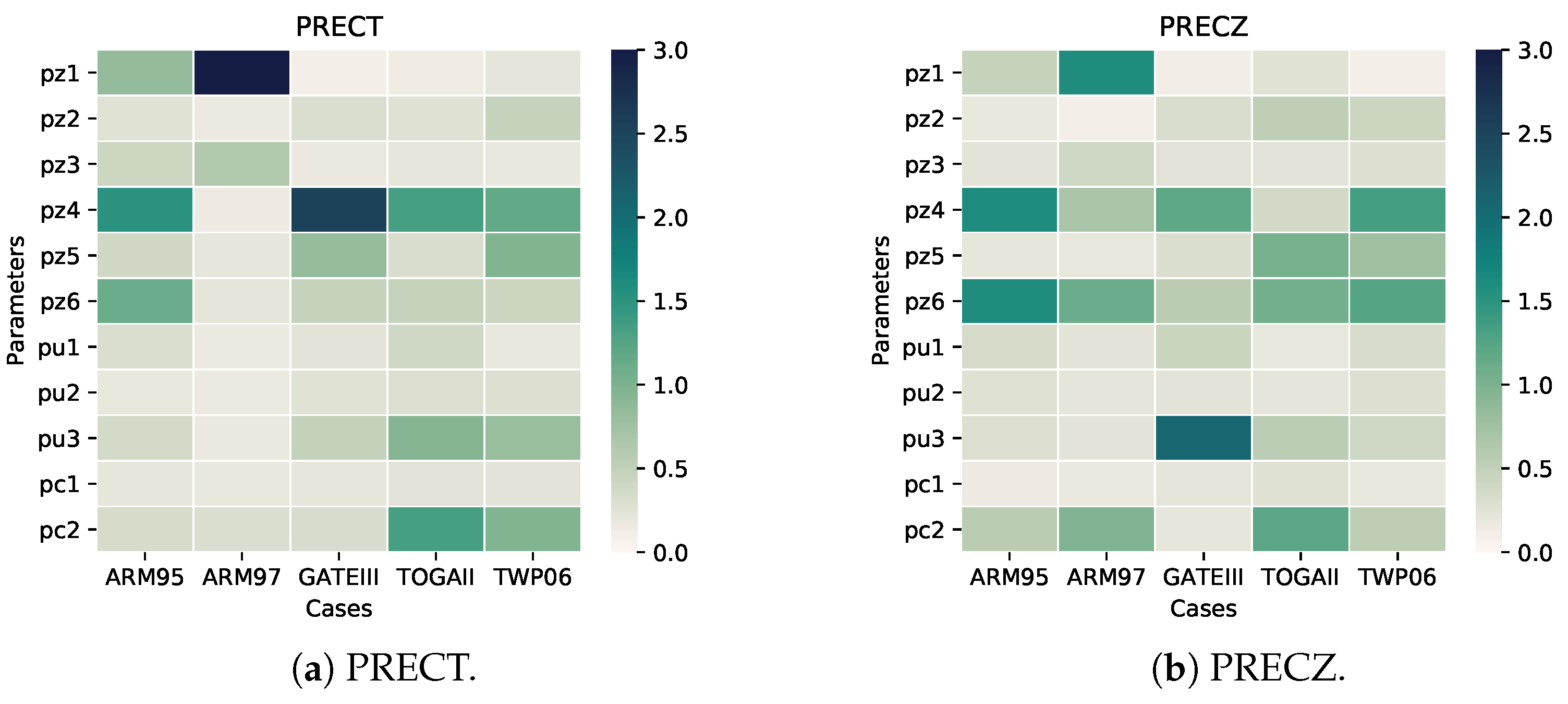
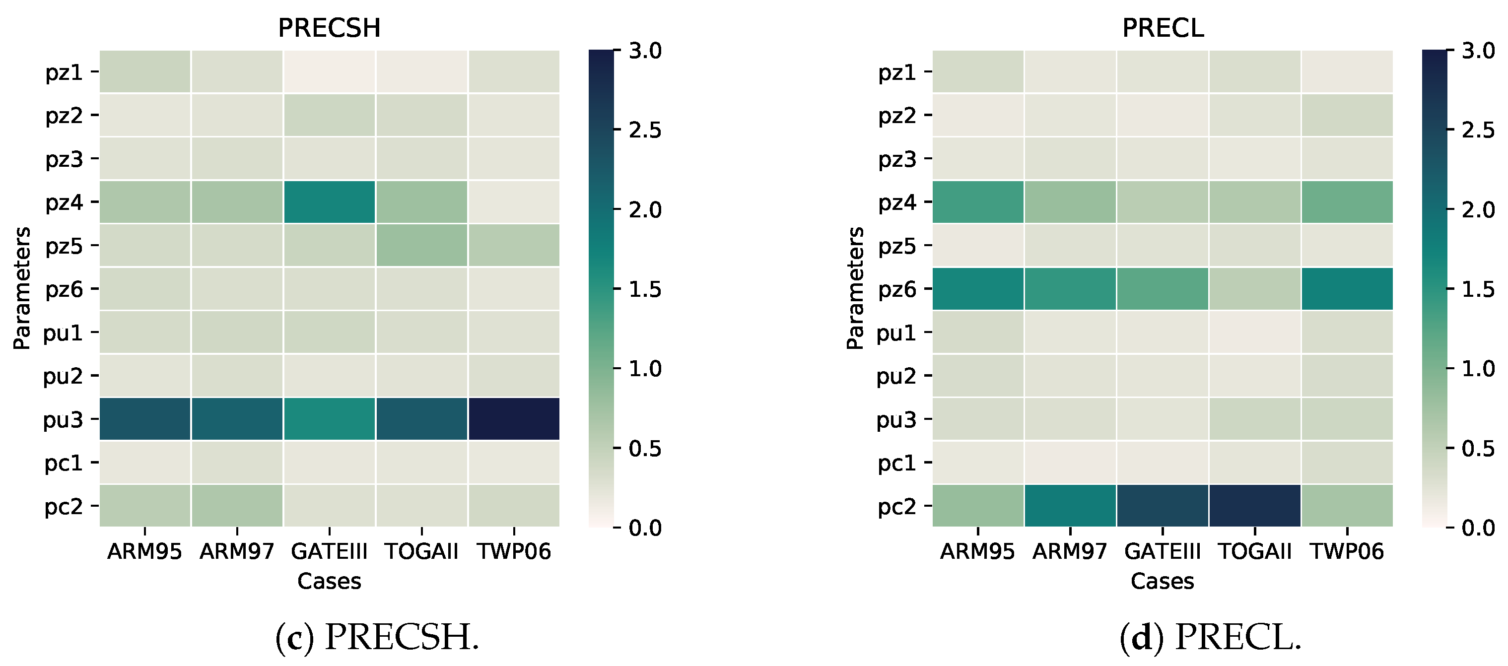
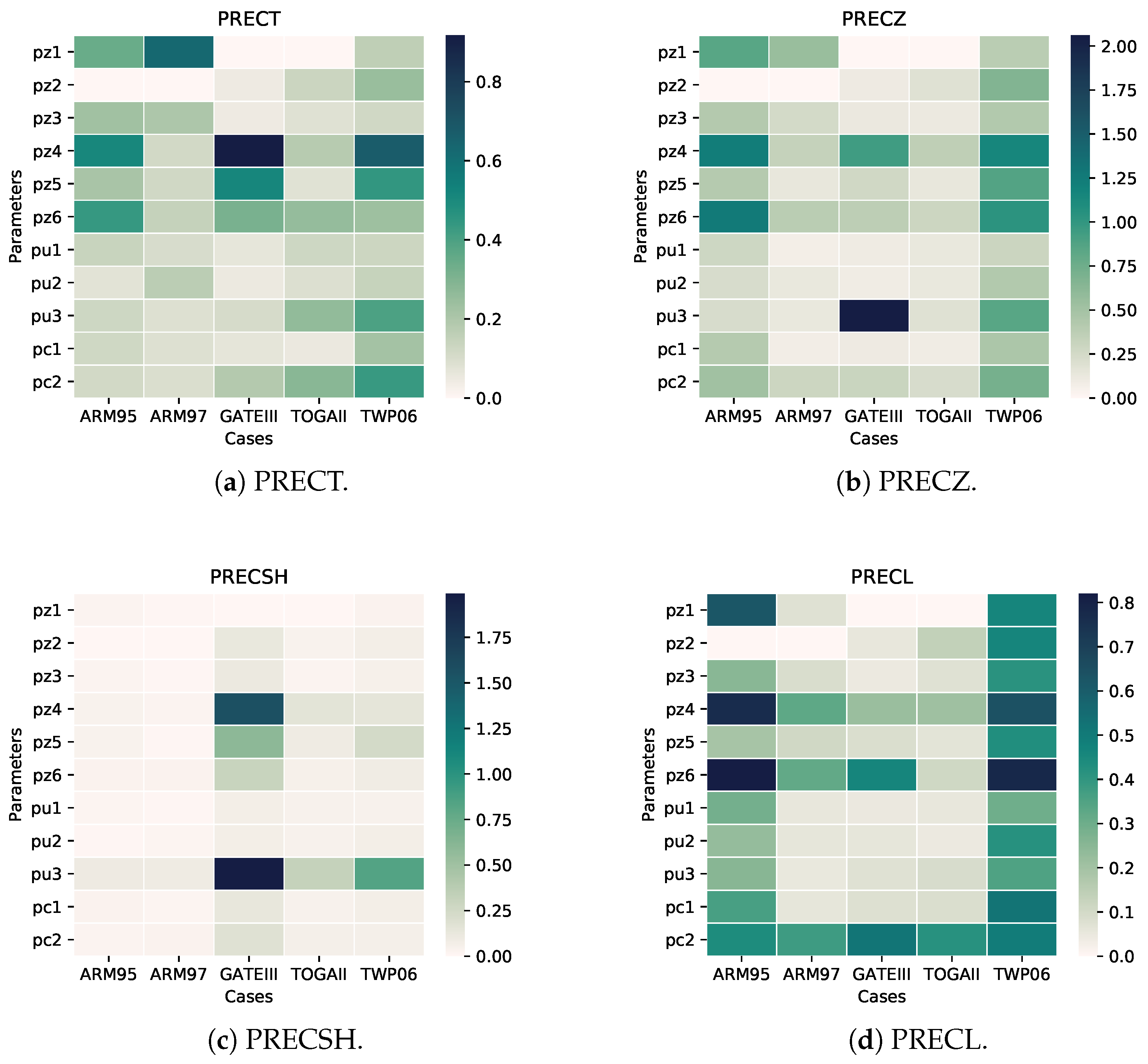
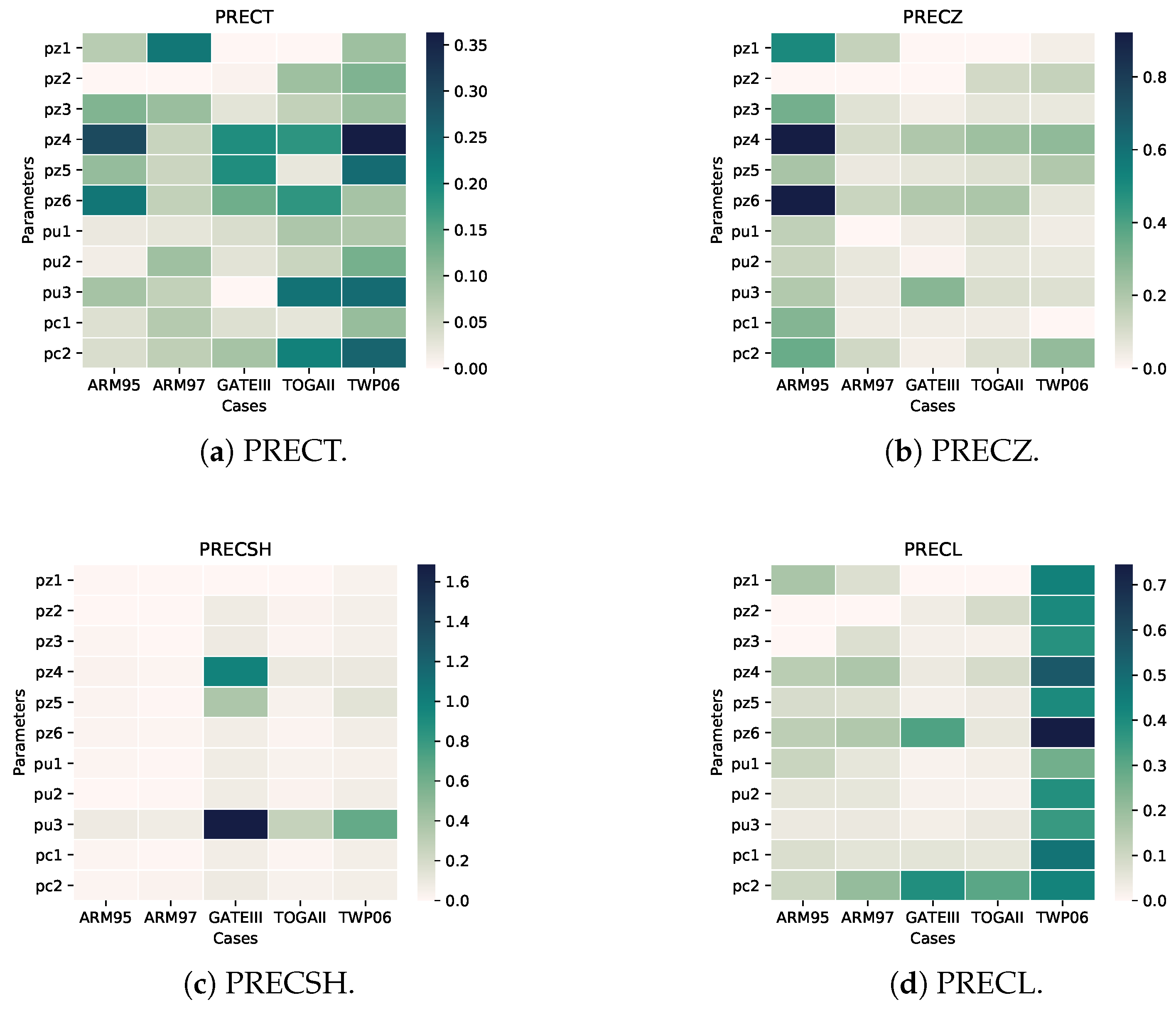
Heat maps allow the representation of 3D information in a 2D plane, increasing the readability of the picture. In these sets of plots, color is used to indicate the magnitude of the effect caused by the parameter change on the results. Among the five variables related to precipitation, their sensitivities represented by fusion are presented in Figure 2. Furthermore, in order to compare the differences between the relative and absolute biases of the different output variables, the magnitude of the change in the absolute value of the MABB representation is shown in Figure 3. Considering the non-linearity of the model and the variability of the cases, the positive and negative MABB values are also shown in Figure 4 and Figure 5, respectively. To facilitate reader comprehension, positive deviations and the absolute value of total deviations are represented in green, while negative deviations are shown in blue. The deeper the color, the greater the deviation. Positive and negative deviations are based on the default output, aiming to verify whether the magnitude of the impact on the results is the same when the parameter adjustment ranges are identical. In other words, this is to determine whether the impact is linear.
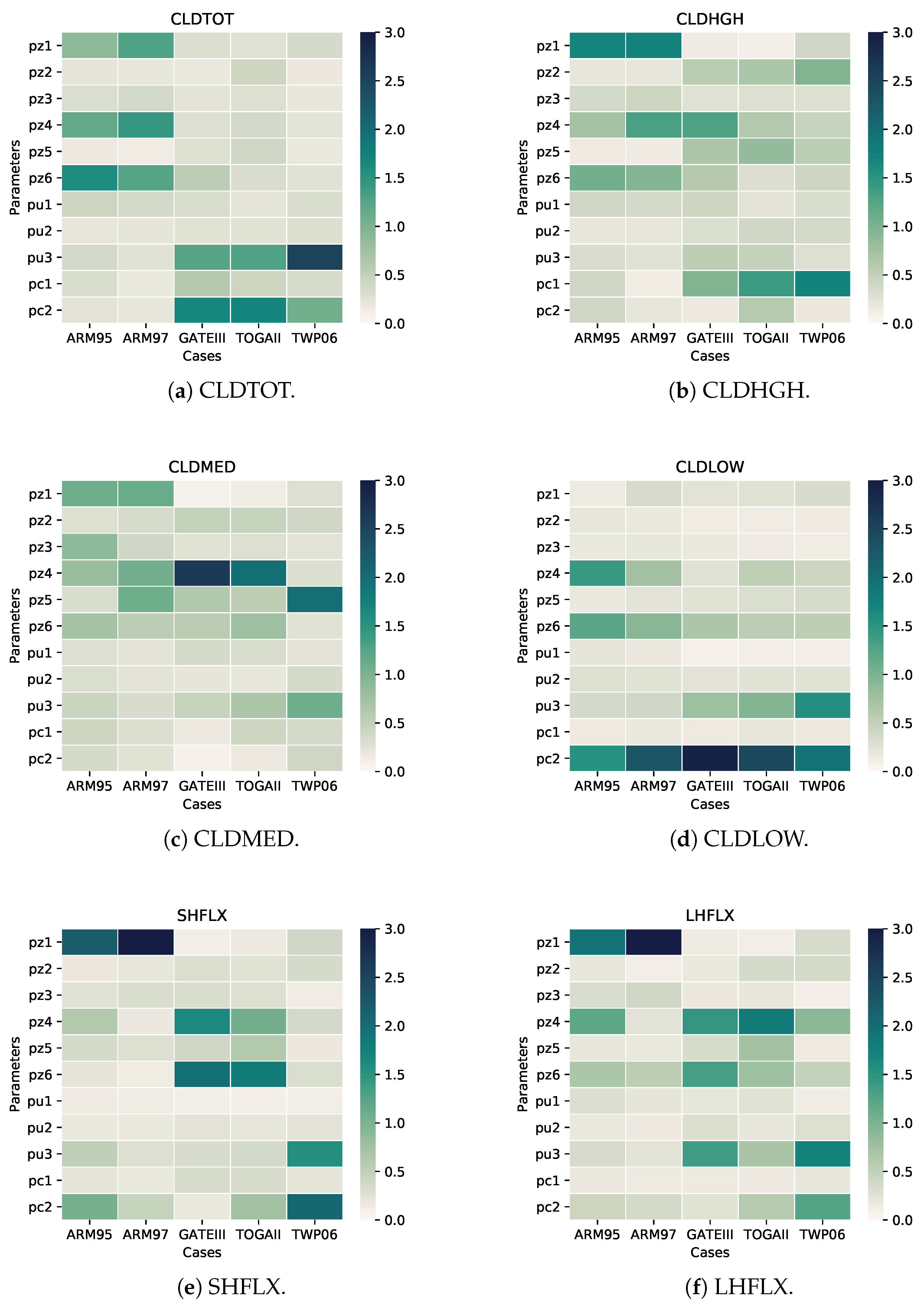
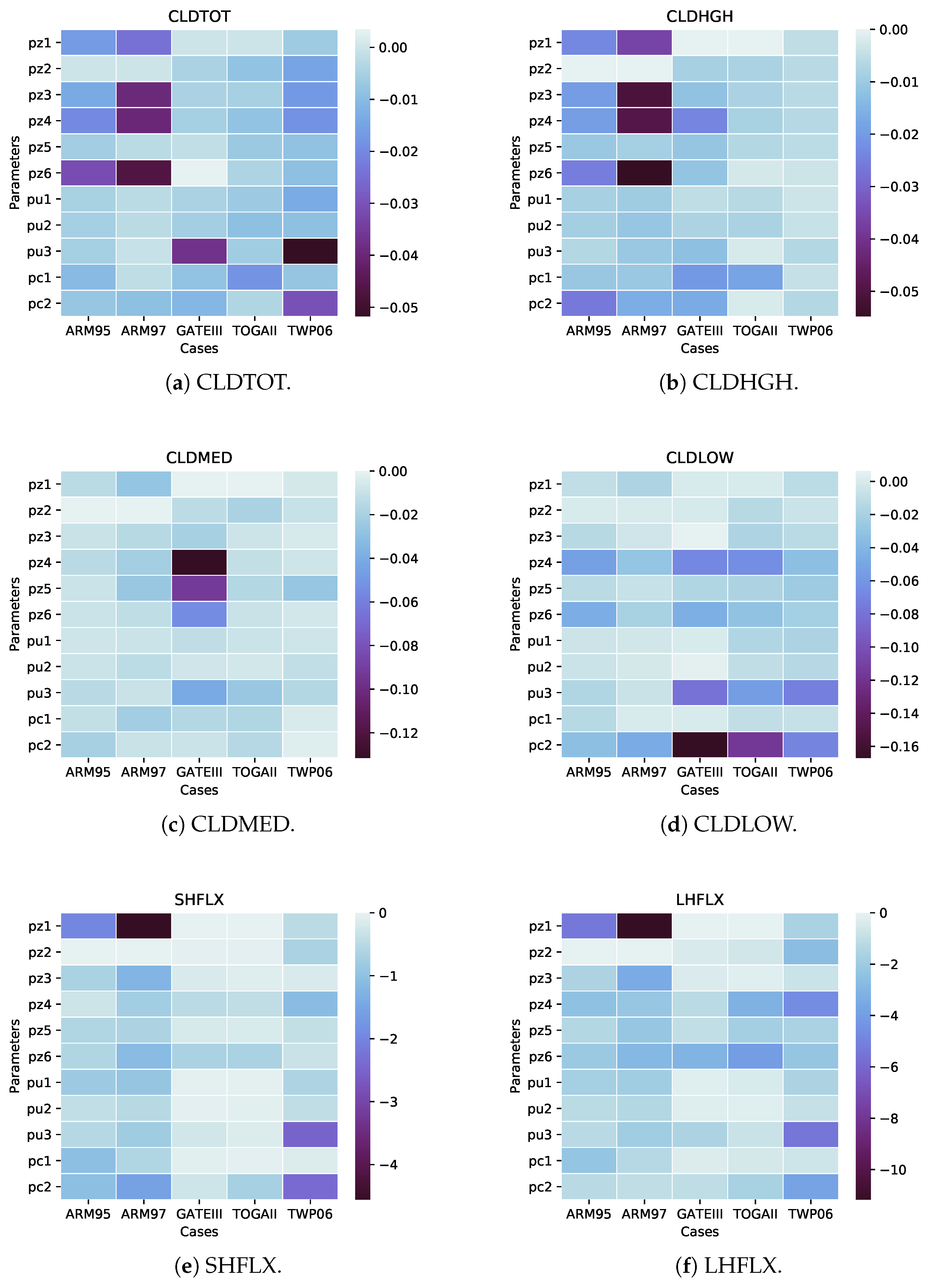
For clouds as well as heat fluxes, the results of the sensitivity analysis of their relevant output variables are shown in Figure 6. The meaning of these is the same as in Figure 2. Similarly, Figure 6 shows their MRBB, Figure 7 their MABB, while Figure 8 and Figure 9 show the MABB for the case of considering positive and negative variations, respectively.
With regard to an SCAM case, the impact of different parameters on the output variable is inconsistent and can vary significantly (by more than 10 times). Even for the same parameter, its effects in different cases are not consistent. For example, pz1 (c0_lnd) has very little effect when the observation point is located in the tropical ocean, while pz2 affects land. Parameter pu3 has a significant impact on shallow convective precipitation (PRECSH), with an influence hundreds of times greater than other parameters.
In the same parameter space, the range of changes in different output variables varies. For example, the range of change for PRECSH is notably large, likely due to its typically small values (usually only a few millimeters per day).
For CLDTOT and CLDHGH, the two land convection cases exhibit a greater range of change, particularly evident in c0_lnd, tau, and alfa. For CLDLOW, rhminl has a more significant impact on GATEIII and TOGAII. Additionally, rkm greatly influences the sensible heat flux of TWP06.
The results of the aforementioned experiments fully demonstrate the significant practical value of the proposed solution in this paper. These findings indicate that with the powerful computational capabilities of HPC, it is possible to conduct large-scale parameter testing in a relatively short period of time.

5. Discussion

Previous studies have often focused on global models (such as CAM) [47] or on a limited number of specific cases [48], typically examining the models themselves. In contrast, this paper emphasizes the overall methodology for parameter testing and aims to develop an integrated approach for large-scale parameter testing suitable for HPC environments. To verify the efficiency and effectiveness of this approach, we analyzed the different impacts of 11 parameters on 10 output variables using SCAM as an example in the previous section’s experiments. From the results, we can observe several interesting conclusions.
First, regarding precipitation output, although PRECT is the sum of various precipitation components, it is clear that the sensitivity of PRECT to different parameters is not a simple sum of the sensitivities of its individual components. There are both commonalities and individual characteristics across different cases. For example, the output of PRECSH shows high consistency across different cases, indicating two points. On the one hand, PRECSH is less affected by the specific characteristics of the cases, such as location and season. On the other hand, its absolute value is relatively small, thus contributing less to the total precipitation. The parameter pu3, or rkm, has a significant impact on the results, confirming the role of the UW scheme in shallow convective precipitation and the importance of rkm relative to other parameters. The heatmaps of PRECT and PRECZ are more similar, reflecting that deep convective precipitation remains the main component of total precipitation in the five cases studied. Additionally, for total precipitation and deep convective precipitation, the impact of pz4, or tau, is significant and should be a focus for future research. Conversely, pc2, or rhminl, has a major impact on large-scale precipitation, especially in GATEIII and TOGAII, both of which are fully oceanic cases.
For cloud-related variables, similar conclusions can be drawn. For all five cases studied, pc2, or rhminl, has a greater impact on CLDLOW, but not on the other three variables. Overall, ARM95/97 is more influenced by the ZM deep convection scheme, making these two cases exhibit different parameter sensitivities compared to the other three tropical convective cases. This phenomenon is also evident in the two heat flux variables, where pz1, or c0_lnd, overwhelmingly impacts the output, which is closely related to the fact that these two cases are located in land regions. Conversely, pz4 and pz6 have a greater impact on tropical ocean cases. Interestingly, TWP06 shows different sensitivities in SHFLX, which warrants further investigation.
When we separate the positive and negative impacts of MABB, we also find some interesting conclusions. For example, although we adjust each parameter in a symmetric space relative to the default value, their effects on precipitation are not uniform. This is particularly evident in PRECZ and PRECL. In ARM95, PRECZ is more likely to be positively influenced, while PRECL is more likely to be negatively influenced. However, for TWP06, the opposite is true. For cloud and heat flux variables, the differences between positive and negative impacts are not very significant. Although there are some quantitative differences, they do not affect the qualitative conclusions.
In summary, the method and framework proposed in this paper provide the possibility for large-scale parameter testing based on HPC, helping researchers quickly identify the most impactful parameters. This allows for more targeted and detailed studies of different parameters in various application scenarios. Of course, the method proposed in this paper is not perfect. The study has not yet delved into further optimization of the model itself, indicating room for future improvement.

6. Conclusions

High-performance computing (HPC) is critically important in scientific computing, providing the computational power required to tackle complex problems and perform large-scale simulations. In Earth numerical modeling, HPC enables detailed simulations of atmospheric, oceanic, and land processes, offering valuable insights into Earth system dynamics. The method proposed in this paper further extends the scope of HPC applications by optimizing parameter analysis and tuning processes. Experimental results show that leveraging HPC’s computational capabilities makes large-scale parameter analysis experiments feasible, thereby enhancing the performance of corresponding models in simulations.
From the experimental results of the test cases, it can be seen that the 11 parameters have varying degrees of impact on the 10 output variables in the five typical SCAM cases. Quantitatively, the difference in their impact can be more than tenfold, and even several dozen times in some instances. This clearly demonstrates that different parameters from various parameterization schemes play different roles depending on the location and time of the outputs. This insight will inspire further research into parameterization schemes, emphasizing the need to set different parameter values for different application scenarios to improve model performance. It also shows that single-column models are indeed powerful tools for studying parameterization schemes.
Climate change concerns the future of human development, and improvements in methodology are significant from scientific research to policy-making. This study shows that it is necessary to optimize different parameters for different outputs in various locations. Extending this idea, it becomes clear that policymakers in different countries and regions also need to adopt appropriate strategies tailored to their specific conditions. This collective effort will help maintain a healthy climate and ecological environment, achieving sustainable development of the natural environment for the benefit of all humanity.

Author Contributions

Conceptualization, J.G.; methodology, J.G.; software, J.G.; validation, J.G., J.H. and X.C.; formal analysis, X.C.; investigation, X.C.; resources, X.C.; data curation, J.H.; writing—original draft preparation, J.G.; writing—review and editing, X.C.; visualization, J.G.; supervision, L.H.; project administration, G.X.; funding acquisition, J.H. All authors have read and agreed to the published version of the manuscript.

Funding

This work was supported in part by Key Scientific and Technological R&D Plan of Jilin Province of China under Grant 20230201066GX, in part by the Talent Project of the Department of Science and Technology of Jilin Province, China, under Grant 20240602106RC, in part by the National Natural Science Foundation of China under Grant 62202119, in part by the National Key Research and Development Plan of China under Grant 2017YFA0604500 and 2020YFB0204800, in part by the China Postdoctoral Science Foundation under Grant 2023M731950, and in part by the Central University Basic Scientific Research Fund under Grant 2023-JCXK-04.

Data Availability Statement

The data presented in this study are available on request from the corresponding author. The data are not publicly available due to privacy.

Conflicts of Interest

The authors declare no conflicts of interest.

Abbreviations

The following abbreviations are used in this manuscript:
HPCHigh-Performance Computing
ESMEarth System Model
SCAMSingle Column Atmosphere Model
SASensitivity Analysis

References

  1. Li, Y.; Duan, X.; Gan, L.; Wan, W.; Chen, Y.; Xu, K.; Yang, J.; Liu, W.; Xue, W.; Fu, H.; et al. Enabling Large-Scale Simulation of CAM on the Sunway TaihuLight Supercomputer. IEEE Trans. Comput. 2022, 71, 824–837. [Google Scholar] [CrossRef]
  2. Gao, P.; Duan, X.; Schmidt, B.; Wan, W.; Guo, J.; Zhang, W.; Gan, L.; Fu, H.; Xue, W.; Liu, W.; et al. Redesign and Accelerate the AIREBO Bond-Order Potential on the New Sunway Supercomputer. IEEE Trans. Parallel Distrib. Syst. 2023, 34, 3117–3132. [Google Scholar] [CrossRef]
  3. Gao, P.; Duan, X.; Schmidt, B.; Zhang, W.; Gan, L.; Fu, H.; Xue, W.; Liu, W.; Yang, G. Optimization of Reactive Force Field Simulation: Refactor, Parallelization, and Vectorization for Interactions. IEEE Trans. Parallel Distrib. Syst. 2022, 33, 359–373. [Google Scholar] [CrossRef]
  4. Wan, W.; Gan, L.; Wang, W.; Yin, Z.; Tian, H.; Zhang, Z.; Wang, Y.; Hua, M.; Liu, X.; Xiang, S.; et al. 69.7-PFlops Extreme Scale Earthquake Simulation with Crossing Multi-faults and Topography on Sunway. In Proceedings of the International Conference for High Performance Computing, Networking, Storage and Analysis, SC 2023, Denver, CO, USA, 12–17 November 2023; Arnold, D., Badia, R.M., Mohror, K.M., Eds.; ACM: New York, NY, USA, 2023; pp. 10:1–10:15. [Google Scholar] [CrossRef]
  5. Chen, Y.; Liu, Y.; Shi, X.; Song, J.; Liu, X.; Gan, L.; Guo, C.; Fu, H.; Gao, J.; Chen, D.; et al. Lifetime-Based Optimization for Simulating Quantum Circuits on a New Sunway Supercomputer. In Proceedings of the 28th ACM SIGPLAN Annual Symposium on Principles and Practice of Parallel Programming, PPoPP 2023, Montreal, QC, Canada, 25 February–1 March 2023; Dehnavi, M.M., Kulkarni, M., Krishnamoorthy, S., Eds.; ACM: New York, NY, USA, 2023; pp. 148–159. [Google Scholar] [CrossRef]
  6. Juckes, M.; Taylor, K.E.; Durack, P.J.; Lawrence, B.; Sénési, S. The CMIP6 Data Request (DREQ, version 01.00.31). Geosci. Model Dev. 2020, 13, 201–224. [Google Scholar] [CrossRef]
  7. Balaji, V.; Taylor, K.E.; Juckes, M.; Lawrence, B.N.; Durack, P.J.; Lautenschlager, M.; Blanton, C.; Cinquini, L.; Denvil, S.; Elkington, M. Requirements for a global data infrastructure in support of CMIP6. Geosci. Model Dev. 2018, 11, 3659–3680. [Google Scholar] [CrossRef]
  8. Karpatne, A.; Atluri, G.; Faghmous, J.H.; Steinbach, M.; Banerjee, A.; Ganguly, A.; Shekhar, S.; Samatova, N.; Kumar, V. Theory-Guided Data Science: A New Paradigm for Scientific Discovery from Data. IEEE Trans. Knowl. Data Eng. 2017, 29, 2318–2331. [Google Scholar] [CrossRef]
  9. Vojacek, L.; Podhoranyi, M. Hpc Based Smart Remote Execution Solution for Modelling Environmental Issues. In Proceedings of the International Cognitive Cities Conference, Okinawa, Japan, 7–9 August 2018. [Google Scholar]
  10. Liu, L.; Yang, A.; Chen, L.; Xiong, W.; Jing, N. HiGIS—When GIS Meets HPC. In Proceedings of the 12th International Conference on GeoComputation, Wuhan, China, 23–25 May 2013. [Google Scholar]
  11. Guo, J.; Lai, Y.; Zhang, J.; Zheng, J.; Fu, H.; Gan, L.; Hu, L.; Xu, G.; Che, X. C3DA: A Universal Domain Adaptation Method for Scene Classification From Remote Sensing Imagery. IEEE Geosci. Remote Sens. Lett. 2024, 21, 6006705. [Google Scholar] [CrossRef]
  12. Liu, T. The Computer Information Technology Application of Big Data Era in Urban Planning and Design. In Cyber Security Intelligence and Analytics: Proceedings of the 2020 International Conference on Cyber Security Intelligence and Analytics (CSIA 2020); Springer: Berlin/Heidelberg, Germany, 2020. [Google Scholar]
  13. Guo, J.; Xu, Y.; Fu, H.; Xue, W.; Gan, L.; Tan, M.; Wu, T.; Shen, Y.; Wu, X.; Hu, L.; et al. GEO-WMS: An improved approach to geoscientific workflow management system on HPC. CCF Trans. High Perform. Comput. 2023, 5, 360–373. [Google Scholar] [CrossRef]
  14. Deelman, E.; Peterka, T.; Altintas, I.; Carothers, C.D.; Van Dam, K.K.; Moreland, K.; Parashar, M.; Ramakrishnan, L.; Taufer, M.; Vetter, J. The future of scientific workflows. Int. J. High Perform. Comput. Appl. 2018, 32, 159–175. [Google Scholar] [CrossRef]
  15. Tian, L.; Sedona, R.; Mozaffari, A.; Kreshpa, E.; Paris, C.; Riedel, M.; Schultz, M.G.; Cavallaro, G. End-to-End process orchestration of earth observation data workflows with apache airflow on high performance computing. In Proceedings of the IGARSS 2023–2023 IEEE International Geoscience and Remote Sensing Symposium, Pasadena, CA, USA, 16–21 July 2023; pp. 711–714. [Google Scholar] [CrossRef]
  16. Deelman, E.; Vahi, K.; Juve, G.; Rynge, M.; Callaghan, S.; Maechling, P.J.; Mayani, R.; Chen, W.; Da Silva, R.F.; Livny, M.; et al. Pegasus, a workflow management system for science automation. Future Gener. Comput. Syst. 2015, 46, 17–35. [Google Scholar] [CrossRef]
  17. Barseghian, D.; Altintas, I.; Jones, M.B.; Crawl, D.; Potter, N.; Gallagher, J.; Cornillon, P.; Schildhauer, M.; Borer, E.T.; Seabloom, E.W. Workflows and extensions to the Kepler scientific workflow system to support environmental sensor data access and analysis. Ecol. Inform. 2010, 5, 42–50. [Google Scholar] [CrossRef]
  18. Nan, D.; Wei, X.; Xu, J.; Haoyu, X.; Zhenya, S. CESMTuner: An Auto-tuning Framework for the Community Earth System Model. In Proceedings of the 2014 IEEE Intl Conf on High Performance Computing and Communications, 2014 IEEE 6th Intl Symp on Cyberspace Safety and Security, 2014 IEEE 11th Intl Conf on Embedded Software and Syst (HPCC, CSS, ICESS), Paris, France, 20–22 August 2014; pp. 282–289. [Google Scholar]
  19. Hazeleger, W.; Severijns, C.; Semmler, T.; Stefanescu, S.; Willen, U. EC-Earth: A Seamless Earth-System Prediction Approach in Action. Bull. Am. Meteorol. Soc. 2010, 91, 1357–1363. [Google Scholar] [CrossRef]
  20. Long, B.H.; Duong, P.X.; Minh-Thu, P. Using Regional Ocean Modeling System (ROMS) for hydrodynamic regime in Binh Cang-Nha Trang bay, Vietnam. J. Mar. Sci. 2019, 1, 1–6. [Google Scholar] [CrossRef]
  21. Booij, N.; Ris, R.C.; Holthuijsen, L.H. A third-generation wave model for coastal regions - 1. Model description and validation. J. Geophys. Res.-Oceans 1999, 104, 7649–7666. [Google Scholar]
  22. Ayik, A.; Ijumba, N.; Kabiri, C.; Goffin, P. Preliminary assessment of small hydropower potential using the Soil and Water Assessment Tool model: A case study of Central Equatoria State, South Sudan. Energy Rep. 2023, 9, 2229–2246. [Google Scholar] [CrossRef]
  23. Lindström, G.; Pers, C.; Rosberg, J.; Strömqvist, J.; Arheimer, B. Development and testing of the hype (Hydrological Predictions for the Environment) water quality model for different spatial scales. Hydrol. Res. Int. J. 2010, 41, 295–319. [Google Scholar] [CrossRef]
  24. Strebel, L.; Goergen, K.; Naz, B.; Bogena, H.; Vereecken, H.; Franssen, H.H. Modeling of a Forested Study Site with the Community Land Model Version 5 Using Climate Projections for the 21st Century; Copernicus Meetings: Barcelona, Spain, 2020. [Google Scholar]
  25. Jia-Wen, Z.; Fang, L.; Xiang, S. Preliminary Assessment of the Common Land Model Coupled with the IAP Dynamic Global Vegetation Model. Atmos. Ocean. Sci. Lett. 2014, 7, 505–509. [Google Scholar] [CrossRef]
  26. Hourdin, F.; Mauritsen, T.; Gettelman, A.; Golaz, J.C.; Balaji, V.; Duan, Q.; Folini, D.; Ji, D.; Klocke, D.; Qian, Y. The art and science of climate model tuning. Bull. Am. Meteorol. Soc. 2017, 98, 589–602. [Google Scholar] [CrossRef]
  27. Yang, B.; Wang, M.; Zhang, G.J.; Guo, Z.; Qian, Y.; Huang, A.; Zhang, Y. Simulated Precipitation Diurnal Variation With a Deep Convective Closure Subject to Shallow Convection in Community Atmosphere Model Version 5 Coupled With CLUBB. J. Adv. Model. Earth Syst. 2020, 12, 1–22. [Google Scholar] [CrossRef]
  28. He, F.; Posselt, D.J. The Sensitivity of Simulated Tropical Cyclones to Tunable Physical Parameters in Community Atmosphere Model. In AGU Fall Meeting Abstracts; NASA: Washington, DC, USA, 2014. [Google Scholar]
  29. Guo, J.; Zheng, J.; Xu, Y.; Fu, H.; Xue, W.; Wang, L.; Gan, L.; Gao, P.; Wan, W.; Wu, X.; et al. LB-SCAM: A learning-based method for efficient large-scale sensitivity analysis and tuning of the Single Column Atmosphere Model (SCAM). Geosci. Model Dev. 2024, 17, 3975–3992. [Google Scholar] [CrossRef]
  30. Houtekamer, P.L.; Mitchell, H.L. A Sequential Ensemble Kalman Filter for Atmospheric Data Assimilation. Mon. Weather Rev. 2001, 129, 123–137. [Google Scholar] [CrossRef]
  31. Zhang, H.; Tian, X. A Multigrid Nonlinear Least-squares Four-dimensional Variational Data Assimilation Scheme with Advanced Research WRF (ARW). J. Geophys. Res. Atmos. 2018, 123, 5116–5129. [Google Scholar] [CrossRef]
  32. Veronika, E.; Sandrine, B.; Meehl, G.A.; Senior, C.A.; Bjorn, S.; Stouffer, R.J.; Taylor, K.E. Overview of the Coupled Model Intercomparison Project Phase 6 (CMIP6) experimental design and organization. Geosci. Model Dev. 2016, 9, 1937–1958. [Google Scholar]
  33. Eichler, T.P. The impacts of a warming climate on winter mid-latitude cyclones in the NARCCAP model suite. Clim. Dyn. 2020, 54, 4379–4398. [Google Scholar] [CrossRef]
  34. Saltelli, A.; Aleksankina, K.; Becker, W.; Fennell, P.; Ferretti, F.; Holst, N.; Li, S.; Wu, Q. Why so many published sensitivity analyses are false: A systematic review of sensitivity analysis practices. Environ. Model. Softw. 2019, 114, 29–39. [Google Scholar] [CrossRef]
  35. Bogenschutz, P.A.; Gettelman, A.; Morrison, H.; Larson, V.E.; Schanen, D.P.; Meyer, N.R.; Craig, C. Unified parameterization of the planetary boundary layer and shallow convection with a higher-order turbulence closure in the Community Atmosphere Model: Single-column experiments. Geosci. Model Dev. 2012, 5, 1407–1423. [Google Scholar] [CrossRef]
  36. Saltelli, A.; Annoni, P.; Azzini, I.; Campolongo, F.; Tarantola, S. Variance based sensitivity analysis of model output. Design and estimator for the total sensitivity index. Comput. Phys. Commun. 2010, 181, 259–270. [Google Scholar] [CrossRef]
  37. Goffart, J.; Rabouille, M.; Mendes, N. Uncertainty and sensitivity analysis applied to hygrothermal simulation of a brick building in a hot and humid climate. J. Build. Perform. Simul. 2015, 10, 37–57. [Google Scholar] [CrossRef]
  38. Morris, M.D. Factorial sampling plans for preliminary computational experiments. Technometrics 1991, 33, 161–174. [Google Scholar] [CrossRef]
  39. Plischke, E.; Borgonovo, E.; Smith, C.L. Global sensitivity measures from given data. Eur. J. Oper. Res. 2013, 226, 536–550. [Google Scholar] [CrossRef]
  40. Pianosi, F.; Wagener, T. Distribution-based sensitivity analysis from a generic input-output sample. Environ. Model. Softw. 2018, 108, 197–207. [Google Scholar] [CrossRef]
  41. Li, G.; Rabitz, H.; Yelvington, P.E.; Oluwole, O.O.; Bacon, F.; Kolb, C.E.; Schoendorf, J. Global Sensitivity Analysis for Systems with Independent and/or Correlated Inputs. J. Phys. Chem. A 2010, 2, 7587–7589. [Google Scholar] [CrossRef] [PubMed]
  42. Fu, H.; Liao, J.; Yang, J.; Wang, L.; Song, Z.; Huang, X.; Yang, C.; Xue, W.; Liu, F.; Qiao, F.; et al. The Sunway TaihuLight supercomputer: System and applications. Sci. China Inf. Sci. 2016, 59, 072001. [Google Scholar] [CrossRef]
  43. Gao, P.; Duan, X.; Guo, J.; Wang, J.; Song, Z.; Cui, L.; Meng, X.; Liu, X.; Zhang, W.; Ma, M.; et al. LMFF: Efficient and scalable layered materials force field on heterogeneous many-core processors. In Proceedings of the International Conference for High Performance Computing, Networking, Storage and Analysis, SC 2021, St. Louis, MO, USA, 14–19 November 2021; de Supinski, B.R., Hall, M.W., Gamblin, T., Eds.; ACM: New York, NY, USA, 2021; p. 42. [Google Scholar] [CrossRef]
  44. Gao, P.; Duan, X.; Zhang, T.; Zhang, M.; Schmidt, B.; Zhang, X.; Sun, H.; Zhang, W.; Gan, L.; Xue, W.; et al. Millimeter-Scale and Billion-Atom Reactive Force Field Simulation on Sunway Taihulight. IEEE Trans. Parallel Distrib. Syst. 2020, 31, 2954–2967. [Google Scholar] [CrossRef]
  45. Herman, J.; Usher, W. SALib: An open-source Python library for Sensitivity Analysis. J. Open Source Softw. 2017, 2, 97. [Google Scholar] [CrossRef]
  46. Stančin, I.; Jović, A. An overview and comparison of free Python libraries for data mining and big data analysis. In Proceedings of the 2019 42nd International Convention on Information and Communication Technology, Electronics and Microelectronics (MIPRO), Opatija, Croatia, 20–24 May 2019; pp. 977–982. [Google Scholar] [CrossRef]
  47. Qian, Y.; Yan, H.; Hou, Z.; Johannesson, G.; Klein, S.; Lucas, D.; Neale, R.; Rasch, P.; Swiler, L.; Tannahill, J. Parametric sensitivity analysis of precipitation at global and local scales in the Community Atmosphere Model CAM5. J. Adv. Model. Earth Syst. 2015, 7, 382–411. [Google Scholar] [CrossRef]
  48. Bogenschutz, P.A.; Tang, S.; Caldwell, P.M.; Xie, S.; Lin, W.; Chen, Y.S. The E3SM version 1 single-column model. Geosci. Model Dev. 2020, 13, 4443–4458. [Google Scholar] [CrossRef]
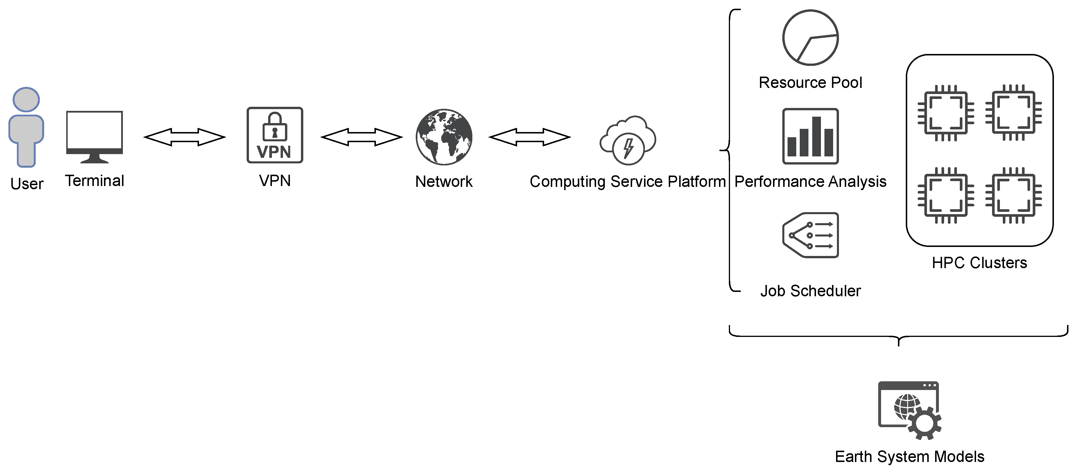
Figure 1. Diagram of the proposed framework structure.
Atmosphere 15 00935 g001
Figure 2. Fusion sensitivities of each parameter to precipitation variables.
Atmosphere 15 00935 g002aAtmosphere 15 00935 g002b
Figure 3. MABB of each parameter to each precipitation variable, when a single parameter is perturbed.
Atmosphere 15 00935 g003
Figure 4. Positive MABB of each parameter to each precipitation variable, when a single parameter is perturbed.
Atmosphere 15 00935 g004
Figure 5. Negative MABB of each parameter to each precipitation variable, when a single parameter is perturbed.
Atmosphere 15 00935 g005
Figure 6. Fusion sensitivities of each parameter to cloud variables, when a single parameter is perturbed.
Atmosphere 15 00935 g006
Figure 7. MABB of each parameter to cloud and heat flux variables, when a single parameter is perturbed.
Atmosphere 15 00935 g007
Figure 8. Positive MABB of each parameter to cloud and heat flux variables, when a single parameter is perturbed.
Atmosphere 15 00935 g008
Figure 9. Negative MABB of each parameter to cloud and heat flux variables, when a single parameter is perturbed.
Atmosphere 15 00935 g009
Table 1. The five typical SCAM cases studied in this paper.
CaseFull NameLatLonDateType
ARM95ARM Southern Great Plains36−97July 1995Land convection
ARM97ARM Southern Great Plains36−97June 1997Land convection
GATEIIIGATE Phase III9−24August 1974Tropical convection
TOGAIITropical W. Pacific Convection−12131December 1992Tropical convection
TWP06Tropical Ocean Global Atmosphere−2154January 2006Tropical convection
Table 2. Sensitivity analysis method integrated in the proposed framework.
Name of MethodAbbr.Reference
Morris sensitivity analysisMorrisMorris [38]
Delta moment-independent measureDeltaPlischke et al. [39]
Sobol’ sensitivity analysisSobolSaltelli et al. [36]
PAWN sensitivity analysisPAWNPianosi and Wagener [40]
High-dimensional model representationHDMRLi et al. [41]
Random balance designs Fourier amplitude sensitivity testRBD-FASTGoffart et al. [37]
Table 3. The 11 parameters involved in the exemplary study.
Abbr.NameDescriptionLow RangeDefaultHigh RangeCategory
pz1c0_lndDeep convection precipitation efficiency over land0.002950.00590.00885zmconv_
pz2c0_ocnDeep convection precipitation efficiency over ocean0.02250.0450.0675zmconv_
pz3dmpdzParcel fractional mass entrainment rate−0.002−0.001−0.0002zmconv_
pz4tauTime scale for consumption rate deep CAPE180036005400zmconv_
pz5capelmtThreshold value for CAPE3570105zmconv_
pz6alfaMaximum cloud downdraft mass flux fraction0.050.10.15zmconv_
pu1rpenPenetrative updraft entrainment efficiency2.55.07.5uwschu_
pu2kevpEvaporative efficiency1 × 10 6 2 × 10 6 3 × 10 6 uwschu_
pu3rkmUpdraft lateral mixing efficiency71421uwschu_
pc1rhminhThreshold relative humidity for stratiform high clouds0.70.80.9cldfrc_
pc2rhminlThreshold relative humidity for stratiform low clouds0.79750.89750.9975cldfrc_
Table 4. List of output variables used for sensitivity analysis.
NameDescriptionUnit
PRECTTotal precipitation ratem/s
PRECZDeep convective precipitation ratem/s
PRECSHShallow convective precipitation ratem/s
PRECLLarge-scale precipitation ratem/s
CLDTOTVertically-integrated total cloudPercentage
CLDLOWVertically-integrated low cloudPercentage
CLDMEDVertically-integrated mid-level cloudPercentage
CLDHGHVertically-integrated high cloudPercentage
SHFLXSurface sensible heat fluxW/m2
LHFLXSurface latent heat fluxW/m2
Disclaimer/Publisher’s Note: The statements, opinions and data contained in all publications are solely those of the individual author(s) and contributor(s) and not of MDPI and/or the editor(s). MDPI and/or the editor(s) disclaim responsibility for any injury to people or property resulting from any ideas, methods, instructions or products referred to in the content.