1. Introduction
Nowcasting commonly pertains to the prediction of weather conditions during the next 0–2 h, with a specific emphasis on small-scale weather patterns, particularly those associated with intense convective weather events. When compared to large-scale weather systems, meso- and micro-scale systems display abruptness, intricate and varied mechanisms, and brief durations, which makes predicting precipitation in the near future exceedingly intricate and demanding. Radar echoes, known for their precise and detailed information in terms of time and space, are frequently utilized as powerful instruments for nowcasting. Currently, two prevalent methods for predicting precipitation in real-time are numerical weather prediction and radar echo extrapolation. Among these methods, radar echo extrapolation has emerged as the major strategy due to its superior accuracy and reliability [
1].
Traditional radar echo extrapolation or remote sensing image extrapolation based on the semi-Lagrangian (RPM-SL) [
2] advection scheme, such as centroid tracking, tracking radar echoes by correlation (TREC), the optical flow (OF) method, etc., achieve probabilistic or deterministic precipitation forecasting by calculating the optical flow of radar or satellite echo motion fields and adding random perturbations to the motion fields. This method consumes less computational resources and operates quickly [
3], but it relies on the advection equation and struggles to adequately address the development and decay processes of precipitation clouds. As the extrapolation time increases, the accuracy of echo extrapolation rapidly decreases. Short-term precipitation forecasting is a typical temporal–spatial prediction problem. With the rapid development of AI technology, especially the breakthrough progress and application effects of deep learning (DL) in computer vision and time-series problem processing, deep learning methods can mine spatial and temporal variation features from a large amount of historical meteorological satellite and radar data [
4,
5], resulting in higher-precision and more suitable short-term forecasting models for local severe weather systems.
The approaches used for spatiotemporal predictive learning can be divided into two main groups: recurrent-based models and recurrent-free models. Recently, researchers have been using spatiotemporal predictive learning models more often to predict precipitation in the near future. Recurrent-based models commonly utilize a hybrid design that integrates convolutional neural networks and recurrent units. “recurrent units” usually refer to the recurrent units used in recurrent neural networks (RNNs) [
6]. This hybrid technique enables the models to independently acquire knowledge about spatial correlations and temporal evolution characteristics in the data. They are typical examples of recurrent-based models, which are widely and frequently applied in the field of spatiotemporal sequence prediction. ConvLSTM [
7] enhances conventional LSTM architectures by including convolutional neural networks to effectively process visual input. PredNet [
8] utilizes a deep recurrent convolutional neural network that incorporates both bottom-up (extracting features from raw data, gradually building higher-level scene representations) and top-down (using higher-level contextual information to influence and correct the interpretation of lower-level data) connections to consistently forecast upcoming video frames. PredRNN [
9] introduces a spatiotemporal LSTM unit that can extract and retain spatiotemporal representations to capture both spatial and temporal data simultaneously. PredRNN++ [
10] incorporates gradient highway units to mitigate the issue of gradient vanishing and a Casual-LSTM module to sequentially connect spatial and temporal memories. Highway layers can effectively propagate gradients in very deep feedforward networks. In PredRNN++, to prevent the rapid vanishing of long-term gradients, a highway approach is needed to learn frame skipping. Therefore, a new spatiotemporal recurrent structure, the gradient highway unit, is proposed. PredRNN-V2 [
11] enhances model performance by incorporating curriculum-learning techniques and memory decoupling loss. Utilize memory decoupling loss to enable the dual memory cells to “perform their respective duties” by separately focusing on long-term temporal dependency information from left to right and short-term spatiotemporal dynamic information transmitted vertically. Additionally, a new curriculum-learning strategy is proposed, which uses RSS for encoding and SS for decoding, allowing PredRNN to learn long-term dynamic information from the contextual framework. The MIM [
12] incorporates a sophisticated non-stationary learning mechanism within the structure of the LSTM module in order to effectively process intricate time series data. PhyDNet [
13] clearly distinguishes between the dynamics of partial differential equations (PDEs) and the unknown complementing information in recurring physical units. MAU [
14] introduces a motion-aware unit that specifically captures motion information.
Although recurrent-based models are effective at dealing with spatiotemporal data, they frequently suffer from significant computational complexity, resulting in prolonged training and inference procedures. In addition, they are susceptible to problems such as gradient vanishing or gradient explosion during training, which can impact the convergence and stability of the model. On the other hand, recurrent-free models utilize a hybrid structure consisting of either convolutional neural networks or convolutional neural networks combined with attention mechanisms. Currently, advancements in recurrent-free models mostly rely on enhancements to SimVP (simpler yet better video prediction). SimVP does not use advanced modules such as RNN, LSTM, and Transformer, nor does it introduce complex training strategies like adversarial training and sampling learning. All its modules are composed of CNNs. They are typical examples of recurrent-free models, which are widely and frequently applied in the field of spatiotemporal sequence prediction.
SimVP [
15] is an innovative piece of work that merges the Inception module with the UNet architecture to acquire knowledge about temporal changes. Its temporal module is specifically built to be capable of running in parallel. TAU [
16] substitutes the essential Inception-UNet with an attention module, allowing the temporal module to be parallelized and also record long-term temporal evolution. TAU and gSTA [
17] enhance the IncepU module by implementing a streamlined and highly efficient design that does not depend on InceptionNet or a Unix-like architecture. Recurrent-based models utilize recurrent modules to make predictions about the following frame by using autoregressive approaches, which are commonly referred to as recurrent models. On the other hand, recurrent-free models, make predictions for all future frames simultaneously, using all the available frames as input. The IncepU module in SimVP [
15] is composed of a framework similar to Unet, which utilizes multi-scale elements from an architecture like Inception. Nevertheless, gSTA and TAU enhance the IncepU module by implementing a streamlined and optimized architecture, eliminating the requirement for InceptionNet or a UNet-like architecture. OpenSTL [
18] introduces MetaFormers [
19] to enhance the temporal modeling of recurrent-free models, facilitating recurrent-free spatiotemporal prediction learning. In this design, OpenSTL utilizes MetaFormers as the temporal module, which converts the input channels from the original C to inter-frame channels T × C. The recurrent-free models are improved by expanding the recurrent-free architecture and utilizing the benefits of MetaFormers. OpenSTL incorporates ViT [
20], UniFormer [
21], HorNet [
22], and MogaNet [
23] into recurrent-free models using MetaFormers. These MetaFormers replace the intermediate temporal modules in the original recurrent-free design.
While deep learning-based nowcasting systems have shown promising outcomes, different algorithms have displayed distinct predicting abilities. However, it is important to note that the occurrence, development, and mobility of radar echoes are quite intricate. Hence, evaluating and assessing the predictive capabilities of machine deep learning algorithms is beneficial for choosing deep learning methods that are suitable for specific regions and constructing the most effective deep learning models.
This paper utilizes a radar echo extrapolation method that combines the attributes of convolutional neural networks [
24] and the self-attention mechanism [
25]. This method excels in extracting both temporal and spatial data. This method is appropriate for applying radar echo pictures that exhibit significant correlations in both temporal and spatial variations. The results indicate that the SimVP-GMA model exhibits higher accuracy in predicting the echo contours, with the forecast outcomes closely aligning with the actual values in terms of intensity.
2. Data and Processing Methods
This study utilizes C-band weather radar data and ground precipitation data collected from the Helan Mountain region between 2017 and 2020. We perform a thorough analysis of numerous advanced models using diverse assessment measures. We enhance the SimVP model, which demonstrates outstanding performance, to create our own model, SimVP-GMA. These experiments focus on short-term weather forecasting within a time frame of 0–1 h. This work enhances the existing precipitation forecasting by implementing nowcasting, focusing on three specific aspects: This study examines the practical use of state-of-the-art spatiotemporal predictive learning models in predicting radar echo in real-time in the Yinchuan region. We suggest a novel model that efficiently combines the SimVP architecture and the group-mix attention (GMA) [
26] module without using recurrent connections. This enables the temporal module to be parallelized while accurately recording long-term temporal progression. The suggested technique exhibits exceptional performance in the prediction of near-term precipitation. By integrating the SCConv module [
27] into the encoder section of SimVP, we successfully restrict the duplication of features, resulting in a decrease in the number of model parameters and FLOPs while simultaneously improving the capability of feature representation.
2.1. Data Source
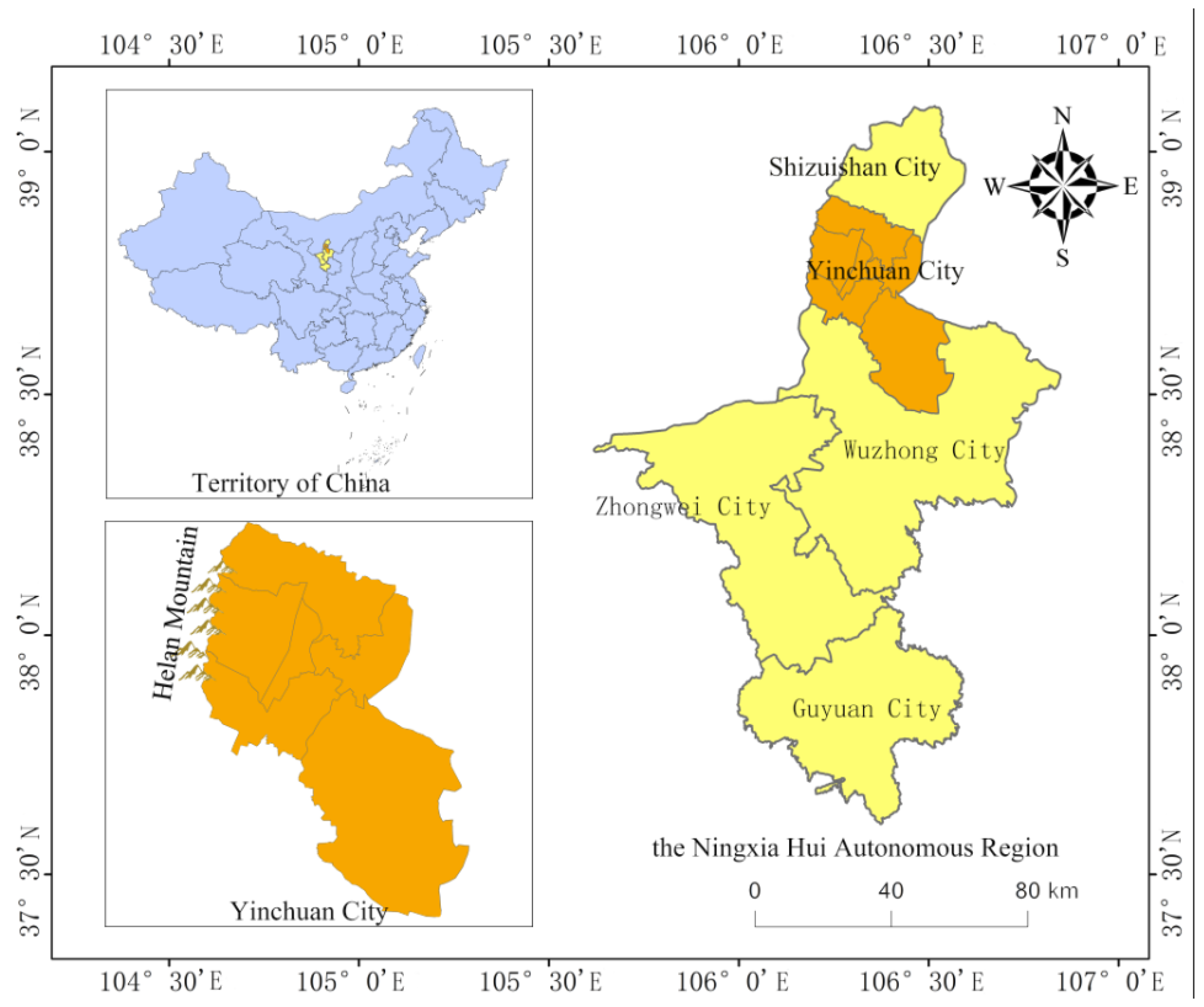
Yinchuan is located in the northwest of the Loess Plateau and the upper and middle reaches of the Yellow River. Its climate is semi-humid and semi-arid continental climate. This area is not only arid with little rainfall but has uneven spatial and temporal distribution of precipitation. Yinchuan straddles two climatic zones, namely, the summer warm Mediterranean climate (CSB) and the cool semi-arid climate (BSK). The main climatic features are scarce rain, snow, and strong water evaporation.
The research area is located on the east side of Helan Mountain, with geographical coordinates of 104° E–107° E and 37° N–40° N, and an altitude of 1000–3600 m. There is one C-band Doppler weather radar at Yinchuan station in the research area, with 254 surface rainfall stations. This radar has a wavelength of 1.5–3.75 cm, a frequency of 4000–8000 MHz, and adopts the VCP21 volume scan mode, which can complete scans at nine elevation angles within 5–6 min.The Drainage map of the study area is depicted in
Figure 1.
This study employs radar reflectivity factor (Z) data obtained during the rainy season (June to September) in Yinchuan City from 2017 to 2020. The mixed scanning data are acquired after performing encoding conversion, clutter suppression, attenuation correction, ground clutter correction, and coordinate transformation. The data have a resolution of 1 km × 1 km and are collected at 6-minute intervals. A dataset is constructed by selecting 28 precipitation processes with complete records as the research objects, based on data quality control and statistical analysis. Since most of the meteorological processes are relatively calm without precipitation, which is actually not conducive to learning the spatial and temporal information of precipitation on the network when selecting radar echo image data, in order to ensure the validity of the data, this part of the data without rain is eliminated. Finally, radar echo data with obvious precipitation processes are selected, including 28 precipitation processes with complete records.
We obtain precipitation fields from radar data, utilizing the Z/R relationship (the relationship between radar reflectivity factor and precipitation) and echo levels to determine the intensity and scope of precipitation fields. These 28 precipitation processes are related to the period from 2017 to 2020, representing different seasonal and typological precipitation events during this period. During the network training process, we have taken into account the diversity of seasons and precipitation types (including low-intensity, high-intensity, convective, stratiform, etc.), to ensure that the network can adapt to precipitation prediction tasks under various conditions. The continuous 2 h uninterrupted radar echo image data in the precipitation process is selected as a set of sample data, and the data are sliced. The models employed in this work utilize a sequence of ten consecutive radar echo images as input and generate predictions for the subsequent ten consecutive photos. These predictions aim to forecast the weather conditions for the upcoming 0 to 1 h.
2.2. Noise Reduction and Anomaly Handling
Radar echo intensities below 10 dBZ are mostly caused by clutter from ground dust, and this part of the data is considered noise for network learning. Therefore, it is necessary to set all pixel grid points below 10 dBZ in the image to 0. These relatively isolated interference echoes that exist in the dataset mostly appear in the form of isolated points or thin lines. The filtering method adopted in this paper involves establishing an N × N rectangular window on the radar echo data. If the number of valid pixels around the center point within the window area is less than a specified threshold, the center point is eliminated, meaning it is considered invalid data. The calculation formula is as follows:
N represents the window size, which is the total number of pixels within the rectangular region segmented on the image.
M represents the total number of valid pixels within the rectangular window.
is the percentage of valid reflectivity factors among all pixels in the rectangular window. When
is less than the given threshold, the pixel is considered an isolated data point and is eliminated.
2.3. Normalization Processing
For deep learning neural networks, to address issues such as gradient vanishing and gradient explosion that often arise in deeper network layers, and to improve computational efficiency, input data are typically normalized. Therefore, it is necessary to process radar echo data before model training, ensuring that the numerical range falls between 0 and 1. Firstly, the original radar reflectivity factor is linearly transformed into the pixel value range commonly used in image processing:
where “pixel” represents the transformed pixel value, falling within the range of 0 to 255. Secondly, normalization is applied. Here, we adopt the direct pixel normalization method commonly used in image processing, with the formula as follows:
Normalization allows the data to better fit within the gradient descent interval of the activation function, effectively mitigating the issue of gradient vanishing and accelerating the convergence speed of model training.
2.4. Data Augmentation
In the field of deep learning, a lack of training samples can easily lead to overfitting, where the model excessively fits the data in the training set, resulting in poor performance on the test set. The meteorological dataset constructed in this chapter still has a limited number of training samples for deep learning. Therefore, all experiments conducted in this paper subsequently employ data augmentation during the training phase. Data augmentation helps the neural network model learn more patterns and variations during the training process, enabling it to have stronger generalization capabilities in the face of uncertain changes in future data. During the model training process, data augmentation operations occur randomly at a certain proportion. Below are several methods used in this paper for data augmentation. (1) Random flip transformation: Horizontally or vertically flip the image sequence with a certain probability. (2) Random rotation transformation: Randomly rotate the selected image sequence by a certain angle. (3) Random reverse transformation: Reverse the selected image sequence with a certain probability.
3. SimVP-GMA
The purpose of this chapter is to examine the process of developing the SimVP-GMA model. Upon assessing the predictive accuracy of different deep learning algorithms, we noted that distinct models had diverse levels of performance across multiple measures. For example, although the SimVP model exhibited better performance based on the mean squared error (MSE) metric, it achieved a slightly lower score on the learned perceptual image patch similarity (LPIPS) metric. In order to tackle this issue, we suggest implementing the SimVP-GMA model, which combines the advantages of SimVP and the self-attention mechanism. This model demonstrates efficacy in capturing the interconnections between various points in the input sequence, hence enabling it to comprehend intricate dependencies within the sequence. The SimVP-GMA model demonstrated noteworthy performance in both the MSE and LPIPS criteria.
3.1. Model Introduction
Spatiotemporal predictive learning aims to infer future frames based on previous ones. Given a sequence
at time
t with the past
T frames, Our purpose is to predict the future sequence
at time
that contains the next
frames, where
is an image with the channel
C, height
H, and width
W.
. Formally, the predicting model is a mapping
with learnable parameters
, optimized by the following:
where
can be various loss functions, and we simply employ MSE loss in our setting.
The model framework suggested in this study is depicted in
Figure 2, as SimVP-GMA. More precisely, the spatial encoder is composed of two traditional 2D convolutional layers and a SCConv layer. On the other hand, the spatial decoder consists of a SCConv layer followed by two 2D transposed convolutional layers. We streamlined the initial four traditional convolutional layers into two standard 2D convolutional layers and a SCConv layer. This was conducted to minimize the computational expenses resulting from unnecessary feature extraction in visual tasks, while also promoting CNNs to produce more distinctive feature representations that encompass more comprehensive information. The GMA module stack, positioned between the spatial encoder and decoder, is tasked with extracting temporal data. Although our model has a relatively uncomplicated structure, it is proficient in acquiring spatial and temporal characteristics without depending on recurrent architectures.
During the encoding step, we utilize the encoder to sequentially incorporate
convolutional modules in order to extract spatial characteristics in a layered manner. Nevertheless, this method of stacking incurs a substantial expense in terms of computational resources, since conventional convolutional layers tend to extract a significant amount of duplicate features. In order to address this problem, we propose the implementation of the SCConv module (spatial and channel reconstruction convolution), which is designed to minimize unnecessary computations and enhance the acquisition of more meaningful features. SCConv is a plug-and-play architecture unit that may immediately substitute the usual convolutional layers in different convolutional neural networks. More precisely, the method for the encoding phase can be represented as follows, utilizing LayerNorm for downsampling:
represents the input data at time step i, where the input
and output
shapes are
and
. The Translator stage utilizes the GMA (group-mix attention) module, which acts as a sophisticated substitute for conventional self-attention. GMA can record relationships between individual tokens, between tokens and groups, and between multiple groups, regardless of their sizes. The SimVP-GMA model employs the use of GMA to arrange an encoder–decoder structure in the Translator. This arrangement aids in the extraction of temporal information and enables the achievement of temporal evolution effects. The formula is as stated:
where the input
and output
shapes are
and
The decoder phase employs 2
deconvolutions to recreate the ground truth frame by convolving C channels on (H, W), hence achieving the decoding of Translator information. The decoder transforms convolution operations into deconvolutions. The formula below illustrates the stacking technique employed by the decoder, which utilizes GroupNorm for upsampling:
where the shapes of input
and output
are
and
, respectively. We use ConvTranspose2d to serve as the unConv2d operator.
3.2. Spatial and Channel Reconstruction Convolution
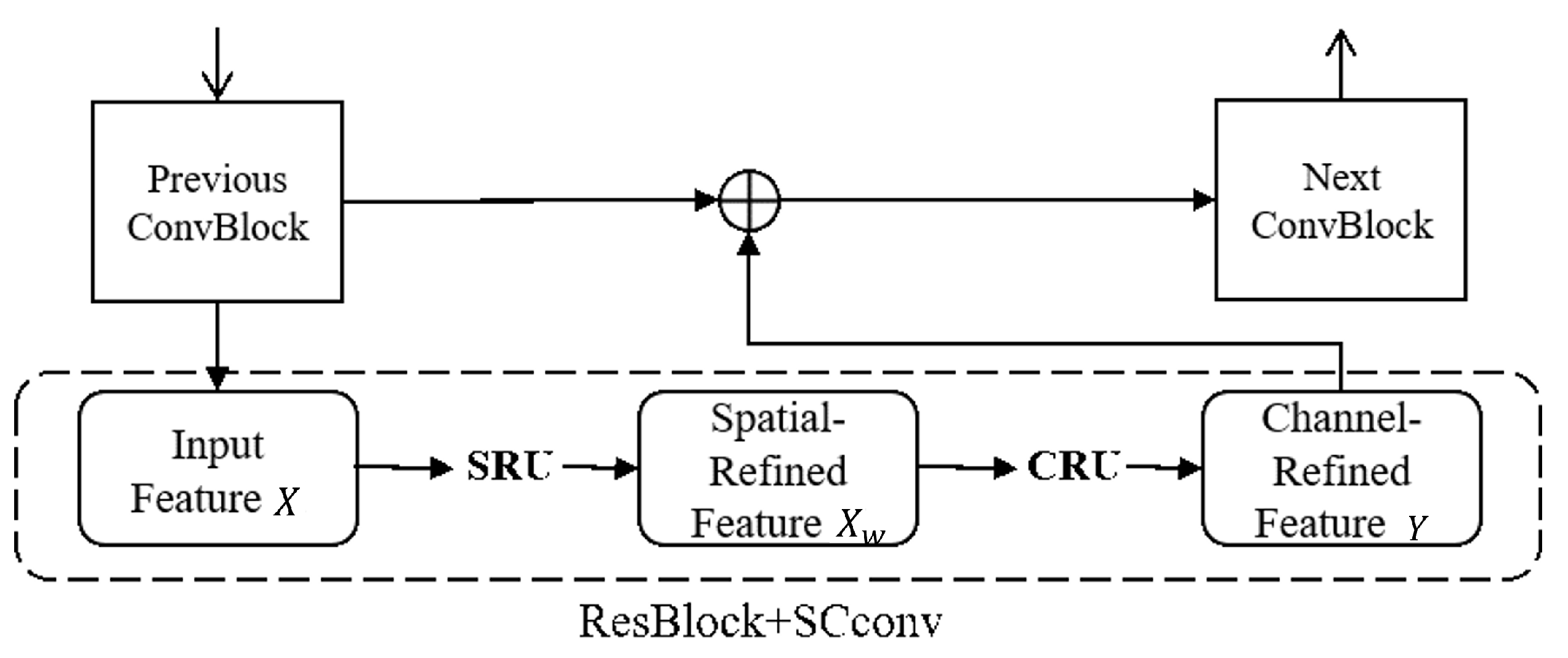
The encoder in the spatial module is composed of two traditional 2D convolutional layers and one SCConv layer. The SCConv module offers a novel approach to the feature extraction process of CNNs. It includes a strategy to optimize the utilization of spatial and channel redundancy information, with the goal of reducing redundant features and enhancing model performance. The SCConv module combines two essential components: the spatial reconstruction unit (SRU) and the channel reconstruction unit (CRU).
Figure 3 depicts the SCConv design, which integrates the SRU and CRU components. The figure accurately depicts the location of the SCConv module within the ResBlock.
The SCConv module consists of two units, namely SRU (spatial reconstruction unit) and CRU (channel reconstruction unit). SRU reduces spatial redundancy through a split reconstruction approach, while CRU employs a split–transform–merge method to minimize channel redundancy. These two units work together to reduce redundant information in CNN features. SCConv is a plug-in convolution module that can directly replace standard convolution operations and can be applied to various convolutional neural networks, thus reducing redundant features and computational complexity.
As shown in the diagram above, SCConv consists of two units: the spatial reconstruction unit (SRU) and the channel reconstruction unit (CRU), arranged in sequence. The input feature X first passes through the spatial reconstruction unit to obtain spatially refined feature . Then, it goes through the channel reconstruction unit to obtain the channel-refined feature Y as the output.
3.3. Group-Mix Attention
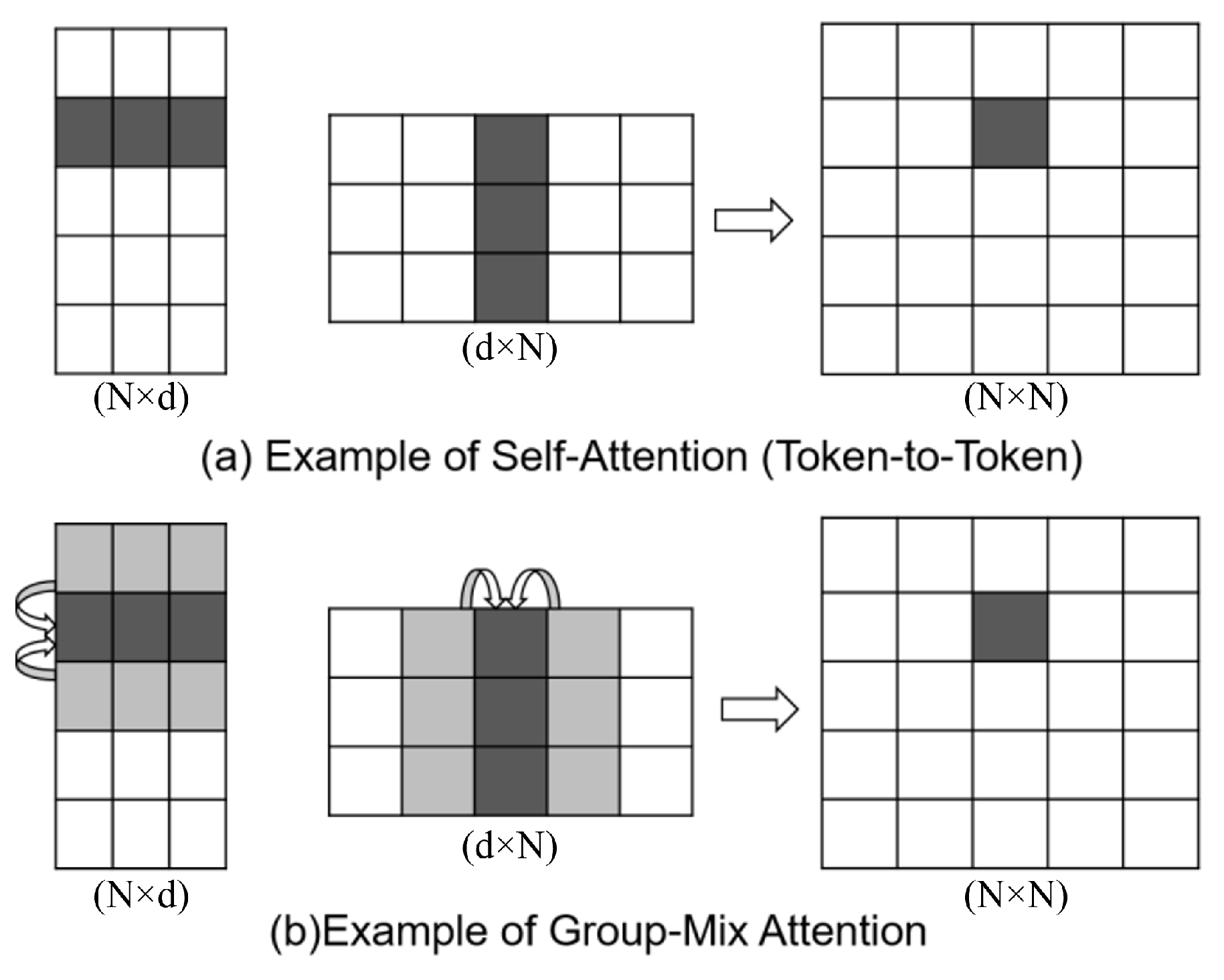
Visual transformers (ViTs) have demonstrated their ability to improve visual identification by including multi-head self-attention (MHSA), a technique that models long-range relationships. MHSA is commonly implemented as a query–key–value computation. Nevertheless, the attention maps produced from the query and key only record relationships between tokens at a singular level of detail. The GMA model utilizes a self-attention mechanism to effectively capture the relationships between individual tokens and groups of adjacent tokens. This allows for enhanced representational capabilities. Therefore, group-mix attention (GMA) can be considered a sophisticated substitute for conventional self-attention. It can capture correlations between tokens, between tokens and groups, and between groups themselves, all at varying group sizes.
Figure 4 depicts the precise calculation of GMA using five 3D tokens. In order to determine the correlation between two distinct groups, each consisting of three tokens, the groups are combined into two proxies, which will then be multiplied together. Group aggregation can be effectively accomplished using a sliding window-based operator, as depicted in the picture below.
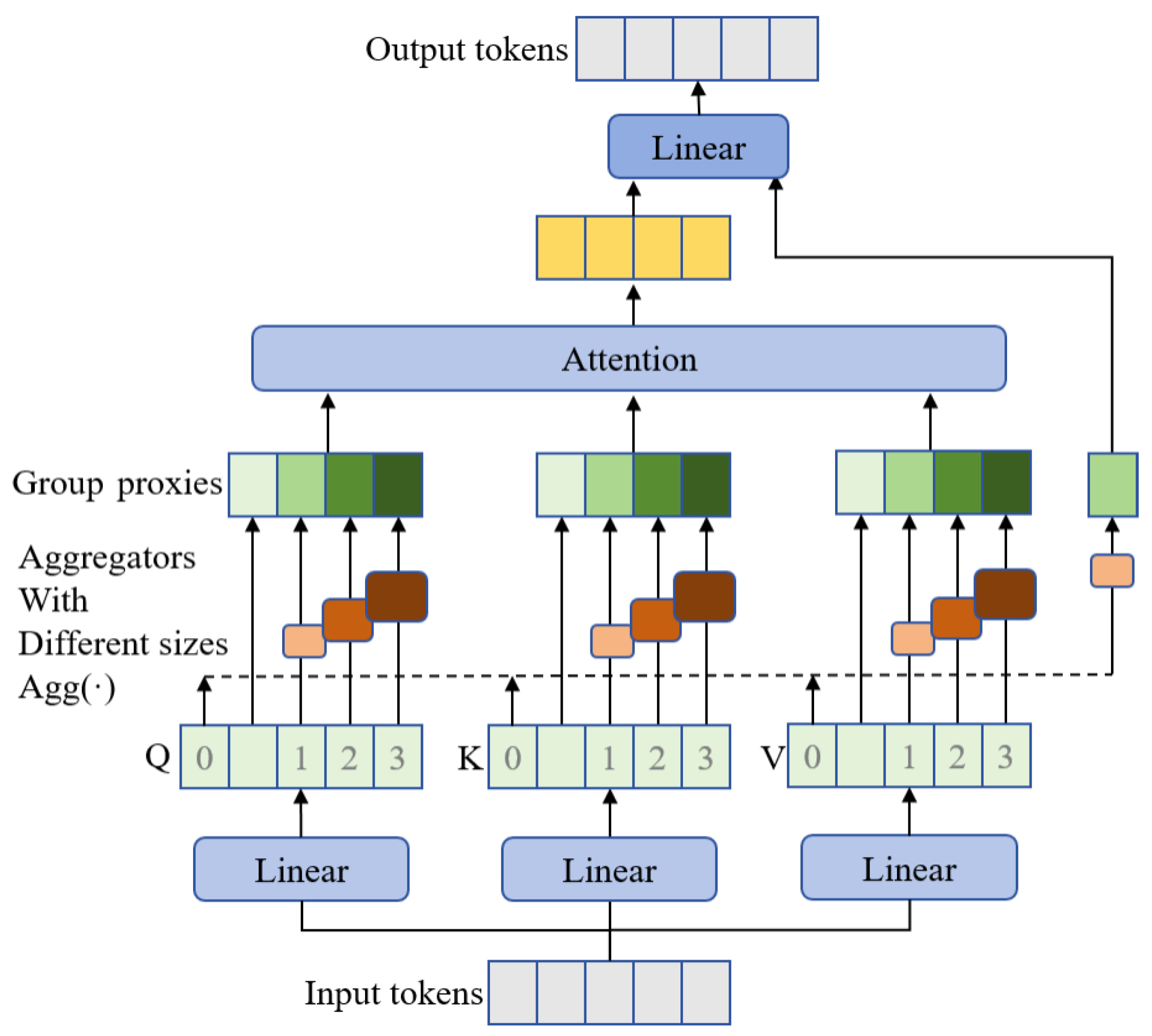
Within every GMA block, the components Q, K, and V are partitioned into five sections. To create group proxies, aggregators with varying kernel sizes are applied to four of these sections. This enables the computation of attention scores on combinations of individual tokens and group representatives at various levels of detail. The branch responsible for feeding the output into the attention computation is known as the pre-attention branch. The non-attention branch, located on the rightmost side, utilizes aggregation to establish several connections without attending to them. A linear mapping layer is used to combine the outputs of the attention branch with the non-attention branch. GMA divides query, key, and value into several pieces and applies various group aggregations to produce group proxies in a consistent manner. The attention map is computed by combining tokens and group proxies and is utilized to reassemble tokens and groups in Value.
Figure 5 depicts the structure of the group-mix attention block.
Following data preprocessing, the LayerNorm technique is initially utilized for downsampling. This is then followed by the application of SRU to decrease spatial redundancy and CRU to decrease channel redundancy. These two units cooperate to minimize repetitive data in CNN features. The Translator utilizes group-mix attention to extract temporal features, which enables temporal evolution effects. The output is then upsampled using GroupNorm to provide the projected outcomes.
5. Discussion
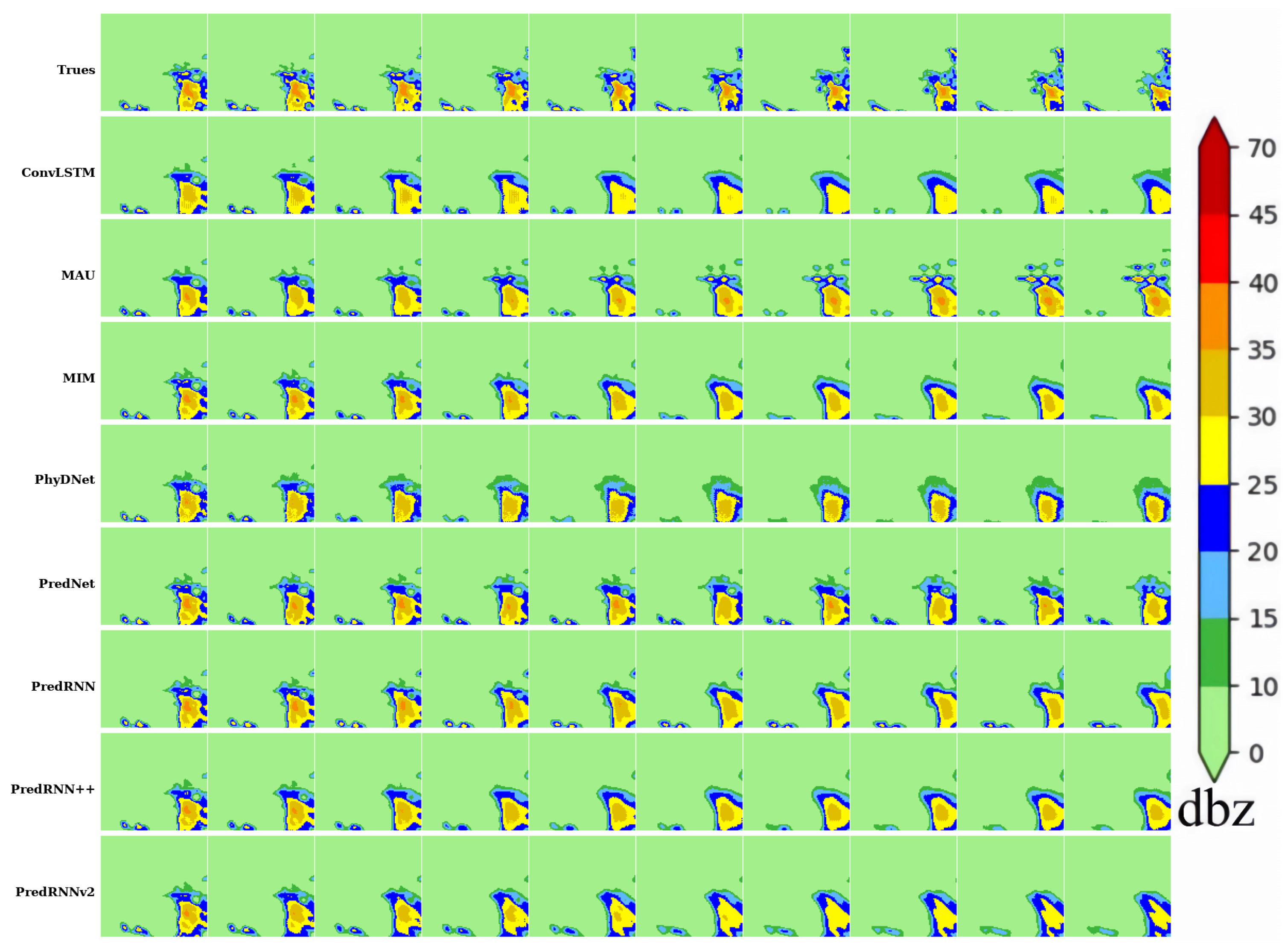
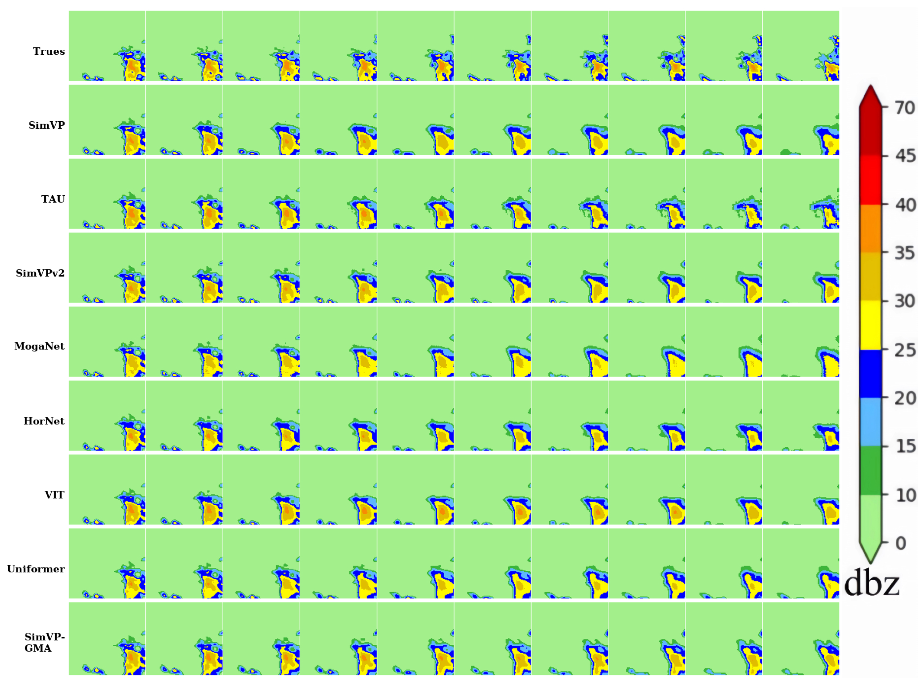
In order to make a meaningful comparison of the performance of each model, a sequence was selected at random from the test set, with a time interval of 6 min. The graphic was created by translating pixel data into radar echo values, assigning colors to each value range, and showing the results alongside the predictions of other models. The initial row of 10 images, captured at 6-minute intervals, represents the accurate output, while the subsequent rows display the prediction outcomes of each model for the same time periods.
Figure 6 presents the visualization results of the recurrent-based model; recurrent-based models often exhibit image-blurring as the forecasting time increases. The main reasons for this are as follows: Firstly, the loss of spatiotemporal information, which increases with longer forecasting periods; secondly, radar echo movement and evolution are influenced by factors such as wind speed and direction, temperature, and terrain. Using only radar echo images as model input cannot accurately predict changes in radar echoes, especially for the generation process of radar echoes from scratch. The forecasting effectiveness of the three convolutional recurrent neural network models based on a single data source is relatively weak. Thirdly, deep learning tends to average the error of the entire image during the training process, which causes the radar echo values to tend toward homogenization in the later stages of forecasting, resulting in visual “blurring”. Among them, PredRNN and PredRNN++ demonstrate good predictive capabilities for changes in echolocation and intensity and perform well among recurrent-based models. PredRNN++ has a certain forecasting ability for the echo center during longer forecast periods (1 h), but it underestimates the intensity. However, their forecasting ability for the echo generation process is relatively weak. The PredNet model, proposed for video prediction, performs exceptionally well on the evaluation metric of perceptual loss. However, due to its bottom-up mechanism, the predicted results produce repeated phenomena, where important features of the previous image are repeated every 12 min, making it difficult to accurately predict changes in echolocation.
Figure 7 presents the visualization results of the recurrent-free model. The performance of the recurrent-free model is basically better than that of the recurrent-based model, among which, our model SimVP-GMA performs excellently. Our SimVP-GMA model excels in producing smooth prediction results, particularly within the initial 24 min, where its performance surpasses that of other models. The addition of the GMA module, which captures long-term temporal evolution, results in a noticeable enhancement in the anticipated details as compared to SimVP. To summarize, the SimVP-GMA model exhibits outstanding performance when used for radar echo extrapolation through the utilization of deep learning techniques.
The SimVP-GMA model excels in various metrics, including mean squared error (MSE), mean absolute error (MAE), probability of detection (POD), critical success index (CSI), and a false alarm rate (FAR), collectively emphasizing its high accuracy in predicting the spatiotemporal evolution of radar echoes.
Two pivotal modules integrated into the SimVP-GMA model significantly contribute to its enhanced performance. These modules effectively capture long-term spatiotemporal dependencies, resulting in more precise and detailed prediction outcomes. Notably, the model is capable of generating smooth predictions within the initial 24 min, marking a notable advantage over other models. This characteristic is particularly valuable for applications requiring short-term radar echo extrapolation, such as weather forecasting and disaster management. Furthermore, the SimVP-GMA demonstrates robust predictive capabilities for both echo position and intensity variations up to 60 min, indicating its strength in handling radar echoes with high intensities and rapid changes.
Despite its remarkable performance, the SimVP-GMA model also faces limitations. The addition of modules leads to an increase in the number of model parameters and computational resources required, posing challenges during model deployment. Additionally, when predicting radar echoes with dBZ values exceeding 30, the model’s performance slightly diminishes, with a slightly lower CSI compared to the SimVP model. In conclusion, the SimVP-GMA model proposed in this study represents a significant improvement over existing models for radar echo extrapolation tasks. Future research will focus on reducing the number of parameters and computational complexity of the SimVP-GMA model while maintaining its performance and integrating multi-source data (such as wind speed, wind direction, temperature, and terrain information) for more accurate predictions.
