Deep-Learning Correction Methods for Weather Research and Forecasting (WRF) Model Precipitation Forecasting: A Case Study over Zhengzhou, China

Abstract

Systematic biases and coarse resolutions are major limitations of current precipitation datasets. Many studies have been conducted for precipitation bias correction and downscaling. However, it is still challenging for the current approaches to handle the complex features of hourly precipitation, resulting in the incapability of reproducing small-scale features, such as extreme events. In this study, we proposed a deep-learning model called PBT (Population-Based Training)-GRU (Gate Recurrent Unit) based on numerical model NWP gridded forecast data and observation data and employed machine-learning (ML) methods, such as Random Forest (RF), Support Vector Machine (SVM), K-Nearest Neighbor (KNN), and Gradient-Boosted Decision Tree (GBDT), to correct the WRF hourly precipitation forecasts. To select the evaluation method, we conducted a sample balance experiment and found that when the proportion of positive and negative samples was 1:1, the Threat Score (TS) and accuracy scores were the highest, while the Probability of Detection (POD) score was slightly lower. The results showed that: (1) the overall errors of the PBT-GRU model were relatively smaller, and its root mean square error (RMSE) was only 1.12 mm, which was reduced by 63.04%, 51.72%, 58.36%, 37.43%, and 26.32% compared to the RMSE of WRF, SVM, KNN, GBDT, and RF, respectively; and (2) according to the Taylor diagram, the standard deviation (${\mathsf{\sigma }}_{\mathrm{n}}$) and correlation coefficient (r) of PBT-GRU were 1.02 and 0.99, respectively, while the ${\mathsf{\sigma }}_{\mathrm{n}}$ and r of RF were 1.12 and 0.98, respectively. Furthermore, the ${\mathsf{\sigma }}_{\mathrm{n}}$ and r of the SVM, GBDT, and KNN models were between those of the above models, with values of 1.24 and 0.95, 1.15 and 0.97, and 1.26 and 0.93, respectively. Based on a comprehensive analysis of the TS, accuracy, RMSE, r and ${\mathsf{\sigma }}_{\mathrm{n}}$, the PBT-GRU model performed the best, with a significantly better correction effect than that of the ML methods, resulting in an overall performance ranking of PBT-GRU > RF > GBDT > SVM > KNN. This study provides a hint of the possibility that the proposed PBT-GRU model can outperform model precipitation correction based on a small sample of one-station data. Thus, due to its promising performance and excellent robustness, we recommend adopting the proposed PBT-GRU model for precipitation correction in business applications.

1. Introduction

With the continuous progress of mesoscale regional numerical models, numerical weather prediction (NWP) models have gained significant prominence in the domain of weather forecasting. However, the utilization of NWP models to forecast at finer temporal and spatial scales is currently constrained by several factors, including the initial conditions, boundary conditions, physical parametric schemes, and the integration of multi-source data fusion technology. To enhance the performance of NWP models, research on correction methods based on NWP models cannot be overlooked. A bias correction method serves as a bridge by connecting the NWP models with the realization of higher-resolution predictions. By correcting biases, the models become a more reliable tool for generating accurate predictions and supporting decision-making processes.

Significant advancements have been achieved in the field of correction method research. Hamill et al. [1] employed the technique of quantile mapping to align the precipitation frequency, resulting in enhanced forecast reliability, forecasting skills, and a reduction in the deterministic forecast bias. This approach also ensured the preservation of the precipitation distribution’s resolution and spatial details. Wu et al. [2] observed that the application of classical statistical methods led to a notable enhancement of the forecast results. The frequency-matching method and scoring optimization correction method, as proposed by Wu et al. [3], have gained significant popularity for the correction of cumulative precipitation forecasts. In recent years, the emergence of artificial intelligence has led to the successful utilization of machine-learning (ML) algorithms in various domains, such as data mining, image recognition, and medical care. These advancements have brought about significant transformations and disruptions in several industries. These advancements also serve as a point of reference and a source of inspiration for the advancement of weather-forecasting technology. For instance, Zaytar et al. [4] employed a multi-stacked Long Short-Term Memory (LSTM) approach to effectively model time series data of equal length. This methodology facilitated improved predictions of various meteorological variables, such as the wind speed, in nine different cities located in Morocco. Herman et al. [5] conducted a study in which they utilized three distinct statistical algorithms to forecast local extreme precipitation in the contiguous United States (CONUS). In their research, they employed a Random Forest (RF) training model for the purpose of precipitation prediction. Ahmed et al. [6] employed a range of ML algorithms, such as artificial neural networks (ANNs), K-Nearest Neighbor (KNN), and Support Vector Machine (SVM), to conduct a comparative analysis with the simulated precipitation and temperature outcomes generated by the general circulation models (GCMs). The study revealed that the K-Nearest Neighbor and related vector machine multi-model ensemble exhibited superior skills, whereas the ANNs demonstrated greater performance fluctuations across spatial domains. Xu [7] highlighted the increasing utilization of DL algorithms in weather forecasting and research in recent years. This has further emphasized their significant potential value and promising application prospects. Sun et al. [8] made a significant discovery regarding the application of DL algorithms in improving the accuracy of 10 m wind speed forecast results generated by numerical models. Their findings revealed that over time, the performance of the corrected forecasts exhibited a consistent improvement, with the effect becoming increasingly optimal. Shi et al. [9] utilized the convolutional Long Short-Term Memory (LSTM) model to forecast precipitation and observed that it exhibited superior performance compared to conventional optical flow extrapolation techniques. Guo et al. [10] discovered that DL algorithms have the capability to acquire the spatiotemporal structure and intrinsic correlation of radar data. This ability leads to a significant enhancement in the prediction accuracy of strong convective weather echo intensity. Teng [11] introduced a novel model known as RET-RNN, which was developed using LSTM and demonstrated promising results in the field of long-duration extrapolation.

However, unlike the consistent, continuous, and smooth temperature evolution, precipitation generally demonstrates a highly non-linear and random distribution in both space and time. Correcting precipitation data for bias is a challenge due to its complex characteristics. Various methods have been developed to address this issue, including traditional quantile mapping (QM)-based bias correction and downscaling techniques, as well as recent machine-learning-based approaches like Random Forest [12,13,14,15,16] and artificial neural networks [17]. In recent years, DL has made significant advancements across various fields and outperformed traditional ML methods due to its powerful ability to learn spatiotemporal feature representation in an end-to-end manner [18,19,20]. Specifically, DL approaches utilizing convolutional neural networks (CNNs) have been applied to correct and downscale low-spatial-resolution data [21,22,23], reanalysis products [24,25], and weather forecast model outputs [26,27]. While these studies have shown many promising strengths and advantages compared to traditional downscaling and correction methods, most of them struggle to capture local small-scale features, such as extreme events, in unseen datasets. For instance, Baño-Medina et al. [24] designed different DL configurations with varying numbers of plain CNN layers to correct and downscale daily ERA5-Interim reanalysis data from a spatial resolution of 2° to 0.5°. However, the overall performance still fell short when compared to simple generalized linear regression models, resulting in significant underestimation of precipitation extremes. Harris et al. [26] developed a generative adversarial network (GAN) architecture to correct and downscale weather forecast outputs and discovered that accounting for forecast errors (or biases) in a spatially coherent manner is more challenging than addressing pure downscaling problems. Additionally, previous studies on bias correction and downscaling have primarily focused on the daily time scale [24,25,26,27,28,29,30]. It is worth noting that understanding the distribution of hourly precipitation data within a day is more crucial than daily or monthly aggregations when assessing the impacts and risks associated with precipitation changes induced by global warming [31].

In this study, a combined model—PBT-GRU—based on the PBT (Population-Based Training) optimization algorithm and the GRU (Gate Recurrent Unit) model is constructed and trained, and a study on the correction method of the mesoscale numerical weather prediction (NWP) model’s WRF precipitation forecast is carried out by using the model. The objective of the proposed model is to offer significant guidance and technical assistance in enhancing the precision of refined precipitation forecasting and expanding its applicability in various business domains.

2. Data and Methodology

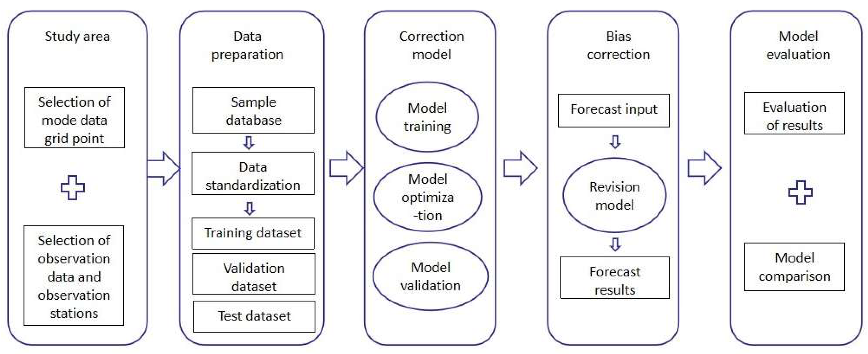
2.1. Scheme of Precipitation Correction

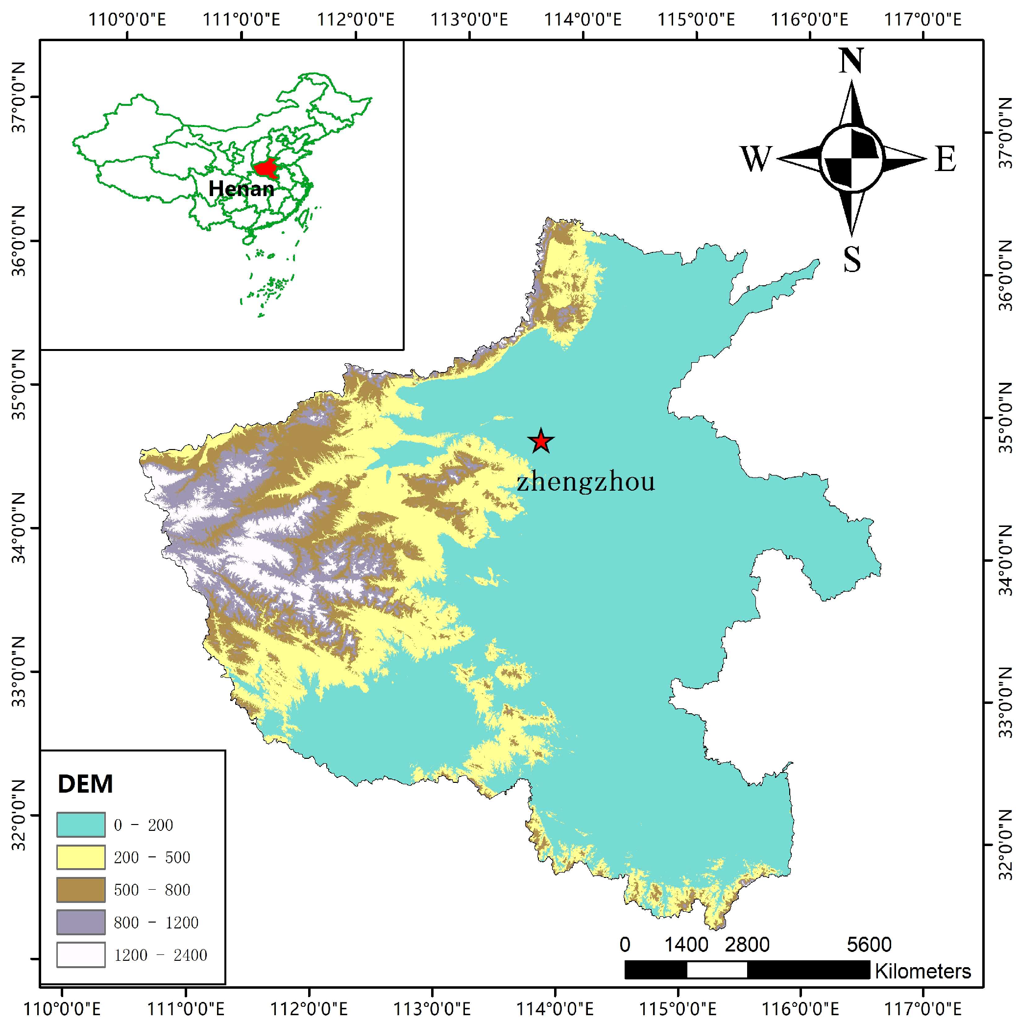
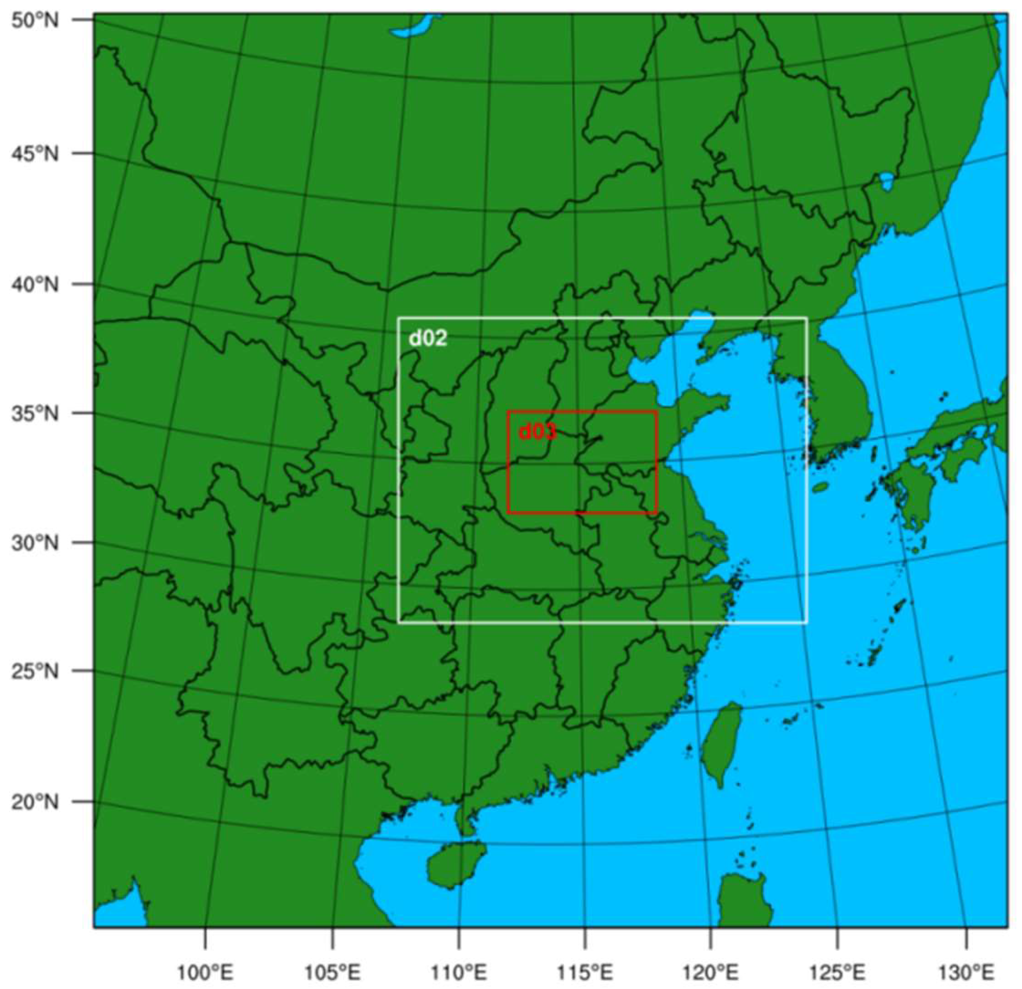
The correction process consists of five distinct steps. Firstly, the study area is determined and the necessary data are prepared. Secondly, the data are processed. Thirdly, a sample database is constructed and the data are standardized. Fourthly, the training, validation, and test datasets are divided. Finally, a DL model based on PBT and GRU is developed to correct the deviations in the precipitation product. Various ML algorithms are introduced and the resulting corrections are compared and evaluated. The specific implementation plan is depicted in Figure 1.

2.2. Study Area

The target area for this study is the city of Zhengzhou (112.70°–114.23° E, 34.27°–34.98° N), which is located in northern Henan Province (Figure 2). Zhengzhou, being situated in the middle latitudes, is prone to frequent incursions of cold air. Additionally, warm and humid air masses can also reach the region during the summer, which often leads to the convergence of warm and cold air masses and subsequently results in intense rainfall events. Additionally, there are multiple indications that China’s climate is undergoing a transitional phase, which may result in a change from low summer rainfall to increased precipitation in the northern regions. Therefore, the selection of Zhengzhou as the study area for this research is highly appropriate. Undoubtedly, this study will serve as a crucial stepping stone toward enhancing severe weather warnings and disaster prevention and mitigation capabilities in the region. It demonstrates a forward-thinking approach with a strategic perspective, setting the stage for future advancements in this field.

2.3. Construction of the Sample Database

The data used in this research consisted of numerical model NWP gridded forecast data and observation data. The observational data in this study were obtained from the Henan Meteorological Bureau. Specifically, we utilized the hourly ground observation data from 2014 to 2022 of Erqi Station (Station No. 57083), located in Zhengzhou, as the sample dataset. The data used in this study were obtained from the mesoscale weather model WRF4.0, a non-hydrostatic model jointly developed by numerous universities and research institutions in the United States [32]. This model features a data assimilation system capable of incorporating meteorological data and executing parallel operations. Moreover, it integrates the latest research findings and advancements from experts and scholars across various fields, providing a solid foundation for both scientific research and practical applications [33]. At the same time, we utilized WRF4.0 to conduct numerical simulations of the weather process. We then compared and analyzed the corrected results of other ML algorithms using the high-resolution forecast results generated by the model. The model configuration settings are listed in

Table 1. Summary of physical parameterizations and other configurations used in simulations.

Mode configurations	Option selection
Nesting ratio	1:3:3, d01 27 km; d02 9 km; d03 3 km
Vertical levels	50 levels
Microphysics	WRF Single-Moment 6-class scheme
Planetary boundary layer	Mellor–Yamada–Janjic scheme
Longwave radiation	RRTM scheme
Shortwave radiation	RRTM scheme
Land surface	Noah land-surface model
Spin-up time	per 6 h

. First, the temporal resolution was set at 6 h, and the horizontal resolution was set at 0.25° × 0.25°. Three nested domains were utilized, with the center of the simulation area located at (34.47° N, 114.21° E), as shown in Figure 3. The grid sizes for the domains were set at 151 × 151, 202 × 151, and 220 × 151. These domains had corresponding grid spacings of 27 km, 9 km, and 3 km, respectively. The model employed 50 layers for the vertical dimension, with a top pressure level of 50 hPa. The physical parameterization schemes used in all the model domains and experiments were the WRF Single-Moment 6-class microphysics scheme [34], the Mellor–Yamada–Janjic planetary boundary layer scheme [35], the rapid radiative transfer scheme (RRTM) [36] and the unified Noah land-surface model [37,38]. All the settings mentioned above are the optimal configurations for this simulation region, as summarized by Liu et al. [39]. Next, all the experiments used NCEP FNL data as input conditions to help observe the changes in the model’s required spin-up times. The time step used for the lateral boundary condition file was one hour. The history output files of each domain were logged hourly.

Given the extensive parameters and high computational power requirements for training the DL model in this study, we select the radar reflectivity factor as the predictive factor. This feature serves as an indicator of the generation and development of convection, as it reflects the reflection of radar waves in various height layers. After the selection of NWP gridded forecast data and observation data, a sample database was generated for the purpose of model training. The database consisted of 54 meteorological variables that were updated on an hourly basis. These data can be classified into eight distinct categories: air pressure (P), visibility (VIS), wind direction (WD), wind speed (WS), air temperature (T), relative humidity (RH), precipitation (P), and NWP (see

Table 2. Categories of meteorological features.

Category	Meteorological Variables
P	‘Sea-level pressure (Pa)’, ‘3 h pressure change (Pa)’, ‘24 h pressure change (Pa)’, ‘Maximum pressure (Pa)’, ‘Time of maximum pressure’, ‘Minimum pressure (Pa)’, ‘Time of minimum pressure’, ‘Ground Pressure (Pa)’.
VIS	‘Visibility (m)’, ‘1 min average Visibility (m)’, ‘10 min average Visibility (m)’, ‘Minimum visibility (m)’, ‘Minimum visibility occurrence time’.
WD	‘2 min average wind direction (°)’, ‘10 min average wind direction (°)’, ‘Maximum wind direction (°)’, ‘Instantaneous wind direction (°)’.
WS	‘2 min average wind speed (m/s)’, ‘10 min average wind speed (m/s)’, ‘Maximum wind speed (m/s)’, ‘Instantaneous wind speed (m/s)’.
T	‘Air temperature (°C)’, ‘Tmax (°C)’, ‘Occurrence time of Tmax (°C)’, ‘Tmin (°C)’, ‘Time of tmin (°C)’, ‘24 h of temperature change (°C)’, ‘Maximum temperature in the last 24 h (°C)’, ‘The lowest temperature in the last 24 h (°C)’, ‘5 cm ground temperature (°C)’, ‘10 cm ground temperature (°C)’, ‘15 cm ground temperature (°C)’, ‘20 cm ground temperature (°C)’, ‘40 cm ground temperature (°C)’, ‘80 cm ground temperature (°C)’, ‘160 cm ground temperature (°C)’, ‘320 cm ground temperature (°C)’, ‘Ground temperature (°C)’, ‘Maximum ground temperature (°C)’, ‘Maximum ground temperature occurrence time’, ‘Minimum ground temperature (°C)’, ‘Minimum ground temperature occurrence time’, ‘Minimum ground temperature in the last 12 h (°C)’.
RH	‘Relative humidity (%)’, ‘Minimum relative humidity (%)’, ‘Minimum relative humidity occurrence time’, ‘Water vapor pressure (Pa)’, ‘Dew point temperature (°C)’.
Pre	‘Hourly precipitation (mm)’, ‘Precipitation in the last 3 h (mm)’, ‘Precipitation in the last 6 h (mm)’, ‘Precipitation in the last 12 h (mm)’, ‘Precipitation in the last 24 h (mm)’.
NWP	‘The radar reflectivity factor’.

for detailed information).

Due to the specific focus of this paper on the correction of hourly precipitation output from the WRF model, we categorized the hourly rainfall into four levels based on the operational practices. By examining the sample distribution presented in

Table 3. Sample sizes of different precipitation levels in 2014–2022.

Precipitation Levels	Precipitation Intensity/mm·h−1	Number of Samples	Sample Ratio/%
No precipitation	[0, 0.1)	72,645	95.25
Weak precipitation	[0.1, 15)	3563	4.67
Moderate precipitation	[15, 30)	40	0.05
Heavy precipitation	[30, ∞)	17	0.02

, it becomes apparent that there exists a significant disparity in the distribution of the hourly rainfall data. Precipitation events of weak intensity are infrequent, constituting a mere 4.74% of the overall distribution. This matter necessitates attention in subsequent iterations of the model training procedures.

2.4. Data Standardization

Due to the wide range of meteorological characteristics encompassed by the input features, each feature possesses distinct dimensions and units. Feeding these features directly into the model introduces complexity to the data processing and may potentially result in model crashes. To mitigate the occurrence of such issues, this study utilized the normalization calculation equation for the purpose of normalization processing, as suggested by Song et al. [40]. This approach uniformly rescales different data values to fit within the standard interval of 0–1. The specific formula can be expressed as follows:

$${\mathrm{x}}^{\ast }=\frac{\mathrm{x}-{\mathrm{x}}_{\mathrm{m}\mathrm{i}\mathrm{n}}}{{\mathrm{x}}_{\mathrm{m}\mathrm{a}\mathrm{x}}-{\mathrm{x}}_{\mathrm{m}\mathrm{i}\mathrm{n}}}$$

(1)

where ${\mathrm{x}}^{\ast }$ represents the standard data, $\mathrm{x}$ represents the original data, ${\mathrm{x}}_{\mathrm{m}\mathrm{a}\mathrm{x}}$ and ${\mathrm{x}}_{\mathrm{m}\mathrm{i}\mathrm{n}}$ represent the maximum and minimum values in the original meteorological dataset. By ensuring that the normalized meteorological sample data falls within the 0–1 standard interval, the training efficiency of the model can be effectively improved, and an efficient calculation process can be ensured when the data are input into the model. Further details can be found in

Table 4. Normalized meteorological features.

Var1 (t − 1)	⋯	Var54 (t − 1)	Var1 (t)	⋯	Var54 (t)
0.774230	⋯	0.525610	0.204615	⋯	0.204606
0.778103	⋯	0.525630	0.204626	⋯	0.204604
0.775722	⋯	0.525688	0.204639	⋯	0.204587
0.775758	⋯	0.525694	0.204653	⋯	0.204589
0.772680	⋯	0.525671	0.204642	⋯	0.204600
0.774621	⋯	0.525621	0.204606	⋯	0.204617
⋮	⋮	⋮	⋮	⋮	⋮
0.777357	⋯	0.525613	0.204637	⋯	0.204681
0.776291	⋯	0.525610	0.204600	⋯	0.204626
0.776006	⋯	0.525660	0.204626	⋯	0.204571
0.777001	⋯	0.525660	0.204589	⋯	0.204606
0.774514	⋯	0.525619	0.204622	⋯	0.204639

.

Considering the inclusion of meteorological features such as the temperature, relative humidity, pressure, wind speed, visibility, and precipitation in the sample database, it is important to note that these features, due to being observed simultaneously, cannot be directly utilized for prediction purposes. In order to ensure precise predictions, it is imperative to establish a correlation between the meteorological characteristics observed in the past and the predictive indicators for the future. Based on the aforementioned considerations, the normalized sample data are structured into time series data. Subsequently, the time series data are shifted backwards, where t represents the current time. The input value is taken as the sample observation data at time t − 1, while the output value is the precipitation data at time t.

Based on the data presented in Table 4, all the sample data are normalized. Specifically, Var1(t − 1), Var2(t − 1), …, and Var54(t − 1) represent the observed values of 54 meteorological variables at time t − 1, while Var1(t), Var2(t), …, and Var54(t) represent the observed values of the same 54 meteorological variables at time t. This study aims to predict future precipitation based on observations at previous times. To achieve this, we retain Var1(t) as the predicted value for the precipitation at time t, and remove the remaining data of Var2(t), Var3(t), …, and Var54(t). The performance of the predictions is evaluated using seven statistical metrics: Probability of Detection (POD), Threat Score (TS), Equitable Threat Score (ETS), Bias Score (BIAS), accuracy, False Alarm Rate (FAR), and Missing Alarm Rate (MAR), which are defined as follows:

$$\mathrm{P}\mathrm{O}\mathrm{D}=\frac{\mathrm{h}}{\mathrm{h}+\mathrm{m}}$$

(2)

$$\mathrm{T}\mathrm{S}=\frac{\mathrm{h}}{\mathrm{h}+\mathrm{m}+\mathrm{f}}$$

(3)

$$\mathrm{E}\mathrm{T}\mathrm{S}=\frac{\mathrm{h}-{\mathrm{h}}_{\mathrm{r}\mathrm{a}\mathrm{n}\mathrm{d}\mathrm{o}\mathrm{m}}}{\mathrm{h}+\mathrm{f}+\mathrm{m}+-{\mathrm{h}}_{\mathrm{r}\mathrm{a}\mathrm{n}\mathrm{d}\mathrm{o}\mathrm{m}}}, {\mathrm{h}}_{\mathrm{r}\mathrm{a}\mathrm{n}\mathrm{d}\mathrm{o}\mathrm{m}}=(\mathrm{h}+\mathrm{f})\times (\mathrm{h}+\mathrm{m})/(\mathrm{h}+\mathrm{m}+\mathrm{f}+\mathrm{c})$$

(4)

$$\mathrm{B}\mathrm{I}\mathrm{A}\mathrm{S}=\frac{\mathrm{h}+\mathrm{f}}{\mathrm{h}+\mathrm{m}}$$

(5)

$$\mathrm{A}\mathrm{c}\mathrm{c}\mathrm{u}\mathrm{r}\mathrm{a}\mathrm{c}\mathrm{y}=\frac{\mathrm{h}+\mathrm{c}}{\mathrm{h}+\mathrm{m}+\mathrm{f}+\mathrm{c}}$$

(6)

$$\mathrm{F}\mathrm{A}\mathrm{R}=\frac{\mathrm{f}}{\mathrm{h}+\mathrm{f}}$$

(7)

$$\mathrm{M}\mathrm{A}\mathrm{R}=\frac{\mathrm{m}}{\mathrm{h}+\mathrm{m}}$$

(8)

In the context of the statistical metrics used to evaluate the performance of the outcomes, the definitions of the contingency table statistics are as follows:

• h: the number of forecasted events that match the actual events.
• m: the number of actual events that were not forecasted.
• f: the number of forecasted events that did not occur in reality.
• c: the number of events that were neither forecasted nor occurred in reality.

These contingency table statistics are used to calculate the statistical metrics, which provide insights into the performance of the correction model.

2.5. Training and Test Dataset

The sample dataset exhibits a significant class imbalance due to the infrequent occurrence of convective weather. Specifically, the number of positive samples representing convective weather with an intensity of weak precipitation (greater than or equal to 0.1 mm/h) is considerably lower than the number of negative samples representing convective weather without precipitation (less than 0.1 mm/h). This particular instance serves as a quintessential illustration of the issue of sample imbalance, as discussed by Krawczyk et al. [41]. To mitigate this concern, a down-sampling technique is utilized to randomly eliminate the surplus samples, taking into account the ratio of positive and negative samples in the dataset. This approach ensures a balanced distribution of positive and negative samples [42].

During the experiment, six distinct ratios of positive and negative samples are chosen, namely 3620:72,645, 1:1, 1:2, 1:3, 2:1, and 3:1. Among the samples, the number 3620 represents the actual count of positive samples, whereas 72,645 represents the actual count of negative samples. When the PBT-GRU model is trained without any adjustments to the sample quantity, the Probability of Detection (POD), accuracy, and Threat Score (TS) scores are 0.6237, 0.6114, and 0.5982, respectively. Based on the distribution of positive samples in the original dataset, we employ a random selection process to obtain negative samples in order to maintain a balanced ratio of positive to negative samples at 1:2 and 1:3. Subsequently, we utilize the down-sampling technique to adjust the number of negative samples, resulting in a 2:1 and 3:1 ratio of positive to negative samples, respectively. The PBT-GRU model is subsequently trained, and the findings from the experiments are presented in

Table 5. Training results with different positive and negative samples.

Experimental Category	Proportion of Positive and Negative Samples in the Training Set	Accuracy	POD	TS
Practical sampling test	3620:72645	0.6114	0.6237	0.5982
Resampling test 1	1:1	0.8718	0.8921	0.7766
Resampling test 2	1:2	0.7023	0.6715	0.6434
Resampling test 3	1:3	0.6938	0.6523	0.6235
Resampling test 4	2:1	0.8546	0.9468	0.7512
Resampling test 5	3:1	0.8549	0.9657	0.7567

. When the ratio of positive and negative samples is balanced at 1:1, the accuracy and True Skill (TS) of hourly precipitation exhibit their highest values. However, the Probability of Detection (POD) score for the hourly precipitation is slightly lower. As the ratio of positive and negative samples increases to 2:1 and 3:1, there is an observed increase in the number of positive samples. This leads to higher Probability of Detection (POD) scores, while the accuracy and True Skill (TS) scores show a slight decrease. Conversely, when the ratio of positive and negative samples is 1:2 and 1:3, there is an increase in the number of negative samples, resulting in a notable decrease in the scores for the Probability of Detection (POD), accuracy, and TS (Threat Score). In conclusion, in order to enhance the prediction performance, we have determined that a 1:1 ratio of positive and negative samples is the optimal choice.

To obtain objective and fair experimental results, we employ random deletion to balance the number of positive and negative samples in the original dataset. This approach can ensure that the sample size is controlled and balanced. We then divide all the positive and negative samples into three subsets: the experimental training dataset, validation dataset, and test dataset. The training dataset constitutes 80% of the total samples, the validation dataset comprises 10%, and the remaining 10% serves as the test dataset.

3. Correction Model Construction Based on PBT and GRU

3.1. Dataset Dimensionality Reduction by RF

The high dimensionality and complexity of features in ML frequently result in reduced computational efficiency and heightened operating costs, which are detrimental to business-oriented applications. In the context of nonlinear complex feature spaces and vast high-dimensional data, the task of eliminating redundant and irrelevant feature values from input features has emerged as a critical concern in the field of ML. Feature filtering and dimensionality-reduction techniques are employed to identify and retain input features that possess high importance and contain rich information. This process ultimately improves the model’s ability to extract and refine relevant information. Random Forest (RF) is an ML algorithm that utilizes bootstrapping resampling to randomly select data for constructing resampled samples. The approach employs random splitting to construct multiple decision trees for each sample, and it subsequently aggregates the decision trees to derive the final prediction outcome via a voting mechanism. Random Forest (RF) is a commonly employed technique for feature selection. It operates by assessing the importance of each feature, ranking them based on their calculated importance, and subsequently filtering out the most significant ones. This is particularly valuable in scenarios where a substantial number of features are involved in classification or regression tasks. It is common for many features to exhibit high correlation and dimensionality issues. Incorporating these features into the model can have a significant impact on the accuracy of model training and prediction. By utilizing the Random Forest (RF) algorithm, an importance analysis can be conducted to determine the significance of each predictor and establish a prioritized ranking. The fundamental principle entails the quantification of the contribution made by each feature in every tree within the Random Forest. These values are then averaged and compared to determine the relative contributions among the features. Typically, the Gini index or Out-of-Bag (OOB) error rate can be employed as an evaluation metric. In this study, our primary focus is on the utilization of the Gini index as a means of assessment, as discussed by Breiman [43], Robin et al. [44], and McGovern et al. [45]. Here, we denote the Variable Importance Measure (VIM) as the score reflecting the importance of the variables, while GI represents the Gini index. Assuming there are J features, I decision trees, and C categories, the Gini index of node q in the i-th tree is calculated as follows:

$${\mathrm{G}\mathrm{I}}_{\mathrm{q}}^{\left(\mathrm{i}\right)}=\sum _{\mathrm{c}=1}^{\left|\mathrm{C}\right|}\sum _{{\mathrm{c}}^{\prime }\ne \mathrm{c}}{\mathrm{P}}_{\mathrm{q}\mathrm{c}}^{\left(\mathrm{i}\right)}{\mathrm{P}}_{\mathrm{q}{\mathrm{c}}^{\prime }}^{\left(\mathrm{i}\right)}=1-\sum _{\mathrm{c}=1}^{\left|\mathrm{C}\right|}{\left({\mathrm{P}}_{\mathrm{q}\mathrm{c}}^{\left(\mathrm{i}\right)}\right)}^2$$

(9)

Among them, C represents the categories, and ${\mathrm{P}}_{\mathrm{q}\mathrm{c}}$ denotes the proportion of category c at node q. The change in the Gini index for a feature is given by:

$${\mathrm{V}\mathrm{I}\mathrm{M}}_{\mathrm{j}}^{\left(\mathrm{G}\mathrm{i}\mathrm{n}\mathrm{i}\right)\left(\mathrm{i}\right)}=\sum _{\mathrm{q}\in \mathrm{Q}}{\mathrm{V}\mathrm{I}\mathrm{M}}_{\mathrm{j}\mathrm{q}}^{\left(\mathrm{G}\mathrm{i}\mathrm{n}\mathrm{i}\right)\left(\mathrm{i}\right)}$$

(10)

Suppose there are I trees in the Random Forest (RF), then:

$${\mathrm{V}\mathrm{I}\mathrm{M}}_{\mathrm{j}}^{\left(\mathrm{G}\mathrm{i}\mathrm{n}\mathrm{i}\right)}=\sum _{\mathrm{i}=1}^{\mathrm{I}}{\mathrm{V}\mathrm{I}\mathrm{M}}_{\mathrm{j}}^{\left(\mathrm{G}\mathrm{i}\mathrm{n}\mathrm{i}\right)\left(\mathrm{i}\right)}$$

(11)

Finally, normalization is performed:

$${\mathrm{V}\mathrm{I}\mathrm{M}}_{\mathrm{j}}^{\left(\mathrm{G}\mathrm{i}\mathrm{n}\mathrm{i}\right)}=\frac{{\mathrm{V}\mathrm{I}\mathrm{M}}_{\mathrm{j}}^{\left(\mathrm{G}\mathrm{i}\mathrm{n}\mathrm{i}\right)}}{{\sum }_{{\mathrm{j}}^{\prime }=1}^{\mathrm{J}}{\mathrm{V}\mathrm{I}\mathrm{M}}_{{\mathrm{j}}^{\prime }}^{\left(\mathrm{G}\mathrm{i}\mathrm{n}\mathrm{i}\right)}}$$

(12)

The specific steps involved in this process are as follows. Firstly, the feature importance needs to be calculated for all the features. Subsequently, these features are ranked in descending order based on their importance. When provided with a predetermined threshold for the proportion of features to be rejected, this threshold can be utilized as a criterion to eliminate excessive features by considering their importance. Repeat steps 1 and 2 on the remaining feature dataset until the desired number of features has been selected. The feature dataset with the lowest Out-of-Bag error rate, which corresponds to the selected feature set, should be chosen as the input for the model [43,44].

Through the implementation of RF dimensionality reduction, we have identified the nine most significant features, which collectively account for an importance score of 0.853. The specific findings are displayed in Figure 4 and

Table 6. Results of feature value importance analysis.

Serial Number	Feature Value	Importance	Cumulative Importance
1	Radar reflectivity factor	0.327	0.327
2	3 h of precipitation	0.213	0.540
3	Automatic observation of the minimum visibility	0.109	0.649
4	6 h of precipitation	0.063	0.712
5	Artificial visibility	0.043	0.755
6	12 h of precipitation	0.041	0.796
7	Automatic observed 10 min average horizontal visibility	0.026	0.822
8	Automatic observed 1 min average horizontal visibility	0.017	0.839
9	Extreme wind speed	0.014	0.853

. The results show that for the feature of convective weather, the importance of the features ranked by the machine-learning method is largely consistent with the subjective understanding of forecasters, for example, the radar reflectivity factor is the most important predictive factor for judging short-term heavy precipitation. Through the analysis of the objective ranking of these features, some useful inspiration can also be obtained. For example, automatic observation of the minimum visibility is an important factor in predicting precipitation. As the intensity and duration of precipitation can significantly modulate visibility, consistent and stable rainfall can easily trigger a long low-visibility scenario, and the sudden heavy precipitation is an important factor inducing the sharp decrease in visibility. With the increase in rainfall, the visibility changes from a rapid decline to a slow decline and there exists an inflection point [46]. Therefore, the automatic observation of the minimum visibility is important. which can be used more in business.

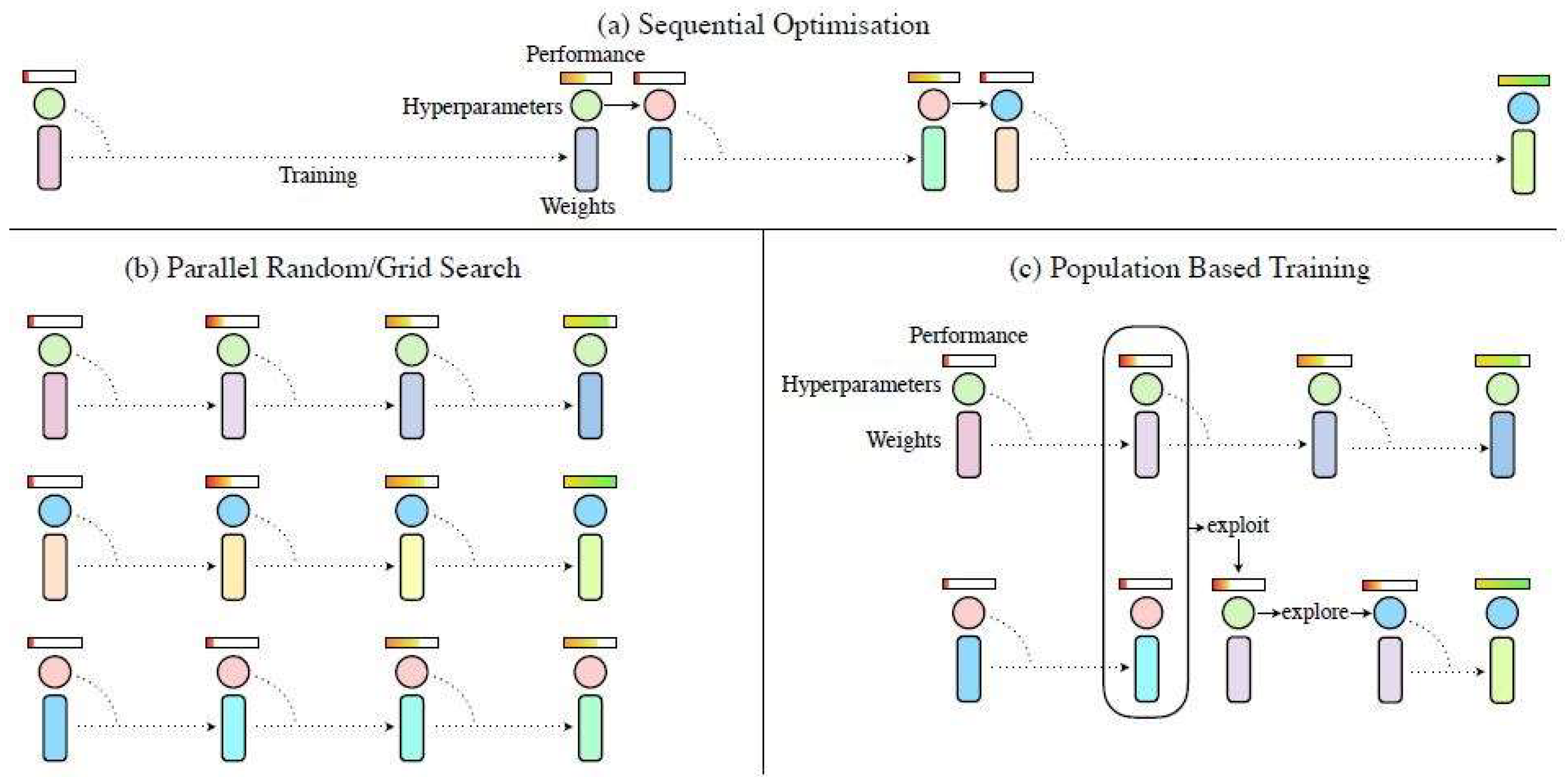
3.2. The PBT Optimization Algorithm

The training process for ML models encompasses a multitude of parameters and hyperparameters that exert a substantial influence on the ultimate efficacy of these models. Traditionally, the manual adjustment of these parameters and hyperparameters has been common practice. However, this approach is characterized by its time-consuming and labor-intensive nature, and it does not provide a guarantee of achieving an optimal solution. Consequently, automatic adjustment methods have emerged as the predominant approach. Parallel search and sequence optimization are two distinct approaches utilized in the field of automatic tuning, each comprising a variety of individual methods. In the context of optimization algorithms, parallel search refers to the simultaneous training of multiple sets of parameters. This approach utilizes various techniques, including random search and grid search, to efficiently explore the parameter space. One limitation of this approach is the inefficient utilization of optimization information across parameters. On the contrary, sequence optimization aims to optimize the parameters by employing a series of iterative attempts, without the inclusion of parallel operations. This methodology encompasses various strategies, such as Bayesian optimization and manual parameter tuning. Nevertheless, it is imperative to take into account that certain parameters, such as the degree of exploration and the learning rate, experience continuous fluctuations throughout the training process of the model. The conventional approach involves initially establishing predetermined values and subsequently modifying them in response to various scenarios. Unfortunately, this approach frequently does not result in the optimal parameter value. In conclusion, the careful selection and optimization of parameters and hyperparameters play a crucial role in determining the overall performance of ML and DL models. While conventional manual adjustment techniques are laborious and time-consuming, automatic tuning methods provide more efficient solutions, albeit with inherent limitations.

The Population-Based Training (PBT) method has been shown to be effective in automating and optimizing hyperparameters [47]. Figure 5 presents a visual representation of the main differences among the PBT, sequence optimization, and parallel search methods. (A) Sequential optimization necessitates the completion of multiple training runs, which may include early stopping. Afterward, fresh hyperparameters are chosen, and the model is retrained from the beginning utilizing the newly selected hyperparameters. The aforementioned process is inherently sequential, leading to prolonged durations for hyperparameter optimization. However, it utilizes minimal computational resources. (B) In contrast, the parallel random/grid search of hyperparameters entails the simultaneous training of multiple models with varying weight initializations and hyperparameters. The objective is to identify the most optimized model among the available options. This approach entails the need for a solitary training session; however, it demands the utilization of additional computational resources to simultaneously train multiple models. The PBT algorithm integrates the advantages of sequence optimization and parallel search. Initially, the PBT algorithm employs a random initialization process to generate multiple models. During the training process, checkpoints are automatically generated at regular intervals. Each model autonomously adapts its behavior in response to the performance of other models. If a model exhibits encouraging outcomes, the training process persists. Conversely, in the event that a model’s performance is deemed unsatisfactory, its parameters are substituted with those derived from a model that exhibits superior performance. Additionally, in order to further explore the parameter space, random disturbances are introduced during the training process. Checkpoints are established through manual configuration, whereas disturbances are induced by introducing noise. In summary, the PBT method combines the advantages of the sequence optimization and parallel search methods, facilitating the efficient and effective adjustment and optimization of hyperparameters. The PBT algorithm demonstrates dynamic adaptation to enhance the overall training outcomes by employing checkpoint generation, model evaluation, and parameter replacement techniques [47].

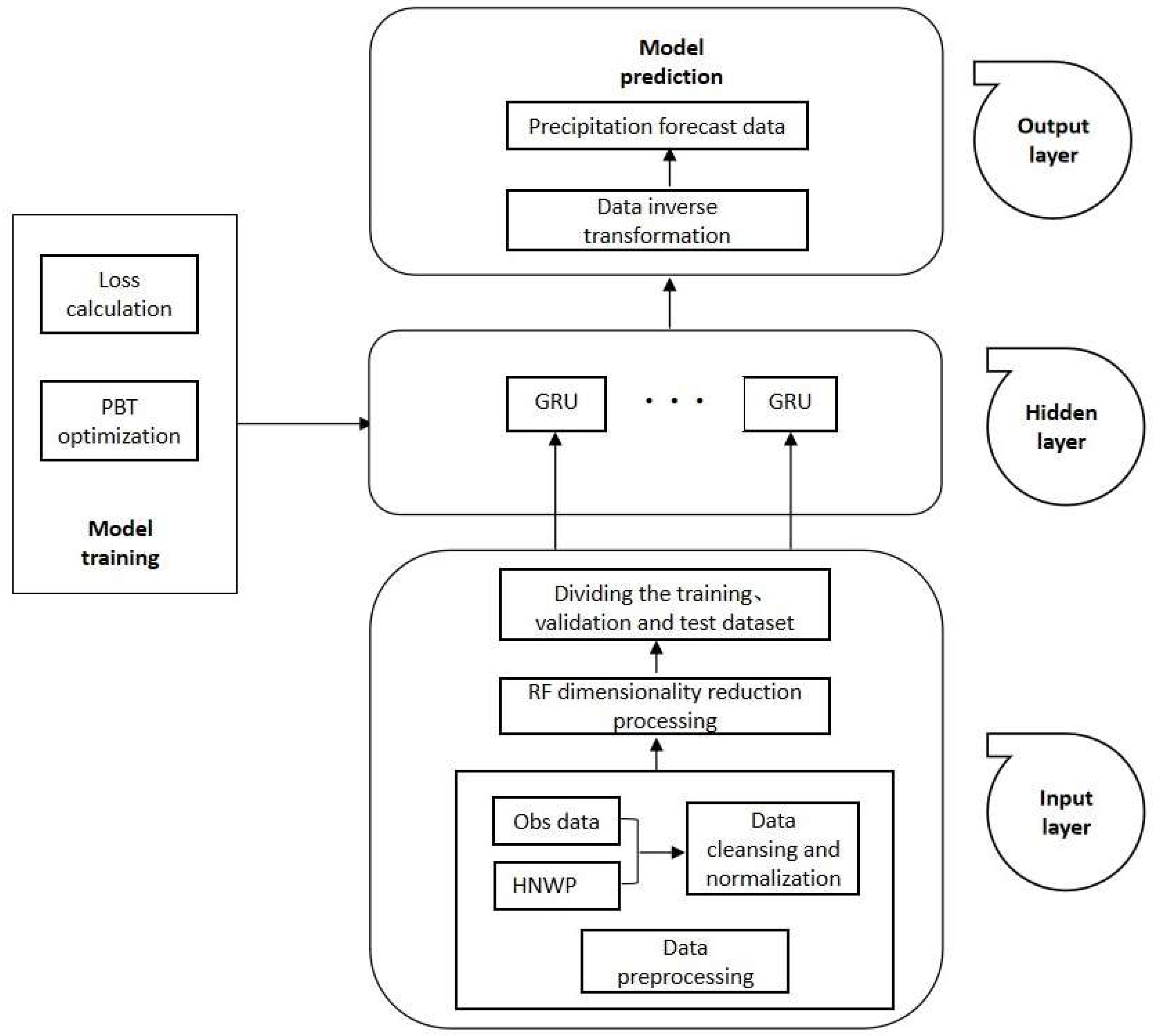
3.3. Construction of the Model

This paper introduces the development of a DL model called PBT-GRU. The PBT-GRU uses the sequence data from ground observations and numerical model grid points as input. Firstly, to optimize the efficiency, preprocessing techniques such as data normalization and cleaning are employed on the initial meteorological data. After completing the above operations, dimensionality reduction of the initial dataset is performed using the Random Forest algorithm. Secondly, two GRU layers are used to extract the time-varying features of the sequence data, in which the first GRU layer, containing 128 neurons, is set to return the complete sequence, and the second GRU layer, containing 64 neurons, is set not to return the complete sequence, and the activation function of the two GRU layers is ReLU. Finally, the predicted precipitation size is obtained from the output of the two dense layers. The PBT-GRU model contains two GRU layers and two fully connected layers, and through the stacking of these layers and the processing of the activation function, the model can learn the features of the input data and output the prediction results (as illustrated in Figure 6). Interpolation is necessary to obtain the meteorological element values of the forecast station, as the forecast station and model grid points are not located at the same point. This is because the grid point element values near the forecast station need to be interpolated. Given the potential error introduced by interpolation, we employ bilinear interpolation as a means to mitigate the influence of this error. This approach allows us to generate a sample database for training the model. In order to ensure the comparability of different models, both the PBT-GRU model and other ML models undergo a reconstruction of the sample dataset. By taking into account the evolutionary patterns and characteristics of weather systems, the incorporation of this factor allows the model to capture the fundamental causal connections between precipitation and other forecast attributes in the long-term series. The proposed PBT-GRU model effectively combines the benefits of Population-Based Training and the GRU architecture. Through the implementation of efficient preprocessing techniques and the incorporation of NWP gridded forecast data and observation data, the model significantly improves its predictive capabilities by accurately capturing the complex interplay between precipitation and other features.

The model training process employs the early stop strategy, with the iteration period (Epoch) set to 300. If the loss does not decrease for more than 10 epochs, the operation is automatically terminated. A batch size of 16 is used. The loss function selected for minimization during training is the mean squared error (MSE). The formula is as follows:

$$\mathrm{M}\mathrm{S}\mathrm{E}=\frac{1}{\mathrm{m}}\sum _{\mathrm{i}=1}^{\mathrm{m}}{({\mathrm{y}}_{\mathrm{i}}^{\prime }-{\mathrm{y}}_{\mathrm{i}})}^2$$

(13)

where m represents the training sample size, ${\mathrm{y}}_{\mathrm{i}}$ represents the actual value, and ${\mathrm{y}}_{\mathrm{i}}^{\prime }$ represents the predicted value. Statistical measures, including the correlation coefficient (r), standard deviation (${\mathsf{\sigma }}_{\mathrm{n}}$), and root mean square error (RMSE), are used to assess the model performance.

3.4. Experimental Setup

To evaluate the efficacy of the different models, we utilized a range of methods, including Random Forest (RF), Support Vector Machine (SVM), K-Nearest Neighbor (KNN), Gradient-Boosting Decision Tree (GBDT), and PBT-GRU. The objective was to enhance the accuracy of the precipitation forecasts generated by the WRF model. These refined outputs were subsequently compared with the original predictions from the WRF model for the purpose of comparison. The input dataset utilized in our study encompassed historical data from the years 2014 to 2022. In our approach, we considered an optimal ratio of 1:1 for positive to negative samples. Given that we had 3620 positive samples, we set an equal number of negative samples, yielding a total of 7240 samples. We segmented this dataset as follows: 80% (that is, 5792 samples) served as our training dataset. The remaining dataset was equally split into two subsets: 10% (or 724 samples) formed our validation dataset, while another 10% were used for the test dataset. We selected nine features identified through the RF screening. It is important to note that the distribution for the training, validation, and test datasets remained consistent across the different models.

4. Results and Discussion

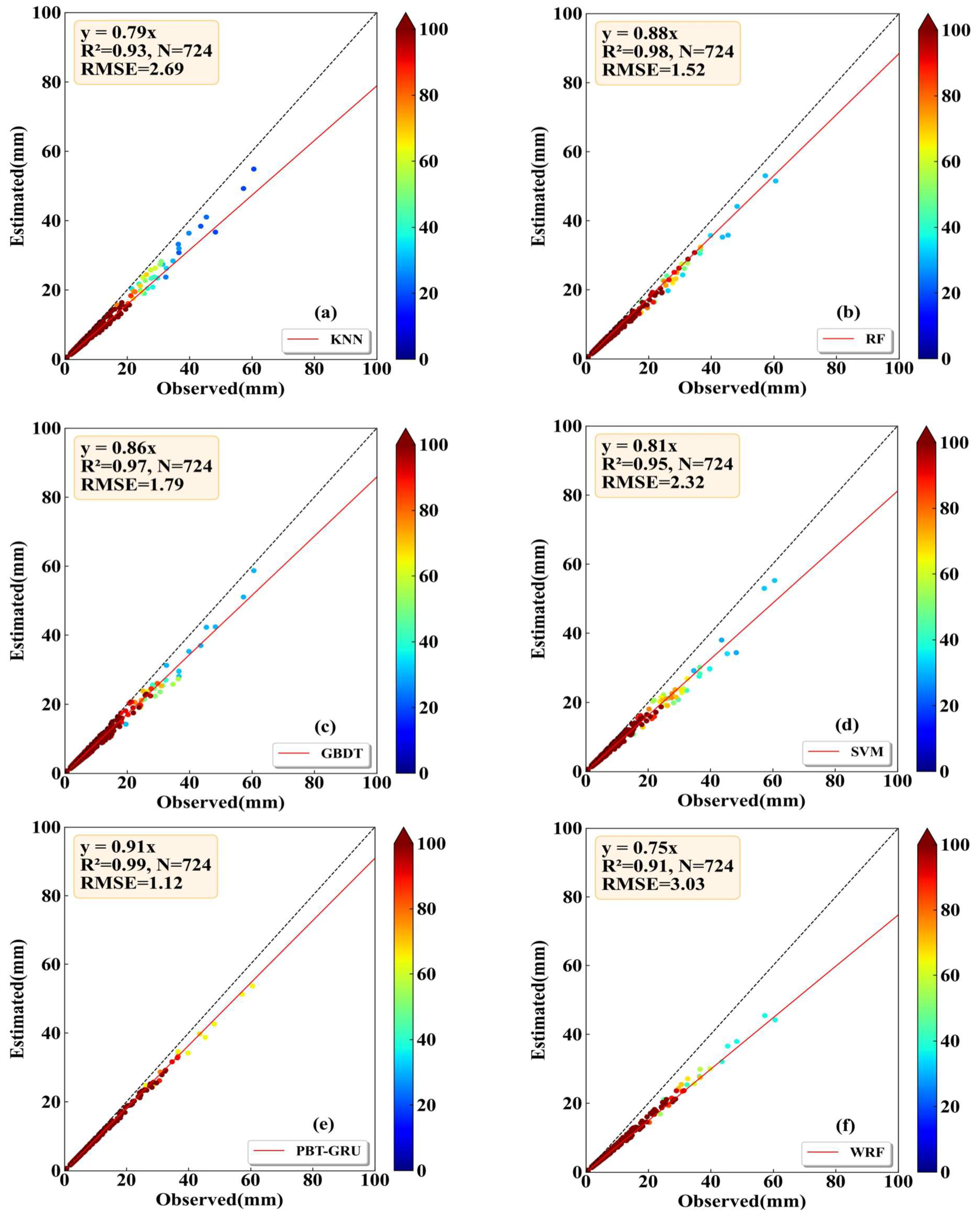
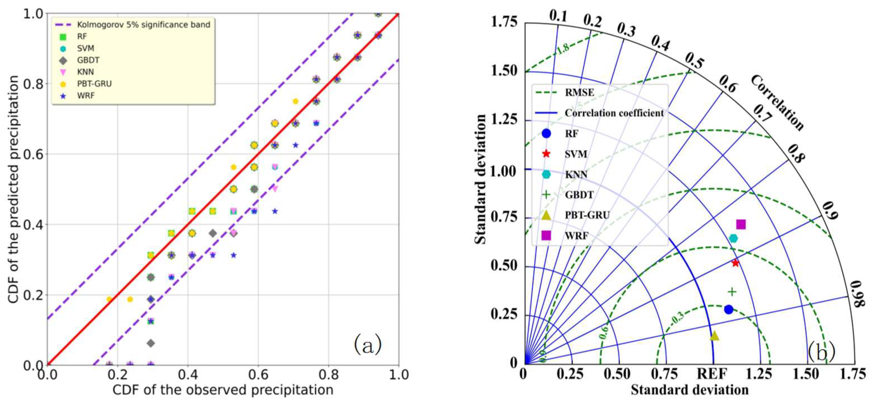
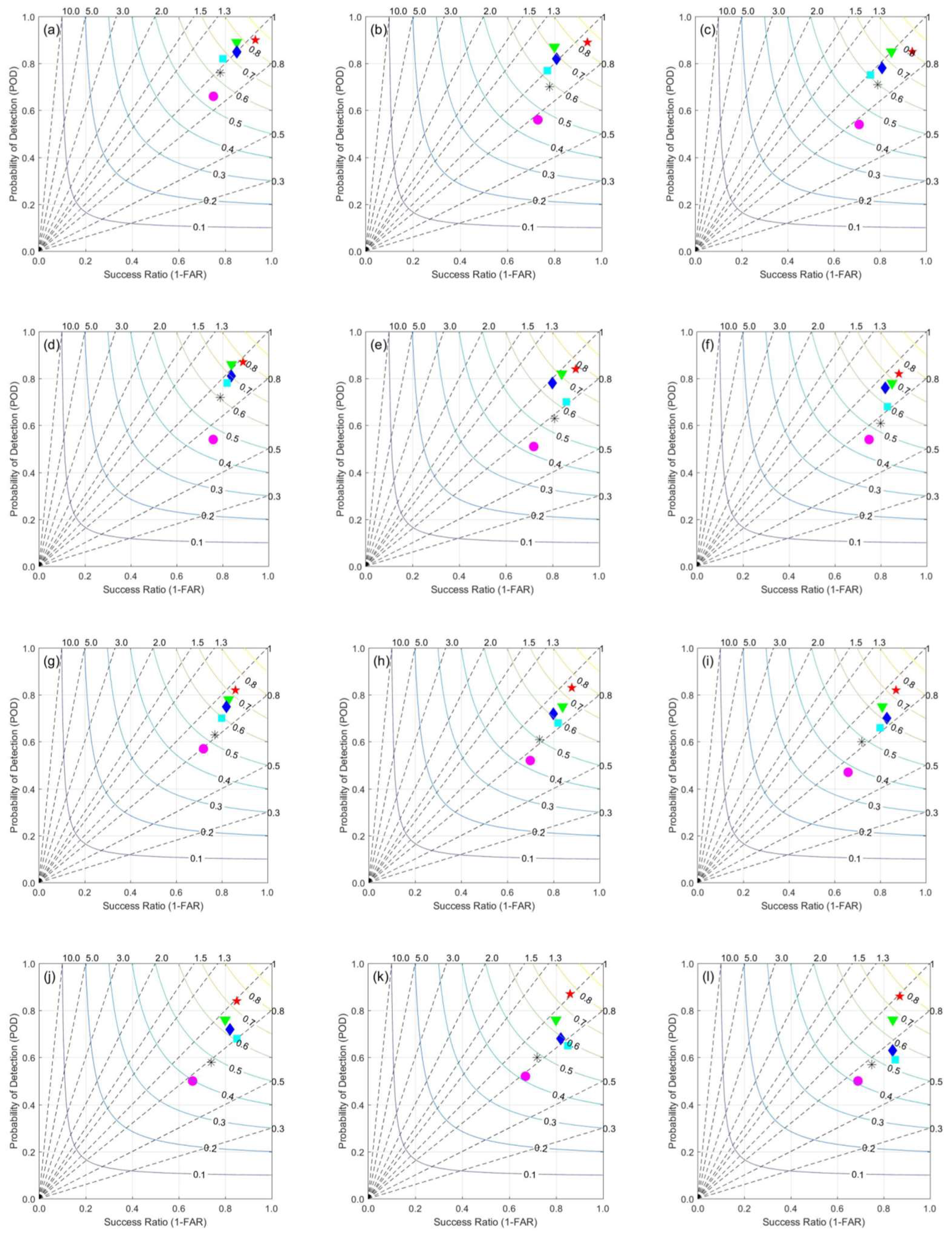
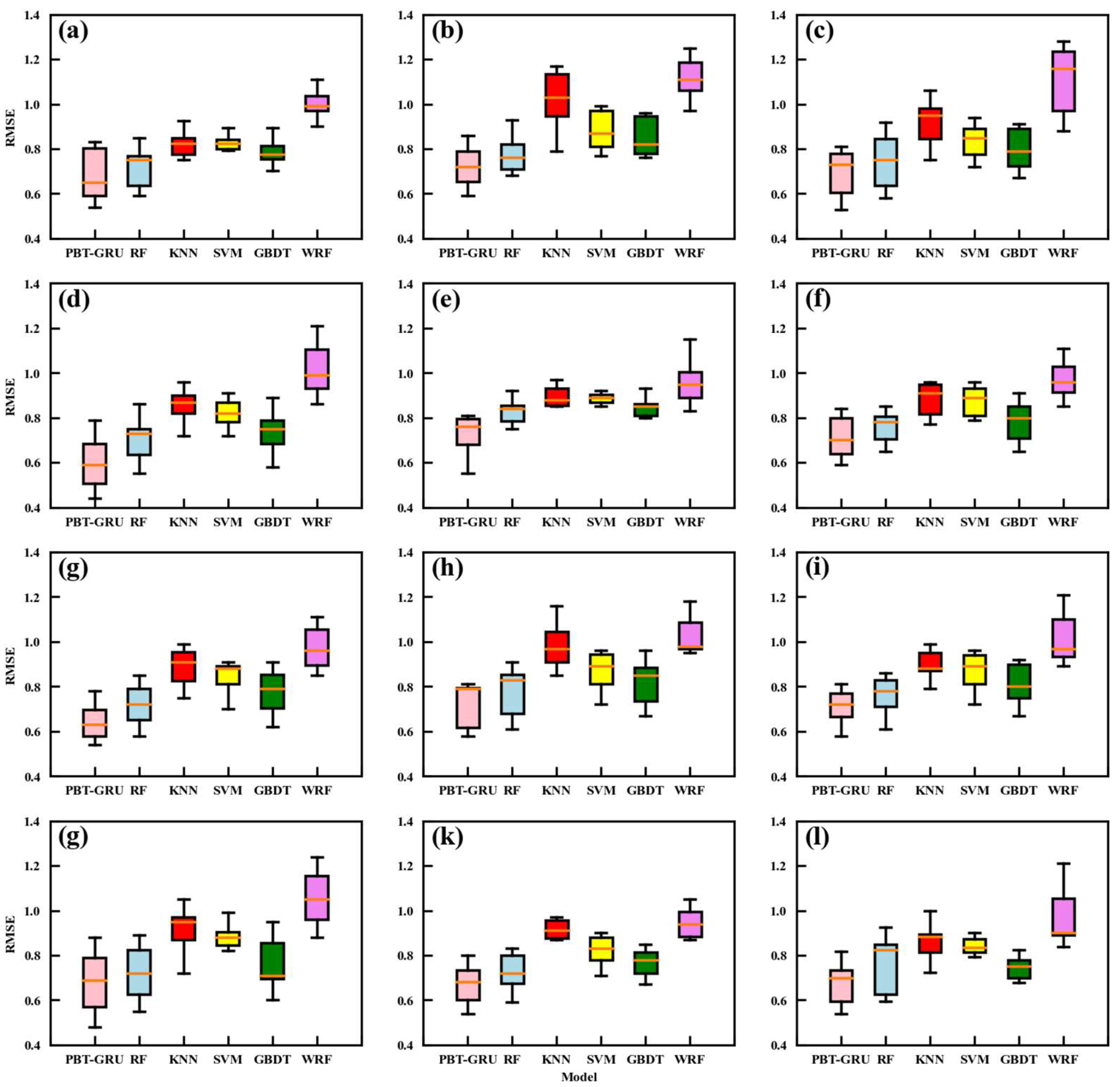
4.1. Comparison with Other ML Methods

To investigate the performance of the PBT-GRU model, we used scattered density plots to compare its performance with the other five models: RF, SVM, KNN, GBDT and WRF. The results are shown in Figure 7. It can be see that the SVM and KNN methods resulted in subpar precipitation corrections, as evidenced by their relatively high RMSE values of 2.32 mm and 2.69 mm, respectively. Compared to the WRF model, these figures represent reductions of 23.43% and 11.22%. Additionally, the correlation coefficients between the corrected and actual precipitation were low due to the more dispersed distributions. On the contrary, RF and GBDT methods demonstrated superior performance in precipitation correction. They achieved smaller RMSE values between the corrected and actual rainfall, reaching 1.52 mm and 1.79 mm, respectively, representing reductions of 49.83% and 40.92% when compared with the WRF model. These methods also exhibited stronger correlations, indicated by the higher correlation coefficients, suggesting concentrated distributions of corrected rainfall and actual precipitation errors. However, despite the promising results obtained by the RF and GBDT methods, the PBT-GRU model proposed in this study outperformed them. The distribution of the corrected and actual precipitation using the PBT-GRU method was notably more concentrated on the 1:1 line, leading to the smallest overall error. Specifically, the RMSE value for the PBT-GRU model was merely 1.12 mm, marking reductions of 63.04%, 51.72%, 58.36%, 37.43%, and 26.32% in comparison to the WRF, SVM, KNN, GBDT, and RF models, respectively. Furthermore, it reached an impressive correlation coefficient of approximately 99% between the corrected precipitation and the actual data. Based on this evidence, it is clear that the PBT-GRU model substantially surpasses traditional ML algorithms such as SVM, KNN, GBDT, and RF in the context of precipitation correction.

To further investigate the performance of the PBT-GRU model, we compared it with the other five models using the cumulative distribution probability scatter plots and Taylor plots, and the results are shown in Figure 8. From the data provided in the figure, it is evident that the PBT-GRU model outperformed the other models significantly. It exhibited a standard deviation of 1.02 and a correlation coefficient of 0.99. Following closely behind as the second most accurate model is the RF model, boasting a standard deviation of 1.12 and a correlation coefficient of 0.97. The WRF model demonstrated the weakest performance, with a standard deviation and correlation coefficient of 1.30 and 0.85, respectively. The accuracy metrics of the SVM, GBDT, and KNN models fell between those of the superior (PBT-GRU and RF) and inferior (WRF) models. Specifically, their standard deviations and correlation coefficients were recorded as follows: SVM—1.24 and 0.91; GBDT—1.15 and 0.94; KNN—1.26 and 0.87. In conclusion, the PBT-GRU model held a distinct advantage due to its ability to effectively extract the development characteristics of convective weather, thereby achieving superior precipitation correction.

4.2. Individual Case Forecast Evaluation

4.2.1. Spatial Distribution

In July 2021, seven individual convective weather events occurred in the Zhengzhou area, characterized by thunderstorms and short-term heavy precipitation, In order to assess and analyze the accuracy of the various models, we chose the forecast results of these cases for evaluation. The TS (Figure 9) and RMSE (Figure 10) distribution of precipitation of the 6 models at 12 stations in Zhengzhou show that the correction effect of the PBT-GRU model is better than the other ML models. At most stations, the TS of the precipitation forecast by WRF is between 40% and 55%, and RMSE value is mostly between 1 mm and 1.3 mm. After the PBT-GRU and other models are corrected, the forecast accuracy of the corrected precipitation is greatly improved. As can be seen from Figure 9 and Figure 10, the TS of PBT-GRU is as high as 80%, and the RMSE is as low as 0.6 mm. The TSs of the RF, SVM, GBDT, and KNN models fall between the PBT-GRU and WRF forecasts. The performances of the corrected precipitation are not as good as the PBT-GRU, with their TS and RMSE recorded as follows: RF: 70–78% and 0.70 mm–0.80 mm, SVM: 60–70% and 0.78 mm–0.95 mm; GBDT: 65–74% and 0.75 mm–0.90 mm, KNN: 55–65% and 0.85 mm–1.00 mm. From the above analysis, it can be concluded that the PBT-GRU model performs the best, followed by RF, GBDT, SVM, and KNN.

In order to evaluate the variability of the errors across the different models, boxplots were utilized as a convenient method to summarize the data from all 12 stations. As depicted in Figure 11, the PBT-GRU model exhibited more accurate results compared to the other models. Its difference between the observed precipitation and the predicted precipitation was minimal, resulting in the highest TS value of 0.82 and the lowest RMSE value of 0.43 mm (Figure 10). These values were significantly superior to those of the other models. For the RF and GBDT models, the difference between the observed precipitation and the predicted precipitation was not significant and both showed better performance than the KNN and SVM models. Overall, the PBT-GRU model showed the best performance, with higher accuracy for all stations, and the KNN and SVM models illustrated the lowest performance among the other models and approaches. However, it was difficult to evaluate the model’s stability due to the few individual cases.

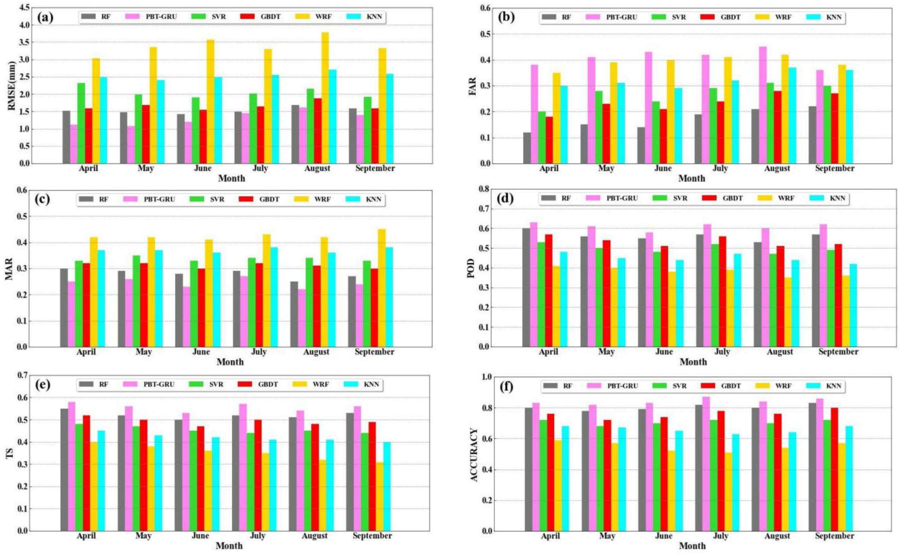
4.2.2. Temporal Variations

Figure 12 depicts the corrections in the diurnal variations offered by the diverse models in July 2021, and it also shows the diurnal fluctuation in precipitation in the initial WRF forecast. The precipitation forecast by the original WRF weather prediction model exhibits noticeable inaccuracies. As can be seen from the figure, the WRF’s precipitation forecast displays a distinct diurnal variation trait, characterized by substantial discrepancies between the early morning and afternoon hours, namely between 9:00 am and 13:00 pm (Figure 12f). This indicates that the WRF’s precipitation forecast tends to be inaccurate and displays significant errors in the diurnal variation.

After the WRF’s precipitation forecast underwent correction, the diurnal variation error was considerably lessened (Figure 12a–e). Initially, the mean precipitation corrected through the PBT-GRU model aligns well with the actual average precipitation trajectory, with a minimal error and being devoid of diurnal variation (Figure 12e). This suggests that the adjusted and actual distributions of precipitation are in agreement. However, the correction performed between 9:00 am and 13:00 pm during January 2021 did not yield satisfactory results. This could be attributed to the inadequate generalization abilities of the training model and the excessive volatility of the actual precipitation at these specific times. Based on the above comparative analysis, it can be inferred that the PBT-GRU model outperforms the other models.

4.3. Stability Analysis of the Proposed Models

The preceding results presented the visualized outcomes of the various correction methods, which may not fully prove the stability of the different approaches. To further evaluate the stability of the various ML models, we compared their performance on strong convective weather forecasting during the flood season (April–September) from 2020 to 2022 by using six evaluation metrics: RMSE, FAR, MAR, POD, TS, and accuracy. The specific results are presented in Figure 13. This comprehensive analysis provides a more accurate assessment of the stability of the different models.

The RMSE values of the five ML models were lower than that of the WRF model, with the PBT-GRU model having the smallest RMSE of 1.12 mm. This represented a 63.04% reduction in the RMSE compared to the output precipitation of the WRF model. From the perspective of solving regression problems, the model effectively corrected the deviation in precipitation predicted by the numerical forecast model. In comparison to the other ML algorithms, the accuracy of the PBT-GRU model showed a significant improvement, demonstrating the stability of DL methods for nonlinear problems such as precipitation, often achieving superior application results.

The FAR and MAR are two important indicators for evaluating precipitation forecasting accuracy, reflecting the false and missing alarm rates, respectively. As shown in the figure, the FAR of the PBT-GRU model was higher than that of all the other models, while its MAR was lower than that of all the other models. This situation might be due to the fact that while the PBT-GRU model effectively fits precipitation, it also has side effects, leading to precipitation forecasts in the absence of actual precipitation. The FAR and MAR values obtained by the other four ML algorithms were lower than those of the WRF model, indicating that these ML methods can reduce the false and missing rates of the WRF model precipitation forecasts to a certain extent.

Finally, the POD, TS and accuracy scores of the five ML models were significantly higher than those of the WRF model, with the PBT-GRU model achieving the best performance among all the models. These results indicate that the PBT-GRU model exhibits an ideal performance in correcting precipitation forecasts from the WRF model, outperforming other ML methods in terms of the precipitation correction.

5. Summary

In this study, we constructed a DL model based on PBT and GRU (PBT-GRU) for correcting the precipitation deviation predicted by the WRF model. Subsequently, we employed ML algorithms such as RF, SVM, KNN, and GBDT to compare with the corrected results of the PBT-GRU model. The main conclusions drawn from this research are as follows:

(1)

The sample balancing experiment results revealed that when the ratio of positive and negative samples was 1:1, both the accuracy and TS scores reached their highest values, while the POD score was slightly lower. As the number of positive samples increased, the POD score improved, yet the accuracy and TS scores slightly decreased. Conversely, when the number of negative samples increased, all three scores, namely the POD, accuracy, and TS, experienced a significant decline with the increase in negative samples.

(2)

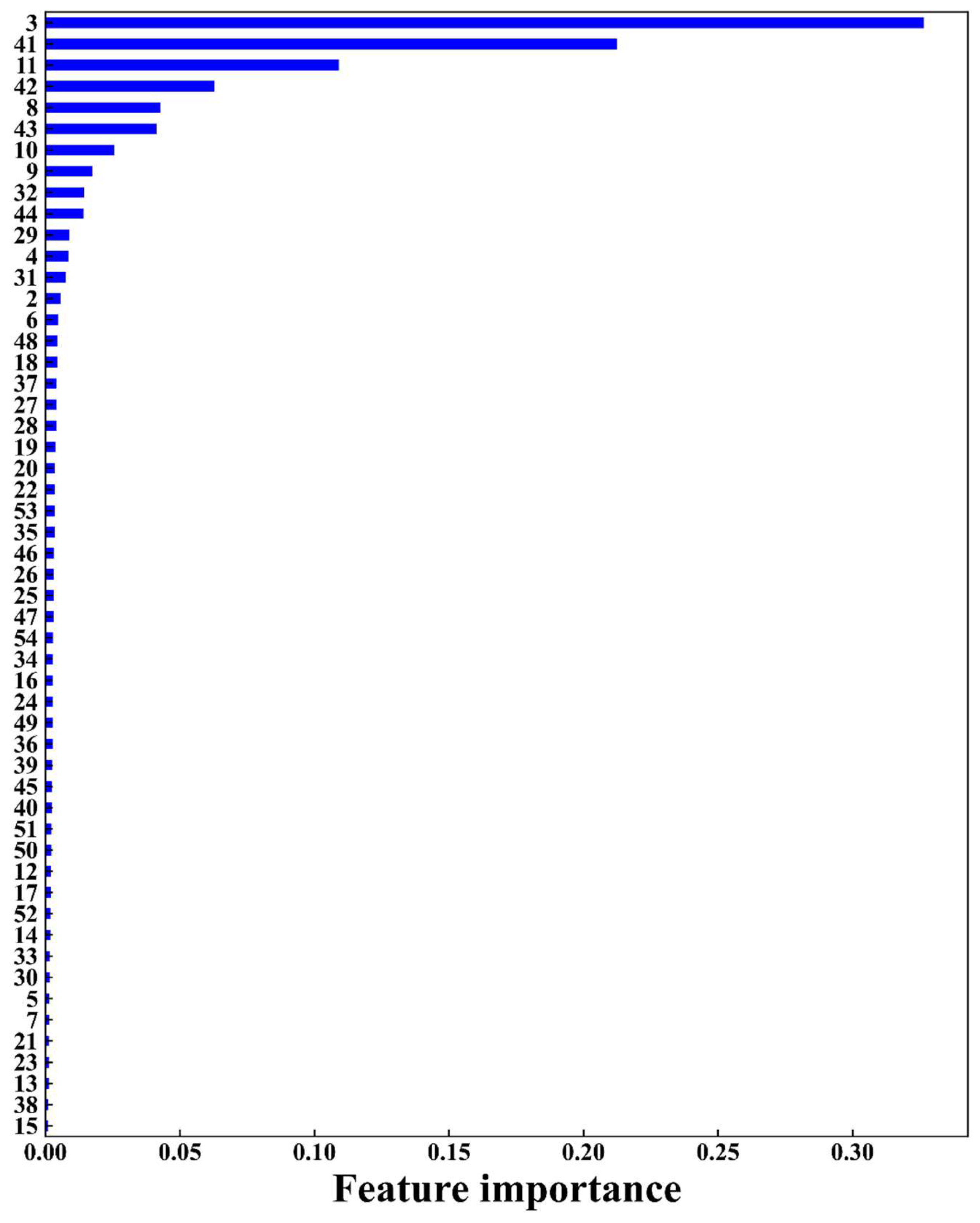
To optimize the model’s performance, we utilized RF to evaluate the significance of various forecast features. As a result, nine key features were identified and selected, including radar reflectivity factor, 3 h precipitation, automatic observation of minimum visibility, 6 h precipitation, artificial visibility, 12 h precipitation, automatic observation of 10 min average visibility, automatic observation of 1 min average visibility, and maximum wind speed. By incorporating these features, the model’s input size was significantly reduced, leading to improved computational efficiency.

(3)

Combining the advantages of PBT and GRU, a DL model named PBT-GRU was constructed, which took the forecast features in the first 72 h as input features, fully considering the evolution law and characteristics of the weather system. The experimental results showed that the RMSE of the PBT-GRU was only 1.12 mm, which was reduced by 51.72%, 58.36%, 37.43% and 26.32% compared with SVM, KNN, GBDT and RF, respectively. The ${\mathsf{\sigma }}_{\mathrm{n}}$ and r of the PBT-GRU, RF, SVM, GBDT and KNN were 1.02 and 0.99, 1.12 and 0.98, 1.24 and 0.95, 1.15 and 0.97, 1.26 and 0.93, respectively. According to the comprehensive analysis of the accuracy, TS, RMSE, ${\mathsf{\sigma }}_{\mathrm{n}}$ and r, the PBT-GRU model performed the most ideally, and its correction effect was significantly better than that of the ML methods. This model can be applied to forecast applications in private industry, providing a platform and technical support for future weather forecasting and early warning services.

This study provides a hint of the possibility that the proposed PBT-GRU model can outperform model precipitation correction based on a small sample of one-station data. However, the memory overhead required in the training process has increased significantly with the improvement of the model resolution and the expansion of the sample data in other regions, and it has posed a new challenge to the validity of the algorithm and the generalization ability of the model. Therefore, there is an urgent need to develop new methods to address this set of issues. Much work remains to be performed to interpret the deep-learning models and forecast results, especially interpretive studies using visualization techniques for deep learning. Only then can we further improve the credibility of the deep-learning methods, increase forecasters’ trust in the product, and expand the scope of its applications.

References

1. Hamill, T.M.; Engle, E.; Myrick, D.; Peroutka, M.; Finan, C. The US National Blend of Models for statistical postprocessing of probability of precipitation and deterministic precipitation amount. Mon. Weather. Rev. 2017, 145, 3441–3463. [Google Scholar] [CrossRef]
2. Wu, Q.S.; Han, M.; Guo, H.; Su, T.H. The optimal training period scheme of MOS temperature forecast. Appl. Meteor. Sci. 2016, 27, 426–434. [Google Scholar]
3. Wu, Q.S.; Han, M.; Liu, M.; Chen, F.J. A comparison of optimal score based correction algorithms of model precipitation prediction. Appl. Meteor. Sci. 2017, 28, 306–317. [Google Scholar]
4. Zaytar, M.A.; Amrani, C.E. Sequence to Sequence Weather Forecasting with Long Short-Term Memory Recurrent Neural Networks. Int. J. Comput. Appl. 2016, 143, 7–11. [Google Scholar]
5. Herman, G.R.; Schumacher, R.S. “Dendrology” in Numerical Weather Prediction: What Random Forests and Logistic Regression Tell Us about Forecasting Extreme Precipitation. Mon. Weather. Rev. 2018, 146, 1785–1812. [Google Scholar] [CrossRef]
6. Ahmed, K.; Sachindra, D.A.; Shahid, S.; Iqbal, Z.; Nawaz, N.; Khan, N. Multi-model ensemble predictions of precipitation and temperature using machine-learning algorithms. Atmos. Res. 2020, 236, 104806. [Google Scholar] [CrossRef]
7. Xu, X.F. From physical model to intelligent analysis: A new exploration to reduce uncertainty of weather forecast. Meteor. Mon. 2018, 44, 341–350. [Google Scholar]
8. Sun, Q.D.; Jiao, R.L.; Xia, J.J.; Yan, Z.W.; Li, H.C.; Sun, J.H.; Wang, L.Z.; Liang, Z.M. Adjusting wind speed prediction of numerical weather forecast model based on machine-learning methods. Meteor. Mon. 2019, 45, 426–436. [Google Scholar]
9. Shi, X.J.; Gao, Z.H.; Lausen, L.; Wang, H.; Yeung, D.Y.; Wong, W.K.; Woo, W.C. Deep Learning for Precipitation Nowcasting: A Benchmark and A New Model. In Proceedings of the 31st International Conference on Neural Information Processing Systems, Long Beach, CA, USA, 4–9 December 2017; pp. 5622–5632. [Google Scholar]
10. Guo, H.Y.; Chen, M.X.; Han, L.; Zhang, W.; Qin, R.; Song, L.Y. High resolution nowcasting experiment of severe convection based on deep-learning. Acta Meteor. Sin. 2019, 77, 715–727. [Google Scholar]
11. Teng, Z.W. Study on Doppler Radar Echo Extrapolation Algorithm Based on Deep-Learning; Hunan Normal University: Changsha, China, 2017. [Google Scholar]
12. Xu, H.; Xu, C.Y.; Chen, S.; Chen, H. Similarity and difference of global reanalysis datasets (WFD and APHRODITE) in driving lumped and distributed hydrological models in a humid region of China. J. Hydrol. 2016, 542, 343–356. [Google Scholar] [CrossRef]
13. Legasa, M.; Manzanas, R.; Calviño, A.; Gutiérrez, J. A Posteriori Random Forests for Stochastic Downscaling of Precipitation by Predicting Probability Distributions. Water Resour. Res. 2022, 58, e2021WR030272. [Google Scholar] [CrossRef]
14. Long, D.; Bai, L.; Yan, L.; Zhang, C.; Yang, W.; Lei, H.; Quan, J.; Meng, X.; Shi, C. Generation of spatially complete and daily continuous surface soil moisture of high spatial resolution. Remote Sens. Environ. 2019, 233, 111364. [Google Scholar] [CrossRef]
15. Mei, Y.; Maggioni, V.; Houser, P.; Xue, Y.; Rouf, T. A nonparametric statistical technique for spatial downscaling of precipitation over High Mountain Asia. Water Resour. Res. 2020, 56, e2020WR027472. [Google Scholar] [CrossRef]
16. Pour, S.H.; Shahid, S.; Chung, E.S. A hybrid model for statistical downscaling of daily rainfall. Procedia Eng. 2016, 154, 1424–1430. [Google Scholar] [CrossRef]
17. Vandal, T.; Kodra, E.; Ganguly, A.R. Intercomparison of machine learning methods for statistical downscaling: The case of daily and extreme precipitation. Theor. Appl. Climatol. 2019, 137, 557–570. [Google Scholar] [CrossRef]
18. Ham, Y.G.; Kim, J.H.; Luo, J.J. Deep learning for multi-year ENSO forecasts. Nature 2019, 573, 568–572. [Google Scholar] [CrossRef] [PubMed]
19. Reichstein, M.; Camps-Valls, G.; Stevens, B.; Jung, M.; Denzler, J.; Carvalhais, N. Deep learning and process understanding for data-driven Earth system science. Nature 2019, 566, 195–204. [Google Scholar] [CrossRef] [PubMed]
20. Shen, C. A transdisciplinary review of deep learning research and its relevance for water resources scientists. Water Resour. Res. 2018, 54, 8558–8593. [Google Scholar] [CrossRef]
21. Kumar, B.; Chattopadhyay, R.; Singh, M.; Chaudhari, N.; Kodari, K.; Barve, A. Deep learning–based downscaling of summer monsoon rainfall data over Indian region. Theor. Appl. Climatol. 2021, 143, 1145–1156. [Google Scholar] [CrossRef]
22. Sha, Y.; Gagne, D.J., II; West, G.; Stull, R. Deep-learning-based gridded downscaling of surface meteorological variables in complex terrain. Part II: Daily precipitation. J. Appl. Meteorol. Climatol. 2020, 59, 2075–2092. [Google Scholar] [CrossRef]
23. Sha, Y.; Gagne, D.J., II; West, G.; Stull, R. Deep-learning-based gridded downscaling of surface meteorological variables in complex terrain. Part I: Daily maximum and minimum 2-m temperature. J. Appl. Meteorol. Climatol. 2020, 59, 2057–2073. [Google Scholar] [CrossRef]
24. Baño-Medina, J.; Manzanas, R.; Gutiérrez, J.M. Configuration and intercomparison of deep learning neural models for statistical downscaling. Geosci. Model. Dev. 2020, 13, 2109–2124. [Google Scholar] [CrossRef]
25. Sun, A.Y.; Tang, G. Downscaling satellite and reanalysis precipitation products using attention-based deep convolutional neural nets. Front. Water 2020, 2, 536743. [Google Scholar] [CrossRef]
26. Harris, L.; McRae, A.T.; Chantry, M.; Dueben, P.D.; Palmer, T.N. A Generative Deep Learning Approach to Stochastic Downscaling of Precipitation Forecasts. arXiv 2022, arXiv:2204.02028. [Google Scholar] [CrossRef]
27. Li, W.; Pan, B.; Xia, J.; Duan, Q. Convolutional neural network-based statistical postprocessing of ensemble precipitation forecasts. J. Hydrol. 2022, 605, 127301. [Google Scholar] [CrossRef]
28. François, B.; Thao, S.; Vrac, M. Adjusting spatial dependence of climate model outputs with cycle-consistent adversarial networks. Clim. Dyn. 2021, 57, 3323–3353. [Google Scholar] [CrossRef]
29. Pan, B.; Anderson, G.J.; Goncalves, A.; Lucas, D.D.; Bonfils, C.J.; Lee, J.; Tian, Y.; Ma, H.Y. Learning to correct climate projection biases. J. Adv. Model. Earth Syst. 2021, 13, e2021MS002509. [Google Scholar] [CrossRef]
30. Wang, F.; Tian, D.; Lowe, L.; Kalin, L.; Lehrter, J. Deep learning for daily precipitation and temperature downscaling. Water Resour. Res. 2021, 57, e2020WR029308. [Google Scholar] [CrossRef]
31. Chen, Y. Increasingly uneven intra-seasonal distribution of daily and hourly precipitation over Eastern China. Environ. Res. Lett. 2020, 15, 104068. [Google Scholar] [CrossRef]
32. Skamarock, W.C.; Klemp, J.B.; Dudhia, J.; Gill, D.O.; Liu, Z.; Berner, J.; Wang, W.; Powers, J.G.; Duda, M.G.; Barker, D.M.; et al. A Description of The Advanced Research WRF Model Version 4; National Center for Atmospheric Research: Boulder, CO, USA, 2019; p. 45. [Google Scholar]
33. Zhou, K.H.; Zheng, Y.G.; Wang, T.B. Very short-range lightning forecasting with NWP and observation data: A deep-learning approach. Acta Meteorol. Sinica. 2021, 79, 1–14. [Google Scholar]
34. Hong, S.Y.; Lim, J.O. The WRF single-moment 6-class microphysics scheme (WSM6) Asia-Pac. J. Atmos. Sci. 2006, 42, 129–151. [Google Scholar]
35. Janjić, Z.I. The step-mountain eta coordinate model: Further developments of the convection, viscous sublayer, and turbulence closure schemes. Mon. Weather. Rev. 1994, 122, 927–945. [Google Scholar] [CrossRef]
36. Mlawer, E.J.; Taubman, S.J.; Brown, P.D.; Iacono, M.J.; Clough, S.A. Radiative transfer for inhomogeneous atmospheres: RRTM, a validated correlated-k model for the longwave. J. Geophys. Res. Atmos. 1997, 102, 16663–16682. [Google Scholar] [CrossRef]
37. Chen, F.; Dudhia, J. Coupling an advanced land surface–hydrology model with the Penn State–NCAR MM5 modeling system. Part I: Model implementation and sensitivity. Mon. Weather. Rev. 2001, 129, 569–585. [Google Scholar] [CrossRef]
38. Ek, M.B.; Mitchell, K.E.; Lin, Y.; Rogers, E.; Grunmann, P.; Koren, V.; Gayno, G.; Tarpley, J.D. Implementation of Noah land surface model advances in the National Centers for Environmental Prediction operational mesoscale Eta model. J. Geophys. Res. Atmos. 2003, 108, GCP12-1. [Google Scholar] [CrossRef]
39. Liu, Y.; Chen, Y.; Chen, O.; Wang, J.; Zhuo, L.; Rico-Ramirez, M.A.; Han, D. To develop a progressive multimetric configuration optimisation method for WRF simulations of extreme precipitation events over Egypt. J. Hydrol. 2021, 598, 126237. [Google Scholar] [CrossRef]
40. Song, X.J.; Huang, J.J.; Song, D.W. Air quality prediction based on LSTM-Kalman model. In Proceedings of the IEEE 8th Joint International Information Technology and Artificial Intelligence Conference (ITAIC), Chongqing, China, 24–26 May 2019; pp. 695–699. [Google Scholar]
41. Krawczyk, B. Learning from imbalanced data: Open challenges and future directions. Prog. Artif. Intell. 2016, 5, 221–232. [Google Scholar] [CrossRef]
42. Buda, M.; Maki, A.; Mazurowski, M.A. A systematic study of the class imbalance problem in convolutional neural networks. arXiv 2018, arXiv:1710.05381. [Google Scholar] [CrossRef] [PubMed]
43. Breiman, L. Random forests. Mach. Learn. 2001, 45, 5–32. [Google Scholar] [CrossRef]
44. Robin, G.; Poggi, J.M.; Christine, T.M. Variable selection using random forest. Pattern Recognit. Lett. 2010, 31, 2225–2236. [Google Scholar]
45. McGovern, A.; Lagerquist, R.; Gagne II, D.J.; Jergensen, G.E.; Elmore, K.L.; Homeyer, C.R.; Smith, T. Making the black box more transparent: Understanding the physical implications of machine learning. Bull. Am. Meteorol. Soc. 2019, 100, 2175–2199. [Google Scholar] [CrossRef]
46. Fan, G.F.; Ma, H.; Ren, L.; Xiao, J.J. Impact of Precipitation on Atmospheric Visibility and the PM2.5 Concentration Based on the Minute-Scale High-Resolution Observations. Meteorol. Mon. 2017, 43, 1527–1533. [Google Scholar]
47. Jaderberg, M.; Dalibard, V.; Osindero, S.; Czarnecki, W.M.; Donahue, J.; Razavi, A.; Vinyals, O.; Green, T.; Dunning, L.; Simonyan, K.; et al. Population Based Training of Neural Networks. DeepMind 2017. arXiv 2017. [Google Scholar] [CrossRef]
Figure 1. Implementation scheme of precipitation correction based on DL.
Atmosphere 15 00631 g001
Figure 2. The geographic location of Zhengzhou.
Atmosphere 15 00631 g002
Figure 3. Simulation area of the WRF model (d02 and d03 represent domain 2 and domain 3, respectively).
Atmosphere 15 00631 g003
Figure 4. Ranking of feature value importance.
Atmosphere 15 00631 g004
Figure 5. Exploded charts of different optimization algorithm structures. Different colors represent multiple models with different weight initializations and hyperparameters [47].
Atmosphere 15 00631 g005
Figure 6. Flow chart based on the PBT-GRU model.
Atmosphere 15 00631 g006
Figure 7. Scattered density plots of the observed and ML corrected precipitation ((a): KNN, (b): RF, (c): GBDT, (d): SVM, (e): PBT-GRU, and (f): WRF-predicted precipitation).
Atmosphere 15 00631 g007
Figure 8. The cumulative distribution probability scatter plots of the observed precipitation and the predicted precipitation of 6 models (a); and the Taylor distribution plot of the different model performance (b).
Atmosphere 15 00631 g008
Figure 9. Performance diagram of forecasts by the PBT-GRU, RF, GBDT, SVM, KNN and WRF models in July of 2021 for precipitation in Zhengzhou ((al) represent 12 stations in Zhengzhou). Dashed lines represent bias scores with labels on the outward extension of the line, while labeled solid contours are TSs. The red star, green triangle, blue diamond, cyan square, black star, and violet circular indicate the forecast performance of PBT-GRU, RF, GBDT, SVM, KNN and WRF, respectively.
Atmosphere 15 00631 g009
Figure 10. The boxplots showing the RMSEs of the forecasts by the PBT-GRU, RF, GBDT, SVM, KNN and WRF models in July of 2021 for precipitation in Zhengzhou ((al) represent 12 stations in Zhengzhou).
Atmosphere 15 00631 g010
Figure 11. The boxplots of the predicted precipitation of the KNN (a), RF (b), GBDT (c), SVM (d), PBT-GRU (e), and WRF (f) models at 12 stations and the boxplots of the actual precipitation (gray). The solid orange shading at the bottom of each panel indicates the elevation of each observation site.
Atmosphere 15 00631 g011
Figure 12. KNN (a), RF (b), GBDT (c), SVM (d), PBT-GRU (e), and WRF (f) daily variation of predicted and actual precipitation in July 2021.
Atmosphere 15 00631 g012
Figure 13. Evaluation histograms of precipitation predicted by 6 models and actual precipitation in different months ((af) represent the RMSE (mm), FAR, MAR, POD, TS, and accuracy, respectively).
Atmosphere 15 00631 g013