Polynomial Fitting-Based Noise Reduction for Correlation Functions in Medium-Frequency Radar

Abstract

In the theoretical calculation of atmospheric wind fields using the cross-correlation analysis method of Medium-Frequency radar, it is necessary to compute a series of correlation parameters from the received echo signals, such as autocorrelation and cross-correlation functions, within the main lobe range of the antenna array to retrieve atmospheric parameters. However, both theoretical analysis and practical applications have shown that the shape of correlation functions can be affected by atmospheric conditions and receiver noise, leading to significant biases in the estimated correlation parameters within the main lobe range. In this study, we theoretically analyze the influence of noise on the amplitude of autocorrelation and cross-correlation functions. We propose a noise reduction method based on the characteristics of correlation functions at the zero-delay point to calculate the noise factor and process the correlation functions within the main lobe range. Furthermore, we conduct simulation analysis to evaluate the performance of this noise reduction method and summarize the effects of the number of fitting points and fitting methods on the noise reduction performance.

1. Introduction

The mesosphere and lower thermosphere (MLT) region between 60 and 110 km forms the boundary between the lower atmosphere and space. This region is dominated by atmospheric dynamics, including planetary waves, tides and gravity waves [1,2,3,4]. Ground-based radio radar like Medium-Frequency (MF) radar and VHF meteor radar systems have become the most widely used instrument to routinely observe MLT winds among ground-based techniques because they have the advantages of being low cost, easy to install, and that they operate automatically and continuously under all weather conditions [5,6]. One of the primary advantages of radar systems, in comparison to other remote sensing techniques for the MLT, is their ability to provide continuous measurements regardless of weather conditions [7,8,9]. A crucial aspect of measuring winds is the reliability of each technique. This requires a thorough understanding of the underlying scattering processes, potential instrumental effects, analysis-related simplifications, and assumptions that could introduce biases or systematic errors in the derived winds [10].

MF Radar achieves continuous 24 h observations of atmospheric wind fields at altitudes of 60 to 100 km [11,12,13,14]. Due to its advantages of being unattended and having low observation costs, MF Radar has become a primary tool for observing the wind fields in the mesosphere [15]. Additionally, MF Radar observations of atmospheric wind fields furnish extensive statistical data for atmospheric dynamics and climate research. Studies based on MF Radar wind field observations have significantly deepened our understanding of mesosphere environmental characteristics. The technique for wind field retrieval typically employs the Full Correlation Analysis (FCA) method based on the spaced antenna (SA) theory, which is widely used domestically and internationally due to its high accuracy and stability. Research consistently shows that the FCA method is an effective means of retrieving wind fields in the middle and upper atmosphere using MF Radar [16,17,18,19]. P. T. May used the FCA method to determine the maximum value in the correlation function and the error at the correlation lag value [20], thereby estimating wind fields. Guifu Zhang et al. employed various methods to estimate wind fields [21,22], thereby confirming the efficiency of the FCA method.

However, when using the FCA method for retrieval, autocorrelation and cross-correlation functions are first calculated from the time series of echoes obtained by spaced antennas to determine correlation parameters, followed by computing the vector wind field. In practical applications, noise generated by atmospheric conditions, or the radar itself, can distort the waveform of the autocorrelation and cross-correlation functions, causing significant errors in calculating correlation parameters. These errors can propagate through the iterative FCA retrieval process, severely affecting the accuracy of the calculations. Therefore, special analysis and noise reduction treatment in the correlation function are crucial for the accurate retrieval of atmospheric wind fields using the FCA method with MF Radar. Richard J. Doviak et al. employed the least squares method to estimate parameters of the correlation function [21,22]. David A. Holdsworth et al. provided fundamental principles for addressing noise reduction in correlation functions [14]. This paper examines the performance of this method through numerical simulations, providing important references for practical applications.

This study primarily addresses the issue of amplitude correction by calculating noise factors for the correlation function. The significance of the correlation function in FCA is introduced in Section 2. The theoretical noise issues encountered during data analysis are also discussed in Section 2. Detailed data analysis methods are presented in Section 3. The performance of the PFNR algorithm is evaluated in Section 4. Finally, conclusions are drawn in Section 5.

2. The Important Role of Correlation Functions in the FCA Method and Its Noise Theory

The computation of correlation functions is a crucial step in the FCA method. The principle of the FCA method can be summarized as follows:

Assuming the spatiotemporal correlation function corresponding to the ground diffraction pattern generated by radar echoes is a family of ellipsoids [23]:

$$\rho (\xi ,\eta ,\tau )=\rho (A{(\xi -V_x\tau )}^2+B{(\eta -V_y\tau )}^2+K{\tau }^2+3H(\xi -V_x\tau )(\eta -V_{\mathrm{y}}\tau ))$$

(1)

where $\xi$ and $\eta$, respectively, represent the distances along the latitude and longitude directions in the two-dimensional plane reference system, $\tau$ stands for time, $V_x$ and $V_y$ denote the atmospheric component of the wind speed along the latitude and longitude directions and $A$, $B$, $K$, $H$ represent coefficients. Once these coefficients are determined, the ground diffraction pattern can be described using the parameters of this ellipsoid [24,25,26,27]. Expanding Equation (1):

$$\rho (\xi ,\eta ,\tau )=\rho (\alpha {\xi }^2+b{\eta }^2+2f\xi \tau +2g\eta \tau +2h\xi \eta )$$

(2)

By comparison, the relationship between coefficients $\alpha$, $b$, $f$, $g$, $h$ and ($V_x$,$V_y$) can be derived as follows $\alpha V_x^2+b{V}_y^2+2h{V}_x{V}_y+k=1,-\alpha V_x-h{V}_y=f,-h{V}_x-b{V}_y=g$.

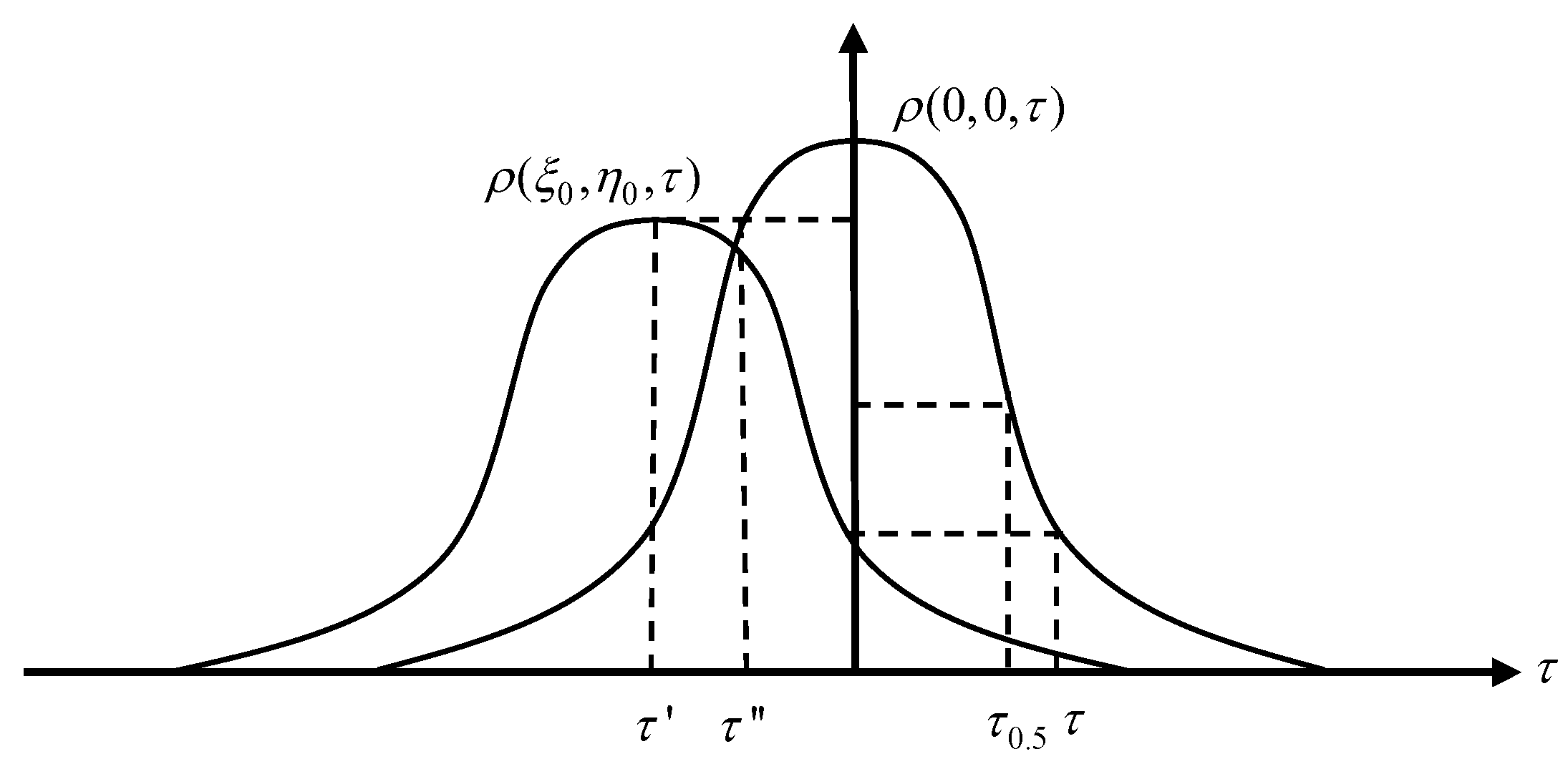
Suppose there is a set of antennas spaced apart by $({\xi }_0,{\eta }_0)$. According to Equation (1), the corresponding autocorrelation function is denoted by $\rho (0,0,\tau )$, and the cross-correlation function is denoted by $\rho ({\xi }_0,{\eta }_0,\tau )$, where $\rho (0,0,\tau )$ and $\rho ({\xi }_0,{\eta }_0,\tau )$ are collectively referred to as the correlation functions of this antenna array. Using these correlation functions, a set of correlation parameters, $\tau$, ${\tau }_{0.5}$, $\tau \prime$, and $\tau ″$, can be determined. Here, $\tau$ represents the time delay corresponding to when the autocorrelation function decreases to $\rho (0,0,\tau )$ and the cross-correlation function has a value of $\rho ({\xi }_0,{\eta }_0,\tau )$ at zero delay; ${\tau }_{0.5}$ represents the time delay corresponding to when the autocorrelation function $\rho (0,0,\tau )$ decreases to half of its peak value; $\tau \prime$ represents the time delay corresponding to the peak of the cross-correlation function $\rho ({\xi }_0,{\eta }_0,\tau )$; $\tau ″$ represents the time delay corresponding to when the autocorrelation function $\rho (0,0,\tau )$ increases to the same value as the cross-correlation function $\rho ({\xi }_0,{\eta }_0,\tau )$ at its peak. Specifically, as shown in Figure 1, using these correlation functions, the coefficients in Equation (2) can be determined.

Therefore, the key to the FCA method lies in determining the correlation functions. The calculation methods for the autocorrelation function and the cross-correlation function are as follows: assuming the received echo signal at antenna $\alpha =(x_i,y_i)$ is $f_{\alpha }(t)$, the autocorrelation function $f_{\alpha }(t)$ is defined as [14]:

$${\rho }_{\alpha }({\tau }_k)={\displaystyle \frac{[f_{\alpha }(t)f_{\alpha }^{\ast }(t+{\tau }_k)]}{[|f_{\alpha }(t){|}^2]}}$$

(3)

where the symbol $[·]$ denotes statistical averaging. By expanding the continuous signal into a time series and performing statistical averaging, the autocorrelation function can be expressed as:

$${\rho }_{\alpha }({\tau }_k)={\displaystyle \frac{{\displaystyle \sum _{n=1}^{N_r-|k|}{f}_{\alpha }(t)f_{\alpha }^{\ast }(t+{\tau }_k)}}{(N_r-|k|){\displaystyle \sum _{n=1}^{N_r}|f_{\alpha }(t){|}^2}}}$$

(4)

Similarly, assuming the received echo signals at antenna $\alpha =(x_i,y_i)$ are $f_{\alpha }(t)$, and the signals at antenna $b=(x_l,y_m)$ are $f_b(t)$, the cross-correlation function between $f_{\alpha }(t)$ and $f_b(t)$ is defined as:

$${\rho }_{\alpha b}({\tau }_k)={\displaystyle \frac{[f_{\alpha }(t)f_b^{\ast }(t+{\tau }_k)]}{\sqrt{[|f_{\alpha }(t){|}^2][|f_b(t){|}^2]}}}$$

(5)

The cross-correlation function, after statistical averaging and expansion, is expressed as:

$${\rho }_{\alpha b}({\tau }_k)={\displaystyle \frac{{\displaystyle \sum _{n=1}^{N_r-|k|}{f}_{\alpha }(t)f_b^{\ast }(t+{\tau }_k)}}{(N_r-|k|)\sqrt{{\displaystyle \sum _{n=1}^{N_r}|f_{\alpha }(t){|}^2}{\displaystyle \sum _{n=1}^{N_r}|f_b(t){|}^2}}}}$$

(6)

The accuracy of computing the correlation function directly determines the precision of the final calculated values. The influence of noise on the waveform of the correlation function can cause deviations in the computed correlation function from the true values. Below, we illustrate this with a simple numerical simulation.

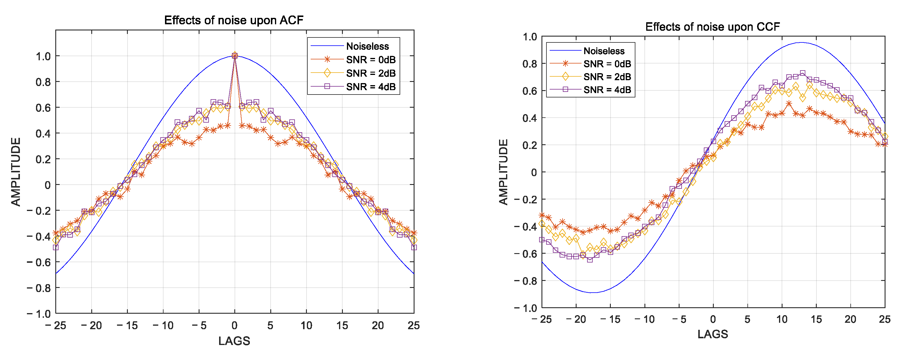
First, two sinusoidal sequences, $s(t)=\sin (t)$, $s\prime (t)=\sin (t+5)$, $(t=0,0.1,\dots ,20)$, each with 200 points, are generated. Then, additive Gaussian white noise with a signal-to-noise ratio (SNR) of 0 dB, 2 dB, and 4 dB is added to $s(t)$ and $s\prime (t)$ to generate noisy sinusoidal sequences, $s_n(t)$ and $s_n\prime (t)$. Using Equation (4), the amplitudes of the autocorrelation functions of $s_n(t)$ at different SNRs are calculated, as shown in the left graph of Figure 2. Similarly, using Equation (5), the amplitudes of the cross-correlation functions between $s_n(t)$ and $s\prime (t)$ at different SNRs are calculated, as shown in the right graph of Figure 2.

From Figure 1 and Figure 2, it can be observed that noise significantly impacts the amplitudes of both types of correlation functions, the autocorrelation function and the cross-correlation function, within the main lobe range. The amplitudes decrease and exhibit distortion as the SNR decreases. This distortion in the correlation functions can introduce errors in the FCA retrieval process. David’s theory addresses this issue by correcting the amplitudes of the correlation functions to determine the attenuation coefficient, referred to as the noise factor. This noise factor aims to minimize the deviation of the autocorrelation function values under noisy conditions from those under noise-free conditions [24].

Assuming antenna ${\alpha }_i$ receives an echo signal composed of both the signal $s_i(t)$ and noise $n_i(t)$, the received signal can be represented as $f_i(t)$:

$$f_i(t)=s_i(t)+n_i(t)$$

(7)

Since the signal and noise are uncorrelated, their statistical mean is zero [14]. Where $[s_i(t)n_j({\tau }_k)]=0 \forall i,j,k$.

Based on specific statistical characteristics, noise can be further categorized into two types, correlated noise and uncorrelated noise, as follows:

(1) Noise that has certain correlations between different antennas due to coupling after reception $n_{ci}(t)$, where $[n_{ci}{n}_{ci}^{\ast }]\ne 0 i\ne j$.

This type of noise includes atmospheric background noise, power supply noise, and artificial noise, among others.

(2) This type of noise, which includes receiver noise and galactic background noise, lacks correlation noise $n_{ui}(t)$ between different antennas after reception. The subdivided noise can be expressed as $n_i(t)=n_{ci}(t)+n_{ui}(t)$.

According to the definitions of $n_{ci}(t)$ and $n_{ui}(t)$, and utilizing their respective statistical properties, the following statistical laws can be derived, where $i=j$ represents the same antenna:

$$\begin{array}{l}[n_i(t)n_j^{\ast }(t+{\tau }_k)]=0 {\tau }_k\ne 0 \mathrm{or} {\tau }_k=0 \mathrm{and} i\ne j\\ [n_{ci}(t)n_{ci}^{\ast }(t+\tau )]=0 {\tau }_k\ne 0\\ [n_{ci}(t)n_{ui}^{\ast }(t+{\tau }_k)]=0 \forall i,j,{\tau }_k\\ [n_{ci}(t)n_{ui}^{\ast }(t+{\tau }_k)]=0 {\tau }_k\ne 0 \mathrm{or} {\tau }_k=0 \mathrm{and} i\ne j\end{array}$$

(8)

Utilizing these statistical laws of noise, we can further derive the expanded forms of the autocorrelation and cross-correlation functions.

Since any signal is correlated with itself, expanding $f_i(t)$ in Equation (7) as a combination of signal and noise, the autocorrelation function can be rewritten as Equation (9) (where ${\tau }_k$ is abbreviated for noise $\tau$).

$$\rho (\tau )={\displaystyle \frac{[(s_i(t)+n_i(t)){(s_i(t+\tau )+n_i(t+\tau ))}^{\ast }]}{[|s_i(t)+n_i(t){|}^2]}}$$

(9)

Expanding the autocorrelation function yields:

$$\rho (\tau )=\left\{\begin{array}{l}1,\tau =0\\ {\displaystyle \frac{[(s_i(t)+n_i(t)){(s_i(t+\tau )+n_i(t+\tau ))}^{\ast }]}{[|s_i(t)+n_i(t){|}^2]}},\tau \ne 0\end{array}\right.$$

(10)

Comparing Equations (4) and (17), when $\tau \ne 0$.

$$\rho (\tau )={\displaystyle \frac{[|s_i(t){|}^2]}{[|s_i(t){|}^2]+[|n_i(t){|}^2]}}\ast {\displaystyle \frac{[s_i(t)s_i(t+\tau )]}{[|s_i(t){|}^2]}}={\displaystyle \frac{[|s_i(t){|}^2]}{[|s_i(t){|}^2]+[|n_i(t){|}^2]}}\ast {\rho }_i({\tau }_k)$$

(11)

We define:

$$F_i={\displaystyle \frac{[|s_i(t){|}^2]+[|n_i(t){|}^2]}{[|s_i(t){|}^2]}}$$

(12)

Here, $F_i$ is called the noise factor of $s_i(t)$. Multiplying all non-zero values of the expression for the autocorrelation function under noise in Equation (11) by $F_i$ yields the estimate of the autocorrelation function without noise:

$$\rho (\tau )=\left\{\begin{array}{l}1,\tau =0\\ {\displaystyle \frac{{\rho }_i({\tau }_k)}{F_i}},\tau \ne 0\end{array}\right.$$

(13)

The value of the autocorrelation function at zero delay must be 1. As $\tau$ approaches 0, the autocorrelation function under noise tends towards $1/F_i$, so $F_i$ can be determined from this.

Similarly, the cross-correlation function $f_i(t)$ and $f_j(t)$ in Equation (6), when expanded as a combination of signal and noise, can be rewritten as:

$${\rho }_{ij}(\tau )={\displaystyle \frac{[(s_i(t)+n_i(t)){(s_j(t+\tau )+n_j(t+\tau ))}^{\ast }]}{\sqrt{[|s_i(t)+n_i(t){|}^2][|s_j(t)+n_j(t){|}^2]}}}$$

(14)

Finally, the cross-correlation function can be expressed as:

$${\rho }_{ij}(\tau )=\left\{\begin{array}{l}{\displaystyle \frac{[s_j(t)s_j^{\ast }(t)]+[n_i(t)n_j^{\ast }(t)]}{\sqrt{\left([|s_i(t){|}^2]+[|n_i(t){|}^2]\right)\left([|s_j(t){|}^2]+[|n_j(t){|}^2]\right)}}},\tau =0\\ {\displaystyle \frac{s_i(t)s_j^{\ast }(t+\tau )}{\sqrt{\left([|s_i(t){|}^2]+[|n_i(t){|}^2]\right)\left([|s_j(t){|}^2]+[|n_j(t){|}^2]\right)}}},\tau \ne 0\end{array}\right.$$

(15)

Analyzing Equation (15), when $\tau \ne 0$.

$$\begin{array}{l}{\rho }_{ij}(\tau )={\displaystyle \frac{s_i(t)s_j^{\ast }(t+\tau )}{\sqrt{\left([|s_i(t){|}^2]+[|n_i(t){|}^2]\right)\left([|s_j(t){|}^2]+[|n_j(t){|}^2]\right)}}}\\ ={\displaystyle \frac{\sqrt{\left([|s_i(t){|}^2]\right)}}{\sqrt{\left([|s_i(t){|}^2]+[|n_i(t){|}^2]\right)}}}\ast {\displaystyle \frac{\sqrt{[|s_j(t){|}^2]}}{\sqrt{\left([|s_j(t){|}^2]+[|n_j(t){|}^2]\right)}}}\ast {\displaystyle \frac{s_i(t)s_j^{\ast }(t+\tau )}{\sqrt{[|s_i(t){|}^2]\ast [|s_j(t){|}^2]}}}\end{array}$$

(16)

According to the definition of the noise factor in Equation (13), Equation (15) can be rewritten as:

$${\rho }_{ij}(\tau )={\displaystyle \frac{s_i(t)s_j^{\ast }(t+\tau )}{\sqrt{F_i{F}_j}\ast \sqrt{[|s_i(t){|}^2]\ast [|s_j(t){|}^2]}}}={\displaystyle \frac{{\rho }_{ab}(\tau )}{\sqrt{F_i{F}_j}}}$$

(17)

If $F_i{F}_j$ is known, radar parameters ${\rho }_{ij}(0)$ can be calculated at $\tau =0$ using Equation (17). Here, is the noise factor $s_i(t)$ for antenna $F_i$, and is the noise factor $s_j(t)$ for antenna $F_j$, with each noise factor originating from the noise of the signals received by the respective antennas.

The key to estimating the autocorrelation and cross-correlation functions lies in computing the noise factor. The definitions and computational formulas for the correlation functions are presented in

Table 1. The definitions and calculation formulas of the correlation functions, the influence of noise on the correlation functions, and the corresponding noise reduction methods.

	Autocorrelation Function	Cross-Correlation Function
Definition without noise	${\rho }_{\alpha }({\tau }_k)={\displaystyle \frac{[f_{\alpha }(t)f_{\alpha }^{\ast }(t+{\tau }_k)]}{[|f_{\alpha }(t){|}^2]}}$	${\rho }_{\alpha b}({\tau }_k)={\displaystyle \frac{[f_{\alpha }(t)f_b^{\ast }(t+{\tau }_k)]}{\sqrt{[|f_{\alpha }(t){|}^2][|f_b(t){|}^2]}}}$
Calculation without noise	${\rho }_{\alpha }({\tau }_k)={\displaystyle \frac{{\displaystyle \sum _{n=1}^{N_r-|k|}{f}_{\alpha }}(t)f_{\alpha }^{\ast }(t+{\tau }_k)}{(N_r-|k|){\displaystyle \sum _{n=1}^{N_r}|f_{\alpha }(t){|}^2}}}$	${\rho }_{\alpha b}({\tau }_k)={\displaystyle \frac{{\displaystyle \sum _{n=1}^{N_r-|k|}{f}_{\alpha }}(t)f_b^{\ast }(t+{\tau }_k)}{\sqrt{{\displaystyle \sum _{n=1}^{N_r}|f_{\alpha }(t){|}^2}{\displaystyle \sum _{n=1}^{N_r}|f_b(t){|}^2}}}}$
With noise	$\rho (\tau )=\left\{\begin{array}{cc}1& ,\tau =0\\ {\displaystyle \frac{[s_i(t)s_i^{\ast }(t+\tau )]}{[|s_i(t){|}^2]+[|n_i(t){|}^2]}},& \tau \ne 0\end{array}\right.$	${\rho }_{ij}(\tau )=\left\{\begin{array}{l}{\displaystyle \frac{[s_j(t)s_j^{\ast }(t)]+[n_{ci}(t)n_{cj}^{\ast }(t+\tau )]}{\sqrt{([|s_i(t){|}^2]+[|n_i(t){|}^2])([|s_j(t){|}^2]+[|n_j(t){|}^2])}}},(\tau =0)\hfill \\ {\displaystyle \frac{s_i(t)s_j^{\ast }(t)}{\sqrt{([|s_i(t){|}^2]+[|n_i(t){|}^2])([|s_j(t){|}^2]+[|n_j(t){|}^2])}}},(\tau \ne 0)\hfill \end{array}\right.$
Noise reduction	$\begin{array}{l}{\rho }^{\prime }(\tau )=\rho (\tau )F_i={\displaystyle \frac{[s(t)s_i^{\ast }(t+{\tau }_k)]}{[|s(t){|}^2]}}\\ F_i={\displaystyle \frac{[|s_i(t){|}^2]+[|n_i(t){|}^2]}{[|s_i(t){|}^2]}}\end{array}$	$\begin{array}{l}{\rho }_{ij}^{\prime }(\tau )={\rho }_{ij}(\tau )\sqrt{F_i{F}_j}={\displaystyle \frac{[s_i(t)s_j^{\ast }(t+{\tau }_k)]}{\sqrt{[|s_i(t){|}^2][|s_j(t){|}^2]}}}\\ \sqrt{F_i{F}_j}=\sqrt{{\displaystyle \frac{[|s_i(t){|}^2]+[|n_i(t){|}^2]}{[|s_i(t){|}^2]}}}\sqrt{{\displaystyle \frac{[|s_j(t){|}^2]+[|n_j(t){|}^2]}{[|s_j(t){|}^2]}}}\end{array}$

.

3. Correction Steps for the Amplitude of Correlation Functions

The autocorrelation function curve can be fitted using an even-degree polynomial to determine the noise factor. Assuming the signal to be tested is a standard sine wave $y(x)=\alpha \sin ({\omega }_{0}x+\varphi )$, for simplicity, the sampling frequency of x is denoted as $f$, $\omega ={\omega }_0\ast f$, and $y(m)=\alpha \sin (\omega m+\varphi )$, where m is an integer. If the measurement time T is long enough, the expression for its autocorrelation function is:

$$R_{xx}(k)={\displaystyle \frac{1}{T}}{\displaystyle \underset{0}{\overset{T}{\int }}\alpha \sin (\omega m+\varphi )}\ast \alpha \sin [\omega (m+k)+\varphi ]dx={\displaystyle \frac{{\alpha }^2}{2}}\cos (\omega k)$$

(18)

To avoid interference from the coefficient values $\alpha$, the autocorrelation value at $\tau =0$ can be normalized, yielding $\rho (k)=\cos (\omega k)$.

Similarly, if the signal under test is the superposition of n sine waves (this is a commonly used assumption for narrow band signals as per [28]), $y(x)={\displaystyle \sum _{i=1}^n{\alpha }_i\sin ({\omega }_{oi}x+{\varphi }_i)}$, where $f$ is the sampling frequency of x, ${\omega }_i={\omega }_{oi}\ast f$, so that $y(m)={\displaystyle \sum _{i=1}^n{\alpha }_i\sin ({\omega }_{i}m+{\varphi }_i)}$, m is an integer. If the measurement time T is long enough, its autocorrelation function expression is as follows:

$$R_{xx}(k)={\displaystyle \frac{1}{T}}{\displaystyle \underset{0}{\overset{T}{\int }}y(m)\ast y(m+k)dx}={\displaystyle \sum _{i=1}^n\frac{{\alpha }_i^2}{2}\cos ({\omega }_{i}k)}$$

(19)

After normalization, the expression becomes as follows:

$$\rho (k)={\displaystyle \frac{{\displaystyle \sum _{i=1}^n\frac{{\alpha }_i^2}{2}\cos ({\omega }_{i}k)}}{{\displaystyle \sum _{i=1}^n\frac{{\alpha }_i^2}{2}}}}$$

(20)

From the results, it is observed that:

(1) When n is a finite integer value, the expression for $\rho (k)$ is a sum of finite cosine functions. Using the Taylor series expansion of cosine functions, it can be determined that there exists a unique constant array C satisfying:

$$\rho (k)=c_0+c_2{x}^2+c_4{x}^4+o(x^4)$$

(21)

Then, based on Equation (14), $F_i$ can be estimated using a fitting method. From Equations (20) and (21), it can be seen that the fitting function can be selected from the following three functions: $\alpha \cos (bx)$, $c_1{x}^2$, $c_1{x}^2+c_2{x}^4$ (cosine fitting, quadratic fitting, and quartic fitting). In the fitting process, the fitting points are evenly distributed around $\tau =0$ but do not include the point 0.

(2) The cosine functions $\rho (k)$ in Equation (20) have periods related to the angular frequency of the original signal and the sampling frequency. Therefore, the accuracy of the fitting results can be improved by suppressing noise through an appropriate choice of sampling frequency. In cosine fitting, if the angular frequencies of the parameters in $\rho (k)$ are known, the fitting process can be simplified. Otherwise, it is necessary to estimate the angular frequencies of each component, complicating the fitting function and making the process more time-consuming. However, radar data typically involve a large amount of data, and complex fitting calculations are not suitable for real-time radar data processing.

Taking two 200-point sine wave sequences $s(t)=\sin (t)$ and $s\prime (t)=\sin (t+5)$$(t=0,0.1,\dots ,20)$ as an example, additive Gaussian white noise with SNRs of 0 dB, 2 dB, and 4 dB is added to $s(t)$ and $s\prime (t)$ to generate noisy sine wave sequences $s_n(t)$ and $s_n\prime (t)$.

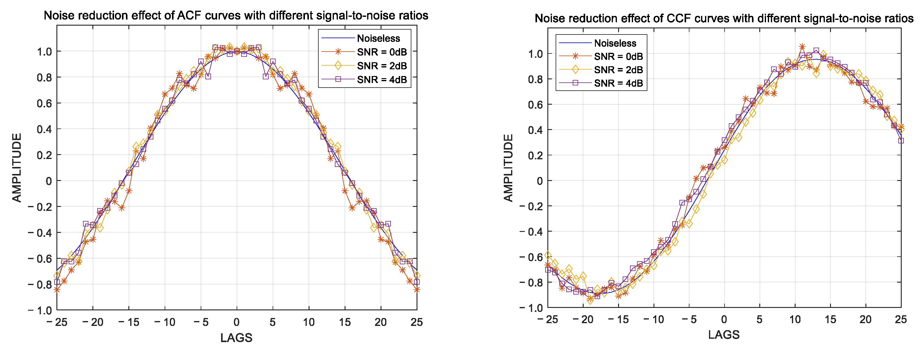
The autocorrelation functions, obtained after adding additive Gaussian white noise, are then fitted with a second-order polynomial using 10 points around the zero-delay point to calculate the noise factor. Finally, the curves of the autocorrelation and cross-correlation functions in Figure 2 are denoised and corrected, as shown in Figure 3.

Comparing Figure 2 with Figure 3, it is observed that the noise factor fitted by the polynomial significantly corrects the amplitude of the autocorrelation function. According to the definition of SNR, an estimation of its value can be made.

Regarding the application analysis of fitting methods, although the radar can receive thousands of raw data points per second, it requires hundreds of original data to calculate a single data point. Therefore, in this study of $\cos (2\mathsf{\pi }fk)$, the range of $f$ is generally from $2<f<10$ corresponding to a large SNR error. However, for the FCA method, the academic community is more concerned with the calculation of the autocorrelation function. The amplitude correction of the distorted correlation function is performed using the proposed polynomial fitting-based noise reduction (PFNR) method, as shown in Algorithm 1.

Algorithm 1. PFNR Algorithm

Input: Receive signal; sampling frequency; fitting order Output: Correlation function amplitude correction

1. Calculate correlation function.  According to Equations (4) and (6) to calculate correlation function. 2. Polynomial fitting.  2.1 Remove the point where the autocorrelation function is at 0 lags.  2.2 Set an appropriate fitting order.  2.3 Take an appropriate number signal data points around 0 lags for fitting.  2.4 Use fitting to obtain the value of autocorrelation function at 0 lags. 3. Calculate the noise factor $F_i$.  According to Equations (11) and (12) to calculate $F_i$. 4. Correct the amplitude of the correlation function.  Multiply $F_i$ by autocorrelation function without the value of 0 lags to obtain amplitude correction.

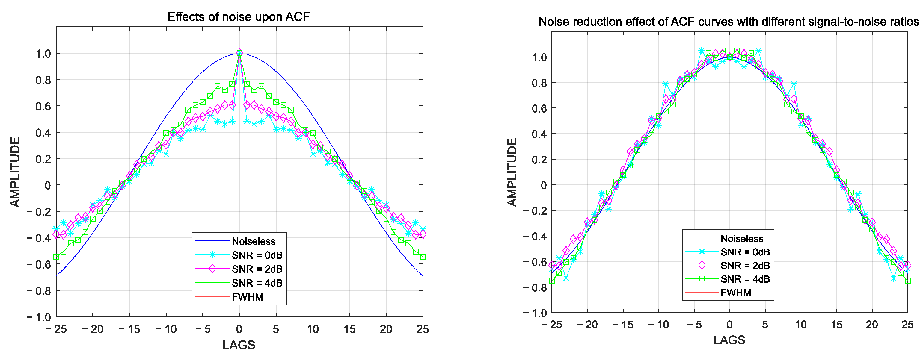
Taking ${\tau }_{0.5}$ as an example, its equivalent point is the delay point corresponding to the half-wave width point of the autocorrelation function curve. Figure 4 illustrates the comparison results between the original autocorrelation function (left) and the autocorrelation function after noise reduction using the quadraticfitting method (right).

It can be observed that, although, theoretically, fitting methods result in larger errors in low-frequency sampled signals, they still exhibit significant effectiveness in estimating the radar autocorrelation function. Moreover, these methods are straightforward and do not significantly increase radar data processing time, making them suitable for practical applications. In the application of the proposed PFNR algorithm, the fitting function’s order n and frequency can influence fitting performance, and hence the estimation performance of ${\tau }_{0.5}$. In the following section, we will investigate this problem.

4. Performance of the PFNR Algorithm

To evaluate the performance of various methods for estimating atmospheric wind speed, certain quantitative indicators are necessary. The Mean Squared Error (MSE) measures the difference between an estimated value and an actual value. It calculates the average of the squares of the differences between the estimated and actual values, which can be used to evaluate the prediction accuracy of the model. The smaller the MSE, the higher the accuracy of the model’s predictions. Therefore, MSE is used to evaluate performance. Currently, existing methods for estimating wind speed include direct estimation and indirect estimation through relevant parameters [21,22]. In the process of the proposed PFNR algorithm, $F_i$, or, equivalently, $\widehat{\rho }(k|k=0)$, is a byproduct in the estimation of delay parameters and hence the wind speed. We find that:

$$\begin{array}{l}{\mathrm{SNR}}_{estimate}\\ =10{\log }_{10}\left({\displaystyle \frac{[|s_i(t){|}^2]}{[|n_i(t){|}^2]}}\right)\\ =10{\log }_{10}\left({\displaystyle \frac{[|s_i(t){|}^2]}{[|s_i(t){|}^2]+[|n_i(t){|}^2]}}\ast {\displaystyle \frac{[|s_i(t){|}^2]+[|n_i(t){|}^2]}{[|n_i(t){|}^2]}}\right)\\ =10{\log }_{10}\left({\displaystyle \frac{\widehat{\rho }(k|k=0)}{1-\widehat{\rho }(k|k=0)}}\right)\end{array}$$

(22)

in which, $\widehat{\rho }(k|k=0)$ indicates that it is an estimated value using the polynomial fitting method according to the proposed PFNR algorithm. Thus, the value of $SN{R}_{estimate}$ can be a measure of the proposed PFNR algorithm. Using Equation (22), the estimated value of SNR can be calculated from the value at the zero-delay point of the autocorrelation function $\widehat{\rho }(k|k=0)$. The difference between the estimated $SN{R}_{estimate}$ and the true value $SN{R}_{true}$ is $SN{R}_{error}=SN{R}_{estimate}-$$SN{R}_{true}$, and it can serve as a metric to evaluate the performance of the noise reduction process. The closer the estimation error $SN{R}_{error}$ is to zero, the better the performance of the noise reduction. In this work, the polynomial fitting method is used to correct the amplitude of the correlation function and evaluate it by the MSE of SNR. The factors affecting the evaluation mainly include the order of fitting and the sampling frequency. These two influencing factors are analyzed in the following sections.

For a fair comparison, the range of data used is fixed from −20 to 20 lags. Simulations are conducted for two cases of additive white noise signals:

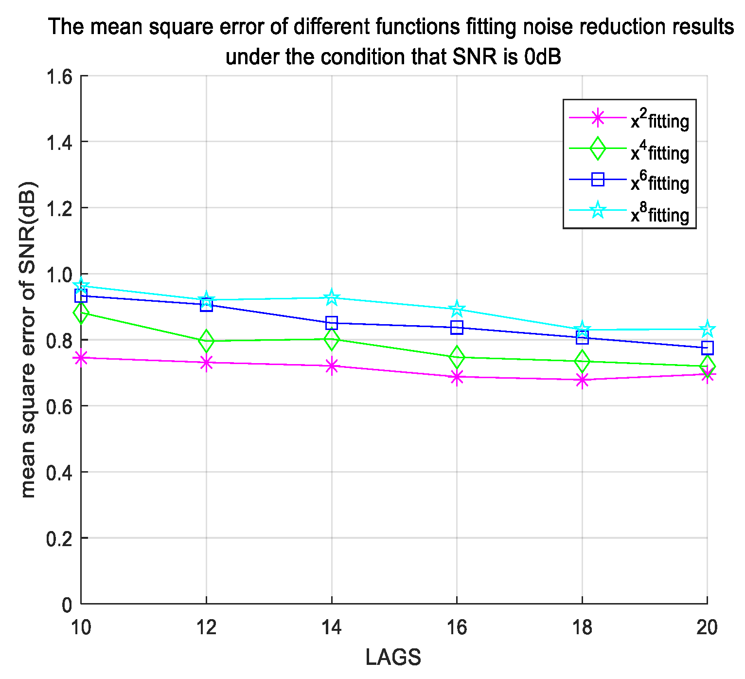
(1) First, a sinusoidal sequence $s(t)=\sin (t)$ $(t=0,0.1,\dots ,20)$ is generated. Gaussian white noise with a SNR of 0 dB is added to $s(t)$. Finally, based on Equation (22), the mean square value of the error data for 10,000 cases of $s_n(t)$ under SNR of 0 dB is calculated as the number of fitting points increases. Figure 5 corresponds to $s(t)$. From Figure 5, it can be observed that, under the same conditions, the $SN{R}_{estimate}$ obtained by the quadratic fitting is the lowest. Simultaneously,

Table 2. The fitting time complexity of various fitting methods with the number of fitting points of 10.

Fitting Methods	Runtime (s)
$x^2$ fitting	0.000019
$x^4$ fitting	0.000021
$x^6$ fitting	0.000023
$x^8$ fitting	0.000026

presents the fitting time complexity of different methods under the same conditions and a fitting point of 10, indicating that the quadratic fitting exhibits the lowest time complexity.

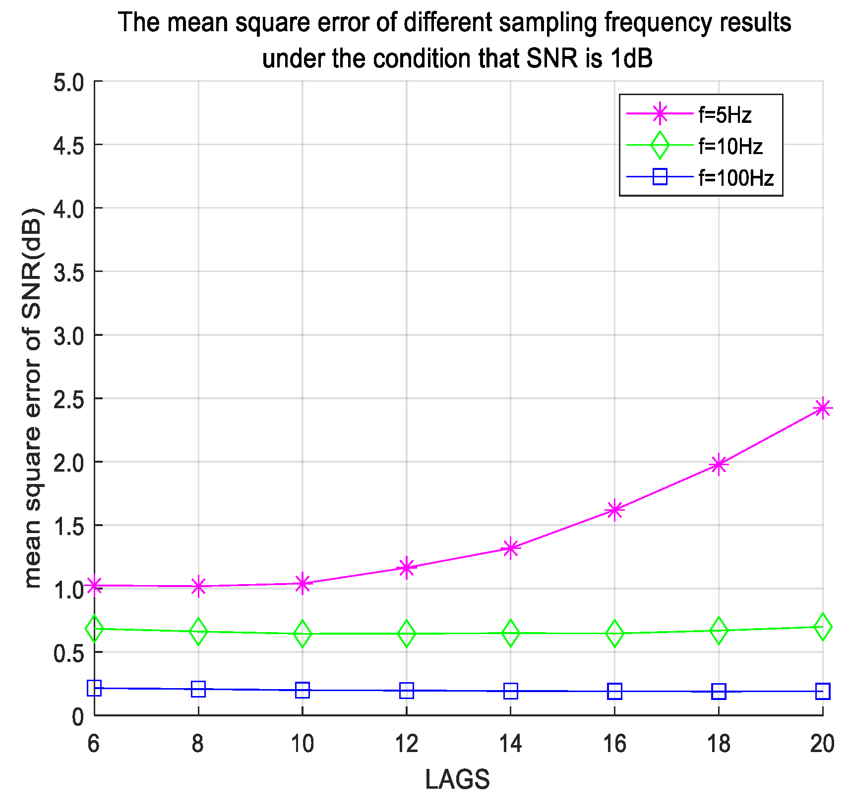
(2) To better simulate real-world scenarios, the signal $y=\sin (2x+5)+2\sin (x)$ $(t=0,0.1,\dots ,20)$ is chosen. In view of the results of simulation (1), quadratic fittings are adopted, and MSE is calculated, as shown in Figure 6. From Figure 6, it is observed that, under the same conditions, the range of MSE decreases with the increase in sampling frequency. This is mainly attributed to the cosine factor $\cos (2\mathsf{\pi }fk)$ in the theoretical expression of the autocorrelation function $\widehat{\rho }(k)$, which becomes finer “interpolation” for $\cos (k)$ with increasing sampling frequency, thus better suppressing noise. According to the simulation results, when $f=5$, the minimum value of MSE is around 1 (Figure 6); when $f=10$, the minimum value of MSE is around 0.7; and when $f=100$, the minimum value of MSE is around 0.2. Since the error curve of quadratic fitting approximates a parabola, quadratic fitting should be preferred when the sampling frequency is low. Otherwise, when fitting with more points, quartic fitting should be preferred.

5. Conclusions

This work proposes an amplitude correction method for the noise factor of sinusoidal sequences using the correlation function, which can be applied to data processing of the autocorrelation and cross-correlation functions of MF Radar. The MSE of noise reduction with different fitting methods is analyzed as the number of fitting points changes. In the scenario set in this study, since the error curve of quadratic fitting approximates a parabola, quadratic fitting performs better than other fitting methods. For a deeper analysis, the impact of different sampling frequencies on polynomial fitting is further examined through numerical simulation under the same SNR. Simulation results indicate that a higher data sampling frequency leads to better amplitude correction of the correlation function, while a smaller number of fitting points is suitable for quadratic fitting.