Sensitivity Analysis of the Inverse Distance Weighting and Bicubic Spline Smoothing Models for MERRA-2 Reanalysis PM_2.5 Series in the Persian Gulf Region

Abstract

Various studies have proved that PM_2.5 pollution significantly impacts people’s health and the environment. Reliable models on pollutant levels and trends are essential for policy-makers to decide on pollution reduction. Therefore, this research presents the sensitivity analysis of the Bicubic Spline Smoothing (BSS) and Inverse Distance Weighting (IDW) models built for the PM_2.5 monthly series from MERRA-2 Reanalysis collected during January 2010–April 2017 in the region of the Persian Gulf, in the neighborhood of the United Arab Emirates Coast. The models’ performances are assessed using the Mean Absolute Error (MAE), Root Mean Square Error (RMSE), and Mean Absolute Percentage Error (MAPE). RMSE, Mean Bias Error (MBE), and Nash–Sutcliff Efficiency (NSE) were utilized to assess the models’ sensitivity to various parameters. For the IDW, the Mean RMSE decreases as the power parameter increases from 1 to approximately 4 (the optimal beta value) and then stabilizes with a further increase. NSE values close to 1 indicate that the model’s predictions are very efficient in capturing the variance of the observed data. NSE is almost constant as a function of the number of neighbors and the parameter when β > 4. In BSS, the RMSE and NBE plots suggest that incorporating more points into the mean calculation for buffer points leads to a general decrease in model accuracy. Moreover, the MBE plot shows that the mean bias error initially increases with the number of points but then starts to plateau. The increasing trend suggests that the model tends to systematically overestimate the PM_2.5 values as more points are included. The leveling-off of the curve indicates that beyond a certain number of points, the bias introduced by including additional points does not significantly increase, suggesting a threshold beyond which further inclusion of points does not markedly change the mean bias. It was also proved that the methods’ generalizability may depend on the dataset’s specific spatial characteristics.

1. Introduction

Pollution, a significant threat in the post-industrial era, necessitates our immediate attention. Observing, modeling, and predicting its evolution are crucial steps in making urgent decisions to reduce and, if possible, eliminate the sources [1,2,3,4].

PM_2.5—fine particulate matter with diameters smaller than 2.5 μm—is a composition of particles found in the atmosphere in a solid or liquid state [5]. These particles, originating from natural processes such as forest fires, volcanic eruptions, dust storms, and anthropic activities like wood or fossil fuel combustion [6,7,8], can persist in the atmosphere due to their physical and chemical properties, coupled with meteorological conditions, leading to pollution [9,10,11]. Their minuscule size makes them easily inhalable and prone to deposition on various parts of the respiratory system, causing a range of diseases and even premature deaths [5,12,13].

The international reports reveal a shocking reality about the United Arab Emirates (UAE): the average annual concentration of PM_2.5 was eight times higher than the upper limits (5 μg/m³) imposed by the WHO for the population exposure to these pollutants. According to recent studies, sandstorms are not the main contributors to the decreasing quality of the air in the UAE, but the industry (mainly the fossil fuels emissions), followed by road transportation [14,15,16,17].

Moreover, from 2000 to 2019, the UEA’s exposure to PM_2.5 was more than 2.3 times higher than in all the European Union or OECD countries [18].

Given the urgent need to mitigate the effects of PM_2.5 and PM₁₀ on public health, different solutions for purifying indoor air have also been proposed [19,20]. Many scientific studies are dedicated to monitoring and estimating the concentration of particulate matter, considering the atmospheric conditions [21].

However, the current density of monitoring networks is insufficient, necessitating interpolation methods to assess pollutant concentrations in areas without available records. Particulate matter concentrations can vary rapidly at the same site or between different locations, so it is vital to have accurate modeling tools that require a reasonable number of observation points and records.

Many methods have been employed to achieve reliable modeling of spatially distributed data series. Some examples are provided in the following. Li et al. [22] utilized IDW for interpolating the PM_2.5 series in the United States, whereas Choi and Chong [23] proposed a new version of IDW applied for series from South Korea and proved its increased performance against the classical IDW and kriging [24]. Diggle and Ribeiro [25] proposed model-based geostatistics. A comparison of different geostatistical methods for evaluating exposure to PM_2.5 was presented by Lee et al. [26]. Spatial interpolation and spatio-temporal interpolation of large data series are presented [27,28,29,30,31].

Other approaches involve the use of Artificial Intelligence (AI), including Machine Learning (ML) and Deep Learning DL) Techniques. Artificial neural networks (Multilayer Perceptron, Long-short-term memory, Convolutional Neural Networks) were built by Goudarzi et al. [32], Ma et al. [33], Xiao et al. [34], Chae et al. [35], and to describe the PM series evolution. Rizos et al. [36] proposed an ML model to characterize the PM₁₀ background pollution in a region of Greece. The Air Pollution Model (TAPM) for real-time weather forecast and the PM₁₀ daily average concentration is presented by Zoras et al. [37]. Other valuable methods for the particulate matter series modeling and forecast are exponential smoothing [38], ensemble methods [39], remote sensing [40], or hybrid techniques [41,42,43,44]. Each tackles specific challenges to enhance the models’ performance, which is critical for using the modeling results in the prediction.

The literature search shows that most articles on the spatial interpolation of the PM_2.5 concentration series do not provide a sensitivity analysis of the models despite this aspect being essential for assessing the method’s generalizability, efficacy, and stability, especially when it involves the selection of various parameters (that must be optimized) or the ratio training/test sets (in the artificial intelligence methods).

Our findings have significant practical implications because the model most insensitive to the variation in parameters is the most efficient when dealing with different databases. This insight can guide future research and application of spatial interpolation models, in particular for pollutants’ concentration series. Therefore, in this article, we present the sensitivity analysis of the Bicubic Spline Smoothing and Inverse Distance Weighting (IDW) models built for the PM_2.5 average monthly series (μg/m³) from MERRA-2 Reanalysis from the region of Persian Gulf, in the neighborhood of the United Arab Emirates Coast. The models’ performance is assessed using multiple indicators, and the best choice is emphasized. It is shown that the IDW performances are similar after a particular value of the beta parameter. In BSS, increasing the sample involved in the computation for buffer points above an estimated level decreases the model accuracy.

2. Materials and Methods

2.1. Data Series

The monthly data set covering January 2010–April 2017 was downloaded from the tavgM_2d_aer_Nx 2-dimensional data collection in Modern-Era Retrospective analysis for Research and Applications version 2 (MERRA-2) [45]. Figure 1 presents the grid points’ location and coordinates, and Figure 2 represents the data series from sites 60–70.

MERRA-2 is NASA’s Global Modeling and Assimilation Office’s newest analysis of the Earth’s atmosphere using satellite data. It includes new types of observations and updates to the GEOS model and analysis method [46].

Reanalysis, a process involving the consistent reprocessing of meteorological records by an unchanging data assimilation system, is a reliable method that usually covers a long period. It relies on a forecast model to merge different observations in a physically coherent way, enabling the creation of gridded data sets for various variables, including those that are indirectly observed or sparse [46].

The PM_2.5 concentrations varied between 14.30 and 246.00 $\mathsf{\mu }$g/m³, with an average between 36.49 and 119.36 $\mathsf{\mu }$g/m³ and standard deviations in the interval 13.19–37.34 $\mathsf{\mu }$g/m³. Most variations are due to the seasonality and the position of the point in the grid (over the sea or the continent).

2.2. Modeling

As we delve into the sensitivity analysis, it is worth noting that the modeling stage has been comprehensively detailed in [30]. In this article, we will briefly outline the methodology used to derive the models, focusing on the new aspect–sensitivity analysis.

The first interpolation approach for the data series was the IDW [47].

Given the set $\left\{{(\mathit{x}}_{\mathit{k}}\right.$,${\mathit{z}}_{\mathit{k}}):{\mathit{x}}_{\mathit{k}}\in {\mathit{R}}^{\mathit{n}},{\mathit{z}}_{\mathit{k}}\in \left.\mathit{R}\right\}$, k = 1,…, m, the interpolation function is defined by the following:

$$\mathit{z}\left(\mathit{x}\right):{\mathit{R}}^{\mathit{n}}\to \mathit{R},$$

$$\widehat{z}\left(\mathit{x}\right)=\left\{\begin{array}{c}\left({\displaystyle \sum _{k=1}^m}\frac{{\mathit{z}}_{\mathit{k}}}{d_k^{\mathrm{\beta }}}\right)/\left({\displaystyle \sum _{k=1}^m}\frac{1}{d_k^{\mathrm{\beta }}}\right), if d_k\ne 0 for all k \\ {\mathit{z}}_{\mathit{k}},if d_k=0 for some k \end{array}\right.$$

(1)

where

$\widehat{z}\left(\mathit{x}\right) ({\mathit{z}}_{\mathit{k}}$)—the value estimated (recorded) at the point $\mathit{x}$ ${\left(\right(\mathit{x}}_{\mathit{k}}\left)\right)$;

$d_k$—distance between the points $\mathit{x}$ and ${\mathit{x}}_{\mathit{k}}$;

β > 1—parameter to be optimized (in the classical case, β = 2).

The second one was the Bicubic Spline Smoothing (BSS) [48] for interpolating 2-dimensional surfaces, defined by piecewise polynomial functions. In each cell of the grid (supposed to be rectangular), the interpolating function, with the coefficients ${\mathit{a}}_{\mathit{i}\mathit{k}}$ and variables x and y, is defined by:

$$P\left(x,y\right)=\sum _{i=0}^3\sum _{k=0}^3{a}_{ik}{x}^i{y}^k.$$

(2)

For a grid cell, to determine the coefficients $a_{ik}$, a system of 16 equations must be solved. The first four result from replacing the left-hand side of (2) with the values of the function in the grid corners. Using the derivatives

$${\partial }_{x}P\left(x,y\right)=\sum _{i=1}^3\sum _{k=0}^{3}i{a}_{ik}{x}^{i-1}{y}^k$$

(3)

$${\partial }_{y}P\left(x,y\right)=\sum _{i=0}^3\sum _{k=1}^{3}ik{x}^i{y}^{k-1}$$

(4)

$${\partial }_{xy}P\left(x,y\right)=\sum _{i=1}^3\sum _{k=1}^{3}ik{a}_{ik}{x}^{i-1}{y}^{k-1}$$

(5)

and the approximations

$${\partial }_{x}P\left(x,y\right)=\left[f\left(x+1,y\right)-f\left(x-1,y\right)\right]/2$$

(6)

$${\partial }_{y}P\left(x,y\right)=\left[f\left(x,y+1\right)-f\left(x,y-1\right)\right]/2$$

(7)

$${\partial }_{xy}P\left(x,y\right)=\left[f\left(x+1,y+1\right)-f\left(x-1,y\right)-\left(x,y-1\right)+f(x,y\right]/2,$$

(8)

we obtain the other 12 equations [49].

To address the issue of the boundary points having insufficient neighbors, we created a boundary buffer formed by artificially generated points around the grid’s perimeter. The values associated with the buffer are computed from the nearest neighbors’ means, which results in a smooth gradient aligning the original series distribution [30].

The error metrics used to compare different models were MAE, RMSE, MAPE, Nash–Sutcliffe Efficiency (NSE), Kling–Gupta Efficiency (KGE), and dIndex.

The last three indices are defined by:

$$NSE=1-\frac{{\sum }_{i=1}^m{(y_{obs,i}-y_{sim,i})}^2}{{\sum }_{i=1}^N{(y_{obs,i}-{\overline{y}}_{obs})}^2}$$

(9)

where m = the sample volume, $y_{obs,i}$ = the recorded value, $y_{sim,i}$ = the computed value, ${\overline{y}}_{obs}$ = average of the recorded values.

$$KGE=1-{(r-1)}^2+{(\mathrm{\alpha }-1)}^2+{(\mathrm{\beta }-1)}^2,$$

(10)

where r = the correlation coefficient of the recorded and computed series, α = the standard deviation of the computed series over the standard deviation of the recorded series, β = the average of the computed series over that of the recorded one.

$$dIndex=1-\frac{{\sum }_{i=1}^m{\left(y_{obs,i}-y_{sim,i}\right)}^2}{{\sum }_{i=1}^m{\left(\left|y_{sim,i}-{\overline{y}}_{obs}\right|+\left|y_{obs,i}-{\overline{y}}_{obs}\right| \right)}^2}$$

(11)

The Friedman test [50] was utilized to test the assertion that all methods have the same performance against the hypothesis that there are differences between them.

2.3. Sensitivity Analysis

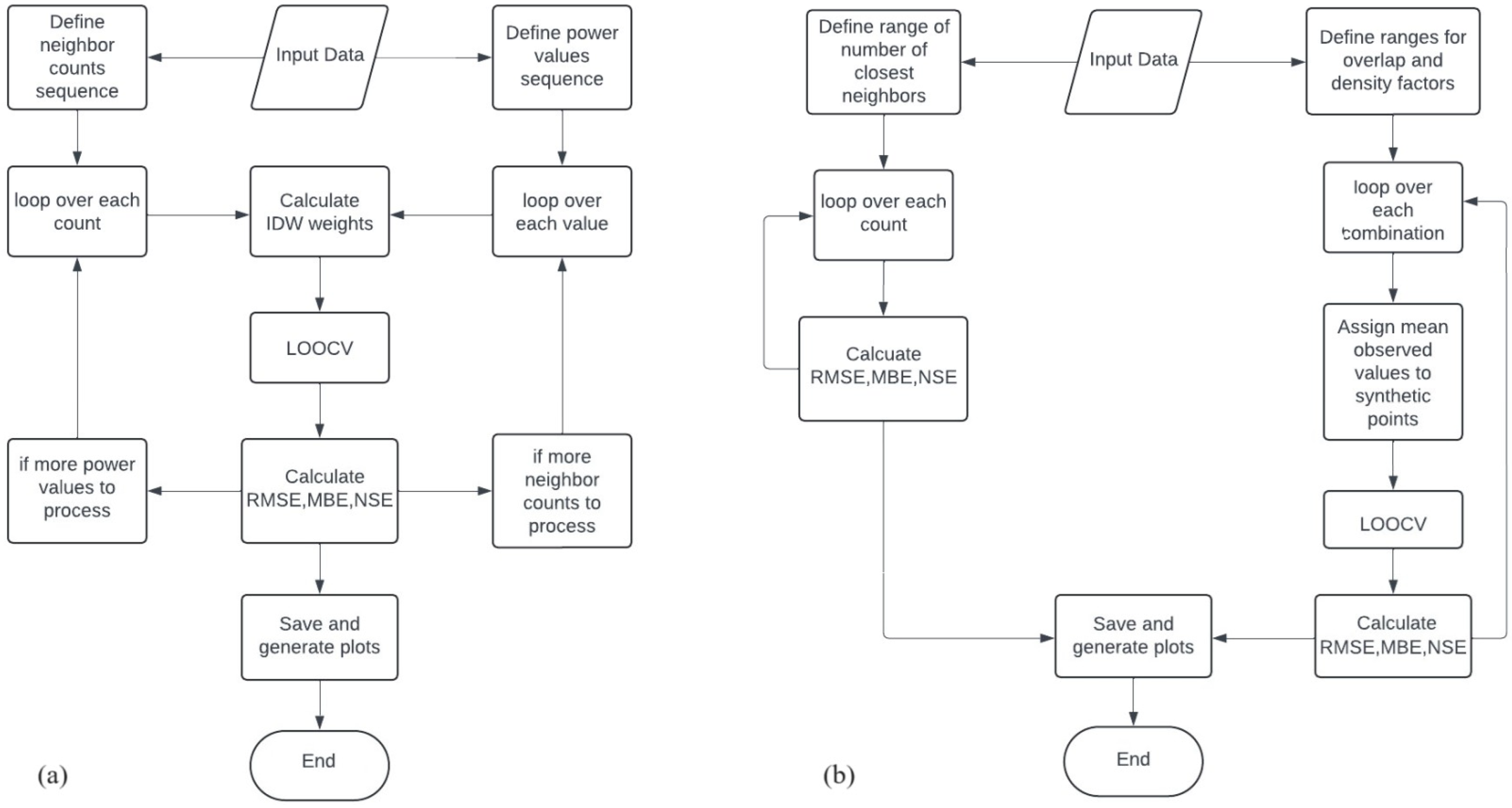
The flowchart of the sensitivity analysis is presented in Figure 3.

In the sensitivity analysis for IDW, the following aspects were considered:

• Varying the power parameter β, which determines the weight given to each data point based on its distance from the prediction site. This step involves varying β from 1 to 10 (in a sequence of 30 equidistant points);
• Consider a different number of neighbors included in the weighting process (2, 3, 4, 5, 6, 7, 8, 9, 10, 15, 20, 25, 30, 35, 40, 50, 60, and 70).

In the sensitivity analysis of BSS method, two directions were investigated:

• The number of closest data points included in calculating the mean values for PM_2.5 concentration to be assigned to the buffer points;
• The overlap and distribution of buffer points.

The overlap parameter (Overlap) is defined as a scaling factor extending the grid boundaries beyond their original extent. This parameter effectively enlarges the grid to include additional synthetic points along the edges and corners. Mathematically, the extended boundaries can be represented as

$$\begin{gathered} x_{min}^{new}=x_{min}-Overlap\times dx \\ {x}_{max}^{new}=x_{max}+Overlap\times dx \\ {y}_{min}^{new}=y_{min}-Overlap\times dy \\ {y}_{max}^{new}=y_{max}-Overlap\times dy, \end{gathered}$$

(12)

where $x_{min}$, $x_{max}$, $y_{min}$, and $y_{max}$ are the original boundaries of the grid, and $dx$ and $dy$ represent the original grid spacing in the $x$ and $y$ directions, respectively.

The density parameter (Density) modifies the spacing between these synthetic boundary points. A higher density factor results in more closely spaced synthetic points, increasing the granularity of the boundary extension. The new spacing between the synthetic points is given as follows:

$$\begin{gathered} {dx}_{new}=dx/Density, \\ {dy}_{new} =dy/Density \end{gathered}$$

(13)

where ${dx}_{new}$ and ${dy}_{new}$ are the adjusted spacings after applying the density factor.

This approach will help us address the local and global spatial relationships:

• The number of closest data points directly influences how the interpolation captures local spatial variations. Adjusting the number of closest points allows us to understand the balance between the local detail and the risk of incorporating noise or overfitting to local anomalies. It helps tailor the model to be sensitive to local spatial structures while maintaining general robustness;
• By experimenting with how buffer points are distributed and potentially overlap with the dataset, we are essentially modifying the model’s edge behavior and ability to extrapolate beyond the observed data domain. This can significantly affect the interpolation quality at the dataset’s boundaries, an area often prone to inaccuracies.

Different buffer point placement and overlap strategies can reveal insights into the best practices for ensuring smooth transitions at the boundaries, which is an important aspect for datasets with varying edge characteristics or when applying the model to new spatial domains with different boundary conditions. This adaptability of the model to different spatial domains underscores its versatility and potential for widespread application, a key aspect that should resonate with spatial analysts, GIS professionals, and researchers in environmental science and geospatial data analysis.

These two parameters cover both the local (immediate neighborhood relationships) and global aspects (boundary behavior) of spatial interpolation. This dual focus ensures that the model’s performance is optimized across the entire spatial domain, not just within the densely sampled areas. The sensitivity analysis focusing on these aspects will highlight the model’s robustness to variations in spatial sampling density and its flexibility in handling boundary conditions, both important for generalization across different spatial datasets. Furthermore, the insights gained from varying these parameters can guide the selection of optimal settings for future applications.

3. Results

3.1. Modeling Results

Figure 4 presents the charts of the MAE, RMSE, and MAPE across the grid points.

The average MAE, RMSE, and MAPE are lower for BSS compared to IDW. The values of NSE, KGE, and dIndex in the IDW and BSS interpolation are plotted in Figure 5 and Figure 6. Most are over 0.95, with a better concentration close to 1 for the BSS. Remark also the performances of the BSS on most of the grid edges (for example, 1–10, 20,21, 30, 31, 41, 50, 51, and 70).

When employing IDW, it is essential to factor in the distance from the target point to the neighboring points and the internal dataset similarity. The presence of positive spatial autocorrelation can significantly influence the IDW performance because the series in neighboring locations are more likely to have a higher impact and be more similar than those located at a greater distance. However, it is important to note that IDW’s performance is lower at the edges of the grid due to a smaller number of neighbors compared to those of the points inside the grid. This issue was addressed by introducing buffer points in BSS.

BSS’s spatial coherence and robustness are underlined by the values of dIndex and NSE (Figure 6), which are consistently observed across all points, including those situated in the corners and edges of the grid.

The Friedman test confirmed the BSS’s superiority, accounting for the goodness-of-fit indicators. This method’s strength does not depend on the spatial distribution of the grid points, which recommends it for various locations and the edge effect’s resilience.

3.2. Sensitivity Analysis of IDW

In the first stage of this analysis, the β parameter varied from 1 to 10 (usually considered in the IDW interpolation problems) in a sequence of 30 increments, and all the grid points were involved in the interpolation. Figure 7, Figure 8 and Figure 9 contain respectively:

• The RMSE and the Mean RMSE across the grid points vs. $\mathsf{\beta }$ (Figure 7);
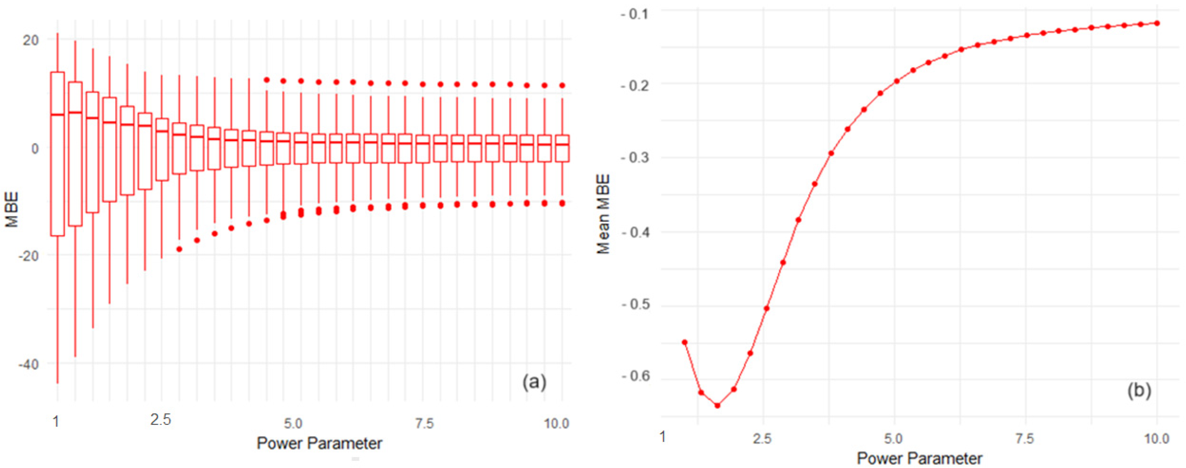
• The MBE vs. $\mathsf{\beta }$ and the Mean MBE vs. the $\mathsf{\beta }$. MBE is computed as the average of the difference between the estimated and recorded values (Figure 8);
• NSE distribution vs. $\mathsf{\beta }$; (b) Mean NSE vs. $\mathsf{\beta }$ (Figure 9).

Figure 7. (a) RMSE distribution as a function of $\mathsf{\beta }$. The dots represent the outliers; (b) Mean RMSE across the grid points vs. $\mathsf{\beta }$. The dots represent the Mean RMSE values.

Figure 7. (a) RMSE distribution as a function of $\mathsf{\beta }$. The dots represent the outliers; (b) Mean RMSE across the grid points vs. $\mathsf{\beta }$. The dots represent the Mean RMSE values.

Figure 8. (a) Mean bias error (MBE) vs. $\mathsf{\beta }$. The dots represent the outliers; (b) Mean MBE across stations vs. $\mathsf{\beta }$. The dots represent the Mean MBE value.

Figure 8. (a) Mean bias error (MBE) vs. $\mathsf{\beta }$. The dots represent the outliers; (b) Mean MBE across stations vs. $\mathsf{\beta }$. The dots represent the Mean MBE value.

Figure 9. (a) NSE distribution vs. $\mathsf{\beta }$. The dots represent the outliers; (b) Mean NSE across stations vs. $\mathsf{\beta }$. The dots represent the Mean NSE values.

Figure 9. (a) NSE distribution vs. $\mathsf{\beta }$. The dots represent the outliers; (b) Mean NSE across stations vs. $\mathsf{\beta }$. The dots represent the Mean NSE values.

The boxplots for goodness-of-fit indicators (Figure 7a, Figure 8a and Figure 9a) show the distribution of the error metrics across different power parameters. The RMSE and MBE boxplots reveal that error variability decreases as the power parameter increases up to a certain point, after which it remains almost constant. The NSE boxplot indicates that the model’s predictive power generally improves when $\mathsf{\beta }$ increases, with less variability of the NSE values at higher values of the power parameter. The outliers in the RMSE plot (Figure 7a) are particularly noticeable at lower power parameter values and suggest that the error can be significantly higher than the average for certain stations or specific datasets.

Figure 8 and Figure 9 indicate that the IDW scheme converges too slowly (with grid resolution) for some concentration distributions. The outliers in the MBE plot (Figure 8a) could also represent stations where the IDW method consistently overestimates or underestimates the observed values, regardless of the overall trend toward minimal bias. The spread of the outliers on both sides of zero indicates that while the method does not show a systematic bias, individual stations or data points may experience significant bias errors that do not follow the general trend.

Outliers in the NSE distribution (Figure 9a) indicate stations or conditions under which the model performance deviates substantially from the average efficiency. Negative outliers should be observed because they imply that for some stations, the mean of the observed data is a better predictor than the IDW interpolated values, signifying poor model performance. This underscores the need for further investigation into the conditions that lead to such outliers. Understanding these conditions can provide valuable insights into the limitations of the IDW method and potential areas for improvement.

Figure 7b emphasizes a clear decreasing trend of Mean RMSE as the power parameter increases from 1 to approximately 4 and then stabilizes with a further increase of $\mathsf{\beta }$. This behavior indicates a significant reduction in the prediction error as the power parameter increases from its lowest value until it reaches an optimal range.

Figure 8a indicates that the bias in prediction fluctuates around zero, with the lowest bias observed at a power parameter near 4. The bias is minimal in the optimal range, suggesting that the IDW method does not consistently overestimate or underestimate across the entire range of power parameters but has an optimal bias performance at a specific power value.

The NSE plot (Figure 9a) demonstrates an increasing trend with the power parameter, plateauing after a $\mathsf{\beta }$ value of about 4. A similar behavior is exhibited by the Mean NSE across stations as a function of $\mathsf{\beta }$ (Figure 9b). High NSE values (close to 1) indicate that the model’s predictions are very efficient in capturing the variance of the observed data, especially in the optimal range.

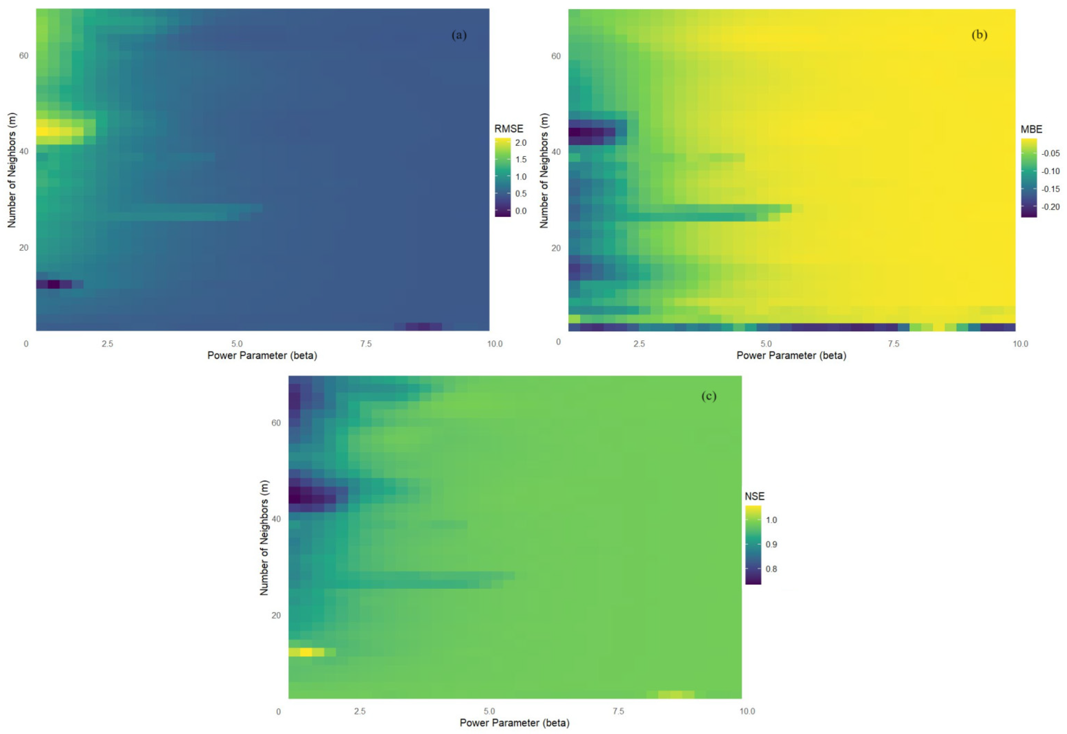
For the second point of the sensitivity analysis of IDW, we considered various numbers of neighbors participating in the interpolation process. First, we draw charts of the Mean RMSE, MBE, and NSE vs. the number of neighbors (Figure 10) and heatmaps (2D distributions) of RMSE, MSE, and NSE as functions of $\mathsf{\beta }$ and m (Figure 11).

We remark the following:

• The Mean RMSE is inversely related to the number of neighbors, at least up to a certain point. The highest RMSE is observed when the lowest number of neighbors (m = 2) is used, indicating the least accurate predictions with a Mean RMSE of about 6.5. There is a marked improvement in the prediction accuracy as the number of neighbors increases to m = 6, where the Mean RMSE drops to its lowest value of around 4.0. Beyond m = 7, the RMSE increases slightly to approximately 4.45 and then levels off, suggesting a plateau in model performance with additional neighbors providing no significant improvement in accuracy;
• The MBE plot shows that all values are negative, implying a consistent underestimation across different numbers of neighbors. The most pronounced bias occurs at m = 2 with a Mean MBE of around −2.3. There is a sharp improvement as m increases to 4, with Mean MBE rising to about −0.12. Interestingly, there is a slight increase in bias again at m = 6 before it settles back to approximately −0.2 at m = 7 and then stabilizes. This pattern suggests that the model bias is significantly reduced as neighbors are increased from the minimum, but only up to a point, after which the benefit diminishes;
• The lowest NSE value at m = 2 indicates a poor model performance relative to the mean of the observed data. As the number of neighbors increases to m = 6, there is a significant improvement in NSE to a peak of around 0.9605, suggesting that the model’s predictive accuracy is much better. However, the subsequent drop in NSE at m = 7 and the plateau after that suggest that including more than six neighbors does not substantially capture additional variability in the data;
• Figure 11a indicates that for β > 2.5, RMSE does not depend on m (at least for m > 4) because, in this case, only the nearest neighbors play a significant role in interpolation. For β > 4, most MBE values are between −0.05 and 0, indicating a suitable fit of the interpolation model. NSE is almost constant as a function of both parameters (Figure 11c) when β > 4. Significant RMSE, MBE, and NBE variations on both parameters appear only for β less than 2.3 and m between 42 and 50.

Secondly, the boxplots of each error metric are considered (Figure 12). Their analysis underlines the following aspects.

• The RMSE values (Figure 12a) tend to decrease as the number of neighbors increases, with the lowest spread (interquartile range) and the highest number of outliers at m = 6. The smallest box at this point suggests a more consistent model performance, albeit with some notable exceptions as indicated by the outliers. The largest RMSE and box size at m = 2 and fewer outliers indicate a higher average error and more significant variability. The medians being closer to the lower quartile across most boxes indicate a right-skewed distribution, with most of the data points having lower RMSE values and a few with substantially higher errors;
• The MBE boxplot (Figure 12b) indicates the presence of bias in predictions, with the most significant bias at m = 2, as demonstrated by the largest box and the median positioned toward the lower end of the range. The presence of outliers on both sides for various numbers of neighbors suggests that the model can both overestimate and underestimate to varying degrees but predominantly underestimate, as indicated by the negative means. As the number of neighbors increases beyond 6, the boxes stabilize in size, and the distribution of outliers becomes more symmetrical, suggesting a reduction in bias;
• The NSE boxplots (Figure 12c) reveal many outliers below the boxes, particularly at lower numbers of neighbors. The smallest box at m = 6 suggests the most consistent model efficiency, while the largest one at m =2 with the farthest outlier indicates the least efficient model predictions. The consistency in box size and outlier distribution for n > 6 suggests that the model efficiency does not significantly improve with more neighbors beyond this point.

3.3. BSS’ Sensitivity Analysis

For the first aspect (number of closest data points), we used different numbers of neighboring points (2, 3, 4, 5, 6, 7, 8, 10, 20, 25, 30, 35, 40, and 50) to calculate the mean PM_2.5 buffer point value. Then, we focused on three metrics that capture the different aspects of the model’s performance: RMSE, MBE, and NSE. Figure 13 contains the charts of these indicators as functions of the number of the closest points.

The RMSE plot shows a clear upward trend as the number of closest points increases. This suggests that incorporating more points into the mean calculation for buffer points leads to a general decrease in model accuracy. The initial low RMSE values indicate that fewer points may provide a better localized estimation, effectively capturing the immediate spatial variance. However, as more points are included, the increased RMSE could be due to the dilution of local specifics, incorporating broader spatial influences that may not be representative of the specific locations of the buffer points.

The MBE plot reveals an interesting pattern, where initially, the mean bias error increases with the number of points but then starts to plateau. The increasing trend suggests the model tends to systematically overestimate (positive MBE) the PM_2.5 values as more points are included. The leveling-off of the curve indicates that beyond a certain number of points, the bias introduced by including additional points does not significantly increase, suggesting a threshold beyond which further inclusion of points does not markedly change the mean bias.

The NSE plot exhibits a downward trend, indicating that the model’s ability to predict the variability of the observed data diminishes as the number of closest points increases. High NSE values with fewer points suggest that the model accurately captures the observed variability with a more localized approach. As the number of points increases, the decline in NSE may reflect a loss in capturing local variance due to averaging over a wider spatial area.

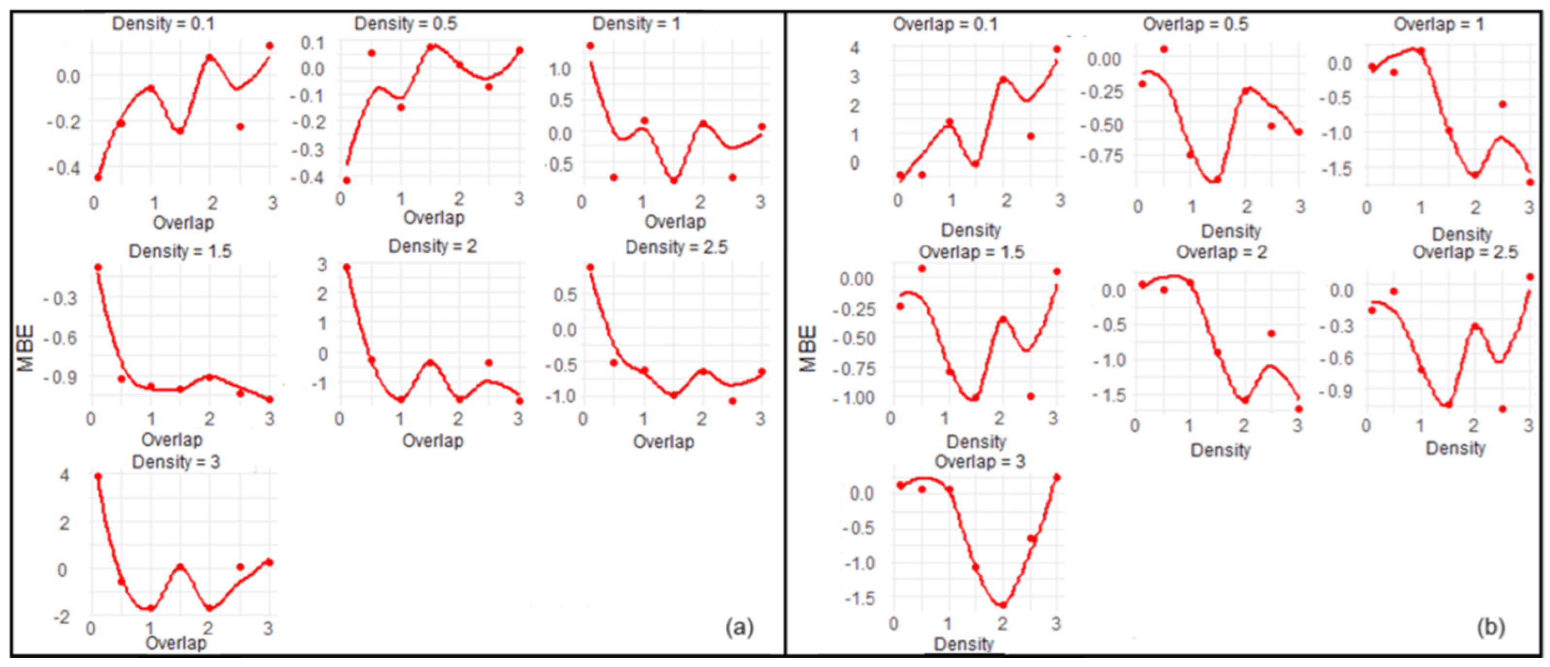
For the second point (the overlap and distribution of buffer points), we provided plots to illustrate the impact of overlap and density parameters on the performance of metrics RMSE, MBE, and NSE for BSS. Figure 14, Figure 15 and Figure 16 provide the following information:

• Lower RMSE values indicate a better fit of the model to the data. Figure 14 shows that certain levels of overlap and density consistently result in lower RMSE. Specifically, a lower density often corresponds to a lower RMSE, suggesting that a denser grid of buffer points may not always lead to more accurate interpolation. However, the relationship between overlap and RMSE is not as clear-cut and appears more variable across different densities;
• The MBE value provides insight into the model’s bias, with values closer to 0 indicating less bias. Figure 15 demonstrates the variability in bias across different levels of overlap and density. It seems that the model is sensitive to these parameters, and there is no single combination that consistently minimizes bias across all levels;
• Higher NSE values suggest better model predictive power. Figure 16 shows that specific combinations lead to higher NSE. The relationship appears complex, indicating that both parameters influence the predictive accuracy in a non-linear manner.

4. Discussion

4.1. Discussion about the Sensitivity Analysis of IDW

The sensitivity analysis proved that the IDW method has a specific power parameter range for optimizing the model’s performance. This assertion is evidenced by the reduction in RMSE and the leveling-off of MBE and NSE values. The optimal power parameter is around 4, where the RMSE is minimized and the NSE reaches a plateau, indicating efficient model predictions.

The reduction in the variability of the error metrics, particularly RMSE and MBE, at higher power parameters suggests that the model becomes less sensitive to the exact choice of the power parameter once it reaches the optimal range. This finding is beneficial for general application as it implies that the model is robust to some variation in the power parameter. Moreover, the consistent performance across a range of power parameters rather than at a single value is promising for generalizing the method to other datasets. It suggests that the model does not require precise tuning to perform reasonably.

Concluding, the IDW method exhibits sensitivity to the power parameter, with a marked improvement in prediction accuracy and bias as the β increases to an optimal range of about 4. Beyond this optimal range, the benefit of increasing the power parameter diminishes. However, before generalizing this method to other datasets, it is crucial to consider the spatial characteristics and distribution of the new data, as these factors can significantly influence the optimal power parameter selection.

In summary, the IDW method with β around 4 offers a balance between accuracy and generalizability, making it suitable for application to other spatial datasets. However, further validation with new data is recommended to confirm its broader applicability.

The outliers’ analysis in IDW leads to the following remarks:

• Sensitivity to Local Conditions: Outliers may suggest that the IDW method’s performance is particularly sensitive to local spatial characteristics, such as the variability modeled underlying physical processes. This sensitivity could affect the method’s generalizability to other datasets with different spatial characteristics.
• Model Robustness and Reliability: The existence of outliers, especially if they are numerous, can call into question the robustness and reliability of the IDW method. A robust model would ideally have fewer outliers, indicating consistent performance across different settings.
• Need for Model Adjustment or Supplemental Methods: Outliers may indicate the need for additional model adjustments or the incorporation of supplemental methods to handle spatial anomalies or extreme values. They could include preprocessing steps to normalize data, remove noise, or account for non-stationarity in the data.

IDW interpolation reveals a non-linear relationship between the number of neighbors and the error metrics. RMSE and NSE improve as more neighbors are considered, up to m = 6, which could be due to the increased sample size contributing more relevant information for prediction, thereby reducing error and improving efficiency. However, the plateau in RMSE and NSE values beyond m = 7 indicates that including too many neighbors may introduce noise or redundant information that does not contribute to prediction accuracy. The MBE results suggest that the model has a tendency for underestimation, which is mitigated by increasing the neighbors, but only to a certain extent.

The optimal number of neighbors for the IDW interpolation is around m = 6, minimizing RMSE and maximizing NSE without introducing significant bias. The initial underestimation bias (negative MBE) reduces sharply as more neighbors are included, but it does not entirely disappear. The plateau observed in all metrics beyond m = 7 suggests that further increasing the number of neighbors does not yield additional benefits and could even be counterproductive. These insights can be used to refine the model and guide the selection of an appropriate neighborhood size for future predictions, balancing accuracy and computational efficiency.

The boxplots corroborate the trends observed in the mean plots. The IDW model’s performance improves markedly with the increase in the number of neighbors up to m = 6, as evidenced by the reduction in RMSE and MBE and the increase in NSE. However, there is significant variability in model performance, particularly with fewer neighbors, as shown by the outliers. This variability could be due to the influence of specific local conditions at individual stations or anomalous data points that do not follow the general trend. The error metrics suggest that the IDW model is sensitive to the choice of neighbors, with too few neighbors leading to high variability and bias in predictions. However, there is an optimal neighborhood size (m = 6) beyond which increasing the number of neighbors does not yield substantial improvements and could potentially introduce noise.

Concluding, IDW exhibits distinct sensitivities to the power parameter and the number of neighbors. Optimal values for these parameters have been identified for the analyzed dataset, suggesting that the model’s performance is contingent on fine-tuning these parameters. For generalization to other datasets, the following points are critical:

• Dataset Characteristics: Generalization is more feasible for datasets with similar spatial and variable characteristics;
• Outlier Management: The model’s predictability can be affected by outliers, necessitating robust outlier handling for new datasets;
• Spatial Correlation: The assumption of spatial autocorrelation inherent in IDW must hold for the target dataset;
• Parameter Reevaluation: Parameter optimization is dataset-specific and should be reevaluated for each new dataset;
• Validation: Independent validation is essential to ascertain the model’s predictive capability across datasets.

4.2. Discussion about the Sensitivity Analysis of BSS

The number of closest points used for buffer point PM_2.5 value calculation significantly impacts the interpolation’s accuracy, bias, and efficiency. Fewer points tend to offer better local accuracy and efficiency in capturing the variability of the observed data, as indicated by the lower RMSE and higher NSE. However, too few points may introduce bias, as indicated by the initial increase in MBE. There appears to be a trade-off between bias and accuracy, which suggests an optimal range of closest points that balances these metrics.

The optimal number of closest points for buffer assignment should be chosen to minimize RMSE and MBE while maximizing NSE, considering the specific context and requirements of the spatial analysis. This balance ensures that the model is neither overfitting to local data nor overly smoothing out significant local spatial variations. The analysis suggests that a more moderate number of closest points might balance local detail fidelity and general smoothness. However, the specific optimal point will depend on the context of the data and the spatial patterns present in the specific application.

In practice, these insights guide fine-tuning Bicubic Spline Smoothing methods when applied to different datasets, enhancing their generalization potential. The conclusions drawn from this sensitivity analysis can help inform decisions on method configuration for future spatial interpolation tasks, aiming to achieve reliable and accurate predictions.

Finally, to choose the optimal number of closest points (for our present dataset), we applied a Bayesian optimization approach to maximize the score function defined by:

score = − RMSE − MBE + NSE.

The result showed that the optimal value for closest points is 2, implying that for our specific spatial data and interpolation task, a tighter local neighborhood captures the necessary detail more accurately without introducing the noise or error that might come with broader averaging.

The sensitivity analysis that took into account the overlap and distribution of buffer points indicates that the best combinations to ensure the model performance are the following:

• For minimizing RMSE, a lower density should be the choice, regardless of the overlap;
• For MBE, the least bias is observed at medium density and lower overlap levels;
• The optimal NSE values are found at lower levels of overlap across most densities, with certain exceptions at higher densities where the pattern is less clear.

Combined with the results from the first step of the sensitivity analysis (number of closest points), these findings contribute to understanding the model’s robustness. Based on a Bayesian optimization approach, the initial analysis suggested that fewer closest points (e.g., two) could result in a better-performing model. The results suggest that the BSS’s performance is sensitive to the choice of both buffer parameters and the number of closest points. While we can identify specific settings that optimize the performance metrics, the variability across different levels of overlap and density, coupled with the optimal number of closest points, indicates that the model may not be easily generalizable across all datasets without careful tuning these parameters.

The best generalization values would be those that consistently perform well across different datasets. The current analysis does not provide enough evidence to conclusively state that the model can be generalized because it is based on a single dataset. For a robust claim of generalizability, the model must be tested on multiple datasets with varying characteristics to ensure that the identified optimal parameter settings hold in different contexts.

The study considered model-calculated spatial fields of PM_2.5. Even with data assimilation, these are not equivalent to real fields, which may be characterized by higher inhomogeneity, sharper gradients, etc. So, this study’s findings apply to interpolating gridded model-calculated products. Still, it can also be extended to real data series.

5. Conclusions

In this article, we assessed the sensitivity of the interpolation models built using IDW and BSS for the MERRA-2 reanalysis PM_2.5 monthly gridded series from the UAE region.

The results suggest that the IDW method’s performance is relatively stable within a specific range of the power parameter (β), but its generalizability may be influenced by the specific spatial characteristics of the dataset. The optimal number of neighbors for the IDW model was 6, striking a balance between reducing the error and increasing the model efficiency. The presence of outliers suggests that the model could benefit from further refinement or incorporating additional data processing steps to handle anomalous values more effectively. Further research and validation are recommended to confirm the IDW method’s broader applicability and explore how it can be adapted or enhanced to handle the diversity of spatial datasets encountered in practice.

The BSS model’s sensitivity study provides valuable insights for interpolation method performance but may not hold universally. Further validation across diverse datasets is recommended to ensure the generalizability of the model.

References

1. Nazzal, Y.; Bou Orm, N.; Bărbulescu, A.; Howari, F.; Sharma, M.; Badawi, A.; Al-Taani, A.A.; Iqbal, J.; El Ktaibi, F.; Xavier, C.M.; et al. Study of atmospheric pollution and health risk assessment. A case study for the Sharjah and Ajman Emirates (UAE). Atmosphere 2021, 12, 1442. [Google Scholar] [CrossRef]
2. Bărbulescu, A.; Dumitriu, C.S.; Ilie, I.; Barbeș, S.B. Influence of Anomalies on the Models for Nitrogen Oxides and Ozone Series. Atmosphere 2022, 13, 558. [Google Scholar] [CrossRef]
3. Bărbulescu, A.; Dumitriu, C.S.; Popescu-Bodorin, N. On the aerosol optical depth series in the Arabian Gulf region. Rom. J. Phys. 2022, 67, 814. [Google Scholar]
4. Bărbulescu, A.; Barbeș, L.; Dumitriu, C.Ș. Advances in Water, Air and Soil Pollution Monitoring, Modeling and Restoration. Toxics 2024, 12, 244. [Google Scholar] [CrossRef] [PubMed]
5. Inhalable Particulate Matter and Health (PM2.5 and PM10). Available online: https://ww2.arb.ca.gov/resources/inhalable-particulate-matter-and-health (accessed on 15 January 2024).
6. Chiritescu, R.-V.; Luca, E.; Iorga, G. Observational study of major air pollutants over urban Romania in 2020 in comparison with 2019. Rom. Rep. Phys. 2024, 76, 702. [Google Scholar]
7. Dumitru, A.; Olaru, E.-A.; Dumitru, M.; Iorga, G. Assessment of air pollution by aerosols over a coal open-mine influenced region in southwestern Romania. Rom. J. Phys. 2024, 69, 801. [Google Scholar] [CrossRef]
8. Gon Ryou, H.; Heo, J.; Kim, S.Y. Source apportionment of PM10 and PM2.5 air pollution, and possible impacts of study characteristics in South Korea. Environ. Pollut. 2018, 240, 963–972. [Google Scholar] [CrossRef] [PubMed]
9. Arias-Pérez, R.D.; Taborda, N.A.; Gómez, D.M.; Narvaez, J.F.; Porras, J.; Hernandez, J.C. Inflammatory effects of particulate matter air pollution. Environ. Sci. Pollut. Res. 2020, 27, 42390–42404. [Google Scholar] [CrossRef] [PubMed]
10. Saliba, Y.; Bărbulescu, A. A comparative evaluation of spatial interpolation techniques for maximum temperature series in the Montreal region. Rom. Rep. Phys. 2024, 76, 701. [Google Scholar]
11. Popescu-Bodorin, N.; Bărbulescu, A. A ten times smaller version of CPC Global Daily Precipitation Dataset for parallel distributed processing in Matlab and R. Rom. Rep. Phys. 2024, 76, 703. [Google Scholar]
12. Thangavel, P.; Park, D.; Lee, Y.C. Recent Insights into Particulate Matter (PM2.5)-Mediated Toxicity in Humans: An Overview. Int. J. Environ. Res. Public Health 2022, 19, 7511. [Google Scholar] [CrossRef] [PubMed]
13. Estimate of Premature Deaths Associated with Fine Particle Pollution (PM2.5) in California Using a U.S. Environmental Protection Agency Methodology. Available online: https://archive.epa.gov/region9/mediacenter/web/pdf/pm-report_2010.pdf (accessed on 12 January 2024).
14. Nazzal, Y.; Bărbulescu, A.; Howari, F.M.; Yousef, A.; Al-Taani, A.A.; Al Aydaroos, F.; Naseem, M. New insight to dust storm from historical records, UAE. Arab. J. Geosci. 2019, 12, 396. [Google Scholar] [CrossRef]
15. Nazzal, Y.; Bărbulescu, A. Statistical analysis of the dust storms in the United Arab Emirates. Atmos. Resear. 2020, 231, 104669. [Google Scholar]
16. How Bad Is Our Air Pollution—And How Do We Tackle It? Available online: https://www.thenationalnews.com/uae/environment/2022/09/20/explained-how-much-of-a-problem-is-air-pollution-in-the-uae/ (accessed on 20 April 2024).
17. You Can Smell Petrol in the Air. 2023. Available online: https://www.hrw.org/report/2023/12/04/you-can-smell-petrol-air/uae-fossil-fuels-feed-toxic-pollution#:~:text=The%20UAE%20has%20dangerously%20high,considers%20safe%20for%20human%20health (accessed on 20 April 2024).
18. OECD. Air Pollution Exposure (Indicator). 2024. Available online: https://data.oecd.org/air/air-pollution-exposure.htm#indicator-chart (accessed on 15 May 2024).
19. Liu, H.; Zhang, S.; Liu, L.; Yu, J.; Ding, B. A Fluffy Dual-Network Structured Nanofiber/Net Filter Enables High-Efficiency Air Filtration. Adv. Funct. Mater. 2019, 29, 1904108. [Google Scholar] [CrossRef]
20. Victor, F.S.; Kugarajah, V.; Bangaru, M.; Ranjan, S.; Dharmalingam, S. Electrospun nanofibers of polyvinylidene fluoride incorporated with titanium nanotubes for purifying air with bacterial contamination. Environ. Sci. Pollut. Res. Int. 2021, 28, 37520–37533. [Google Scholar] [CrossRef] [PubMed]
21. Beaver, S.; Palazoglu, A. Influence of synoptic and mesoscale meteorology on ozone pollution potential for San Joaquin Valley of California. Atmos. Environ. 2021, 247, 118063. [Google Scholar] [CrossRef]
22. Li, L.; Losser, T.; Yorke, C.; Piltner, R. Fast inverse distance weighting-based spatiotemporal interpolation: A web-based application of interpolating daily fine particulate matter PM2.5 in the contiguous U.S. using parallel programming and k-d tree. Int. J. Environ. Res. Public Health 2014, 11, 9101–9141. [Google Scholar] [CrossRef] [PubMed]
23. Choi, K.; Chong, K. Modified Inverse Distance Weighting Interpolation for Particulate Matter Estimation and Mapping. Atmosphere 2022, 13, 846. [Google Scholar] [CrossRef]
24. Deng, L. Estimation of PM2.5 Spatial Distribution Based on Kriging Interpolation. In Proceedings of the First International Conference on Information Sciences, Machinery, Materials and Energy, Chongqing, China, 11–13 April 2015; pp. 1791–1794. [Google Scholar]
25. Diggle, P.J.; Ribeiro, P.J. Model-Based Geostatistics; Springer Science & Business Media: Berlin/Heidelberg, Germany, 2007. [Google Scholar]
26. Lee, S.J.; Serre, M.L.; van Donkelaar, A.; Martin, R.V.; Burnett, R.T.; Jerrett, M. Comparison of geostatistical interpolation and remote sensing techniques for estimating long-term exposure to ambient PM2.5 concentrations across the continental United States. Environ. Health Perspect. 2012, 120, 1727–1732. [Google Scholar] [CrossRef]
27. Wei, P.; Xie, S.; Huang, L.; Liu, L.; Tang, Y.; Zhang, Y.; Wu, H.; Xue, Z.; Ren, D. Spatial interpolation of PM2.5 concentrations during holidays in south-central China considering multiple factors. Sci. Total Environ. 2020, 740, 139761. [Google Scholar] [CrossRef]
28. Oshan, T.M.; Li, Z.; Kang, W.; Wolf, L.J.; Fotheringham, A.S. Mgwr: A Python implementation of multiscale geographically weighted regression for investigating process spatial heterogeneity and scale. ISPRS Int. J. Geo-Inf. 2019, 8, 269. [Google Scholar] [CrossRef]
29. Yanosky, J.D.; Paciorek, C.J.; Suh, H.H. Predicting chronic fine and coarse particulate exposures using spatiotemporal models for the Northeastern and Midwestern United States Environ. Health Perspect. 2009, 117, 522–529. [Google Scholar] [CrossRef] [PubMed]
30. Saliba, Y.; Bărbulescu, A. Downscaling MERRA-2 Reanalysis PM2.5 Series over the Arabian Gulf by Inverse Distance Weighting, Bicubic Spline Smoothing, and Spatio-Temporal Kriging. Toxics 2024, 12, 177. [Google Scholar] [CrossRef] [PubMed]
31. Gräler, B.; Pebesma, E.; Heuvelink, G. Spatio-Temporal Interpolation using gstat. R J. 2016, 8, 204–218. [Google Scholar] [CrossRef]
32. Goudarzi, G.; Hopke, P.H.; Yazdani, M. Forecasting PM2.5 concentration using and its health effects in Ahvaz, Iran. Chemosphere 2021, 283, 131285. [Google Scholar] [CrossRef]
33. Ma, J.; Ding, Y.; Cheng, J.C.P.; Jiang, F.; Wan, Z. A temporal-spatial interpolation and extrapolation method based on geographic Long Short-Term Memory neural network for PM2.5. J. Clean. Prod. 2019, 237, 117729. [Google Scholar] [CrossRef]
34. Xiao, F.; Yang, M.; Fan, H.; Fan, G. An improved deep learning model for predicting daily PM2.5 concentration. Sci. Rep. 2020, 10, 20988. [Google Scholar] [CrossRef] [PubMed]
35. Chae, S.; Shin, J.; Kwon, S.; Lee, S.; Kang, S.; Lee, D. PM10 and PM2.5 real-time prediction models using an interpolated convolutional neural network. Sci. Rep. 2021, 11, 11952. [Google Scholar] [CrossRef]
36. Rizos, K.; Meleti, C.; Evagelopoulos, V.; Melas, D. A machine learning modelling approach to characterize the background pollution in the Western Macedonia region in northwest Greece. Atmos. Pollut. Resear. 2023, 14, 101877. [Google Scholar] [CrossRef]
37. Zoras, S.; Evagelopoulos, V.; Pytharoulis, I.; Triantafyllou, A.G.; Skordas, I.; Kallos, G. Development and validation of a novel-based combination operational air quality forecasting system in Greece. Meteorol. Atmos. Phys. 2010, 106, 127–133. [Google Scholar] [CrossRef]
38. Mahajan, S.; Chen, L.-J.; Tsai, T.-C. Short-Term PM2.5 Forecasting Using Exponential Smoothing Method: A Comparative Analysis. Sensors 2018, 18, 3223. [Google Scholar] [CrossRef] [PubMed]
39. Zhou, Z.H. Ensemble Methods: Foundations and Algorithms; Chapman and Hall/CRC: Boca Raton, FL, USA, 2012. [Google Scholar]
40. Li, X.; Peng, L.; Yao, X.; Cui, S.; He, W. Integrating remote sensing data with ground-based measurements to improve air quality mapping. Remote Sens. Environ. 2016, 184, 212–221. [Google Scholar]
41. Shao, Y.; Ma, Z.; Wang, J.; Bi, J. Estimating daily ground-level PM2.5 in China with random-forest-based spatiotemporal kriging. Sci. Total Environ. 2020, 740, 13761. [Google Scholar] [CrossRef]
42. Liu, H.; Chen, C. Prediction of outdoor PM2.5 concentrations based on a three-stage hybrid neural network model. Atmos. Pollut. Res. 2020, 11, 469–481. [Google Scholar] [CrossRef]
43. Wang, Y.; Di, Q.; Liu, Y. Hybrid deep learning model for PM2.5 prediction. Atmos. Environ. 2019, 212, 5–10. [Google Scholar]
44. Chatzinikolaou, E.; Nikolopoulos, K. A hybrid statistical and machine learning model for air quality prediction. J. Environ. Manag. 2019, 237, 28–38. [Google Scholar]
45. MERRA-2 tavgM_2d_aer_Nx: 2d, Monthly Mean, Time-Averaged, Single-Level, Assimilation, Aerosol Diagnostics V5.12.4 (M2TMNXAER). Available online: https://disc.gsfc.nasa.gov/datasets/M2TMNXAER_5.12.4/summary#citation (accessed on 15 May 2024).
46. Gelaro, R.; McCarty, W.; Suárez, M.J.; Todling, R.; Molod, A.; Takacs, L.; Randles, C.A.; Darmenov, A.; Bosilovich, M.G.; Reichle, R.; et al. The Modern-Era Retrospective Analysis for Research and Applications, Version 2 (MERRA-2). J. Clim. 2017, 30, 5419–5454. [Google Scholar] [CrossRef]
47. Li, J.; Heap, A.D. Spatial interpolation methods applied in the environmental sciences: A review. Environ. Modell. Softw. 2014, 53, 173–189. [Google Scholar] [CrossRef]
48. Paramasivam, C.; Venkatramanan, S. Chapter 3—An Introduction to Various Spatial Analysis Techniques. In GIS and Geostatistical Techniques for Groundwater Science; Venkatramanan, S., Prasanna, M.V., Chung, S.Y., Eds.; Elsevier: Amsterdam, The Netherlands, 2019; pp. 23–30. [Google Scholar]
49. De Bohr, C. Bicubic Spline Interpolation. J. Math. Phys. 1962, XLI, 212–218. [Google Scholar] [CrossRef]
50. Friedman, M. The use of ranks to avoid the assumption of normality implicit in the analysis of variance. J. Am. Stat. Assoc. 1938, 32, 675–701. [Google Scholar] [CrossRef]
Figure 1. The positions and coordinates of the sites.
Atmosphere 15 00748 g001
Figure 2. The series from the grid points 60–70.
Atmosphere 15 00748 g002
Figure 3. The flowchart of the sensitivity analysis for (a) IDW and (b) BSS. LOOCV means leave-one-out crossvalidation.
Atmosphere 15 00748 g003
Figure 4. (a) MAE, (b) RMSE, and (c) MAPE across the grid points for the optimum parameters, according to [30].
Atmosphere 15 00748 g004
Figure 5. (a) NSE, (b) KGE, and (c) dIndex across the grid points for IDW.
Atmosphere 15 00748 g005
Figure 6. (a) NSE, (b) KGE, and (c) dIndex across the grid points for BSS.
Atmosphere 15 00748 g006
Figure 10. Results of the sensitivity analysis for IDW: (a) Mean RMSE vs. the number of neighbors; (b) Mean MBE vs. the number of neighbors; (c) Mean NSE vs. the number of neighbors (the optimal beta was used for the representation).
Atmosphere 15 00748 g010
Figure 11. Heatmaps of (a) RMSE, (b) MBE, and (c) NSE in IDW.
Atmosphere 15 00748 g011
Figure 12. Results of the sensitivity analysis for IDW. Boxplots of (a) RMSE vs. the number of neighbors; (b) Mean MBE vs. the number of neighbors; (c) Mean NSE vs. the number of neighbors.
Atmosphere 15 00748 g012
Figure 13. (a) RMSE vs. the number of closest points; (b) Mean MBE vs. the number of closest points; (c) Mean NSE vs. the number of closest points.
Atmosphere 15 00748 g013
Figure 14. RMSE (a) across overlaps for different densities; (b) across densities for different overlaps.
Atmosphere 15 00748 g014
Figure 15. MBE (a) across overlaps for different densities; (b) across densities for different overlaps.
Atmosphere 15 00748 g015
Figure 16. NSE (a) across overlaps for different densities; (b) across densities for different overlaps.
Atmosphere 15 00748 g016
Disclaimer/Publisher’s Note: The statements, opinions and data contained in all publications are solely those of the individual author(s) and contributor(s) and not of MDPI and/or the editor(s). MDPI and/or the editor(s) disclaim responsibility for any injury to people or property resulting from any ideas, methods, instructions or products referred to in the content.