Abstract
Establishing reliable and effective prediction models is a major research priority for air quality parameter monitoring and prediction and is utilized extensively in numerous fields. The sample dataset of air quality metrics often established has missing data and outliers because of certain uncontrollable causes. A broad learning system based on a semi-supervised mechanism is built to address some of the dataset’s data-missing issues, hence reducing the air quality model prediction error. Several air parameter sample datasets in the experiment were discovered to have outlier issues, and the anomalous data directly impact the prediction model’s stability and accuracy. Furthermore, the correlation entropy criteria perform better when handling the sample data’s outliers. Therefore, the prediction model in this paper consists of a semi-supervised broad learning system based on the correlation entropy criterion (CC-SSBLS). This technique effectively solves the issue of unstable and inaccurate prediction results due to anomalies in the data by substituting the correlation entropy criterion for the mean square error criterion in the BLS algorithm. Experiments on the CC-SSBLS algorithm and comparative studies with models like Random Forest (RF), Support Vector Regression (V-SVR), BLS, SSBLS, and Categorical and Regression Tree-based Broad Learning System (CART-BLS) were conducted using sample datasets of air parameters in various regions. In this paper, the root mean square error (RMSE) and mean absolute percentage error (MAPE) are used to judge the advantages and disadvantages of the proposed model. Through the experimental analysis, RMSE and MAPE reached 8.68 μg·m−3 and 0.24% in the Nanjing dataset. It is possible to conclude that the CC-SSBLS algorithm has superior stability and prediction accuracy based on the experimental results.
1. Introduction
Predicting air quality requires the use of several airborne parameter indicators. To create models for predicting the changes in air quality over time, researchers employ statistical analysis [1,2] and machine learning approaches [3,4]. Prediction accuracy is often increased by combining many algorithms and utilizing techniques like feature engineering and model modification.
In the early days, traditional models were used to predict air quality. Traditional air quality prediction techniques include the Multi-scale Air Quality Model (CMAQ) [5], autoregressive moving average model (ARMA) [6], autoregressive integrated moving average model (ARIMA) [7], time series regression model [8], etc. Peng Sijun et al. [9] constructed a time-segment autoregressive integral moving average (ARIMA) prediction model to predict the air quality of the last day of different time periods. The experimental results show that the model has a good forecasting effect for air quality. Zhang et al. [10] also constructed the ARIMA prediction model and further expanded the dataset. The results show that the model has a better fitting effect and prediction accuracy. Hu et al. [11] combined the Weather Research and Prediction Model (WRF) and CMAQ model to conduct a one-year simulation study on air quality in China. The results demonstrate that the CMAQ model can reproduce PM2.5 concentrations in most cities. Although the above model has the advantages of simple principles, fast prediction speed, and good short-term data prediction of air quality, it is not suitable for long-term data prediction and nonlinear series analysis. Machine learning is a method to enter data into the network for nonlinear fitting to find the best solution, which can solve the drawbacks of traditional prediction methods and improve prediction accuracy. Liang et al. [12] used a single random forest model to predict the Air Quality Index (AQI) in three different regions, and the prediction accuracy was improved to a certain extent compared with the traditional statistical model. Ghaemi et al. [13] proposed an online nuclear classifier (LaSVM) for predicting urban air quality in Tehran, Iran, and compared the performance of this system to that of a traditional SVM, concluding that its significant advantage is that by removing nonsupport vector samples in the training step, processing time is significantly reduced, and accuracy is not compromised. Liu et al. [14] established a support vector regression (SVR) model to predict the AQI of the Beijing dataset, established a random forest regression (RFR) model to predict the nitrogen oxide (NOx) concentration of Italian cities, and finally concluded that the prediction effects of the SVR and RFR models were significantly better than that of classical regression models.
With the development of machine learning, deep learning algorithms are gradually being applied to air quality prediction. Zhang et al. [15] predicted the concentration of Hong Kong’s air quality through an extreme learning machine (ELM) based on eight types of air quality data from two monitoring stations in Hong Kong. The model has achieved good results in predicting air quality. Jiang et al. [16] improved the pigeon-inspired optimization algorithm by using the particle swarm optimization algorithm and then used the improved algorithm to optimize ELM. The Air Quality Index of Harbin city is used to verify the proposed method, and the results show that the method has good forecasting effect. Qiao et al. [17], based on RF models, designed a model combining the improved ant colony algorithm, and a BP neural network was used to predict the AQI data; the experimental results showed that the model achieved better results than the single RF model. Feng et al. [18] used the RNN model to predict the AQI in the first 24 h, and compared the experimental results with an RF model, finding that the prediction accuracy of the RNN model was higher. Belavadi et al. [19] combined Long Short-Term Memory (LSTM) with an RNN model to construct the LSTM–RNN model to complete the air quality prediction, and the prediction results have a high accuracy. In order to anticipate PM2.5 levels in Beijing, Zhang et al. [20] created a deep learning model that combines Variational Mode Decomposition (VMD) with Bidirectional Long Short-Term Memory (BiLSTM). This model greatly increases prediction accuracy. These models do a decent job of capturing the temporal characteristics of the data, but they are not as good at capturing the spatial correlations. Convolutional Neural Networks (CNN) were utilized by Qin et al. [21] to extract spatial features from raw data. These features were then fed into an LSTM model for prediction, yielding accurate forecasting outcomes. The Multi-Scale Spatial–Temporal Network (MSSTN), a novel deep Convolutional Neural Network model created by Wu et al. [22], increased prediction accuracy. Han et al. [23] proposed a multi-adversarial spatiotemporal recurrent graph neural network (masterergnn), which effectively suppressed the observation noise caused via spatiotemporal modeling and further improved the prediction accuracy. Scientists have made significant progress in the area of air quality prediction using deep learning. But as the networks get more complicated, there are also more hyperparameters to tweak, which means that training takes longer and uses more resources. Furthermore, tiny- to medium-sized datasets are not as well modeled via deep learning systems.
Chen et al. [24] created a broad learning system (BLS) to address the problem of model hyperparameters, enhancing the prediction accuracy of small- to medium-sized datasets and decreasing training time and computer resource utilization. Based on random vector functional linking, BLS is a learning network. BLS has a straightforward general structure, and experiments on small- to medium-sized datasets have demonstrated the algorithm’s benefits of high prediction accuracy and quick training speed. Scholars have studied the BLS algorithm in more detail in the last few years. An enhanced BLS structure based on K-means feature extraction was proposed by Liu et al. [25], and it shows good prediction performance while handling more complicated datasets. A model that integrates the broad learning system (BLS) with Classification and Regression Trees (CART) was developed by Wang et al. [26]. Through the division of the dataset’s features into more specialized subsets, this approach generates numerous subsets of data pertaining to particular attributes. The original dataset is utilized to train the global model, and these subsets are fed into the BLS network to train the local models. By doing this, a global-local model is produced that successfully resolves the global–local modeling duality issue and improves PM2.5 forecast accuracy even more.
It was discovered during the tests that several regional sample datasets had outliers and some data were missing because of uncontrollable circumstances impacting continuous data collecting. The stability and accuracy of the prediction models built with the aforementioned algorithms would decline in these kinds of scenarios. The SSBLS technique was developed as a semi-supervised mechanism in combination with BLS to handle the problem of partial data missing in the sample dataset. Outliers were found when several regional sample datasets were analyzed, and this had an immediate effect on the stability and precision of air quality prediction models. A semi-supervised broad learning system based on the related entropy criteria was developed as a result of the mean square error criterion in SSBLS being substituted with the related entropy criterion in order to address the outlier issue in the sample data [27,28]. Through comparison studies, this approach was applied to several region-specific sample datasets and compared with models such as RF, V-SVR, BLS, SSBLS, CART-BLS, and others. The outcomes of the trial showed that CC-SSBLS had superior accuracy and stability.
The contributions made in this paper are:
- (1)
- Four regional air quality datasets were established and four regional meteorological datasets were evaluated from Xuzhou, Nanjing, Beijing, and Changchun City (China);
- (2)
- The semi-supervised criteria and the correlation entropy criterion serve as the foundation for the CC-SSBLS prediction model, which is suggested with the goal of addressing the partially missing data and outlier problems in the air quality dataset. When the CC-SSBLS method is used on the air quality dataset spanning four locations, the experimental findings demonstrate that it is effective in resolving the dataset’s outlier and data-missing issues as well as improving the stability and prediction accuracy of the algorithm;
- (3)
- Air quality datasets from four different regions were subjected to CC-SSBLS application along with RF, V-SVR, BLS, SSBLS, and CART-BLS models. Stability and accuracy comparison experiments were also carried out, and the outcomes demonstrated that the CC-SSBLS algorithm performed better in terms of both stability and prediction accuracy.
The structure of the article is as follows. Section 1: introduces the current research status and background of air quality prediction. Section 2: elaborates on the principles of the algorithm used in this article. Section 3: presents experimental results and conducts comparative analysis. Section 4: draws the final conclusion.
2. Algorithm
2.1. BLS
The random vector function link neural network serves as the foundation for BLS [24] construction. On the one hand, feature nodes in the BLS network are created via feature mapping. However, augmentation nodes are added to the BLS network in order to boost its nonlinearities. The BLS structure diagram is shown in Figure 1. As the first step, the input data X are sent to the input layer, and feature mapping is performed to obtain the mapped feature , where are a randomly generated feature layer weight. represents the function calculation formula. The first n sets of feature mappings are concatenated as . The mapped features are augmented in the second step to obtain the augmented node , where and represent the weights randomly generated with the enhancement layer, and represents the function calculation formula. The first m groups of enhanced nodes are . The third step feeds the results of mapped features and enhanced nodes into the output layer to obtain
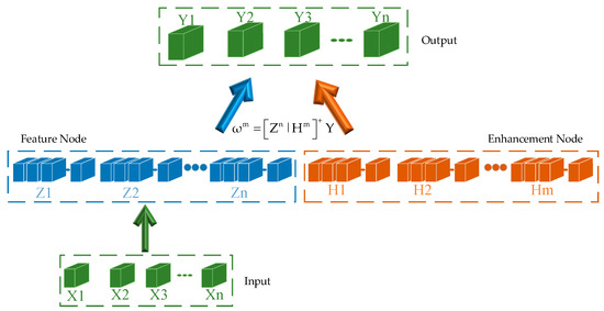
Figure 1.
BLS network operation principle diagram.
2.2. SSBLS
A semi-supervised BLS was introduced because the BLS algorithm did not achieve the expected prediction due to the large amount of missing valuable information contained in the dataset and the lack of data labels. The smoothing assumption underlies the semi-supervised algorithm. In [29], the smoothing assumption is imposed on the sample by minimizing Equation (1).
where is the pairwise similarity coefficient between and . However, in practice, it is difficult to calculate the conditional probability densities, so Equation (1) can be optimized as
where and in the formula are the predicted results corresponding to samples and . In [29], Equation (2) can be further simplified as
where represents the trace of the matrix and denotes the graph Laplacian. denotes the diagonal matrix whose diagonal elements are , and denotes the similarity matrix of . The samples with and without labels in the dataset are denoted as and . Then, the loss function is used (3) to adjust the objective function:
where is the output matrix of the sample, where the element of the ith row is denoted as . and denote the weight parameters, and represents errors. Substituting the constraints into (4) yields the following:
where is the output matrix of the middle layer. The weight is
where denotes a unit matrix of . The SSBLS structure diagram is shown in Figure 2.
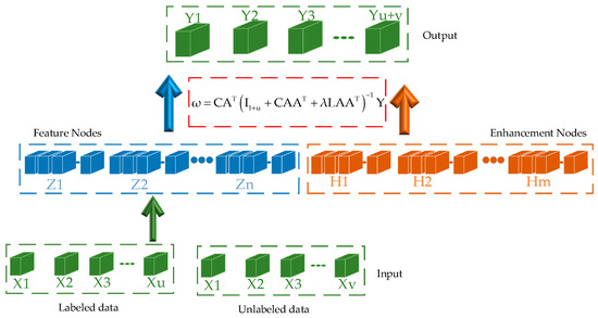
Figure 2.
SSBLS network operation principle diagram.
2.3. Regularized Correntropy Criterion (CC)
Since outliers can affect experimental results, the correlated entropy [28] is applied to solve such problems. If two arbitrary variables A and B are given, the relevant entropy expression is as follows:
where denotes the mathematical expectation, the Mercer kernel function, and a nonlinear function from the Hilbert space of functions. In this paper, the Gaussian kernel function is used, and its expression is as follows:
where represents the nuclear bandwidth. The correlation entropy loss function C-Loss is defined as follows:
The expression shows that the correlation entropy loss function is similar to the mean square error criterion, but the correlation entropy is in kernel space.
2.4. CC-SSBLS
Semi-supervised broad learning based on the mean square error criterion is not effective when encountering datasets containing large outliers. Therefore, a regularization-based correlation entropy criterion is introduced to replace the original calculation criterion. For the CC-SSBLS algorithm, the objective function is described as follows:
The Gaussian kernel on the correlation entropy is used, so the objective function can again be rewritten as follows:
To maximize Equation (10), the gradient descent method is used. Deriving from the above equation and then making it equal to 0 yields the following:
where is the Gaussian kernel, and denotes the amount of error associated with the ith training sample. By further organizing the above equation, it can be concluded that
To facilitate the representation, is used to denote . Therefore, the above equation is written in matrix form as follows:
Equation denotes the diagonal matrix, which can be expressed as . The structure diagram of the CC-SSBLS algorithm is shown in Figure 3. The pseudo code for the CC-SSBLS algorithm is shown in Algorithm 1.
| Algorithm 1: CC-SSBLS pseudo codes. |
| 1 Given |
| 2 A dataset with label , an unlabeled dataset , where ; |
| 3 The number of nodes per window of mapped features N1; |
| 4 The number of enhancement nodes N3, the activation function ; |
| 5 The regularization parameters and ; |
| 6 Bandwidth of the Gaussian kernel function ; |
7 Number of iterative windows N2;
|
| Else end. |
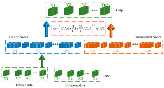
Figure 3.
CC-SSBLS network operation principle diagram.
3. Data and Experiments
3.1. Data
In recent years, the development and use of various clean energy sources have effectively alleviated the problem of air pollution. However, air pollution caused by vehicle emissions and various means of energy consumption in daily life remains a concern that people must address. The data for this paper were obtained from the China Meteorological Data website. Four cities in China, including Xuzhou, Nanjing, Beijing, and Changchun, were selected as the dataset to validate the effectiveness of the proposed model. The Beijing dataset was selected because Beijing is the capital of China, which can better reflect factors such as economic and geographical location. Similarly, Changchun, Jilin, is located in the north of China, which can better reflect the geographical location. The Nanjing and Xuzhou regions are located in the middle of China, and their economic and geographical location factors are the reasons for choosing the dataset in this region. These datasets span from 1 January 2018 to 31 December 2021, with data collected at one-hour intervals, and contain air pollutants as well as meteorological parameters. In this article, 80% of the dataset is the training set and 20% is the test set. The data information in the dataset is shown in Table 1 below, where T stands for temperature, H stands for dew point temperature, WS stands for wind direction, and WD stands for wind speed. The missing value and outlier information of the four datasets are described as follows: Missing values account for 70% of the Xuzhou dataset, and outlier information accounts for 40%. The experiments involved in this paper were all developed on the Python 3.9.7 platform. These experiments were conducted on a computer with a Win10 64-bit operating system running on an Intel Core (TM) i7-11800H @ 2.30 GHz with 16 GB of RAM.

Table 1.
Dataset partial data information.
3.2. Experimental Analysis
The BLS and SSBLS algorithms were compared to the CC-SSBLS method described in this section to show its efficacy, and the three algorithms were experimentally confirmed using the four datasets gathered. The dataset mentioned above was initially used to validate the BLS method. The experimental parameters were first established before the experiment’s start. The regularization coefficient c is 2−30, the number of nodes N3 of the augmentation layer is 300, and the number of windows N2 of the feature mapping layer is {5,6,7…,35}. The BLS algorithm processes the dataset’s data in three stages: first, the data are fed into the model, and the feature layer maps the data’s features; second, the augmentation layer adds nodes to the data; and third, the output data are solved pseudo inversely. We gather data for every iteration and use the final results to assess the efficacy of the model suggested in this research. We will use a number of evaluation measures to confirm the BLS algorithm’s performance. For this algorithm, its performance will be further verified through the following kinds of evaluation metrics: Root Mean Square Error (RMSE), Mean Absolute Error (MAE), Mean Absolute Percentage Error (MAPE), and R-square (R2), and their expressions are as follows:
where and denote the true and predicted values, respectively. The outcomes of the BLS algorithm’s evaluation metrics for each iteration window are displayed in Figure 4.
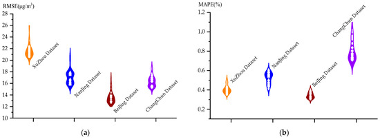
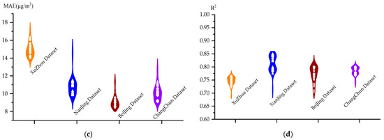
Figure 4.
Plot of metric results on the four datasets of the BLS algorithm: (a) RMSE, (b) MAPE, (c) MAE, and (d) R2.
The distribution of violins is depicted in the above figure. Each violin stands for the range of outcomes from the BLS model’s assessment metrics on a dataset, and by comparing each violin, one can determine the stability of the BLS model across all datasets. The evaluation metrics presented in Figure 4 demonstrate that the variation in the RMSE of the BLS algorithm on the four datasets is around 5 μg·m−3, the MAPE is approximately 0.4%, the MAE is approximately 4 μg·m−3, and the R2 is approximately 0.1. It is evident from the above results in the figure that the prediction effect is unstable and the BLS algorithm exhibits significant upward and downward variations on the four datasets. Based on the experimental findings, it is evident that out of all the iteration windows, the BLS algorithm performs optimally on the four datasets on windows 17, 12, and 17, during which the corresponding RMSEs are 20.61 μg·m−3, 15.76 μg·m−3, 12.67 μg·m−3, and 15.31 μg·m−3. It is evident from the findings of multiple evaluation indices that the BLS algorithm has a poor prediction effect. The prediction effect of the BLS algorithm for the Xuzhou dataset is displayed in Figure 5, which contains upper and lower sets of data graphs, with the upper set indicating the prediction curves for the whole dataset and the lower set indicating the localized prediction curves. This is achieved through the above experimental analysis, using the Xuzhou dataset as an example of air quality prediction at the optimal window.
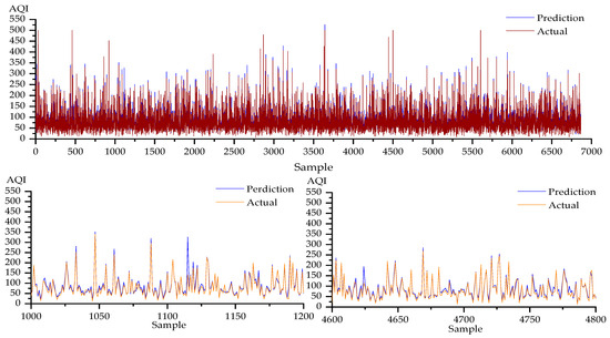
Figure 5.
Prediction results of the BLS algorithm on the Xuzhou dataset are plotted.
In the BLS prediction effect diagram, in order to better verify the prediction effect of the model, we selected 1000–1200 and 4600–4800 sample data for local verification. The BLS method produces inadequate prediction results on all four datasets, as shown in Figure 5, and there is a significant difference between the anticipated and actual values. We also included a semi-supervised approach to address the issues of low prediction accuracy and an unacceptable stability effect of the BLS algorithm due to missing values in the datasets. We first established the settings of the SSBLS algorithm before running trials with it. The feature mapping layer has a number of windows N2 of {5,6,7…,35}, the enhancement layer has a number of nodes N3 of 300, and the regularization parameter C is selected from {10−5,10−3,10−1,101,103,105}; through experimental analysis, C is set to 101 in this section; the weighting parameter λ is selected from {10−5,10−3,10−1,101,103,105}, and λ is set to 10−1 in this section. For every iteration, we gather data once, and the final data are used to assess the impact of the model that is suggested in this work. Comparably, the SSBLS algorithm is validated using four assessment metrics, and the resulting graph of the evaluation metrics is displayed in Figure 6.
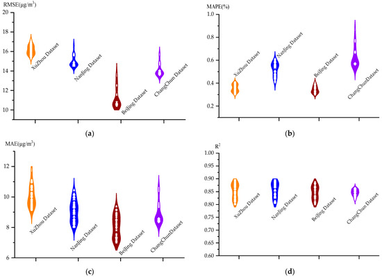
Figure 6.
Plot of metric results on the four datasets of the SSBLS algorithm: (a) RMSE, (b) MAPE, (c) MAE, and (d) R2.
As can be observed from the evaluation metrics in Figure 6, there is a difference of approximately 3 μg·m−3 between the up and down fluctuations of the RMSE of the SSBLS algorithm on the four datasets; the MAPE fluctuates up and down by approximately 0.3%; the MAE fluctuates up and down by approximately 3 μg·m−3; and the R2 fluctuates up and down by approximately 0.09. Compared to the BLS algorithm with the four datasets, the stability of the prediction results of the four assessment metrics of the SSBLS algorithm exhibited less upward and downward variation. The SSBLS algorithm performs optimally for the four datasets across all iteration windows at window numbers 31, 17, 17, and 17, where the RMSE values are 15.28 μg·m−3, 14.53 μg·m−3, 10.43 μg·m−3, and 13.64 μg·m−3. It can be seen from the results of several evaluation indicators that the prediction effect of the SSBLS algorithm is significantly improved compared with the BLS algorithm. When compared to the BLS algorithm, the SSBLS method successfully increases prediction accuracy and provides a more effective solution for missing data. Based on the experimental analysis above, Figure 7 illustrates the prediction effect of the SSBLS algorithm on the Xuzhou dataset. This dataset is used as an example of air quality prediction at the optimal window and consists of upper and lower sets of data graphs, where the upper set shows the prediction curves for the entire set of data and the lower set shows the prediction curves for the localized data.
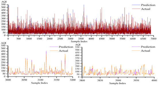
Figure 7.
Prediction results of the SSBLS algorithm for the Xuzhou dataset are plotted.
In the SSBLS prediction effect diagram, in order to better verify the prediction effect of the model, we selected 3000–3200 and 3800–4000 sample data for local verification. The results of Figure 7 demonstrate that the SSBLS algorithm performs better in terms of prediction on all four datasets, with a relatively small divergence between the expected and actual values. Additionally, the SSBLS approach performs better when addressing the issue of missing data. Processing the missing values in the datasets further improves the algorithm’s stability and prediction accuracy. To address the data outliers, the relevant entropy requirement is added to the SSBLS algorithm as the dataset we collected contains outlier information. An experimental investigation of the CC-SSBLS algorithm is presented below. Prior to confirming the CC-SSBLS algorithm’s efficacy, the pertinent algorithmic parameters were established. Of them, the weight parameter λ is selected from {10−5,10−3,10−1,101,103,105}, and λ is set to be 10−3 in this section through experimental analysis; the Gaussian kernel bandwidth σ is selected from {1,3,5,7,9}, and σ is set to 1 through experimental analysis in this section. Furthermore, the regularization parameter C is chosen from {10−5,10−3,10−1,101,103,105}, and C is set to be 101 in this section through experimental analysis. The following aspects will be separated into the steps of this experiment: Initially, the gathered dataset will be fed into the feature mapping model, and concurrently, the number of nodes in each window of the mapping layer will be adjusted in the feature mapping process (N1); subsequently, the enhancement nodes will be added, with the number of enhancement nodes being set to 300 in the experiments; finally, the output layer of the model will be fed with the results of both the mapping and enhancement layers. Subsequently, the output layer of the network receives the inputs from the mapping and enhancement layers. The pseudo-inverse is solved using the correlation entropy criterion rather than the mean square error criterion to produce the final output. {5,6,7,…,35} is the number of iteration windows (N2) of the algorithm. We gather data for every iteration, and the final data are what we use to assess how effective the model this paper proposes is. The outcomes of the CC-SSBLS algorithm’s evaluation metrics on the Xuzhou dataset, using it as an example, are displayed in Figure 8 below.
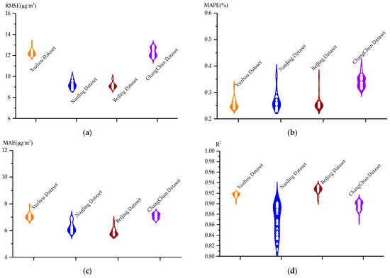
Figure 8.
Plot of metrics results on the four datasets of the CC-SSBLS algorithm: (a) RMSE, (b) MAPE, (c) MAE, and (d) R2.
Figure 8 shows that the RMSE of the CC-SSBLS method for the four datasets has an up-and-down difference of about 2 μg·m−3, the MAPE has an up-and-down difference of approximately 0.1%, the MAE has an up-and-down difference of approximately 2 μg·m−3, and the R2 has an up-and-down difference of approximately 0.08. The upward and downward fluctuations of the evaluation indexes of the CC-SSBLS algorithm for the four datasets are further reduced compared to the SSBLS algorithm, and the stability of the prediction results is further improved. The best results are obtained with the CC-SSBLS method for the four datasets at iteration windows 18, 18, 20, and 35, where the RMSEs are 11.94 μg·m−3, 8.68 μg·m−3, 8.75 μg·m−3, and 11.73 μg·m−3, respectively. From the results of several evaluation indicators, it is obvious that the prediction effect of CC-SSBLS algorithm is better than that of the SSBLS algorithm. Figure 9 illustrates the prediction effect of the CC-SSBLS algorithm for the four datasets for air quality prediction at the optimal window through the above experimental analysis, using the Xuzhou dataset as an example. The upper and lower sets of data graphs show the prediction curves for the entire dataset, while the lower set shows the localized prediction curves.
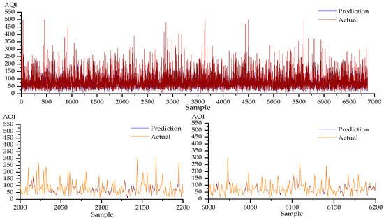
Figure 9.
Prediction results of the CC-SSBLS algorithm on the Xuzhou dataset are plotted.
In the prediction effect diagram for the CC-SSBLS algorithm, in order to better verify the prediction effect of this model, we selected 2000–2200 and 6000–6200 sample data for local verification. The CC-SSBLS method has a better prediction effect for the four datasets, as shown in Figure 9, and there is not a noticeable difference between the anticipated and actual values. The CC-SSBLS algorithm predicts air quality more accurately than the BLS and SSBLS algorithms together. After a thorough analysis of the three algorithms mentioned above, it can be concluded that the CC-SSBLS algorithm has a better prediction effect and has more stable prediction impact during iteration than the BLS and SSBLS algorithms. Table 2 displays the three methods’ parameter configurations for the four datasets.
Table 2.
Parameter settings for BLS, SSBLS, and CC-SSBLS.
Table 3 shows that the N3 of BLS, SSBLS, and CC-SSBLS are consistent. Based on this, we primarily alter the N1 and N2 parameters during the experiment to maximize the prediction effect of the algorithm. Figure 10 displays a comparison chart of the best evaluation indexes for the three algorithms based on the findings of our experimental investigation of the evaluation indexes of the three algorithms on the four datasets.
Table 3.
Comparison of evaluation indicators for several models.
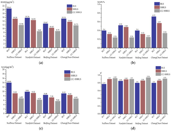
Figure 10.
Optimal evaluation metric values for the three algorithms on the four datasets. (a) Graph representing the RMSE optima of the three algorithms on the four datasets. (b) Graph representing the MAPE optima of the three algorithms on the four datasets. (c) Graph representing the MAE optima of the three algorithms on the four datasets. (d) Graph representing the R2 optima of the three algorithms on the four datasets.
As seen in Figure 10, the three algorithms BLS, SSBLS, and SSBLS exhibit decreasing trends for the four datasets for RMSE. They also exhibit decreasing trends for MAPE and MAE, and they exhibit increasing trends for R2. The CC-SSBLS model outperforms the other two models in every assessment index shown in the picture, showing superior fitting and prediction abilities. Therefore, it can be inferred that the CC-SSBLS model has a superior prediction effect and a more stable prediction result by examining the variations in the values of the evaluation index results of the three models stated above.
3.3. Results and Analysis
We carried out comparative tests to better illustrate the prediction effect of the CC-SSBLS model. As we discovered in the previous part, the CC-SSBLS model has a greater prediction effect than the BLS and SSBLS models. For this reason, we compare the CC-SSBLS model with the prediction models from the RF, V-SVR, BLS, SSBLS, ANN, and RNN methods in this section. In order to reflect the prediction effect of different models on AQI, in this section, we use four datasets to conduct experimental verification of several models. The comparison result plots of multiple models are displayed in Figure 11, Figure 12, Figure 13 and Figure 14, and each plot comprises upper and lower sets of data plots, where the upper set represents the prediction curves for all the data, and the lower set represents the local prediction curves.
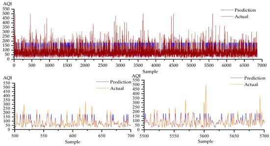
Figure 11.
Prediction results of the RF algorithm on the Xuzhou dataset are plotted.
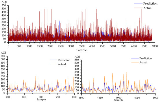
Figure 12.
Prediction results of the V-SVR algorithm on the Nanjing dataset are plotted.
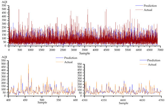
Figure 13.
Prediction results of the ANN algorithm on the Beijing dataset are plotted.
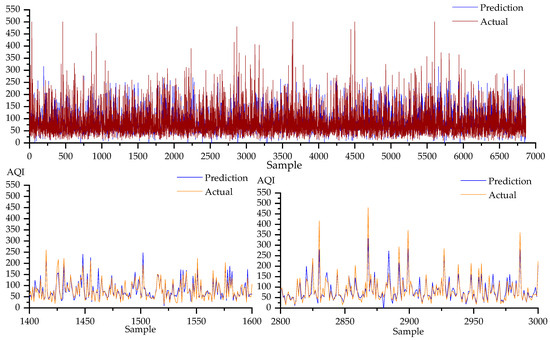
Figure 14.
Prediction results of the RNN algorithm on the Changchun dataset are plotted.
In contrast to the RF, V-SVR, BLS, SSBLS, ANN, and RNN models, the CC-SSBLS model has the best prediction impact for the dataset, as shown by a comparison of the prediction effect graphs in Figure 5, Figure 7, Figure 9, Figure 11, Figure 12, Figure 13 and Figure 14. All of the models mentioned above have been compiled and analyzed, and Table 3 below displays the findings of each model’s evaluation index.
Using the Xuzhou dataset as an example, it can be seen from the table that the CC-SSBLS model value for RMSE is 11.94 μg·m−3, which is the lowest value among multiple models and 3.31 μg·m−3 less than that of SSBLS. The CC-SSBLS model value for MAE is 6.89 μg·m−3, the lowest of various models and 2.30 μg·m−3 less than that of SSBLS. The CC-SSBLS model for MAPE had a value of 0.24%, the lowest of multiple models and 0.08% less than SSBLS. The greatest value among several models for R2 is 0.92 for the CC-SSBLS model, which is 0.02 more than the value for SSBLS. Thus, the CC-SSBLS model outperforms multiple alternative models for each assessment criteria. In the same way, the CC-SSBLS model performs better than the other models for the following three datasets.
4. Conclusions
Outliers in the data are discovered to result in less-than-ideal model predictions when air quality prediction is performed. Considering that correlation entropy is more effective in addressing the issue of data outliers, the predictive air quality model CC-SSBLS is suggested. The model modifies the pseudo-inverse solution technique and substitutes the correlation entropy criterion for the mean square error criterion in the broad learning system. The experimental findings validate the efficacy of the model.
The following summary applies to the CC-SSBLS model proposed in this paper:
- (1)
- Through validation on the four datasets gathered for this paper, it is demonstrated that the correlation entropy criteria performs better when handling dataset outliers. In terms of predictive efficacy, the CC-SSBLS model performs better than the CART-SSBLS model and a number of other comparison models that are discussed above;
- (2)
- The efficacy of the model is validated by using the four datasets gathered in this study for validation. These datasets demonstrate that the stability of the prediction results of CC-SSBLS is superior to that of BLS;
- (3)
- For the model in this paper, only the prediction effect for the data is analyzed in detail, but the time analysis of model training is ignored. At a later stage, the training time of the model can be further studied to reduce the time consumed by the training model and improve the efficiency of the model.
- (4)
- As for the prediction effect for the AQI, the broad learning system should be further studied in the future to further strengthen the prediction effect. For the broad learning system, subsequent studies can be conducted on many aspects, such as the feature layer, the enhancement layer and the pseudo-inverse solving principle, so as to further improve the prediction effect of the model, reduce the training time and improve the prediction efficiency of the model.
Author Contributions
Conceptualization, L.W. and Y.W.; methodology, L.W.; software, L.W. and Y.W.; validation, Y.W.; formal analysis, Y.W.; investigation, L.W. and Y.W.; resources, L.W.; data curation, L.W.; writing—original draft preparation, Y.W.; writing—review and editing, L.W. and Y.W.; supervision, L.W.; project administration, L.W., S.Z., L.Z. and J.C.; funding acquisition, Y.W. All authors have read and agreed to the published version of the manuscript.
Funding
This research received no external funding.
Institutional Review Board Statement
Not applicable.
Informed Consent Statement
Not applicable.
Data Availability Statement
The datasets of the current study are available from the corresponding author on reasonable request. The data are not publicly available due to privacy.
Conflicts of Interest
The authors declare no conflicts of interest.
References
- Habibi, R.; Alesheikh, A.A.; Mohammadinia, A.; Sharif, M. An Assessment of Spatial Pattern Characterization of Air Pollution: A Case Study of CO and PM2.5 in Tehran, Iran. ISPRS Int. J. Geo-Inf. 2017, 6, 270. [Google Scholar] [CrossRef]
- Deters, J.K.; Zalakeviciute, R.; Gonzalez, M. Modeling PM2.5 Urban Pollution Using Machine Learning and Selected Meteorological Parameters. J. Electr. Comput. Eng. 2017, 2017, 5106045. [Google Scholar]
- Huang, K.; Xiao, Q.; Meng, X. Predicting monthly high-resolution PM2.5 concentrations with random forest model in the North China Plain. Environ. Pollut. 2018, 242, 675–683. [Google Scholar] [CrossRef]
- Chen, G.; Li, S.; Knibbs, L.D.; Hamm, N.A.; Cao, W.; Li, T.; Guo, J.; Ren, H.; Abramson, M.J.; Guo, Y. A machine learning method to estimate PM2.5 concentrations across China with remote sensing, meteorological and land use information. Sci. Total Environ. 2018, 636, 52–60. [Google Scholar] [CrossRef] [PubMed]
- Wang, Y.J.; Jiang, S.; Huang, L.; Lu, G.; Kasemsan, M.; Yaluk, E.A. Differences between VOCs and NOx transport contributions, their impacts on O3, and implications for O3 pollution mitigation based on CMAQ simulation over the Yangtze River Delta, China. Sci. Total Environ. 2023, 872, 2118–2120. [Google Scholar] [CrossRef] [PubMed]
- Di, G.L.; Lapucci, M.; Schoen, F. Improved Maximum Likelihood Estimation of ARMA Models. Lobachevskii J. Math. 2022, 43, 2433–2443. [Google Scholar]
- Tarmanini, C.; Sarma, N.; Gezegin, C. Short term load forecasting based on ARIMA and ANN approaches. Energy Rep. 2023, 9, 550–557. [Google Scholar] [CrossRef]
- Kożuch, A.; Cywicka, D.; Adamowicz, K. A Comparison of Artificial Neural Network and Time Series Models for Timber Price Forecasting. Forests 2023, 14, 177. [Google Scholar] [CrossRef]
- Peng, S.J.; Shen, J.; Chao, Z.X. PM2.5 prediction based on ARIMA model. Saf. Environ. Eng. 2014, 21, 125–128. [Google Scholar]
- Zhang, L.Y.; Qiu, R.Z.; Hu, X.S. Trend analysis and forecast of PM2.5 in Fuzhou, China using the ARIMA model. Ecol. Indic. 2018, 95, 702–710. [Google Scholar] [CrossRef]
- Hu, J.L.; Chen, J.J.; Ying, Q. One-year simulation of ozone and particulate matter in China using WRF/CMAQ modeling system. Atmos. Chem. Phys. 2016, 16, 10333–10350. [Google Scholar] [CrossRef]
- Liang, Y.C.; Maimury, Y. Machine Learning-Based Prediction of Air Quality. Appl. Sci. 2020, 10, 9151. [Google Scholar] [CrossRef]
- Ghaemi, Z.; Alimohammadi, A.; Farnaghi, M. LaSVM-based big data learning system for dynamic prediction of air pollution in Tehran. Environ. Monit. Assess. Int. J. 2018, 190, 300. [Google Scholar] [CrossRef] [PubMed]
- Liu, H.; Li, Q.; Yu, D.; Gu, Y. Air Quality Index and Air Pollutant Concentration Prediction Based on Machine Learning Algorithms. Appl. Sci. 2019, 9, 4069. [Google Scholar] [CrossRef]
- Zhang, J.; Ding, W. Prediction of air pollutants concentration based on an extreme learning machine: The case of Hong Kong. Int. J. Environ. Res. Public Health 2017, 14, 114. [Google Scholar] [CrossRef] [PubMed]
- Jiang, F.; He, J.Q.; Tian, T.H. A clustering-based ensemble approach with improved pigeon-inspired optimization and extreme learning machine for air quality prediction. Appl. Soft Comput. 2019, 85, 105827. [Google Scholar] [CrossRef]
- Qiao, D.W.; Yao, J.; Zhang, J.W. Short-term air quality forecasting model based on hybrid RF-IACA-BPNN algorithm. Environ. Sci. Pollut. Res. 2022, 29, 39164–39181. [Google Scholar] [CrossRef]
- Feng, R.; Zheng, H.J.; Gao, H. Recurrent Neural Network and random forest for analysis and accurate forecast of atmospheric pollutants: A case study in Hangzhou, China. J. Clean. Prod. 2019, 231, 1005–1015. [Google Scholar] [CrossRef]
- Belavadi, S.V.; Rajagopal, S. Air Quality Forecasting using LSTM RNN and Wireless Sensor Networks. Procedia Comput. Sci. 2020, 170, 241–248. [Google Scholar] [CrossRef]
- Zhang, Z.D.; Zeng, Y.K.; Yan, K. A hybrid deep learning technology for PM2.5 air quality forecasting. Environ. Sci. Pollut. Res. 2021, 28, 39409–39422. [Google Scholar] [CrossRef]
- Qin, D.; Yu, J.; Zou, G. A novel combined prediction scheme based on CNN and LSTM for urban PM2.5 concentration. IEEE Access 2019, 7, 20050–20059. [Google Scholar] [CrossRef]
- Wu, Z.Y.; Wang, Y.; Zhang, L. MSSTN: Multi-scale spatial temporal network for air pollution prediction. IEEE Int. Conf. Big Data 2019, 12, 1547–1556. [Google Scholar]
- Han, J.D.; Liu, H.; Zhu, H.S. Joint air quality and weather prediction based on multi-adversarial spatiotemporal networks. arXiv 2021, arXiv:2012.15037. [Google Scholar] [CrossRef]
- Chen, C.; Liu, Z. Broad Learning System: An Effective and Efficient Incremental Learning System Without the Need for Deep Architecture. IEEE Trans. Neural Netw. Learn. Syst. 2018, 29, 10–24. [Google Scholar] [CrossRef] [PubMed]
- Liu, Z.; Zhou, J.; Chen, C.L.P. Broad learning system: Feature extraction based on K-means clustering algorithm. Int. Conf. Inf. 2017, 4, 683–687. [Google Scholar]
- Wang, L.; Wang, Y.B.; Chen, J. A PM2.5 Concentration Prediction Model Based on CART–BLS. Atmosphere 2022, 13, 1674. [Google Scholar] [CrossRef]
- Pourmir, M.R.; Monsefi, R.; Hodtani, G.A. Signal Detection in MIMO Communications System with Non-Gaussian Noises based on Deep Learning and Maximum Correntropy Criterion. Int. J. Wirel. Mob. Netw. 2022, 14, 1–16. [Google Scholar] [CrossRef]
- Yang, J.; Cao, J.W.; Wang, T.L. Regularized correntropy criterion based semi-supervised ELM. Neural Netw. 2020, 122, 117–129. [Google Scholar] [CrossRef]
- Huang, G.; Song, S.; Wu, C. Semi-supervised and unsupervised extreme learning machines. IEEE Trans. Cubernetics 2017, 44, 2405–2417. [Google Scholar] [CrossRef]
Disclaimer/Publisher’s Note: The statements, opinions and data contained in all publications are solely those of the individual author(s) and contributor(s) and not of MDPI and/or the editor(s). MDPI and/or the editor(s) disclaim responsibility for any injury to people or property resulting from any ideas, methods, instructions or products referred to in the content. |
© 2024 by the authors. Licensee MDPI, Basel, Switzerland. This article is an open access article distributed under the terms and conditions of the Creative Commons Attribution (CC BY) license (https://creativecommons.org/licenses/by/4.0/).