Abstract
With China’s rapid industrialization and urbanization in the process of socio-economic development, the extensive use of energy has resulted in a large amount of CO2 emissions, which puts great pressure on China’s carbon emission reduction task. Through multivariate socio-economic data, this paper proposes an extraction and screening method of multivariate variables based on land-use types, and the downscaled spatial decomposition of carbon emissions at different scales was carried out by using the spatial lag model (SLM). This paper makes up for the shortcomings of previous studies, such as an insufficient modeling scale, simple modeling variables, limited spatio-temporal span of spatial decomposition, and no consideration of geographical correlation. Based on the results of the spatial decomposition of carbon emissions, this paper explores the spatial and temporal dynamics of carbon emissions at different scales. The results showed that SLM is capable of downscaling the spatialization of carbon emissions with high precision, and the continuity of the decomposition results at the provincial scale is stronger, while the differences of the decomposition results at the municipal scale are more obvious within the municipal units. In terms of the spatial and temporal dynamics of CO2 emissions, carbon emissions at both scales showed a significant positive correlation. The dominant spatial correlation types are “Low–Low” at the provincial level, and “Low–Low” and “High–High” at the municipal level. The smaller spatial scope is more helpful to show the geographic dependence and geographic differences of China’s carbon emissions. The findings of this paper will help deepen the understanding of the spatial and temporal changes of carbon emissions in China. They will provide a scientific basis for the formulation of feasible carbon emission reduction policies.
1. Introduction
Since the twentieth century, anthropogenic carbon emissions have accounted for more than 99 per cent of all carbon emissions [1], and the term “carbon emissions” is used herein to refer to anthropogenic carbon emissions. According to the United Nations Intergovernmental Panel on Climate Change (IPCC), the main cause of global warming is the increase in the CO2 concentration in the atmosphere, and the main reason for the increase in the CO2 concentration is fossil energy consumption [2,3]. Carbon emissions are related to the core interests of each country and have become the focus of international attention [4]. With the continuous development and progress of China’s economy and society, China’s energy consumption and carbon emissions have increased dramatically [5,6]. Although China has not yet been included in the list of the first batch of countries limited to an emission reduction under the Kyoto Protocol, the changes in China’s carbon emissions have attracted the attention of various countries. Due to the vastness of China’s territory and the uneven level of regional economic development, there are large regional differences in carbon emissions. China’s government has a positive attitude in dealing with carbon emission reduction, and only by grasping the spatial and temporal distribution of carbon emissions can governments formulate policies for different regions [2].
In foreign studies on the spatial decomposition and spatial-temporal dynamics of carbon emissions, Chevallier et al. decomposed carbon emissions on a globally uniform grid [7]. However, the modeling scale of the study was the national scale, which is not fine enough. Some studies have developed carbon emission maps based on nighttime lighting data [1]. However, nighttime lighting data do not accurately cover anthropogenic areas [8]. The spatial estimation of carbon emissions using only a single variable, such as nighttime lighting, is a single variable system, and it is not possible to take multiple factors into account more comprehensively in order to make a more accurate spatial prediction of carbon emissions. In the domestic exploration of carbon emissions, some studies have examined the distribution of CO2 emissions in multiple cities or regions. For example, Wang et al. estimated CO2 based on nighttime lighting data and obtained the CO2 distribution of cities in the Yangtze River Delta [9]. However, carbon emissions are sensitive to scale changes, and the findings of CO2 emission distribution in a specific region are not suitable to be transferred to another spatial scale [10]. Therefore, large-scale spatial studies of carbon emissions are still necessary for government policy makers [11]. Even though some scholars have conducted gridded studies of carbon emissions on a large scale, the models they use cannot take the spatial linkage of carbon emissions into account [12]. At present, the modeling regression scales for downscaling the spatialization of carbon emissions in China are basically carried out at the provincial scale, and no attempt has been made to carry out spatial decomposition at the more detailed municipal scale [13]. In addition, the large-scale long-term time-series CO2 distribution has still not been adequately studied in recent years, and needs to be explored with improved methods and indicators to effectively understand the spatial and temporal dynamics of socio-environmental problems [14].
In order to realize an effective understanding and control of China’s domestic carbon emissions, and to realize a detailed quantification of carbon emissions in time and space, this paper carries out the downscaling spatial decomposition of carbon emissions based on multivariate spatial statistics, applying SLM at the provincial and municipal scales in China, and investigates its spatial-temporal distribution law at the two scales. This helps to grasp the distribution characteristics and regional differences of carbon emissions in China, and provides a reference for the formulation of reasonable regional carbon emission reduction policies. The research flow chart is shown in Figure 1.
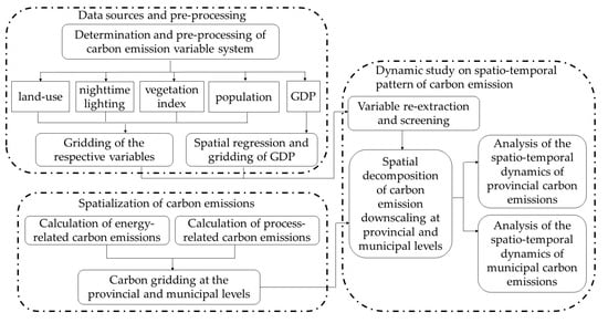
Figure 1.
The research flow chart.
2. Data and Methods
2.1. Study Area
China is a vast country, but due to natural, historical, and social factors, the level of economic development within the region is not balanced, and CO2 emissions are significant and unevenly distributed [13]. In this study, mainland China was taken as the study area, and Hong Kong, Macao, Taiwan, and Tibet were not included due to the lack of statistical data. Multiscale spatial and temporal dynamics were analyzed at the 1 km pixel scale for the administrative levels of provinces and cities. The term “city” here refers to the administrative prefecture-level city, not the built-up city, which is the same as below.
2.2. Data Sources and Pre-Processing
Land-use data (land-use) and vegetation index data (NDVI) were obtained from the Land Processing Distributed Active Archive Center (LP DAAC) (https://lpdaac.usgs.gov/products/ (accessed on 3 October 2022)). The agency operates as a partnership between the U.S. Geological Survey (USGS) and the National Aeronautics and Space Administration (NASA). Land Cover Type MCD12Q1 Version 6.1 data were improved by making a variety of calibration changes, including changes to the scanning angle (RVS) method and correcting for crosstalk in the TerraMODIS infrared band. The specific categorization of this dataset can be found in the summary of Zhang et al. [15].
Population data were selected from Oak Ridge National Laboratory (ORNL) LandScan Global data (https://landscan.ornl.gov/ (accessed on 16 March 2023)). LandScan Global uses an innovative approach to population modeling that combines geospatial science, remote sensing technology, and machine learning algorithms. LandScan Global captures the full range of potential spaces for people to move around in during the day and night, not just residential locations.
Nighttime lighting data (NPP-VIIRS) were derived from NOAA/NGDC (https://payneinstitute.mines.edu/eog/nighttime-lights/ (accessed on 11 June 2022)). The NOAA/NGDC observing team utilized nighttime data acquired by the Visible Infrared Radiometer (VIIRS) aboard the National Polar Cooperation Satellite (Suomi-NPP) to obtain the first version of a composite image dataset of average monthly radiation. The annual VNL V1 version excludes data on the effects of stray light [16], but does not filter out effects from auroras, fires, fishing boat lights, and other ephemeral light sources. A new annual VIIRS nighttime light time series, VNL V2, was generated from monthly cloud-free mean radiation data [17]. The VNL V2 version of the file discards high emissivity and low emissivity anomalies and filters out most fires. Therefore, the annual VNL V2 version of the file was used in this paper as remote sensing data for nighttime lighting.
GDP data were obtained from China Economic and Social Development Statistics Database—Yearbook Navigator (https://data.cnki.net/home (accessed on 1 April 2023)). The database integrates various types of statistical information, applies knowledge graphs, models, and other artificial intelligence techniques to upgrade it, and completes the structured and indexed organization of data. Administrative boundaries data were obtained from the National Center for Basic Geographic Information (http://www.ngcc.cn/ (accessed on 6 April 2022)).
Provincial energy consumption data [18,19,20,21] and municipal carbon emissions data [22,23,24,25] were obtained from China Carbon Accounting Databases (CEADs) (https://www.ceads.net/ (accessed on 10 November 2022)). CEADs is committed to building a cross-checkable multiscale carbon emission accounting methodology system, compiling a carbon accounting inventory covering China and other developing economies, and building a refined carbon accounting data platform.
For the processing of the night light data, the average radiation value originating from the unoccupied area closest to the dense human settlements—the average radiation value within Lake Taihu—was selected as a low threshold to remove the noise in this paper [13,26]. In the removal step, a binary raster file for the intermediate step was first generated according to Equation (1).
where DN(n,i) represents the i-th raster in year n and DN(n,t) represents the threshold in year n.
Afterwards, the binary raster was multiplied with the original raster to obtain the NPP-VIIRS data with low-value noise removed. In order to standardize the scale of all variable data, NPP-VIIRS, land-use data, NDVI, and population data were resampled with an image size of 1 km2 in this paper. In addition, NDVI data required null removal and scale reduction.
2.3. Pre-Processing of GDP
NPP-VIIRS has been shown to have better performance in GDP downscaling than DMSP/OLS data [27,28]. However, some scholars have found that NTLs on different land-use types are not comparable and cannot be simply used to fit GDP, and choosing a single indicator is likely to cause problems such as poor fitting accuracy [29]. Therefore, in this paper, NPP-VIIRS was used for three indicators under different land-use types, and the calculation process is shown in Equation (2) [30].
where DNj denotes the sum of NTL lights of n pixels on land class j, Land Area (YLj) and Land Area (NLj) are the lighted and unlighted areas on land class j, LandYL and LandNL denote the lighted and unlighted areas in the city’s administrative boundaries, and Pj denotes the weight of the area occupied by land class j in the city. The sum of the weights is 100% (valid land classes).
After that, this paper carried out multiple linear stepwise regression based on the statistical indicators, and the regression model is shown in Equation (3). After the multivariate stepwise regression, the R2 reached 0.9, which proved that the application of the multivariate stepwise regression model to the NPP-VIIRS index based on land category could better spatially decompose the GDP. Based on the model fitting results, this paper spatially decomposed GDP on a raster scale, and obtained the gridded GDP 1 km × 1 km data for each year from 2012 to 2021. See Supplementary Materials Figure S1 for gridded GDP for 2012 and 2021 as an example.
where Y is the dependent variable, that is, the regression value (fitting value) of GDP; Xi (i = 1, 2, …, n) is the independent variable; and βi is the regression coefficient of Xi.
2.4. Spatialization of Carbon Emissions
2.4.1. Carbon Emission Statistics and Screening of Variables
In this paper, carbon emission statistics for 30 provincial-level administrative regions were calculated with reference to the calculation process of IPCC and CEADs. Two components make up the emission statistics: energy-related emissions due to fossil fuel combustion (CEenergy-related,j), and process-related emissions due to industrial production (CEprocess-related,j) [25]. The calculation process is described in Equation (4). The process of calculating CEenergy-related,j based on mass balance theory is described in Equation (5) [23,24], and the steps for calculating CEprocess-related,j are described in Equation (6) [18,19,22]:
where ADij is the fossil fuel consumption of fossil fuel I in sector j. NCVi, CCi, and Oij represent the emission factors of the fuels burned in sector j, respectively, and can be further divided into three components: the net calorific value of the fuel NCVi, which is formed per physical unit of fossil fuel i burned; the carbon content CCi, which is produced per unit of calorific value of fossil fuel i burned; and the fossil fuel oxidation rate Oij. Specific values are given in the collation of Shan et al. [20,25].
where ADt,j and EFt,j are industrial production activity data and emission factors respectively, where EFt,j value is 0.4985 [25].
In terms of the selection of the independent variables for carbon emissions, there are numerous factors that influence carbon emissions. The spatialization of downscaling of carbon emissions needs to take into account as many factors as possible, taking into account the availability of data and the need for easy quantification and spatialization [31,32]. Since the socio-economic data on different land-use types are not comparable, choosing a single indicator to fit the dependent variable is likely to cause problems such as lower fitting accuracy [29]. Therefore, this paper considered the following multiple independent variables for the spatial decomposition of carbon emissions.
Nighttime lighting data have the advantages of wide coverage, long time span, and large area for simultaneous acquisition of ground information [33]. They can reveal the intensity of economic and human activities and have become one of the most important geographic information data [34,35]. A correlation between nighttime lighting data and carbon emissions has been demonstrated and can be used to measure carbon emissions [33]. Most of the previous studies were measured using DMSP-OLS nighttime lighting data, which stopped being updated after 2013 [36]. The NPP-VIIRS nighttime light data not only fill the data gap after 2013, but also have higher spatial resolution and are more suitable for near-term studies.
Vegetation, as a major CO2 absorber, is also strongly correlated with carbon emissions. Remote sensing has become increasingly important in the study of surface vegetation cover over the past few decades as an important means of assessing changes in vegetation cover [37]. Based on the differences in the response of vegetation to the spectral features of different bands, the vegetation index indicating the surface vegetation can be obtained through the calculation of different bands [38]. NDVI is very sensitive to the growth potential of green vegetation and can be used for regional vegetation cover studies.
As the urban population gathers, environmental problems related to air pollution and energy consumption will emerge [39]. The impact of population distribution on CO2 emissions in China is significant [40]. Unlike population density measurements such as WorldPop, LandScan data are census data measured based on GIS and a density difference model. The model takes into account all urban economic activity [41]. The LandScan population database estimates economic activity per square kilometer in the form of raster element values. This overcomes biases in the measurement of urban demographics and provides a more accurate and scientific picture of the spatial distribution of the population [42].
Considering the above reasons, this paper was based on NPP-VIIRS and NDVI data for extraction and statistics on different land classes for a more complete and comprehensive variable screening. Since population data and GDP are not directly measured but are quadratic fitted values, splitting them may affect the accuracy of their data and therefore these two types of data were not split. Next, all variables were factor analyzed to examine the main components of the variables. Then, based on the results of the factor analysis, the variables were subjected to recombination extraction and correlation analysis as a way to carry out the initial screening of the independent variables. After obtaining the preliminary screening variables, this paper carried out in-depth screening of independent variables based on causality method, random forest analysis, stepwise regression, Lasso regression, ridge regression, elastic network screening, and optimal subset screening method.
2.4.2. Spatial Regression of Carbon Emissions
In spatial distribution, the dependent variable on a certain geographic unit is not only related to the socio-economic data, but is also affected by the dependent variables of its neighboring geographic units; therefore, this paper adopted the spatial regression analysis model to explore the spatial dynamics of carbon emissions in China. Spatial lag modeling (SLM) is used to represent spatial correlation and can reflect the impact of neighboring regions on the target region. Therefore, this paper selected SLM for spatial regression to calculate the fitted carbon emission values for each grid, based on the grid layer storing the carbon emissions and the screened independent variables. The model equation is shown in Equation (7):
where Wy is the spatial weight matrix; ρ denotes the regression coefficient of Wy; x1 to xi denote the values of the independent variables influencing factors; β1 to βi denote the regression coefficients of the respective variables; and ε is the random error.
In this paper, the negative grid value in the fitting result was set to a value of 0, which is closest to the negative value among the possible values [12], so that the preliminary carbon emission fitting grid layer could be obtained. After that, this paper adopted the correction method of making the sum of the fitted values of the administrative units consistent with the real value of carbon emissions, so that the error only occurred within each administrative unit [12], and the specific adjustment process is shown in Equation (8):
where CC is the final adjusted value of carbon emissions, SC is the real value of carbon emissions, NC is the preliminary estimated value, c is each image element, n is each administrative unit under a certain scale, and t is each year.
2.4.3. Study of the Dynamics of Spatial and Temporal Patterns
The coefficient of variation (CV) can reflect the degree of agglomeration or dispersion of a parameter to a certain extent. Therefore, this paper adopted the CV to calculate and explore the spatial distribution of carbon emissions at different scales in China, and the calculation is shown in Equation (9):
where CV represents the coefficient of variation, the value of which corresponds to the degree of agglomeration of the samples within a certain range and is positively correlated with the intensity of agglomeration; Yi represents the value of carbon emissions within area I; n represents the number of administrative units; and is the average carbon emissions. According to the existing research results, if the coefficient of variation CV is greater than 0.2, the variation between observations is significant [43].
When exploring changes in carbon emissions in different provinces and cities, it is necessary to determine whether a given unit is spatially autocorrelated within the study area [44]. Global Moran’s I reveals similarities between the attribute values of connected or neighboring geographic units as a basis for assessing the spatial distribution across the study area [45]. Therefore, in this paper, global Moran’s I was utilized to measure and assess the overall autocorrelation of carbon emissions at various scales, as calculated in Equation (10).
where I denotes the global Moran’s I index; n is the total number of administrative districts at a given scale; i and j are two different administrative districts at the same scale; wij is the spatial weighting matrix; xi and xj are the simulated CO2 emissions of provinces i and j, respectively; and is the average emission of the entire study area.
Local spatial autocorrelation analysis can determine to what extent the overall autocorrelation masks the uncertainty of the local distribution [46]. LISA can assess the degree of spatial correlation between the eigenvalues of a regional unit and the environment in which it is located [12,47]. Therefore, in this paper, Moran scatterplot and LISA data were combined to study the spatial aggregation and regional instability of carbon emissions at various scales. The local Moran’s I index in LISA is calculated as shown in Equation (11):
where Ii denotes the local Moran’s I index, zi and zj are normalized to the sample values of regions i and j, and wij refers to the spatial weights, where = 1.
3. Results and Discussion
3.1. Screening of Carbon Emission Variables
In this paper, based on the rotated principal component analysis table that can be seen in Supplementary Materials Table S1, the land classes that contributed more to the principal components were merged into the following five: L1—forestland, L2—grassland, L3—farmland, L4—urban, and L5—water (Supplementary Materials Table S2). The NPP-VIIRS and NDVI were counted based on the merged land classes. Then, they were combined with four summation indicators: Sum-NPP-VIIRS, Sum-NDVI, Sum-GDP, and SUM-population for the correlation analysis (Supplementary Materials Table S3). Among them, the VIFs of SUM-NPP-VIIRS and NPP-VIIRS-13 reached approximately 30, and it was necessary to make a trade-off between these two variables. Considering that SUM-NPP-VIIRS contains more comprehensive data information compared to NPP-VIIRS-13, SUM-NPP-VIIRS of the two was selected to be retained as a candidate independent variable.
In the screening of multivariate independent variables, it is necessary to follow the causality network method first: independent variables can be included in the independent variable system only when there is a theoretical logical correlation between independent variables and the dependent variables. As shown in Table 1, the screening results of the optimal subset method all have a logical causal relationship with anthropogenic carbon emissions, so this paper chose the results of the optimal subset method: SUM-GDP, SUM-NDVI, SUM-NPP-VIIRS, NDVI-L1, NDVI-L3, NDVI-L4, NPP-VIIRS-L1, and NPP-VIIRS-L2. These eight variables were used as independent variables that eventually entered the spatial regression model of carbon emissions.

Table 1.
Screening variable results for multiple methods.
3.2. Spatial Regression of Carbon Emissions
The results of the spatial analysis of the SLM of carbon emissions are shown in Table 2. The provincial model fit goodness of fit R2 all reached above 0.633, while the municipal level was approximately 0.990. These data confirm the higher fit of the model for carbon emissions. The reason that the R2 of the regression at the municipal level was higher than that at the provincial level is that the area with the same value of the preliminary allocation of carbon emission grid value at the provincial level was larger, resulting in a weaker difference in spatial pattern than that at the municipal level. The regression coefficient of the spatially lagged variable W_carbon reveals the inherent correlation, and the reason for the difference in W_carbon at the two scales is the same as for the R2 value. It can be seen that the values of W_carbon in the provincial regressions are all greater than or equal to 0.740, and the W_carbon in the municipal regressions is even greater than or equal to 0.980, which further verifies the reasonableness of the use of the spatial lag model to study the spatial and temporal distribution pattern of carbon emissions in China from 2012 to 2021. The regression results for 2021, for example, are shown in Supplementary Materials Table S4. From this, it can be seen that the p-values of the modeling are all equal to 0, which passes the test of significance level.

Table 2.
SLM-based carbon emission regression parameters by year.
Taking the provincial scale fitting map in 2021 as an example (Figure 2), it can be found that the disconnection of carbon emission values between administrative units no longer exists, and the distribution of differences between grids is more accurate. The original carbon emission values based on administrative divisions could not consistently reflect the progressive pattern of carbon emission changes on smaller scales after being fed back to the map. The adjusted spatial distribution of carbon emissions on a downscaled scale makes up for this shortcoming. It can be seen from the fitted map that the general distribution pattern of carbon emissions in China is increasing from the west to the east.
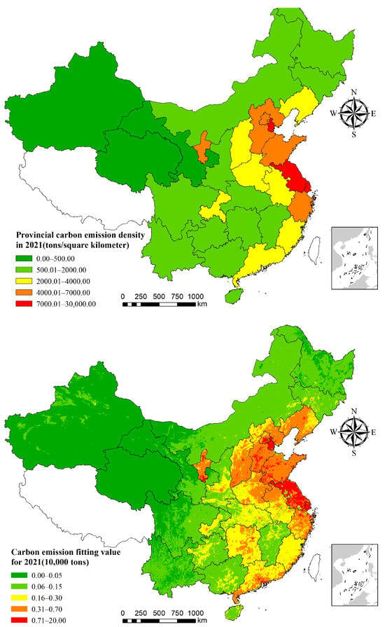
Figure 2.
Gridded carbon emission values before and after spatial fitting in 2021.
3.3. Study of the Dynamics of Spatial and Temporal Patterns
3.3.1. Provincial Scale
According to the calculation of the coefficient of variation (Figure 3a), the carbon emission levels of the 30 provinces in China were significantly different. In the global Moran’s I calculations, the Moran’s I for the years 2012 through 2021 passed the 0.05 significance test, and all the global Moran’s I values were greater than 0.2. From Figure 3, the overall distribution of carbon emissions can be inferred from the evolutionary pattern: China’s carbon emissions show positive geographical concentration characteristics, and the degree of aggregation slowly fluctuates to improve.
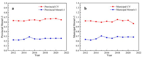
Figure 3.
Provincial (a) and municipal (b) scales of CV and Moran’s I.
The Moran scatter plot can reflect the carbon emission value of a unit relative to the surrounding units; from the first quadrant to the fourth quadrant they represent the “High–High”, “Low–High”, “Low–Low” and “High–Low” types, respectively. Taking the Moran scatterplot of provinces in 2012 and 2021 as an example (Figure 4), most of the provinces belonged to the “High–High” and “Low–Low” types, and there was a positive autocorrelation between provincial carbon emissions and provincial carbon emissions. Most of the provinces fell into the “High–High” and “Low–Low” categories, and there was a positive spatial autocorrelation of provincial carbon emissions. The number of provinces with the “Low–Low” type in the third quadrant was more than that of the “High–High” type in the first quadrant, which indicates that the number of low-value agglomerated units was higher, which is also an important part of the spatial positive autocorrelation of provincial carbon emissions. This is also an important part of the positive autocorrelation of provincial carbon emission space. The Moran scatterplot for the complete years is shown in Supplementary Materials Figure S2.
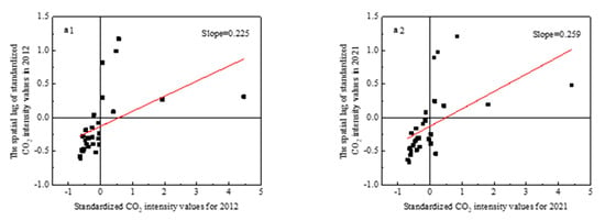
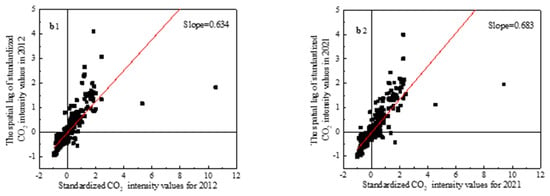
Figure 4.
Moran scatter plots at provincial (a) and municipal (b) scales.
According to the LISA agglomeration map in Figure 5 (years with the same LISA agglomeration map as the previous year are not shown due to space limitations), the spatial relationship distribution of carbon emissions at the provincial level in China is mainly a positively correlated agglomeration. The central inland, northeastern, and southeastern coastal regions of China were the most widely distributed non-significant regions. Except for the insignificant areas, the agglomeration types in each province were mainly of “High–High” and “Low–Low” types, and the number of “Low–Low” types was the largest. The “High–Low” type was only distributed during 2017–2021, while the “Low–High” type was never distributed. The “ Low–Low “ type was mainly found in the southwestern and northwestern provinces.
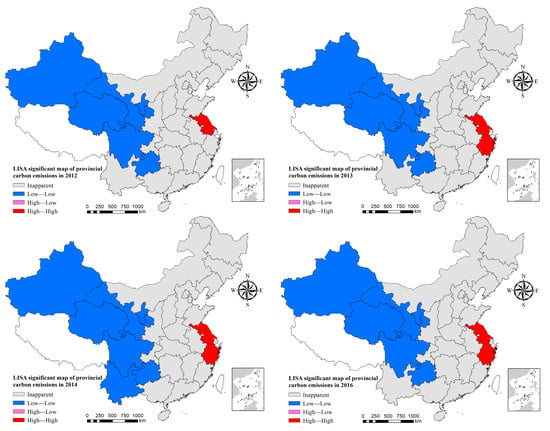
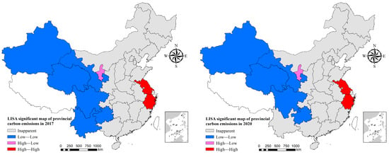
Figure 5.
LISA aggregation maps of carbon emission intensity at provincial scale.
The “High–High” type was mainly located in Jiangsu Province and Zhejiang Province, and after 2013, Zhejiang Province started to become a “High–High” type province due to its prominent manufacturing industry, with a wide range of textile, chemical, pharmaceutical, mechanical, and electronic industries. The textile, chemical, pharmaceutical, machinery, and electronics industries are widely developed, and these industries are among the main reasons for the increase in carbon emissions. Jiangsu Province is the second largest industrial province in China, leading the country in machinery, metallurgy, chemicals, and pharmaceuticals. Jiangsu and Zhejiang are not only the most populous provinces in China, they also have a strong industrial base. Due to the development of secondary industries and the rapid growth of energy extraction and production, these two provinces have been in a state of high energy consumption, which has led to a continuous increase in carbon emissions, and thus to the formation of a “High–High” type of agglomeration.
The “High–Low” type was mainly distributed in the Ningxia Hui Autonomous Region from 2017 to 2021. Ningxia is located in the western region and has the key responsibility of rational energy utilization. In recent years, Ningxia has prioritized a range of high-consumption chemical industries, such as coal refining, which has led to an increase in its average annual carbon emissions. However, the task of reducing carbon emissions is challenging because of the small size of its economy, its lack of growth momentum, and the fact that it relies heavily on transfer funds from the state. In addition, the Ningxia Hui Autonomous Region is also China’s major coal production and power generation base, making it difficult to reform its energy and industry layout. In the 13th Five-Year Plan, Ningxia successfully developed and operated a series of high-energy-consumption industries, and has also been responsible for relocating some of these industries, as well as transporting thermal power generation. The implementation of these key projects is the main reason why the energy consumption and carbon emissions per unit of GDP in the region have risen rather than fallen. On the other hand, Ningxia’s economic system is dominated by the secondary industry, especially the heavy manufacturing industry, while the share of the tertiary industry and high-tech industry is relatively small. With the construction of numerous coal processing plants and thermal power plants, its demand for renewable energy sources such as wind and solar energy has diminished, making it unable to carry out strong efforts to optimize its energy structure. These are the reasons why the Ningxia Hui Autonomous Region’s carbon emissions remain high and are significantly higher than those of neighboring provinces.
Further analysis of Figure 5 reveals that the type of Zhejiang has changed from a lack of clustering in 2012 to a “High–High” clustering distribution between 2013 and 2021. There was no “High–Low” category of provinces in the 2012–2016 period, but the Ningxia Hui Autonomous Region showed a “High–Low” agglomeration after 2017. The change in the “Low–Low” type is mainly reflected in two phases, one of which was in 2012–2016, when Ningxia no longer showed the “Low–Low“ type of agglomeration in the following years, and the other is that Yunnan showed the “Low–Low” type of agglomeration mainly in 2014–2019, while the remaining years were insignificant. The second is that the period in which Yunnan showed a “low–low” type of agglomeration was mainly concentrated in 2014–2019, with the remaining years being insignificant. Overall, the distribution patterns of carbon emissions in each year from 2012 to 2021 were relatively similar, with the only shifts occurring in Zhejiang, Ningxia, and Yunnan, and the spatial structure categories of provincial carbon emissions remained relatively stable.
3.3.2. Municipal Scale
The provincial spatial decomposition data were spatially counted in terms of prefecture-level cities to obtain the municipal carbon emission data from 2012 to 2021, and then the spatial and temporal patterns at the prefecture-level city scale were studied. According to the change in the coefficient of variation (Figure 3b), it can be found that the differentiated development of carbon emissions at the municipal level was heading in a different direction from the provincial level, and did not show a clear trend of growth or decrease. The CV was in a fluctuating state in the period and always stayed around 1.000. The global Moran’s I fluctuated from 0.634 in 2012 to 0.684 in 2021, which indicates that the spatial autocorrelation of carbon emissions of each city gradually increased.
Further analysis of Figure 3b shows that the CV and global Moran’s I did not follow the same trend, and sometimes their trends were clearly opposite. For example, during the period from 2012 to 2016, the CV decreased but the global Moran’s I increased. This indicates that during this period, although the differences in carbon emissions among Chinese cities were gradually decreasing, the trend of their spatial aggregation continued to intensify. The implementation of the “Development of the West” and “Rise of Central China” policies, coupled with changes in the industrial layout of the eastern region, have led to the relocation of some high-carbon emitting industries to the central and western regions. This has led to a massive expansion of local cities in the central and western regions, and has also led to a significant increase in carbon emissions. Nevertheless, according to the carbon emission distribution map, the east is still the focus of China’s social and economic development, and is a region with high carbon emissions. And during the period from 2017 to 2021, the CV and the global Moran’s I index showed a more synchronized pattern of fluctuation development, transitioning from the former pattern to a smoothing period, indicating that the regional distribution of China’s carbon emissions at the prefecture-level city scale has reached a more stable state.
Although it is not easy to find out the trend of the proportion of cities in the “high–high” and “low–low” categories over time by using only the data of the above-mentioned years, the dotted line graphs obtained from the data of the complete years show that the proportions of the cities in the “high–high” category and the “low–low” category have shown a more obvious fluctuating downward and fluctuating upward trend, respectively (Figure 6).
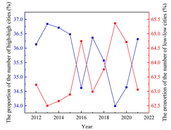
Figure 6.
Percentage of different types of cities.
Combined with the LISA agglomeration map, this phenomenon is not due to the transformation of some of the “High–High” cities into “Low–Low” cities, because the “High–High” and “Low–Low” cities are still located in the underdeveloped western region and the developed eastern region, respectively. “High–High” and “Low–Low” cities are still distributed in the underdeveloped western region and the developed eastern region, respectively. Therefore, the increase and decrease in the number of “High–High” and “Low-Low” cities is only due to the enhancement or weakening of localized agglomeration effects, and is not related to location. The decrease in the number of “High–High” cities in the east indicates that the regions with concentrated CO2 emissions have decreased, that is, the changes in industrial structure in some developed regions in the east have contributed to the reduction in carbon emissions. Similarly, the increased agglomeration effect in the western region is due to a shift in the agglomeration characteristics of some cities from insignificant to “Low–Low”. This can also explain the weakening of carbon emissions in the western region. Both of these changes are evidence of the good results of China’s vigorous implementation of energy-saving and emission-reduction policies.
From the Moran scatterplot of each city shown in Figure 4b, it can be seen that the slope in 2021 has a more prominent increase than that in 2019, which indicates that the spatial autocorrelation of carbon emissions in each prefecture-level city in China is gradually increasing [12]. The complete Moran scatterplot of each year can be found in Supplementary Materials Figure S3. Due to the space limitation, typical years with relatively prominent changes in the municipal LISA scatterplot were selected for analysis (Figure 7). It can be seen that the “High–High” cities in all the years are mainly concentrated in the Bohai Rim and the Yangtze River Delta; the “Low–Low” cities are mainly distributed in the central and western regions and Heilongjiang; the “Low–Low” cities are mainly distributed in the central and western regions and Heilongjiang; and the “Low–Low” cities are mainly distributed in the central and western regions and Heilongjiang. The “Low–Low” cities are mainly located in the central and western regions and Heilongjiang; the only “Low–High” city is Xuancheng, which has not formed a large agglomeration area. As a whole, the high carbon emission areas in North China and the Yangtze River Delta are the most prominent, and the western part of China is the main concentration area of “Low–Low” cities, and the spatial distribution range of such low carbon emissions is also decreasing.
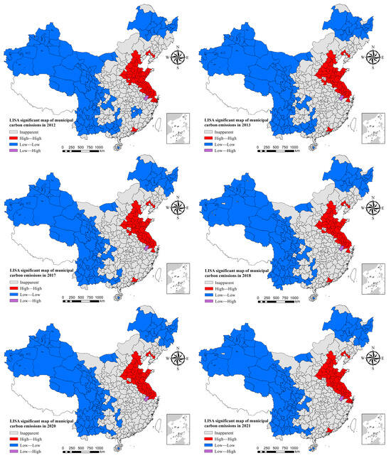
Figure 7.
LISA aggregation maps of carbon emission intensity at municipal scale.
4. Conclusions
This paper developed a method of multivariate variable extraction based on geographical categories and joint screening of multiple variables, and calculated the currently missing 1 km spatial distribution data of China’s carbon emissions from 2012 to 2021 by using SLM, which is capable of reflecting spatial linkages. This not only spatially filled in geographical areas not covered by previous studies, but also explored the spatial decomposition of carbon emissions on a large municipal scale that has not been conducted by previous researchers. The carbon emission regression parameters R2 and W_carbon both reflect the suitability of the land-class-based variable screening method and SLM. Especially at the municipal scale, the R2 reached approximately 0.99. This confirmed the excellent fitting ability of the method for carbon emissions. In other words, it can well establish the relationship between the dependent variable and the respective variables, and is a reliable method for spatial decomposition of carbon emissions, which greatly improves the accuracy of spatial decomposition of carbon emissions.
In the analysis of the spatial and temporal dynamics of carbon emissions, carbon emissions at the two scales showed different characteristics of changes in terms of spatial autocorrelation, which demonstrates the obvious influence of scale on regional disparities in carbon emissions. At smaller study scales, the discrete nature of China’s carbon emissions data is more pronounced and more likely to exhibit stronger spatial aggregation effects. In contrast, smaller spatial scales are more useful in showing the spatial dependence of territorial carbon emissions and their differentiated characteristics across space.
The spatial and temporal dynamics of carbon emissions could be projected for the period up to 2021. As can be seen from Figure 3a, provincial CVs and global Moran’s I showed positive geographic concentration characteristics, with a slowly fluctuating increase in the degree of aggregation, and did not show a significant downward trend. Combined with the distribution of LISA agglomeration types in Figure 5, it can be seen that future positive agglomerations will still be distributed in the eastern high-carbon emission zone and the western low-carbon emission zone, and the agglomeration effect is becoming more and more significant. Considering China’s current carbon emission reduction policy, the significance of this agglomeration effect may be brought about more by the “low–low” type in the western region in the future. As can be seen from Figure 3b, the differentiated development direction of carbon emissions at the municipal level is different from that at the provincial level, and does not show a clear trend of growth or decline, and it can be presumed that the future distribution of municipal carbon emissions will remain stable in this way.
5. Limitations and Perspectives
Although this paper adopted a variety of research methods and obtained a series of characteristics of carbon emission distribution in China. However, there are still areas that need to be optimized and improved, and many difficult issues still need to be studied in depth.
Due to the constraints of data collection, this paper was unable to comprehensively understand the carbon emission statistics of Tibet Autonomous Region, Hong Kong, Macao, Taiwan, and some cities at the municipal scale. In the future exploration process, collecting data related to carbon emissions from more regions and distributing carbon emission data to each region at a fine scale is an optimized direction for the spatial decomposition study of China’s carbon emissions in the future.
Although the SLM chosen in this paper was based on previous research and determined after weighing the effects, the time and spatial scopes of the previous research were not exactly the same as this paper. After the practice of this paper, the regression effect of SLM was confirmed to be excellent. However, how to find a more appropriate model according to the characteristics of China’s socio-economic spatial differences will become the main theoretical path to explore the spatial decomposition of China’s carbon emissions in the future.
Supplementary Materials
The following supporting information can be downloaded at https://www.mdpi.com/article/10.3390/atmos15050538/s1, Figure S1: Fitted value of our 1-km GDP in 2012 and 2021; Figure S2: Moran scatterplot of provincial scale carbon emissions; Figure S3: Moran scatterplot of carbon emissions at municipal scale; Table S1: Table of rotated component matrices; Table S2: Subsumption of carbon emission independent variables on land classification; Table S3: Correlation analysis of initially screened independent variables; Table S4: Parameter table of provincial SLM regression coefficients for 2021.
Author Contributions
Conceptualization, M.W., X.D. and H.Z.; Data curation, M.W.; formal analysis, M.W.; funding acquisition, M.W.; investigation, M.W.; methodology, M.W., X.D. and H.Z.; project administration, M.W. and X.D.; resources, M.W., X.D. and H.Z.; software, M.W.; supervision, X.D.; validation, M.W.; visualization, M.W.; writing—original draft, M.W.; Writing—review and editing, X.D. All authors have read and agreed to the published version of the manuscript.
Funding
This research received no external funding.
Institutional Review Board Statement
Not applicable.
Informed Consent Statement
Not applicable.
Data Availability Statement
Publicly available datasets were analyzed in this study. This data can be found here: https://lpdaac.usgs.gov/products/; https://landscan.ornl.gov/; https://payneinstitute.mines.edu/eog/nighttime-lights/; https://data.cnki.net/home; https://www.ceads.net/.
Conflicts of Interest
The authors declare no conflict of interest.
Glossary
| Term | Definition |
| SLM | An important model in spatial econometrics to characterize spatial correlation and spatial dependence. |
| downscaled spatial decomposition | Allocating carbon emissions to smaller scale units allows carbon emissions data to be distributed at finer scales. |
| carbon emission | The value of cumulative carbon dioxide emitted into the air, which in this paper refers specifically to carbon emissions caused by human activities. |
| fitting or regression | The process of model fit between dependent and independent variables. |
| image or raster | A basic unit of data storage in GIS, the size of which is expressed in terms of the length of a side. |
References
- Shi, K.; Shen, J.; Wu, Y.; Liu, S.; Li, L. Carbon dioxide (CO2) emissions from the service industry, traffic, and secondary industry as revealed by the remotely sensed nighttime light data. Int. J. Digit. Earth 2021, 14, 1514–1527. [Google Scholar] [CrossRef]
- Wei, W.; Zhang, X.; Cao, X.; Zhou, L.; Xie, B.; Zhou, J.; Li, C. Spatiotemporal dynamics of energy-related CO2 emissions in China based on nighttime imagery and land use data. Ecol. Indic. 2021, 131, 108132. [Google Scholar] [CrossRef]
- Zhou, A.; Xin, L.; Li, J. Assessing the impact of the carbon market on the improvement of China’s energy and carbon emis-sion performance. Energy 2022, 258, 124789. [Google Scholar] [CrossRef]
- Chen, H.; Zhang, X.; Wu, R.; Cai, T. Revisiting the environmental Kuznets curve for city-level CO2 emissions: Based on corrected NPP-VIIRS nighttime light data in China. J. Clean. Prod. 2020, 268, 121575. [Google Scholar] [CrossRef]
- Wu, X.; Huang, Y.; Gao, J. Impact of industrial agglomeration on new-type urbanization: Evidence from Pearl River Delta urban agglomeration of China. Int. Rev. Econ. Financ. 2022, 77, 312–325. [Google Scholar] [CrossRef]
- Chen, W.; Wang, G.; Xu, N.; Ji, M.; Zeng, J. Promoting or inhibiting? New-type urbanization and urban carbon emissions efficiency in China. Cities 2023, 140, 104429. [Google Scholar] [CrossRef]
- Chevallier, F.; Zheng, B.; Broquet, G.; Ciais, P.; Liu, Z.; Davis, S.J.; Deng, Z.; Wang, Y.; Breon, F.-M.; O’Dell, C.W. Local Anomalies in the Column-Averaged Dry Air Mole Fractions of Carbon Dioxide Across the Globe During the First Months of the Coronavirus Recession. Geophys. Res. Lett. 2020, 47, e2020GL090244. [Google Scholar] [CrossRef] [PubMed]
- Liu, X.; Ou, J.; Wang, S.; Li, X.; Yan, Y.; Jiao, L.; Liu, Y. Estimating spatiotemporal variations of city-level energy-related CO2 emissions: An improved disaggregating model based on vegetation adjusted nighttime light data. J. Clean. Prod. 2018, 177, 101–114. [Google Scholar] [CrossRef]
- Wang, L.; Zhang, Y.; Zhao, Q.; Ren, C.; Fu, Y.; Wang, T. Horizontal CO2 Compensation in the Yangtze River Delta Based on CO2 Footprints and CO2 Emissions Efficiency. Int. J. Environ. Res. Public Health 2023, 20, 1369. [Google Scholar] [CrossRef]
- Ma, Q.; He, C.; Wu, J. Behind the rapid expansion of urban impervious surfaces in China: Major influencing factors re-vealed by a hierarchical multiscale analysis. Land Use Policy 2016, 59, 434–445. [Google Scholar] [CrossRef]
- Wang, H.; Liu, G.; Shi, K. What Are the Driving Forces of Urban CO2 Emissions in China? A Refined Scale Analysis between National and Urban Agglomeration Levels. Int. J. Environ. Res. Public Health 2019, 16, 3692. [Google Scholar] [CrossRef] [PubMed]
- Shi, K. A Study on the Dynamics of Spatial and Temporal Patterns of Carbon Emissions and Influencing Factors in China from a Multi-Scale Perspective. Ph.D. Thesis, Shanghai East China Normal University, Shanghai, China, 2017. [Google Scholar]
- Chen, J.; Gao, M.; Cheng, S.; Liu, X.; Hou, W.; Song, M.; Li, D.; Fan, W. China’s city-level carbon emissions during 1992–2017 based on the inter-calibration of nighttime light data. Sci. Rep. 2021, 11, 3323. [Google Scholar] [CrossRef] [PubMed]
- Meng, X.; Han, J.; Huang, C. An Improved Vegetation Adjusted Nighttime Light Urban Index and Its Application in Quan-tifying Spatiotemporal Dynamics of Carbon Emissions in China. Remote Sens. 2017, 9, 829. [Google Scholar] [CrossRef]
- Zhang, J.; Feng, Z.; Jiang, L. Advances in Land Use/Land Cover Classification Systems. Resour. Sci. 2011, 33, 1195–1203. [Google Scholar]
- Elvidge, C.D.; Baugh, K.; Zhizhin, M.; Hsu, F.C.; Ghosh, T. VIIRS night-time lights. Int. J. Remote Sens. 2017, 38, 5860–5879. [Google Scholar] [CrossRef]
- Elvidge, C.D.; Zhizhin, M.; Ghosh, T.; Hsu, F.-C.; Taneja, J. Annual Time Series of Global VIIRS Nighttime Lights Derived from Monthly Averages: 2012 to 2019. Remote Sens. 2021, 13, 922. [Google Scholar] [CrossRef]
- Guan, Y.; Shan, Y.; Huang, Q.; Chen, H.; Wang, D.; Hubacek, K. Assessment to China’s Recent Emission Pattern Shifts. Earths Future 2021, 9, e2021EF002241. [Google Scholar] [CrossRef]
- Shan, Y.; Huang, Q.; Guan, D.; Hubacek, K. China CO2 emission accounts 2016–2017. Sci. Data 2020, 7, 54. [Google Scholar] [CrossRef] [PubMed]
- Shan, Y.; Guan, D.; Zheng, H.; Ou, J.; Li, Y.; Meng, J.; Mi, Z.; Liu, Z.; Zhang, Q. Data Descriptor: China CO2 emission accounts 1997–2015. Sci. Data 2018, 5, 170201. [Google Scholar] [CrossRef]
- Shan, Y.; Liu, J.; Liu, Z.; Xu, X.; Shao, S.; Wang, P.; Guan, D. New provincial CO2 emission inventories in China based on apparent energy consumption data and updated emission factors. Appl. Energy 2016, 184, 742–750. [Google Scholar] [CrossRef]
- Shan, Y.; Guan, Y.; Hang, Y.; Zheng, H.; Li, Y.; Guan, D.; Li, J.; Zhou, Y.; Li, L.; Hubacek, K. City-level emission peak and drivers in China. Sci. Bull. 2022, 67, 1910–1920. [Google Scholar] [CrossRef]
- Shan, Y.; Guan, D.; Hubacek, K.; Zheng, B.; Davis, S.J.; Jia, L.; Liu, J.; Liu, Z.; Fromer, N.; Mi, Z.; et al. City-level climate change mitigation in China. Sci. Adv. 2018, 4, eaaq0390. [Google Scholar] [CrossRef] [PubMed]
- Shan, Y.; Guan, D.; Liu, J.; Mi, Z.; Liu, Z.; Liu, J.; Schroeder, H.; Cai, B.; Chen, Y.; Shao, S.; et al. Methodology and appli-cations of city level CO2 emission accounts in China. J. Clean. Prod. 2017, 161, 1215–1225. [Google Scholar] [CrossRef]
- Shan, Y.; Liu, J.; Liu, Z.; Shao, S.; Guan, D. An emissions-socioeconomic inventory of Chinese cities. Sci. Data 2019, 6, 190027. [Google Scholar] [CrossRef] [PubMed]
- Ma, T.; Zhou, C.; Pei, T.; Haynie, S.; Fan, J. Responses of Suomi- NPP VIIRS- derived nighttime lights to socioeconomic activity in China’s cities. Remote Sens. Lett. 2014, 5, 165–174. [Google Scholar] [CrossRef]
- Liang, H.; Guo, Z.; Wu, J.; Chen, Z. GDP spatialization in Ningbo City based on NPP/VIIRS night-time light and auxiliary data using random forest regression. Adv. Space Res. 2020, 65, 481–493. [Google Scholar] [CrossRef]
- Wang, X.; Sutton, P.C.; Qi, B. Global Mapping of GDP at 1 km2 Using VIIRS Nighttime Satellite Imagery. Isprs Int. J. Geo-Inf. 2019, 8, 580. [Google Scholar] [CrossRef]
- Wang, Y.; Teng, F.; Wang, M.; Li, S.; Lin, Y.; Cai, H. Monitoring Spatiotemporal Distribution of the GDP of Major Cities in China during the COVID-19 Pandemic. Int. J. Environ. Res. Public Health 2022, 19, 8048. [Google Scholar] [CrossRef] [PubMed]
- Huang, Y.; Chen, W.; Zhang, Z. Spatial Gridding of GDP in Fujian Province Based on Multi-source Data. J. Hubei Coll. Natl. Nat. Sci. Ed. 2018, 36, 103–109. [Google Scholar]
- Liu, Y.; Yan, Q. Simulation of Spatial Distribution of Carbon Emission Gridding in China Based on SLM Model. Geogr. Geogr. Inf. Sci. 2015, 31, 76–80. [Google Scholar]
- Pan, J.; Zhao, X. Simulation of spatial differences in carbon emissions in China based on spatial regression modeling. J. Environ. Sci. 2018, 38, 2894–2901. [Google Scholar]
- Christopher, N.H.D.; Jan-Peter, M.; Christopher, D.E. Night-time Imagery as a Tool for Global Mapping of Socioeconom-ic Parameters and Greenhouse Gas Emissions. AMBIO A J. Hum. Environ. 2000, 29, 157–162. [Google Scholar]
- Zhang, G.; Guo, X.; Li, D.; Jiang, B. Evaluating the Potential of LJ1-01 Nighttime Light Data for Modeling Socio-Economic Parameters. Sensors 2019, 19, 1465. [Google Scholar] [CrossRef] [PubMed]
- Liu, H.; Luo, N.; Hu, C. Detection of County Economic Development Using LJ1-01 Nighttime Light Imagery: A Compari-son with NPP-VIIRS Data. Sensors 2020, 20, 6633. [Google Scholar] [CrossRef] [PubMed]
- Wang, L.; Zhang, N.; Deng, H.; Wang, P.; Yang, F.; Qu, J.J.; Zhou, X. Monitoring urban carbon emissions from energy con-sumption over China with DMSP/OLS nighttime light observations. Theor. Appl. Climatol. 2022, 149, 983–992. [Google Scholar] [CrossRef]
- Guo, X.; Yan, Q.; Tan, X.; Liu, S. Simulation of spatial distribution of carbon emissions in Jiangsu Province based on DMSP/OLS and NDVI. World Geogr. Res. 2016, 25, 102–110. [Google Scholar]
- Lv, M.; Zhong, Y. Advances in the application of NDVI in ecological research. Rural Econ. Sci. Technol. 2011, 22, 11–14. [Google Scholar]
- Poumanyvong, P.; Kaneko, S. Does urbanization lead to less energy use and lower CO2 emissions? A cross-country analysis. Ecol. Econ. 2010, 70, 434–444. [Google Scholar] [CrossRef]
- Zhang, T.; Song, Y.; Yang, J. Relationships between urbanization and CO2 emissions in China: An empirical analysis of population migration. PLoS ONE 2021, 16, e0256335. [Google Scholar] [CrossRef]
- Li, X.; Wang, X.; Zhang, S. Impacts of Urban Spatial Development Patterns on Carbon Emissions: Evidence from Chinese Cities. Land 2022, 11, 2031. [Google Scholar] [CrossRef]
- Desmet, K.; Gomes, J.F.; Ortuño-Ortín, I. The geography of linguistic diversity and the provision of public goods. J. Dev. Econ. 2020, 143, 102384. [Google Scholar] [CrossRef]
- Hu, Y.; Qi, C. A Study of Economic Development Differences among Economies within the China-ASEAN FTA. Econ. Geogr. 2013, 33, e0282167. [Google Scholar]
- Ma, X.; Li, Q.; Shen, Y. Morphological differentiation and geographic types of rural settlements in Jiangsu Province. J. Geogr. 2012, 67, 516–525. [Google Scholar]
- Wang, S.; Zhang, S.; Cheng, L. Investigating the Synergy between CO2 and PM2.5 Emissions Re-duction: A Case Study of China’s 329 Cities. Atmosphere 2023, 14, 1338. [Google Scholar] [CrossRef]
- Le Gallo, J.; Ertur, C. Exploratory spatial data analysis of the distribution of regional per capita GDP in Europe, 1980–1995. Pap. Reg. Sci. 2003, 82, 175–201. [Google Scholar] [CrossRef]
- Bai, J.; Li, S.; Kang, Q.; Wang, N.; Guo, K.; Wang, J.; Cheng, J. Spatial Spillover Effects of Renewable Energy on Carbon Emissions in Less-developed Areas of China. Environ. Sci. Pollut. Res. 2022, 29, 19019–19032. [Google Scholar] [CrossRef]
Disclaimer/Publisher’s Note: The statements, opinions and data contained in all publications are solely those of the individual author(s) and contributor(s) and not of MDPI and/or the editor(s). MDPI and/or the editor(s) disclaim responsibility for any injury to people or property resulting from any ideas, methods, instructions or products referred to in the content. |
© 2024 by the authors. Licensee MDPI, Basel, Switzerland. This article is an open access article distributed under the terms and conditions of the Creative Commons Attribution (CC BY) license (https://creativecommons.org/licenses/by/4.0/).