Data-Driven Prediction of Severe Convection at Deutscher Wetterdienst (DWD): A Brief Overview of Recent Developments

Abstract

Thunderstorms endanger life and infrastructure. The accurate and precise prediction of thunderstorms is therefore helpful to enable protection measures and to reduce the risks. This manuscript presents the latest developments to improve thunderstorm forecasting in the first few hours. This includes the description and discussion of a new Julia-based method (JuliaTSnow) for the temporal extrapolation of thunderstorms and the blending of this method with the numerical weather prediction model (NWP) ICON. The combination of ICON and JuliaTSnow attempts to overcome the limitations associated with the pure extrapolation of observations with atmospheric motion vectors (AMVs) and thus increase the prediction horizon. For the blending, the operational ICON-D2 is used, but also the experimental ICON-RUC, which is implemented with a faster data assimilation update cycle. The blended products are evaluated against lightning data. The critical success index (CSI) for the blended RUC product is higher for all forecast time steps. This is mainly due to the higher resolution of the AMVs (prediction hours 0–2) and the rapid update cycle of ICON-RUC (prediction hours 2–6). The results demonstrate the potential of the rapid update cycle to improve the short-term forecasts of thunderstorms. Moreover, the transition between AMV-driven nowcasting to NWP is much smoother in the blended RUC product, which points to the advantages of fast data assimilation for seamless predictions. The CSI is well above the critical value of 0.5 for the 0–2 h forecasts. Values below 0.5 mean that the number of hits (correct informations) is lower than the number of failures, which results from the missed cells plus false alarms. The product is then no longer useful in forecasting thunderstorms with a spatial accuracy of 0.3 degrees. Unfortunately, with RUC, the CSI also drops below 0.5 when the last forecast is more than 3 h away from the last data assimilation, indicating the lack of model physics to accurately predict thunderstorms. This lack is simply a result of chaos theory. Within this context, the role of NWP in comparison with artificial intelligence (AI) is discussed, and it is concluded that AI could replace physical short-term forecasts in the near future.

1. Introduction

Thunderstorms, which are produced by cumulonimbus clouds (Cb) through electrical discharge, occur frequently during the summertime in many regions of the world. They are often accompanied by wind gusts, heavy precipitation, hail and turbulence. These weather events can lead to serious local floods, harvest failures and damage to infrastructure. Further, around the world, humans are often killed by lightning strikes. In aircraft, passengers are well protected against lightning as a result of the phenomenon known as the Faraday cage. However, thunderstorms are usually associated with turbulence, and these are one of the most common reasons for injuries in aviation. These examples illustrate that it is important to determine the occurrence and expected severity of thunderstorms well in advance in order to protect infrastructure and human life.

Thunderstorm detection and monitoring is offered by operators of lightning detection networks; see [1,2,3,4,5,6]. However, these services are commercial and do not use satellite information for the nowcasting of thunderstorms. Nowcasting is referenced here and throughout the manuscript as the temporal extrapolation of observations for 0–2 h. In Europe, one of the first entities to provide software for satellite-based thunderstorm nowcasting was the Nowcasting Application Facility (NWC-SAF) [7], but, for application at DWD, this software was not suitable, as discussed in detail in [8]. As a result, the NowCastSat-Aviation (NCS-A) method was developed and implemented at Deutscher Wetterdienst as an operational 24/7 product in DWD’s High-Performance Computer (HPC) with ecflow [9].

NCS-A provides the near-real-time detection and prediction of convective cells across the global domain using geostationary satellites in combination with lightning data and information from numerical weather prediction. The satellites used for NCS-A are METEOSAT, the European METEOrological SATellite [10], GOES, the US Geostationary Operational Environmental Satellite [11] and HIMAWARI [12], which means “sunflower” in English. In 2023, the weather satellite GK2A [13], operated by the Korean Meteorological Administration (KMA), was added. Lightning data from VAISALA [2,3,4,5,6] are used to highlight heavy convection and to reduce the false alarms and missed cells during the detection step, which would be incurred if only satellites were used. The GLD360 data cover the entire globe and are based on Broadband VLF Radio Reception [14].

The NCS-A product is provided in three different severity levels. The light and moderate severity levels are defined mainly by the brightness temperatures (BTs) derived from the SEVIRI water vapor (WV) channels. Light convection is defined for satellite pixels with a brightness temperature difference in the water vapor channels (BT_6.2–BT_7.3) larger than −1 and a convective KO index of less than 2. The latter condition is used to reduce false alarms as not all cold clouds are thunderstorm clouds; see [15] for details. The KO index is a measure of the instability of the atmosphere (see Appendix A) and is derived from the numerical weather prediction model ICON [16]. For moderate convection, the clouds need to be colder, i.e., greater than 0.7 for the difference in the water channels ($WV063-WV073>0.7$) and greater than 2 for the BT difference in the water vapor channel and the window channel ($WV062-IR10.8>2$). The latter condition can be used to identify overshooting tops, which are an indicator of strong updrafts associated with severe turbulence and hail [17,18,19,20]. The occurrence of lightning data is a prerequisite for the identification of the severe level. As a consequence, the severe level is usually surrounded by the light or moderate levels. All lightning measurements occurring 15 min before the end of the latest satellite scan are taken into account. For nowcasting, two subsequent satellite images of the water vapor channel (ca. 6.2 $\mathsf{\mu }$m) from different geostationary satellites are used. These images are fed into the optical flow method TV-L1 [21], which is provided as part of OpenCV [22,23]. The latest image is then extrapolated in time based on the estimated atmospheric flow. Forecasts are calculated every 15 min and cover lead times up to 2 h after the latest satellite scan, with a temporal resolution of 15 min and a spatial resolution of 0.1 degrees (ca. 10 km). The nowcasting, including the processing of the satellite, lightning and NWP data, is performed with a software package developed at DWD, referred to as Geotools. The Geotools package is written in Python (version 3.6), using Pytroll [24], for the reading of satellite data and georeferencing. More detailed information about NCS-A can be found in [8]

Another global Cb nowcasting product is based on the Convective Diagnosis Oceanic (CDO) algorithm. It is used to detect the areas of thunderstorms that are most hazardous for aviation through a combination of geostationary satellite-based data and ground-based lightning data. A simple fuzzy logic approach is used to combine the information from different input fields. The CDO input fields are the cloud top height, the Global Convective Diagnosis [25], the Overshooting Tops Detection algorithm [17] and the EarthNetworks global, ground-based lightning detection network [26]. On a regional scale, radar data can be used for nowcasting as well, e.g., NowCastMIX-Aviation (NCM-A) [27].

Atmospheric motion vectors (AMVs) are typically used to predict the movement of cloud objects in satellite-based physical nowcasting methods, whereby at least two subsequent satellite images are needed for their calculation. Different methods can be applied for the calculation of the AMVs, as discussed in more detail in [28]. In modern applications, AMVs are typically gained from optical flow methods. DWD has good experience with modern computer vision techniques, e.g., [21,29,30]. They can be easily adapted to the different application fields as they provide a dense vector field based on a multi-scale approach. The parameters can be optimized for the respective application. Optical flow is used at DWD for the nowcasting of thunderstorms [8], turbulence [31], solar surface irradiance [28] and precipitation/radar [27,32].

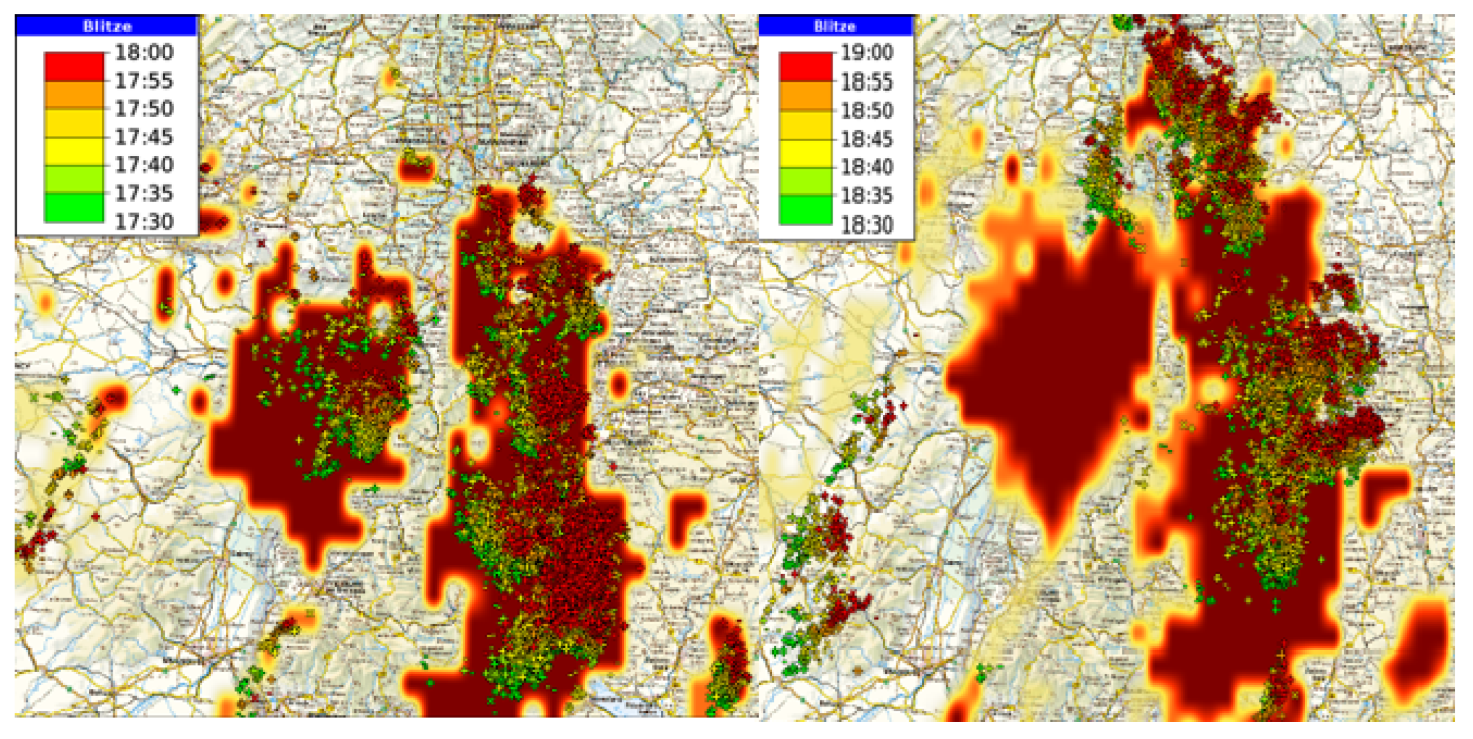
However, temporal extrapolation with AMVs only considers the movement of cells. Life cycle features, e.g., the dissipation or development cells, are not captured. However, a typical feature of convection is that the cells do not stay constant, but grow or dissipate. Hence, a central assumption of the optical flow is violated, namely that the intensity of the objects does not change. Thus, atmospheric motion vectors are limited not only by the fact that they only describe the movement, but also by an increase in errors in the estimated advection in the presence of strong convection. Thus, the number of false alarms and missed cells increases considerably as the forecast time increases. The critical value of around 0.5 is usually reached for CSI after 90 min of prediction time and then drops off rapidly, regardless of the chosen optical flow method; see, e.g., [8,33]. This limitation is an inherent feature and applies to all atmospheric motion vector methods, as illustrated in Figure 1. This has motivated further developments to improve the accuracy and extend the forecast length. This includes adjustments of the nowcasting and its combination with numerical weather prediction.

Within this context, this manuscript provides an overview of recent developments concerning thunderstorm prediction at DWD. In the first part (Section 2.1), purely data-driven thunderstorm nowcasting will be discussed, with a subsection for cloud top height information, which is a typical companion for thunderstorm nowcasting. Afterwards, in Section 2.2, the analysis of the NWP ensembles is presented, which is used to prolong the data-driven nowcasting to 0–6 h. In order to combine the nowcasting and the NWP-based forecasts, a blending method is needed, which is described in Section 2.3. The evaluation of the resulting 0–6 h forecasts is discussed in Section 3. The paper closes with a discussion of the evaluation results and a conclusion, whereby also the strengths and weaknesses of the physical approach are discussed in relation to data-driven AI-based nowcasting approaches, e.g., [33]. The blended TS products are presented and discussed in this manuscript for the first time, as well as the open data products, CTH and the extensions of NCS-A.

2. Materials and Methods: Six-Hour Forecast of Severe Convection

The prediction of thunderstorms for the time range of 0–6 h is achieved by a combination of the lightning potential index (LPI) of the numerical weather prediction model ICON and the observational-based nowcasting of thunderstorms. In the following, the methods to generate the 0–6 h forecasts are described in more detail. First, the nowcasting method is described, followed by a description of the analysis of the ensembles $LP{I}_{MAX}$ and the method for blending.

2.1. Nowcasting Methods

2.1.1. JuliaTSnow

In order to ensure a good basis for the transition of the nowcasting to the analysis of the lightning potential index (LPI), the NCS-A approach has been modified. This was also done to test further potential improvements in the method and the Julia programming language [34]), which promises higher computing performance compared to Python. This in turn is of great importance for big data applications. The Python-based NCS-A method needs almost 15 min in 10 km resolution (geostationary ring) and 8–12 after optimization, which represents a breakthrough in the capabilities provided by MTG/FCI [35]. Below, the main differences in the JuliaTSnow nowcasting method compared to NCS-A are discussed.

The nowcasting method JuliaTSnow was developed explicitly for thunderstorms. Thus, deep convection without the occurrence of lightning strikes is not covered by the method. As mentioned, the LPI is used as a proxy for thunderstorms on the model side. Thus, the basis for the detection of thunderstorms in the nowcasting part is based on lightning as well. This is a significant difference compared to NCS-A, where light and moderate convection can be classified without the occurrence of flashes.

Further, the optical flow method TV-L1 is replaced by Farnebäck, which works reasonably well for thunderstorms. Farnebäck is faster and more robust concerning static cells, but is unfortunately also more sensitive to changes in intensity than TV-L1. In essence, two subsequent images of the brightness temperature differences in the water vapor channels (BTDWV: BT_6.2–BT_7.3) are used [15] for the calculation of the optical flow. However, the optical flow method requires images within the range of 0–1; hence, the BT differences are normalized with a maximum value of 10 and a minimum of −4. The range is defined in order to focus on medium to optically thick clouds. This improves the quality of the AMVs but increases also the computing speed. Please note that these temperatures are by no means comparable to the BT temperature in the infrared (IR) window channels, e.g., the difference results in positive temperatures even for medium to cold clouds. Negative temperatures indicate, in this case, that the clouds are close to the tropopause.

Finally, the severity is defined in another manner. In both methods, the severity depends on how cold the clouds are, as a consequence of the relation between the severity and brightness temperature, e.g., [36]. NCS-A comes with three severity levels, but JuliaTSnow provides continuous values from 0 to 1 for the severity of thunderstorms. The severity is defined as follows.

$$SEV[i,j]={\left(sin(1.68\ast dB{T}_{norm}[i,j])\right)}^8$$

(1)

$SEV$ is the severity, and $\ast dB{T}_{norm}$ is the normalized brightness temperature difference for the pixels at location $i,j$.

The JuliaTSNow approach provides TS nowcasting for Europe and Africa and needs only 2 min for the completion of the nowcast. The occurrence of at least one lightning event within a 10 min interval and a search radius of 1 pixel are the preconditions for the detection of a thunderstorm cell. JuliaTSnow is operated in two modes. The first is as a standalone tool covering Europe, Africa and the surrounding oceans. In this mode, the global GLD360 lightning data [2,3,4,5,6] are used. The respective TS nowcasting (0–90 min) is available on the DWD data server as a standalone product in 15 min and a 0.05 degree resolution in cf conform netcdf format [37].

In the other mode, only Central Europe is covered, and this mode is operated for data fusion with ICON-D2 and ICON-RUC; see Section 2.3. This region is well covered by the regional LINET data [1,38], which offers a higher density of lightning data. This is an advantage for blending with ICON. As a consequence of the combination with ICON, the forecast horizon is extended to 0–6 h in this mode. The respective data are not available as open data.

Information about the cloud top height of thunderstorms is an important prerequisite for many applications, including thunderstorm nowcasting; thus, a smart CTH approach is briefly described below.

2.1.2. Prediction by Visual Inspection—Cloud Top Height

The cloud top height is well suited for the visual analysis and nowcasting of thunderstorms and weather impacting clouds and offers more generally the option for the early detection of developing convection. It is one of the most used satellite-based products for the visual inspection of the development of thunderstorms at DWD.

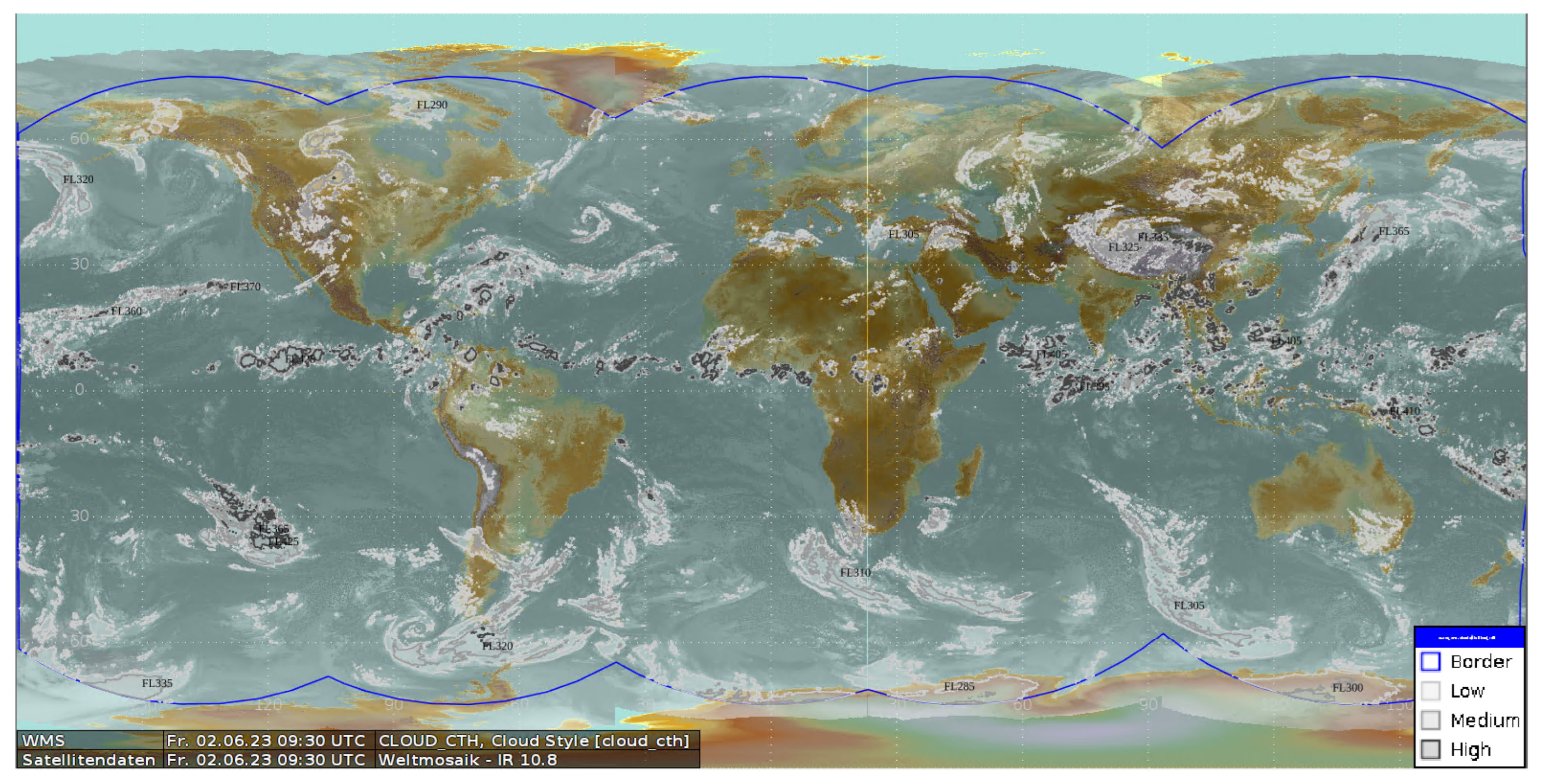
Further, in many applications, particularly dealing with aviation, the severity information of the thunderstorm or severe convection is accompanied by the cloud top height information. Moreover, NCS-A provides cloud top height information for deep convection, whereby an NWP filter is applied for light convection. However, aviation operators require height information for all optically thick clouds without NWP filtering in order to obtain a global scan of the weather active zones in the cockpit as well. For this reason, a cloud map option has been added to NCS-A with a discrete distinction between low, medium and high clouds; see Figure 2.

Before a CTH can be calculated, a cloud mask is needed. As the focus of the CTH product for aviation lies in optically thick clouds, the brightness temperature difference (BTD) of the water vapor channels with a BTD threshold of about −8 to −10 can be used [17,39]. Optically thick clouds are opaque in the IR. Hence, in good approximation, the observed BT equals the temperature of the cloud top. For opaque clouds, the cloud top height can be defined as follows:

$$CTH=-(B{T}_{IRW}-T_{tropo})/LR+H_{tropo}$$

(2)

Here, $B{T}_{IRW}$ is the brightness temperature of the IR window channel (∼10.8 $\mathsf{\mu }$m), and $T_{tropo}$ and $H_{tropo}$ are the temperature and height of the tropopause from the numerical weather prediction model ICON [16] or similar climatologies. LR is the lapse rate and is set to 8.0 [K/km] for NCS-A [8,15,31].

For the aviation-specific CTH product, three height levels are defined from the requirements of NCS-A users, which are FL250 (7.6 km), FL325 (9.9 km) and FL400 (12.2 km). The following CTHs and BTD thresholds are used for the definition of the three levels, see

Table 1. Overview of the definition of the three cloud height regimes and their possible relation to the life cycle of deep convection. BTD is the difference in the water vapor channels.

Vertical Thickness	Threshold	In Case of Convection
medium	$BT{D}_{WV}$ > −8 and $CTH$ > FLT250	early stage
high	$BT{D}_{WV}$ > −4 and $CTH$ > FLT325	developing
very high	$BT{D}_{WV}$ > 1 and $CTH$ > FLT400	deep convection

. Cloud heights greater than FL400 should indicate areas where flying over the clouds is not advisable due to a possible stall (coffin corner).

While discrete height information is sufficient for the NCS-A product, continuous CTH products have established themselves in general weather forecasting. Further, for the combined use of CTH with radar reflectivities, a parallax-corrected CTH product is of great benefit. This motivated the development of a standalone CTH product for Europe. As this product includes all clouds and not only optically thick clouds, a different cloud mask is needed. The respective cloud mask results from the adaptation of the CALSAT method [40] to the infrared window channel (10.6). As a consequence, the cloud top height (CTH) is then calculated for cloudy pixels with Equation (2). However, in this case, the $H_{tropo}$ and $T_{tropo}$ information comes from standard climatological profiles for ease of use and to avoid model contamination. Thus, in contrast to other methods, no information from numerical weather prediction (NWP) is needed. Further, in contrast to NCS-A, the lapse rate is assumed to be 6.5 K/km in accordance with ICAO_93. This difference is motivated by the fact that NCS-A is only applied to deep convection, whereas the CTH open data product covers all cloud types.

For semitransparent clouds, a correction of the CTH is needed, which can be done with a method referred to as the water vapor H2O intercept method [31]. The CTH open data product [41] is provided as a cf-conform netcdf file in a regular grid, with a spatial resolution of 0.05 × 0.05 degrees and a temporal resolution of 15 min (10 min with MTG). The height is given in m. An example of the product is provided in Figure 3. For combined use with radar data, the CTH product is parallax-corrected using a function from the Julia satellite library. This library is available on request. The basic geometric equation in this function is from Eumetsat.

2.2. Thunderstorm Forecast with LPI

Numerical weather models (NWP) contain physics, which allows them to simulate the life cycles of cells and thus the dissemination and development of cells. Hence, there might be potential to improve and extend reliable thunderstorm prediction by blending data-driven nowcasting with numerical weather prediction. Of course, due to the complex and partly chaotic thermodynamics, the accurate simulation of the processes is quite difficult. A central aspect to improve the forecast quality is data assimilation, as this forces the system to model the real atmospheric conditions. Within this context, one aim is the use of as many observational data as possible in order to define the initial state of the atmosphere, ensuring that the data assimilation is as successful as possible. On average, the higher the uncertainty of the initial state, the higher the uncertainty of the simulated weather. Moreover, great progress has been made to improve the definition of the initial state, e.g., by the use of data from new satellite generations, but there is still the significant underdetermination of the initial state. Further, the model physics induces uncertainties in the forecasts. To account for these uncertainties, weather services have implemented the option for ensemble forecasts, which are also used in this study.

Thunderstorms are among the most chaotic weather phenomena. Based on the theory of Lorenz [42], it is expected that a faster update cycle in data assimilation leads to better accuracy, particularly for short-term forecasts. This will be further investigated and discussed in Section 4 after the presentation of the results.

In this study, the regional NWP model ICON is used for the combined product. The ICOsahedral Nonhydrostatic D2 [16,43] is a nonhydrostatic model that enables improved forecasts of hazardous weather conditions with high-level moisture convection (super- and multi-cell thunderstorms, squall lines, mesoscale convective complexes) due to its improved physics in combination with its fine mesh size. The domain of ICON-D2 covers Germany and the bordering countries with a spatial resolution of 2.2 km. For ICON-D2, data assimilation is applied every 3 h, and a complete model run needs approximately 2 h.

ICON-D2 is the current operational model at DWD. It provides meteorological variables every hour for routine weather forecasts and the DWD open data server. In parallel, numerical experiments are carried out with the rapid update cycle (RUC) of ICON, in which data assimilation is performed every hour and meteorological variables are provided every 15 min.

The processing time is 1 h, so that forecast are available 1 h after the start of the respective model run, e.g., at 13 UTC, the forecasts from the 12 UTC run are available. This ensures the timely availability of the forecast runs with the latest data assimilation step. In addition, a 2-moment micro-physical scheme has been implemented in RUC, which improves the cloud physics [44].

As a proxy for thunderstorms, the maximum of the lightning potential index ($LP{I}_{MAX}$) during a given time step is used. The lightning potential index (LPI) is a measure of the potential for lightning in thunderstorms. It is calculated from the simulated updraft and micro-physical fields. It was developed to predict the potential of lightning occurrence in operational numerical weather models. The implementation in ICON-D2 and RUC follows the approach of [45]. Further information on the implementation in ICON-D2 is given in [44]. For ICON-D2, $LP{I}_{MAX}$ is the maximum during the last hour; for ICON-RUC, it is the maximum during the last 15 min.

ICON ensembles of D2 and RUC are analyzed to define the occurrence and severity of thunderstorms before blending is applied. The respective analysis is motivated by the approach of Axel Barleben, which is used for an NWP-only product provided to MUAC for evaluation purposes. This product is referred to as iCONv from ICON-Convection and is based on operational ICON ensembles [16]. In this product, meteorological variables relevant to convection, namely lightning, precipitation, hail, reflectivity and wind gusts, are used to define the occurrence and severity of convection. The selection of the variables is motivated by the work of James et al. [27]. The three convection levels are then defined by fuzzy logic. An example of the product is given in Figure 4.

However, this approach is modified for blending with JuliaTSnow nowcasting and only $LP{I}_{MAX}$ is used, as this variable already combines meteorological properties that are relevant for thunderstorms. The following is a brief description of the modified approach applied for blending with nowcasting. If one of 20 members is above a certain threshold, then it is assumed that a thunderstorm exists. The severity is then defined by the number of ensemble members above the threshold, e.g., 10 members out of 20 would lead to severity of 0.5. This definition is based on the comparison of several cases with the nowcasting described in Section 2.1 in order to adjust the severity levels of both domains, NWP and observational-based nowcasting.

As a consequence of the different micro-physics implemented in RUC, the input information for the calculation of the LPI differs as well. This motivates a different adjustment of the thresholds for the analysis to improve the comparability of the results. For RUC 2.5, J/kg is used; for D2, we use 5 J/kg.

Please note that ICON-D2 and ICON-RUC outperform by far the 24/7 global ICON model. Hence, we focus on D2 and RUC and therefore on Central Europe for the blended product. Some results might therefore not be representative of other regions. However, JuliaTSnow should perform similarly in other regions of the world.

2.3. Ensemble Post-Processing and Blending

In the first step, the ensembles of ICON-D2 and ICON-RUC are extracted from the data bank. The ensembles are then processed with the free software Fieldextra [46]. Fieldextra is used to estimate the thunderstorm severity as described in Section 2.2 by a statistical analysis of the ensemble members. Further, it is used to convert the original hexagonal grid into a regular latitude–longitude grid and the grid format to netcdf.

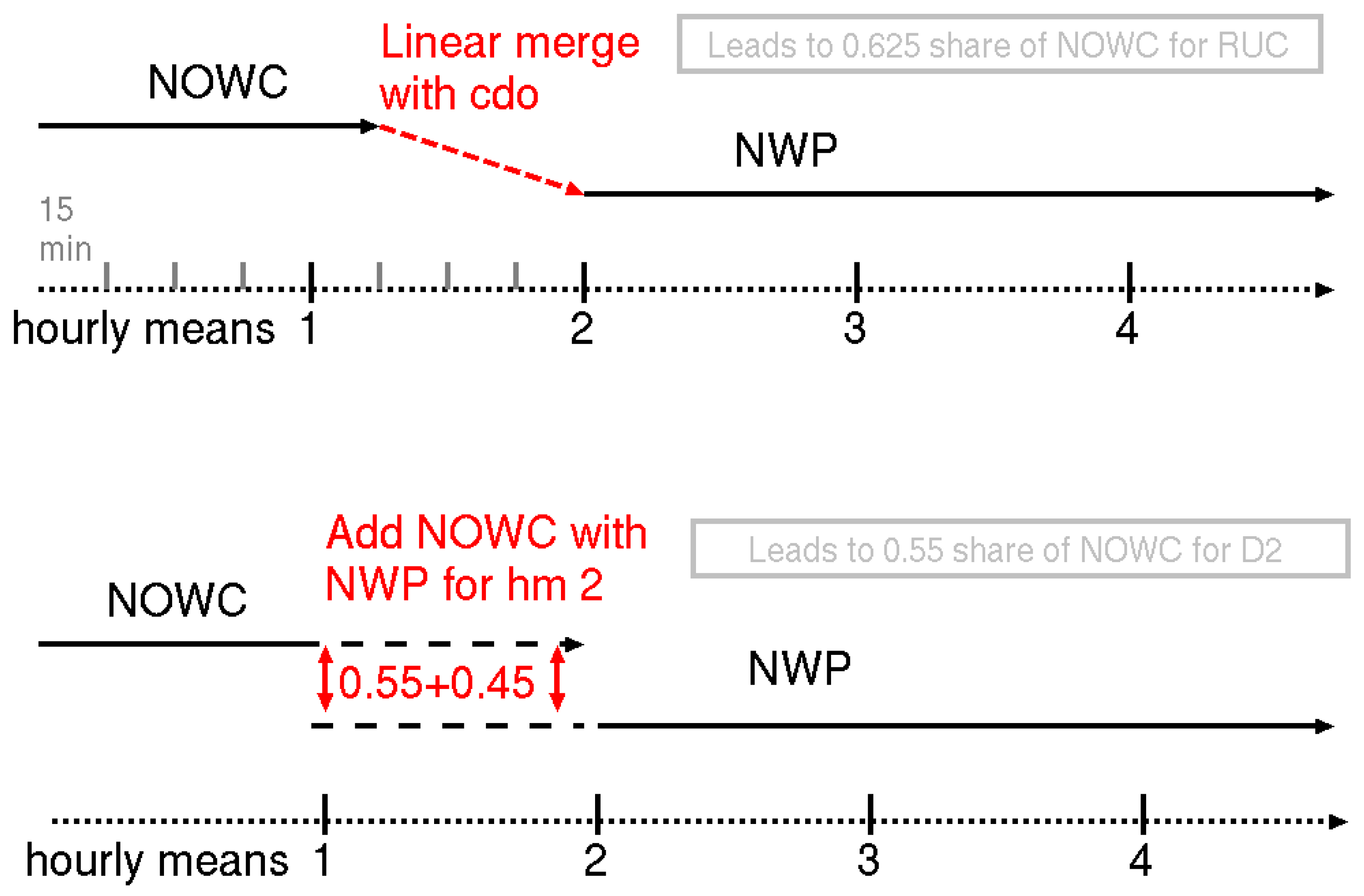
The closest available NWP runs in terms of time were used for the blending with the nowcast. As an example, for the blending taking place at 13 UTC, the most readily available ICON-D2 run is that of 9 UTC, as ICON-D2 takes 2 h to calculate and new runs only start every 3 h, so the 12 UTC run is not completed and no earlier run than that of 09 UTC is available. In contrast, the 12 UTC run of ICON-RUC is already available as a new run starts every hour and the calculation time is only 1 h for RUC. For the 14 UTC prediction, the 12 UTC run of ICON-D2 is ready; hence, the 12 UTC ICON-D2 run can be used. However, for RUC, the 13 UTC run is already ready and can be used. In the first step, the blending of the nowcasting and NWP was done as illustrated in Figure 5. For D2, this was done based on hourly values. In this case, "hourly" means that the nowcasting has been calculated beforehand. For RUC, the 15 min values were blended. However, in order to enable a comparison with D2, the hourly values of the blended product were calculated after blending. Because of the different time resolutions of RUC and D2, different blending methods were used; see Figure 5 for further details. For both approaches, the climate data operators were used [47].

Please note that the blended product is calculated every hour for the complete forecast horizon of 6 h.

3. Results

The data fusion of nowcasting and ICON was done in a pre-operational environment. As a result, RUC shows data gaps. Only time steps are used in the validation where both RUC and D2 were available.

For the statistical analysis of the forecasts (up to 6 h), established skill scores are used. In detail, these are the probability of detection (POD), the false alarm ratio (FAR) and the critical success index (CSI) [15,27,48]. These skill scores are based on 2 × 2 contingency tables [49] and are determined by the comparison of the predicted thunderstorms to the measured lightning. For the definition of hits, missed detections or false alarms, an object-based [48] or pixel-based approach is possible. Validation based on objects is not optimal to consider the size of the Cbs for the evaluation of the scores. This is why the pixel-based and object-based approaches are combined.

In order to avoid being overly strict with regard to the spatial uncertainties of the forecasts, a distance of 0.3 degrees between the combined forecast product and the lightning measurements is accepted and counted as an intersect. This distance of 0.3 degrees considers also the recommendations of the American Air Safety Authority, according to which aircraft should keep a lateral distance of 20 miles from thunderstorms. A hit is counted when lightning occurs within the search radius of a predicted thunderstorm; otherwise, it is counted as a false alarm. Thunderstorms are defined as missed if lightning occurs but no thunderstorm is predicted within the search radius of 0.3 degrees. The skill scores are calculated for each time step (1–6 h). The evaluation period covers May to September 2023.

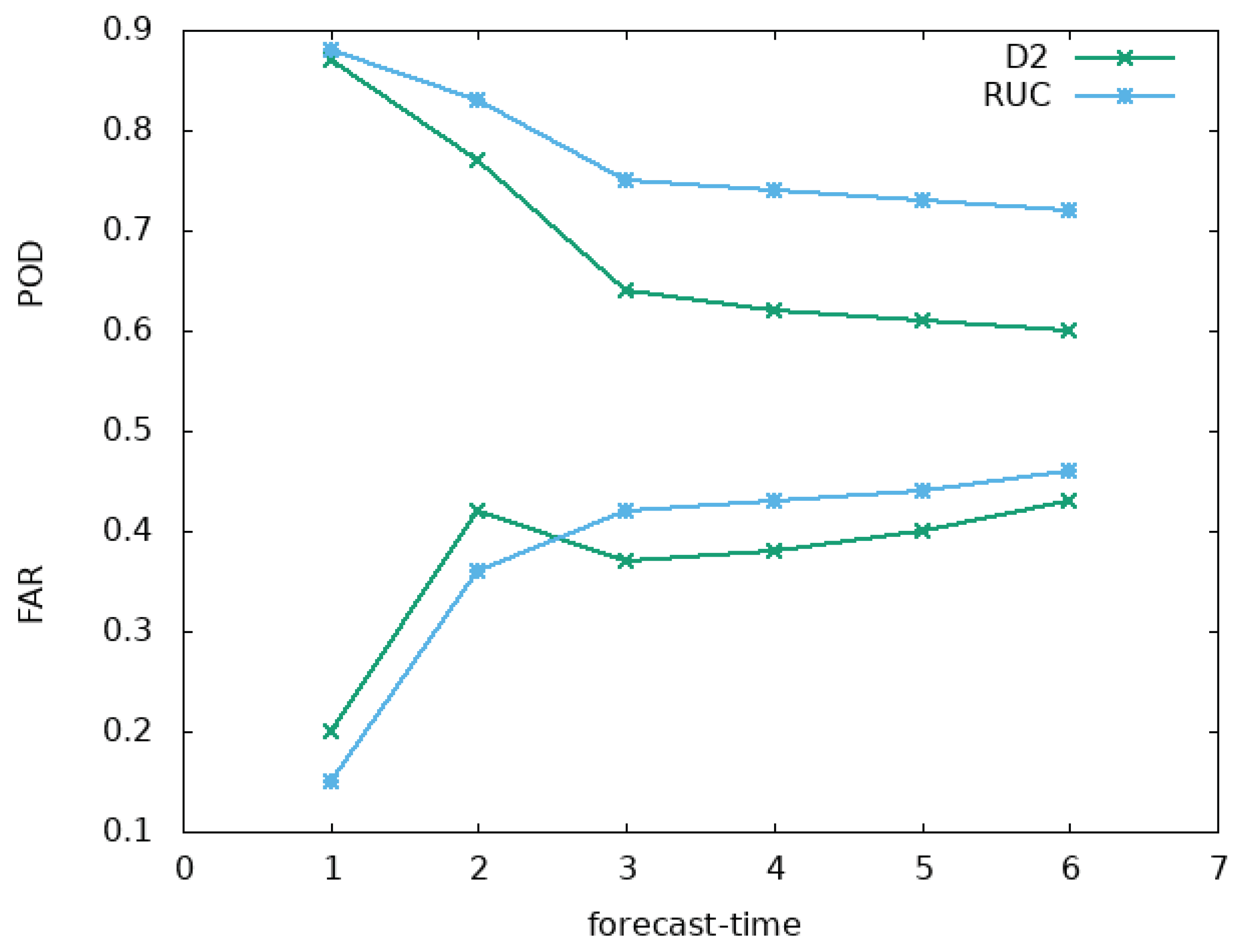
Figure 6 shows the results for CSI and Figure 7 for POD and FAR. The validation results indicate that the blended RUC product performs significantly better for the transition between NWP and nowcast, but also for the model-only forecast time steps.

The POD is higher throughout all time steps for the blended RUC product. The FAR for the blended D2 product shows a remarkable feature. It is higher for the nowcasting and blending step, but lower than RUC for the model-only forecast times. The reason for this lies in the poorer performance of the hourly atmospheric motion vectors compared to the 15 min values, which were used for the nowcasting and blending with RUC. Deviations from the linear movements of the cells within the hourly time steps are not well represented by the hourly mean AMV values, but much better with the 15 min resolution applied for the blending with RUC. Thus, on average, the movement of cells is much poorer for the blending with D2 than for the blending with RUC. Of course, this has no effect for the model-only time steps, as the internal calculation steps are identical for ICON-D2 and ICON-RUC. For the model-only steps (forecast times 3–6), the FAR of D2 is lower than that of RUC, but this cannot compensate for the significantly lower POD. Thus, the CSI is higher for RUC throughout all time steps.

However, what is the main driver of the significantly higher CSI of RUC for the model-only time steps? Is it due to the improved micro-physics or the higher assimilation rate? To address this question, the CSI is diagrammed over the lead time of the different model forecast steps in Figure 6. For this figure, the mean lead time is used for the time axis. For RUC, every hour, a new run with assimilation is started; hence, the lead time corresponds to the forecast time step given in Figure 6 plus 1 h. For ICON-D2, the average lead time is the forecast time step plus 3 h, as a result of the 3-hourly calculation interval and the 2-hourly calculation time. For illustration, the 11 UTC ICON-RUC model run is available for the blending starting at 12 UTC, but the closest available ICON-D2 run in terms of time is the 09 UTC run. Hence, for the respective 15 UTC forecast (3 h forecast time), the lead time for RUC is 3 + 1 h (11 to 15 UTC) and for D2 is 3 + 3 h (09 to 15 UTC). This results in the CSI over lead time as shown in Figure 8. Please note that, for this comparison only, the model-only time steps of the blended products were used.

The CSI applied over the lead time shows a linear transition between D2 and RUC. Thus, from this point of view, D2 and RUC perform equally. Thus, this is a clear indication that the main driver of the improvement in ICON-RUC is the higher data assimilation rate and not the improved micro-physics. In other words, the accuracy is data-driven. The differences in FAR and POD are induced by the slightly lower threshold of the LPI for D2 and RUC. The consequences will be further discussed in the next section.

The blended products were also analyzed visually with DWD’s meteorological workstation, NinJo [50]. Special focus was given to the transition between JuliaTSnow and the ICON model. The impression of the validation results could be verified. With ICON-RUC, a more seamless transition and thus prediction of thunderstorms is possible. Nevertheless, due to the chaotic nature of thunderstorms, inhomogeneities regularly occur with regard to the regional location and distribution of thunderstorms in the transition phase. However, it is probably not reasonable to artificially smooth the transition, as this would also remove the information indicating that there is an error in the NWP forecast.

The study of Urbich [28] provides evidence that the calculation of AMVs is less accurate with Farnebäck than with TV-L1 when validating for all cloud types [28]. Nevertheless, for thunderstorms, the method seems reliable enough as no significantly lower skill scores are apparent in comparison to NCS-A. The CTH product was evaluated by NCS-A users, namely pilots, in their daily praxis and has proven its worth.

The work presented here resulted in different new products, which are summarized in the following

Table 2. Overview of the novel DWD thunderstorm products. The temporal resolution is 15 min for CTH and JuliaTSnow and 1 h for the blended products. The spatial resolution corresponds to that of the satellite and is equal to or less than 0.05 for all products. Please note that the respective entries in the table are given for hourly values. For TS forecasts with higher temporal resolutions, the CSI would drop earlier, e.g., the CSI drops below 0.5 for JuliaTSnow roughly after 90 min if validation is performed for 15 min intervals.

Variable	Name	Availability	Coverage	Duration	Duration
				of Forecast	until CSI < 0.5
CTH	JuliaCTH	open data	Europe	0–90 min	n/a
TS	JuliaTSnow	open data	Europe, Africa	0–90 min	2 h
TS	blended	tbd	Central	0–6 h	3 h
	RUC		Europe
TS	blended	processing	Central	0–6 h	2 h
	D2	ended	Europe

. Please note that, after the evaluation of ICON-RUC, it was decided to move it to the 24/7 operational service. This enabled us to generate a 24/7 blended product with RUC and hence the processing of the blended D2 product was stopped.

The comparison of the duration until the CSI is below 0.5 demonstrates the value of RUC. With RUC, it is possible to extend the reliable nowcasting by up to 3 h for a given spatial uncertainty of less than 0.3 degrees, which would be not possible with AMV-based nowcasting alone.

4. Discussion

The results indicate that the higher CSI scores of ICON-RUC are mainly due to the faster update cycle of the data assimilation. This is supported by the theory of Lorenz [42] and well-established knowledge about chaos theory. Within this context, it is well known that the model errors increase rapidly at convection-permitting scales [51]. This explains why the information from the observations is rapidly lost. It is therefore obvious that a faster update cycle in data assimilation and the more accurate definition of the initial state of the atmosphere are the main drivers of the improvement in the NWP model-based 0–6 h predictions. Inconsistencies in the model physics could amplify these effects.

For these reasons, a central question arises: would it be better to carry out deep learning if the accuracy of the model system is determined by observations anyway and the NNP could devalue useful observations? In other words, would it be better to allow the network learn to the physics from the observations? Indeed, the results of deep learning provided in Brodehl et al. [33] indicate that higher skill scores without any model physics can be achieved for short-term forecasting than with state-of-the-art NWP models. Moreover, for other model parameters and medium-term forecasts, it has been shown that artificial intelligence can surpass NWP [52,53]. Of course, reanalysis data will continue to be very important, as reanalysis provides a consistent and rectified 4D data cube for the training of AI. However, what is the future of numerical weather prediction?

It is likely that numerical weather prediction in its current form will be replaced by data-driven AI models, within the ongoing AI revolution [54]. However, until then, it is important that data assimilation is improved. In addition to rapid updates of the assimilation, a description of the initial state that is as complete as possible is also extremely important. In the case of thunderstorm forecasts, the description of the initial state, and thus the ICON forecasts, could be improved by the assimilation of lightning data, e.g., [55].

However, the training of AI is not a trivial task and needs manpower and computing power. Further, regular retraining is needed. For this purpose, appropriate infrastructure, concerning both computer hardware and human resources, is needed. Some renowned European weather services are currently in a transitional phase, as both the computer infrastructure and staff are not optimally suited for AI. It is known from the social sciences that fundamental changes meet with resistance and that people have a tendency to adhere to the old ways. On one hand, this constitutes protection against hasty changes, but it can also slow down innovation and necessary changes. Applied to weather services, this could mean that NWP enthusiasts adhere to numerical weather prediction for too long. However, customers are likely not interested in the underlying method but in the quality of the products and services. Thus, it could be that many products and services associated with traditional weather services will become obsolete if they resist the AI revolution [54].

5. Conclusions

The blending of nowcasting with RUC shows higher CSI scores throughout the forecast horizon of 0–6 h. A faster update cycle for the calculation of the atmospheric motion vectors (AMVs) improves the temporal extrapolation of thunderstorms, which affects the CSI in the first two forecast hours. From the 3 h forecast onward, only model information is used in the blended product. The higher CSI for this prediction time demonstrates that ICON-RUC outperforms ICON-D2. However, the main advantage of RUC is given by the rapid update cycle, which forces the model to return to the reality more often. The results confirm that RUC enables a smooth transition from observation-based nowcasting to modeling. However, even with the rapid update cycle, the CSI drops below the critical value of 0.5 for the 3 h forecasts. Values below 0.5 mean that the number of hits (correct information) is lower than the number of failures, which result from missed cells plus false alarms. The product is then no longer useful in forecasting thunderstorms with spatial accuracy of 0.3 degrees. Compared to AI-based nowcasting [33,53], it seems that the ICON model loses the information contained in the observations quite rapidly. Thus, a solution to improve thunderstorm prediction in the 2–6 h range and to achieve CSI values higher than 0.5 could be a purely data-driven solution using artificial intelligence [56].