1. Introduction
The ENSO phenomenon in the Pacific Ocean has significant social and economic influence worldwide due to its global impacts on atmospheric and oceanic circulation and on marine and terrestrial ecosystems [
1]. The scale and magnitude of the hydrometeorological anomalies associated with El Niño and La Niña events make ENSO a major driver of global interannual climate variability [
2]. ENSO affects regions very distant from the tropical Pacific Ocean through nonstationary atmospheric teleconnections [
3].
In Ref. [
4], the teleconnections between the ENSO surface temperature and precipitation in the historical experiment and shared socioeconomic pathways (SSPs) of the CMIP6 [
5] were compared. Significant future (2081–2100) changes in ENSO precipitation teleconnections are expected relative to the changes during 1950–2014. In SSP experiments, the sea surface temperature (SST) variability increased in most CMIP6 models, but to varying degrees [
6].
A wide range of projections was shown for the ENSO amplitude in the CMIP5 (the previous phase of the CMIP) and CMIP6 models by the end of the 21st century, from an increase in the standard deviation of up to +0.6 °C to a decrease in the standard deviation to −0.4 °C [
7]. However, despite the large inter-model variability in ENSO-related SST anomalies, the model results have documented a persistent intensification and eastward shift of ENSO-induced precipitation under global warming [
8].
There are persistent interdecadal variations in the intensity and location of major anomalies in El Niño and La Niña events, which are associated with disturbances in the wind and the thermocline depth at the equator, as well as extratropical anomalies in the north and south Pacific [
9].
An important aspect of the ENSO phenomenon is the asymmetry between its two opposing phases: El Niño and La Niña. An assessment of the reproduction of this ENSO property using CMIP6 models shows that models continue to underestimate this asymmetry [
10]. Another important feature of ENSO is the presence of two types of events: the east Pacific (EP) and central Pacific (CP) events. CMIP6 models reproduce the amplitude and spatial structure of CP ENSO better compared to CMIP5 models [
11].
The authors of [
12] estimated the seasonal phase synchronization of ENSO using 42 CMIP6 models, 43 CMIP5 models, and observational data. Only a few models (12 CMIP5 and 15 CMIP6 models) reproduced ENSO with a higher proportion of winter peak events, indicating that the seasonal synchronization of ENSO phases is still a challenge for current climate models. Thus, most CMIP5 and CMIP6 models failed to reproduce the phase synchronization of ENSO because the contribution of zonal advective feedback to the seasonal modulation of the SST growth rate was much smaller compared to the observations [
13,
14]. In addition, no consistent relationships were found between changes in the annual cycle and the ENSO amplitude in paleoclimate experiments with CMIP5/6 models [
15].
ENSO interacts with the Indian Ocean dipole (IOD), necessitating the simultaneous modeling of ENSO and the IOD. ENSO and the IOD are linked through the Walker circulation, which connects the Pacific and Indian Oceans. Given the pronounced impact of ENSO and the IOD on the global and regional climate, their accurate representation in climate models is crucial for producing reliable climate projections. By using 32 CMIP5 and 34 CMIP6 models, the authors of [
16] found that there were changes in the main characteristics of ENSO and the IOD in CMIP6 models compared to CMIP5 models. Most CMIP6 models can reproduce the leading dipole mode of heat content anomalies between the east and west tropical Indian Ocean, but they largely overestimate the amplitude and dominant period of the subsurface IOD [
17].
The Walker circulation is a major component of the global climate system. It links the variability in the surface temperature of the Pacific Ocean with the climate variability in other oceans up to the middle and high latitudes. However, the atmospheric feedback associated with ENSO, in particular the surface wind response, is largely underestimated in CMIP5/6 models. Differences in the SLP and the Walker circulation characteristics between different models have also been identified. While the SLP responses to ENSO-related SST variability are well reproduced in most models, the Walker circulation streamfunction responses are largely underestimated in most of these models [
18].
Some ENSO precursors are associated with the north Pacific oscillation (NPO): the trade wind charging (TWC) of the subsurface heat content at the equator of the Pacific Ocean and the northern Pacific meridional mode (NPMM) [
19]. In [
20], whether the TWC/NPMM regime and its relationship with ENSO are reproduced in high-resolution CMIP6 models was assessed. The relationship between ENSO and the winter synoptic temperature variability over the Asia–Pacific–American region is reproduced in most CMIP5/6 models with significant differences from observational data [
21].
CMIP6 models can reproduce ENSO signals well in the Arctic stratosphere and have demonstrated an improved performance compared to CMIP5 models [
22]. In particular, El Niño events are associated with a strengthened Pacific–North American (PNA) pattern, which results in a warm and weakened stratospheric polar vortex. In addition, the response of the Arctic stratosphere to El Niño phenomena depends on their type: EP or CP [
23].
In references [
24,
25,
26,
27], an attempt to combine forward and backward teleconnections between ENSO and climate processes across the Earth into one planetary phenomenon called the global atmospheric oscillation (GAO) was made. An analysis of the global variations in the hydrometeorological parameters between opposite phases of ENSO in the general circulation models of the atmosphere and ocean that participated in the CMIP5 showed the reproduction of the planetary spatial structure of the GAO by some of the considered climate models [
28].
The authors of [
29] found that CMIP6 models significantly outperformed CMIP5 models for 8 out of 24 ENSO-related metrics, with most CMIP6 models showing improved tropical Pacific seasonality and ENSO teleconnections. In [
30], significant improvements in the representation of ENSO by CMIP6 models compared to CMIP5 models were revealed. In addition, the teleconnections of the total cloud fraction with the global SST in a CMIP6 multi-model ensemble performed better than those of a CMIP5 multi-model ensemble [
31].
In climatological research, the evaluation of climate models is one of the central research subjects. As an expression of large-scale dynamical processes, global teleconnections play a major role in the interannual-to-decadal climate variability. Their realistic representation is an indispensable requirement for the simulation of climate change, both natural and anthropogenic. Therefore, the evaluation of global teleconnections is of utmost importance when assessing the physical plausibility of climate projections [
32].
The purpose of this work was to investigate how CMIP6 models reproduce the main characteristics and teleconnections of ENSO. In addition, the main goals of this work were to identify the models that reproduced the strongest links between ENSO and the extratropics and to verify that the CMIP6 models reproduced the GAO’s planetary spatial structure of the ST and SLP anomaly oscillation amplitudes between El Niño and La Niña.
This paper is organized as follows. The “
Section 1” provides an overview of the existing works on the research topic. The “
Section 2” provides a description of the models and indices analyzed. The “
Section 3” contains a comparison of the ENSO teleconnection simulations. The “
Section 4” concludes the paper with a summary.
2. Materials and Methods
We examined global data on the ST (“skin” temperature, i.e., the SST for the open ocean) and the SLP (the atmospheric pressure with the effects of elevation removed) obtained as a result of the pre-industrial control (piControl) experiment on the atmosphere–ocean general circulation models included in the CMIP6 [
5]. The piControl experiment was chosen over the historical experiment because there was a significant temperature trend in the historical experiment. In the piControl experiment, there were no external forces affecting the changes in the concentration of greenhouse gases in the atmosphere and variations in solar radiation. Of the external forces influencing the climate system, only the annual variation in the heat input from the sun was present in the piControl experiment. At the same time, the coupled calculations of the atmosphere–ocean general circulation performed within the framework of the piControl experiment covered long periods (about 500 model years). All the subsequent analyses and averaging were performed on the piControl experimental results for the 50 CMIP6 models listed in
Table 1.
To determine El Niño and La Niña events, this work used an index called the oceanic Niño index (ONI). The ONI represents the average values of the SST anomalies in the Niño 3.4 region (5° N–5° S, 170°–120° W). The average annual cycle of the ST and SLP for each model over the entire period of the piControl experiment were calculated. The annual cycle was removed from each model’s ST and SLP data to obtain the ST and SLP anomalies. Then, the ST anomalies were averaged in the Niño 3.4 region (5° N–5° S, 170°–80° W), and the resulting time series was smoothed with a 3-month moving average to obtain a separate ONI for each model. Low-frequency changes were removed from the ONI time series using a 30-year Butterworth filter. Based on the obtained ONI, the El Niño and La Niña events were determined separately for each model. During El Niño (La Niña), the ONI values must continuously exceed +0.5 °C (less than −0.5 °C) for 5 months or more.
To evaluate the global ENSO teleconnections, the GAO1 index was used [
33], which was calculated as the sum of the normalized values of the SLP anomalies in 10 regions, coinciding with the maxima and minima in the spatial structure of the SLP anomalies of the GAO field [
34]. GAO1 was calculated using the following formula:
where P is the average value of SLP anomalies in the areas with given coordinates. The choice of sign (“+” or “−”) used for each region included in the GAO1 formula was related to the type of SLP anomalies (positive or negative) that are observed in the region during El Niño events.
To characterize the teleconnections of the tropics of the Pacific Ocean with other regions included in the planetary structure of the GAO, the components (5° S–5° N, 145°–155° E) and (5° S–5° N, 95°–85° W) were excluded from GAO1. Since the SLP anomalies in these areas are used to calculate the equatorial southern oscillation (SO) index, the GAO is thus separate from the SO [
33]. The GAO index without the SO was calculated based on the normalized SLP anomalies in eight regions using the following formula:
where P is the average value of SLP anomalies in the areas with given coordinates.
Then, to characterize the teleconnections of ENSO with extratropical latitudes, regions in the tropics of the Indian Ocean (5° S–5° N, 55°–65° E) and Atlantic Ocean (5° S–5° N, 35°–25° W) were excluded from the GAO2 index. The resulting GAO index was called the extratropical GAO index (EGAO) [
33]:
where P is the average value of SLP anomalies in the areas with given coordinates.
The average fields of the amplitude of oscillations of the ST and SLP anomalies between the opposite phases of ENSO were calculated using the ONI for each of the 50 CMIP6 models under consideration. Based on this, the average model fields were calculated and their inter-model variability was assessed using standard deviations.
The energy spectra of the ONI and the GAO index were estimated using the fast Fourier transform method with the maximum resolution [
33]. Each observation record of a hydrological quantity, even if that quantity was continuously changing, had a finite length and a finite temporal resolution. Such a record cannot be represented by the Fourier integral S(f) (f is a continuously varying frequency), but only by a finite series of Fourier coefficients S(f
n) (where f
n is from a discrete sequence of frequencies) corresponding to harmonics that are multiples of the total length of the record. As a result, the actual amplitude of a Fourier harmonic that is not a multiple of the total recording length may be underestimated if that amplitude differs significantly from the amplitudes of nearby harmonics. To avoid this, multiple periodogram calculations can be used for the records that remain after successive reductions in the initial record. Then, all such periodograms are combined, and if the periods coincide, they are averaged. This increases the spectral resolution, and thus, makes it possible to more accurately locate spectral density peaks at periods that are not a multiple of the total length of the original recording. Apparently, this technique was first used in [
35].
Using this method, power spectra were estimated not only for the total recording length, but also for the sequentially reduced time series, followed by combinations of all the resulting periodograms [
26,
33]. The maximum resolution spectra of the ONI and the GAO index were constructed by sequentially reducing the lengths of their time series to half their original length, since this produced the most continuous estimates of the spectral density for all frequencies. The spectra were first estimated for a series with a length of N: (1, …, N); then, they were estimated for two series with lengths of N − 1: (1, …, N − 1) and (2, …, N); then, they were estimated for three series with lengths of N − 2: (1, …, N − 2), (2, …, N − 1), and (3, …, N), etc.; and this continued up to N/2 series with lengths of N/2: (1, …, N/2), (2, …, N/2 + 1), …, (N/2, …, N). Next, all the obtained spectra were combined into one by ordering them according to their frequency and averaging when the frequencies matched. In this case, a spectral assessment of the indices was carried out on an annual period [
26,
33]. For this purpose, spectra with the maximum resolution of the indices were calculated for each month of the year separately. Then, the 12 spectra obtained for each index were averaged. This technique of spectral estimation on the period of an external force made it possible to reduce the influence of this periodicity on the resulting spectra.
3. Results and Discussion
The ONI standard deviation, averaged over 50 CMIP6 models, was 0.9 °C (
Table 1, column 5). The minimum standard deviation of the ONI was demonstrated by INM-CM4-8 (0.41 °C), and the maximum was demonstrated by CMCC-ESM2 (1.48 °C). The average minimum value of the ONI was −3.02 °C (
Table 1, column 6). The largest absolute minimum ONI value was shown by CAMS-CSM1-0 (−4.62 °C), and the smallest was shown by INM-CM4-8 (−1.48 °C). The average maximum value of the ONI was +3.24 °C (
Table 1, column 7). The highest maximum ONI value was shown by CMCC-CM2-SR5 (+4.85 °C), and the lowest was shown by INM-CM4-8 (+1.55 °C). Thus, INM-CM4-8 exhibited the weakest ONI variability out of the 50 CMIP6 models considered.
ENSO is characterized by an asymmetry, one of the features of which is higher absolute values of SST anomalies in the equatorial Pacific Ocean during the strongest El Niño events compared to those during the strongest La Niña events [
36]. This ENSO asymmetry was not observed in some of the 50 CMIP6 models considered. For some of the CMIP6 models, the minimum ONI values turned out to be greater in absolute value than the maximum ONI values (
Table 1).
The average ENSO period across the 50 CMIP6 models was 4.3 years (
Table 1, column 8). It was calculated for each model as twice the number of years of the experiment divided by the total number of El Niño and La Niña events. At the same time, the minimum average ENSO period was demonstrated by CAMS-CSM1-0 (2.86 years), and the maximum was demonstrated by INM-CM4-8 (11.54 years). The average duration of El Niño events across the 50 CMIP6 models was 12 months (
Table 1, column 9). At the same time, the minimum average duration of El Niño events was demonstrated by BCC-ESM1 (7.6 months), and the maximum was demonstrated by CMCC-ESM2 (18.4 months). The average duration of La Niña events across the 50 CMIP6 models was 12 months (
Table 1, column 10). At the same time, the minimum average duration of La Niña events was demonstrated by INM-CM4-8 (7.5 months), and the maximum was demonstrated by MIROC-ES2L (19.5 months). INM-CM4-8 exhibited a long average period between ENSO events, as well as a short average duration of El Niño and La Niña events, due to the low ONI variability noted above, which is why the event-selection criterion (0.5 °C) rarely worked.
Some CMIP6 models showed longer average durations for El Niño events than for La Niña events (
Table 1). This asymmetry in the duration of ENSO events is opposite to the results obtained from observational data. Thus, during the period of reliable instrumental observations (1950–2022), the La Niña events (1954–1956, 1998–2001, etc.) continued for longer than any of the El Niño events recorded during this period [
37].
Thus, it can be concluded that there are differences in the main characteristics of ENSO among the CMIP6 models (minimum, maximum, and standard deviation values shown in
Table 1). Moreover, some of the considered CMIP6 models reproduced the main characteristics of ENSO and the asymmetry between the El Niño and La Niña events with differences from those observed using instrumental measurements. Based on this, we can conclude that not all CMIP6 models satisfactorily reproduce the basic characteristics of ENSO.
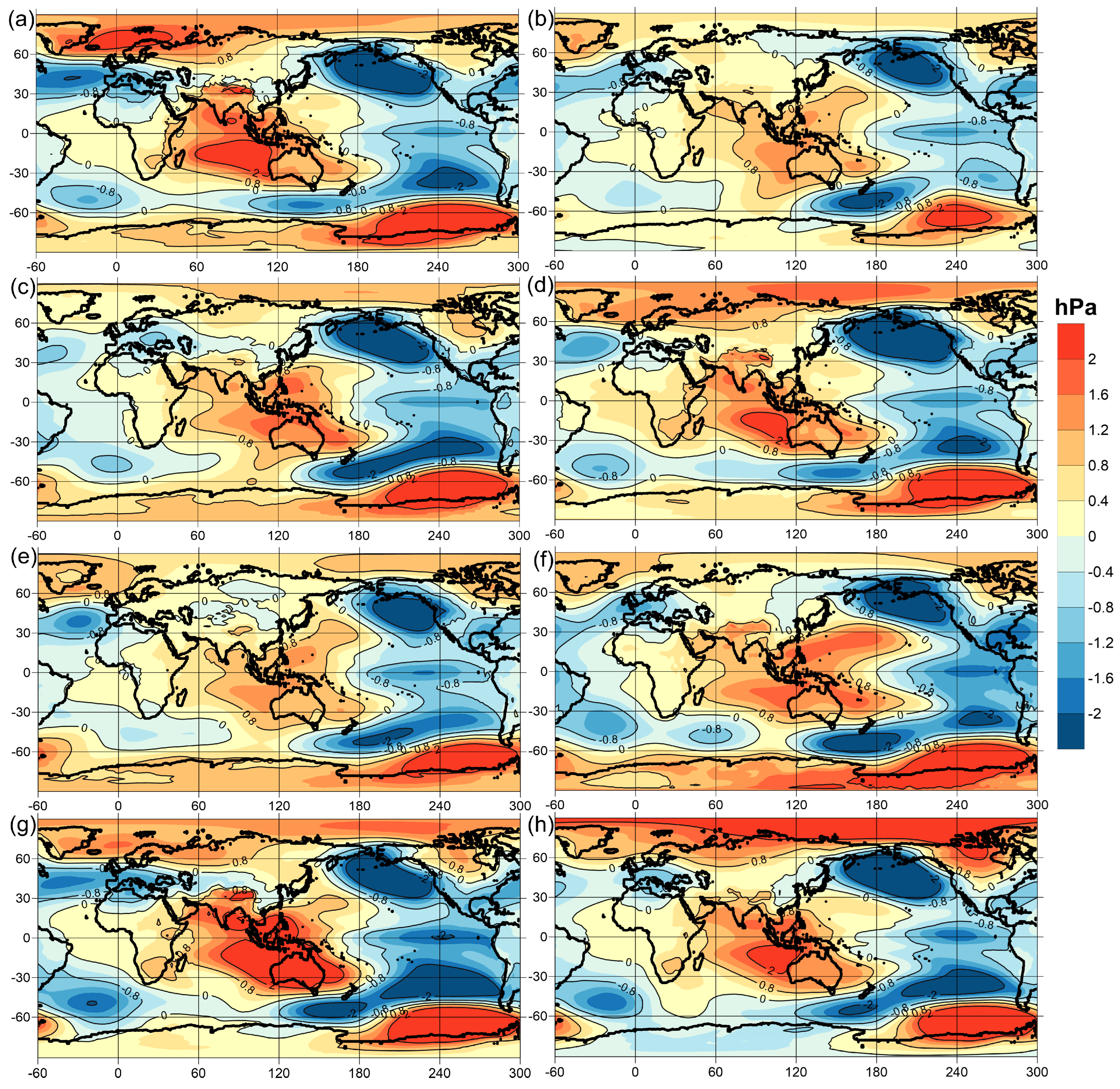
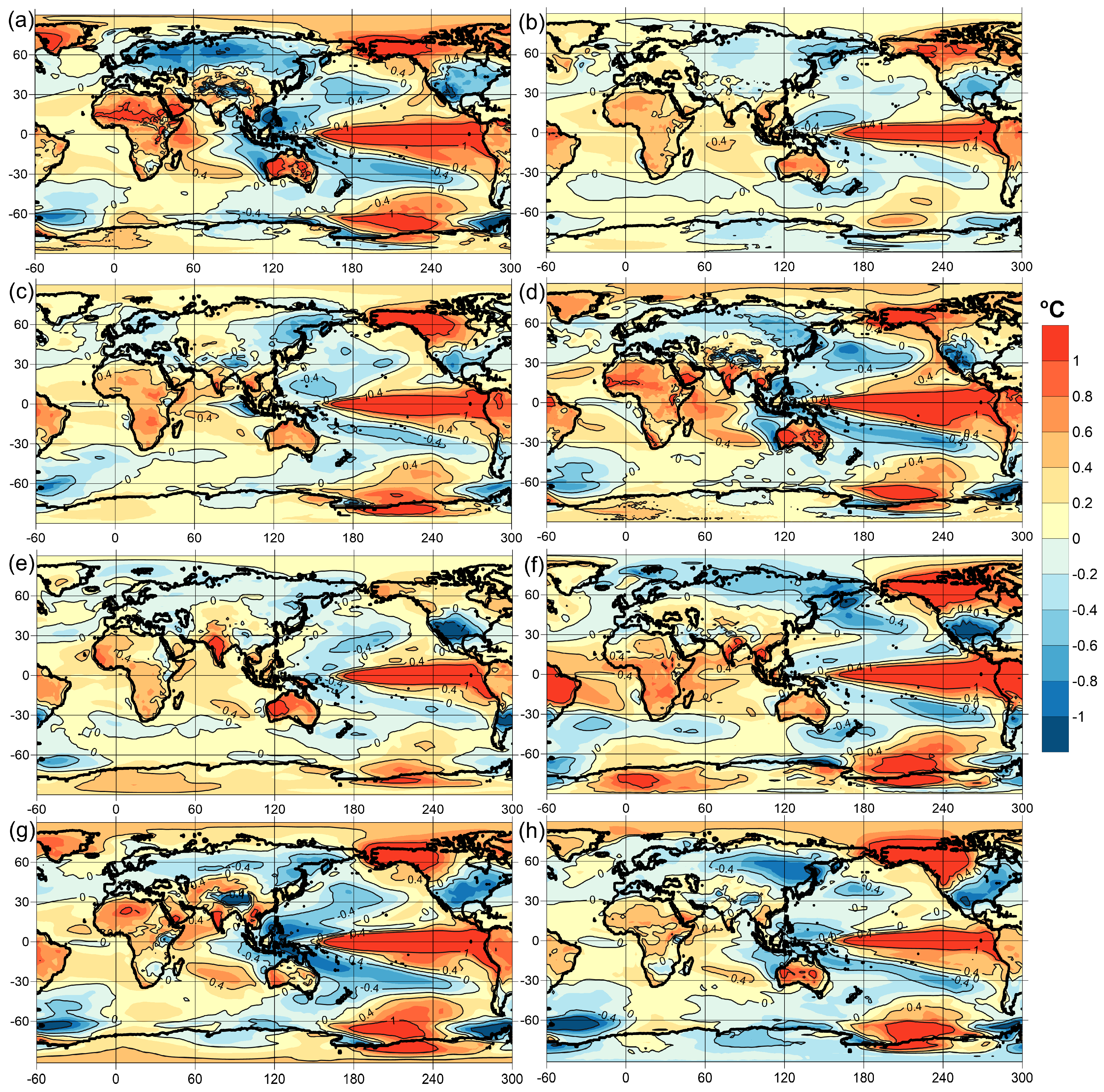
Figure 1 shows the amplitude fields of the fluctuations in the mean ST anomalies between opposite ENSO phases for 8 of the 50 CMIP6 models, constructed using the ONI using the method described in the
Section 2. These eight models were chosen based on their reproduction of the strong teleconnections of ENSO with regions beyond the tropical Pacific. The fields for the other 42 models are presented in the
Supplementary Materials. It is noteworthy that a large proportion of these models reproduced the global spatial structure of the amplitude of the ST anomaly oscillations quite well between El Niño and La Niña (GAO ST field) [
24,
25,
34,
38]. The GAO ST field is symmetrical relative to the equator, taking into account the location of the continents. Moreover, compared to the CMIP5 models [
28], the number of CMIP6 models that reproduced the GAO ST field increased. Thus, it can be concluded that the CMIP6 models resulted in an improved description of the teleconnections between ENSO and the ST outside the tropical Pacific compared to the CMIP5 models.
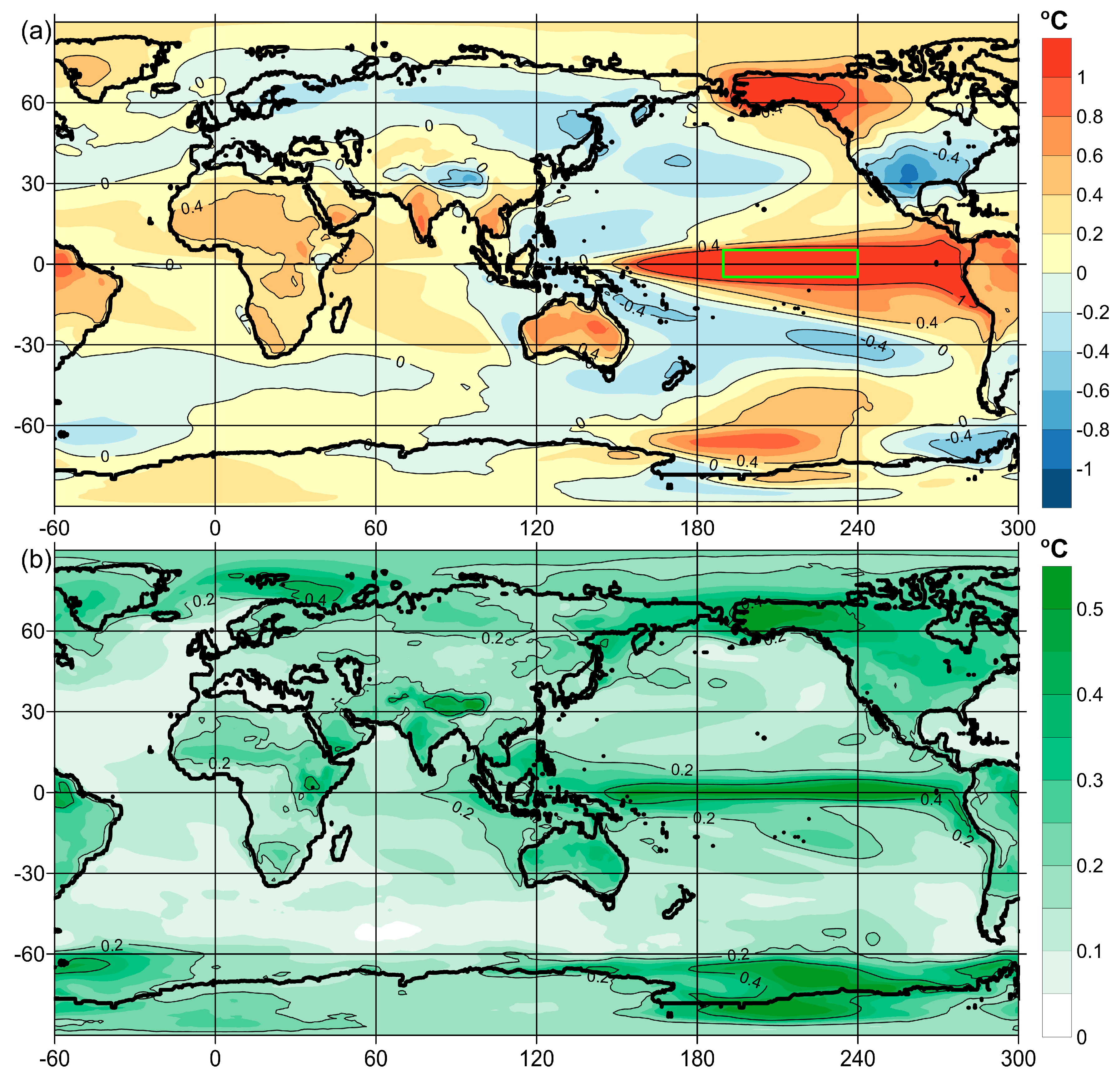
Additionally, an amplitude field of the fluctuations in the mean ST anomalies between opposite ENSO phases, averaged over the 50 CMIP6 models considered, was constructed (
Figure 2a). To achieve this, the GAO ST fields obtained for each of the 50 CMIP6 models were interpolated onto a single 1° × 1° grid and then averaged among themselves. The GAO ST field averaged for 50 CMIP6 models contained many of the same details as the GAO ST fields obtained previously from observational data and reanalyses [
24,
25,
34,
38]. In the GAO ST field averaged over 50 CMIP6 models, characteristic positive ST anomalies for El Niño were observed along the equator of the central and eastern Pacific Ocean—the so-called “tongue” of positive SST anomalies. Weaker values of positive ST anomalies extended from the equator north and south along the coasts of North and South America. Upon reaching high latitudes, they intensified and formed two positive ST anomalies located symmetrically relative to the equator over Alaska and the Amundsen and Ross Seas. Weaker positive ST anomalies extended further into the polar regions up to Greenland and Antarctica, but their magnitudes were small and their inter-model variability was high (
Figure 2b). The inter-model variability, represented by the standard deviation, was also high at the Pacific equator, indicating differences in the CMIP6 models’ reproduction of typical ENSO SST anomalies in this region.
In the GAO ST field averaged over 50 CMIP6 models, negative anomalies were located in the western Pacific Ocean, with two centers in the mid-latitudes of its northern and southern parts (
Figure 2a). From these regions, negative ST anomalies spread to northern Eurasia and the region south of Australia, but their magnitude was small. Negative ST anomalies were also observed in central North America and south of South America. Thus, negative ST anomalies partially surrounded the region of the tropics of the Indian and Atlantic Oceans, which was covered predominantly by positive ST anomalies, including the Hindustan Peninsula, Southeast Asia, part of the Indonesian archipelago, Australia, Africa, and the Arabian Peninsula. An exception is the region of the Himalayas and the Tibetan Plateau, where, apparently due to the high altitude above sea level, negative ST anomalies were located.
In the GAO ST field averaged over 50 CMIP6 models (
Figure 2a) and the field of its standard deviations among 50 CMIP6 models (
Figure 2b), it is noteworthy that large absolute values of ST anomalies were observed, both over the oceans and over continents, but over land, the inter-model variability was usually higher (about 0.2 °C). The exceptions were the equatorial region of the Pacific Ocean, where El Niño and La Niña events develop, as well as the waters of the Southern and Arctic Oceans, which are covered with ice most of the year. Thus, the spatial structure of the GAO ST field was more stable over the oceans than over the continents, which indicates the significant role of the interaction between the atmosphere and the ocean in its formation, and, accordingly, in the formation of extratropical ENSO teleconnections.
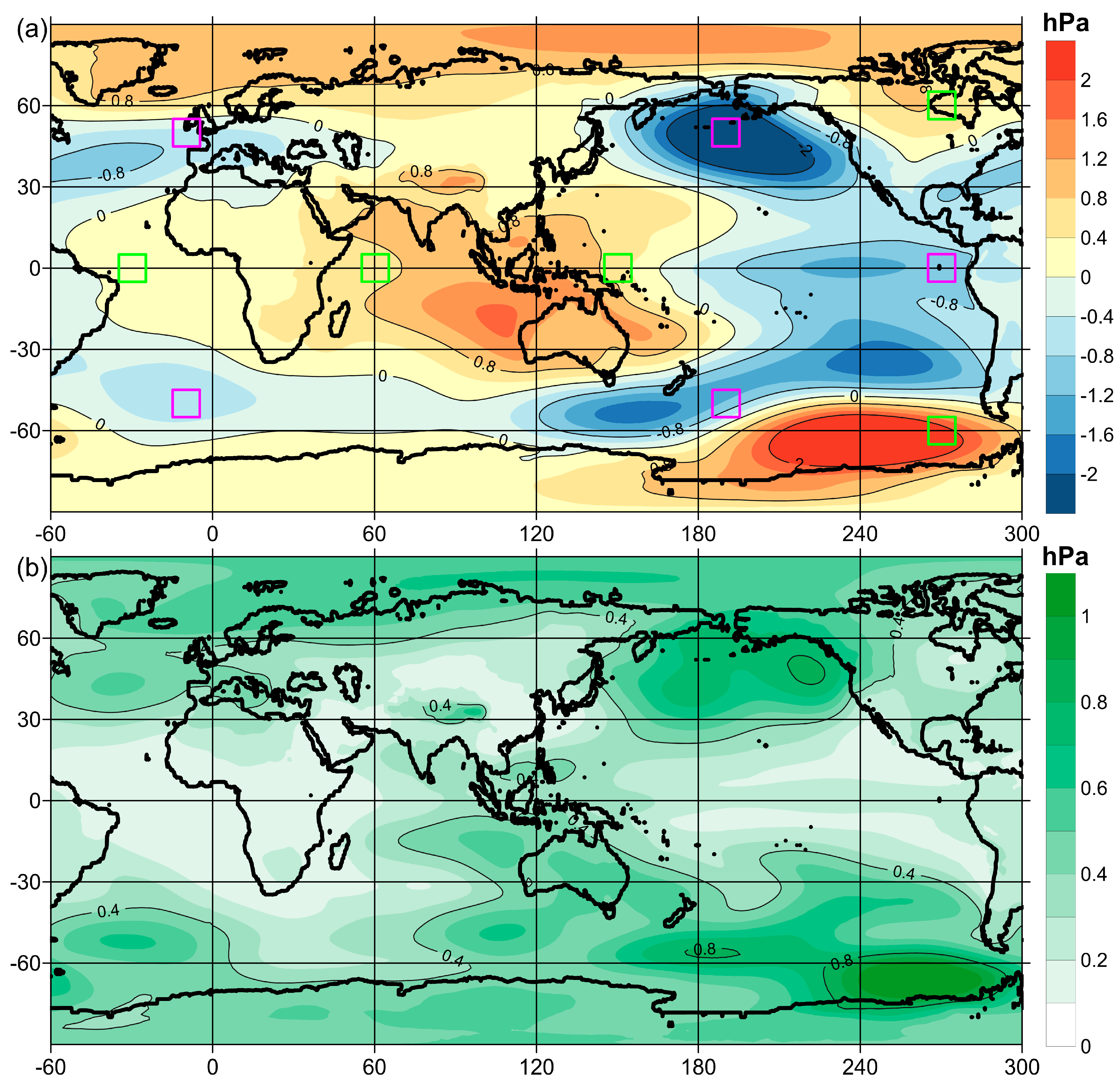
Let us consider the global structure of the amplitude of oscillations of SLP anomalies between opposite phases of ENSO (GAO SLP field) for the CMIP6 models separately (
Figure 3 and
Supplementary Materials) and the average of all 50 models under consideration (
Figure 4a). In reference [
28], GAO SLP fields were constructed for most of the CMIP5 models. It turned out that only a minority of the CMIP5 models reproduced the GAO SLP field obtained previously from observational data [
24,
25,
34,
38]. In the CMIP6, the number of models that reproduced the features of the planetary structure of the GAO SLP field increased compared to the CMIP5 models [
28]. The global spatial structure of the GAO SLP field had symmetry relative to the equator (
Figure 4a), just like the GAO ST field (
Figure 2a). Moreover, the GAO SLP field also had symmetry relative to 90° W, taking into account the configuration of the continents.
The GAO SLP field was characterized by an X-shaped structure of negative SLP anomalies, with a crosshair at the equator of the Pacific Ocean in the region of 90° W (
Figure 3 and
Figure 4a) [
24,
25,
34,
38]. From this crosshair, rays of negative SLP anomalies diverged in four directions: to the northwest up to the Chukotka Peninsula, to the northeast up to Europe, and to the southwest and southeast up to Antarctica. These rays of negative SLP anomalies covered a large ellipse-shaped region of positive SLP anomalies centered on the equator of the Indian Ocean. It should be noted that the rays of negative SLP anomalies were closed only in the Southern Hemisphere, and this closure occurred over the ocean. In the Northern Hemisphere, there was a gap between the rays of negative SLP anomalies over the Asian continent. Apparently, this feature was associated with the important role of the interaction between the atmosphere and the ocean in the formation of the planetary structure of the GAO SLP field.
In the high latitudes north and south of the crosshairs of the rays of negative SLP anomalies at (0° lat., 90° W), there were regions from which positive SLP anomalies occurred and spread into the Arctic and Antarctic. Given the large magnitude of the SLP anomalies at high latitudes (more than 0.8 hPa), their inter-model variability was also very large (about 0.5 hPa) (
Figure 4b). The lowest inter-model variability in the SLP anomalies was observed over the oceans in the tropics (about 0.1 hPa), which further indicates the importance of atmosphere–ocean interaction processes in the formation of the spatial structure of the GAO SLP field and ENSO teleconnections.
It is noteworthy that, of the 50 CMIP6 models considered, the models that better reproduced the spatial structure of the GAO SLP field were also the same models that reproduced the spatial structure of the GAO ST field well. Thus, we concluded that the planetary spatial structures of the GAO ST and GAO SLP fields are interconnected. Moreover, the models that reproduced the planetary spatial structures of the GAO ST and GAO SLP fields described the ENSO teleconnections well. Thanks to this, these models could also reproduce the teleconnections between ENSO and other hydrometeorological parameters, such as the ocean temperature at various depths [
26], precipitation, wind, and air humidity [
38], with a higher accuracy. However, an analysis of the CMIP6 models’ reproduction of ENSO teleconnections with hydrometeorological parameters other than the ST and SLP requires a separate study.
To assess the presence in the CMIP6 models of ENSO teleconnections with hydrometeorological parameters outside the tropics of the Pacific Ocean, an asynchronous cross-correlation analysis method was applied between the ONI and the three GAO indices defined in the
Section 2—GAO1, GAO2, and EGAO (
Table 2). The GAO1 index characterizes the entire planetary structure of the GAO SLP field, the tropics of the Pacific Ocean are excluded from the GAO2 index, and the entire tropical belt of the Earth is excluded from the EGAO index.
Table 2 presents the average periods of fluctuations between opposite phases of the GAO1, GAO2, and EGAO indices, which were selected as for ONI based on the 0.5 criterion. The average period of oscillations was calculated as twice the number of years of the experiment divided by the total number of positive and negative phases of a given GAO index. The average model fluctuation periods turned out to be 3.96 years for GAO1, 4.39 years for GAO2, and 4.81 years for EGAO (
Table 2; columns 2, 5, and 8). The average model periods for the GAO indices turned out to be close to the average model period for the ONI (4.3 years). Moreover, the average period of the GAO1 index was less than the period for the GAO2 index, which, in turn, was less than the period for the EGAO index. It follows from this that the exclusion of the tropical part from the GAO indices increased the average period of oscillation for the remaining part of the GAO.
Cross-correlations between the ONI and the GAO index were calculated in 1-month increments with shifts from −60 to +60 months after bandpass-filtering their time series from 2 to 7 years. The maximum absolute values of correlations (
Table 2; columns 3, 6, and 9) and the shifts to which they corresponded were determined. If the maximum correlation shift indicated in
Table 2 (columns 4, 7, and 10) is positive, this means that the ONI was ahead of the GAO index; if it is negative, it means the ONI lagged behind the GAO index. Almost all the models demonstrated high correlations between the ONI and GAO1—the average correlation was 0.89 (
Table 2, column 3). This was expected, since GAO1 includes regions in the tropical Pacific Ocean from which the equatorial southern oscillation index was calculated. At the same time, the minimum correlation between the EONI and GAO1 among all 50 CMIP6 models considered was observed in the INM-CM5-0 model (0.67), and the maximum was observed in the CESM2-WACCM-FV2 model (0.96).
With the tropical Pacific excluded, the correlation values between the GAO2 index and the ONI were smaller than those between GAO1 and the ONI—the average correlation was 0.76 (
Table 2, column 6). The minimum correlation between the ONI and GAO2 among all 50 CMIP6 models considered was observed for the INM-CM5-0 model (0.47), and the maximum was observed for the CESM2-WACCM-FV2 model (0.91). The shifts at which the maximum correlations between GAO1 and GAO2 with the ONI were observed were close to 0 for all 50 models, indicating that GAO1 and GAO2 vary synchronously with the ONI.
For the EGAO index, from which the entire tropical belt of the Earth was excluded, the correlation values between it and the ONI became even smaller compared to those of previous indices—the average correlation was 0.61 (
Table 2, column 9). The minimum correlation between the ONI and EGAO among all 50 CMIP6 models considered was observed for the INM-CM4-8 and INM-CM5-0 models (0.3), and the maximum was observed for the CESM2-WACCM-FV2 model (0.88). Thus, after the low latitudes were removed from the GAO, the magnitude of the teleconnections of its remaining part with ENSO decreased and the inter-model variability in these teleconnections increased (average and standard deviation values in
Table 2). However, there was a slight lag (1–2 months) of the EGAO relative to the ONI, indicating that the extratropical spatial structure of the GAO SLP field (
Figure 4a) was associated with the response to El Niño and La Niña events caused by global ENSO teleconnections (
Table 2, column 10).
In addition to the planetary structure of teleconnections, ENSO is characterized by the temporal dynamics that are characteristic of a strange non-chaotic attractor (SNA) [
33]. In an SNA, a nonlinear dynamic system is affected by two or more external quasi-periodic forces with incommensurate oscillation frequencies. The ratio of their periods is very poorly approximated by rational numbers. One example of such a ratio between periods is the golden ratio and its linear transformations. Due to the incommensurability of their periods, external forces act on the system as if at random, and the system’s behavior seems random, although, in fact, it is non-chaotic. Spectral estimates of the characteristics (indices) of such a system demonstrated peaks at frequencies that were all possible combinations of periods of external forces acting on the system. Due to this, such spectra appeared continuous, although they consisted of a countable number of peaks, between which there were frequencies with zero oscillation energies.
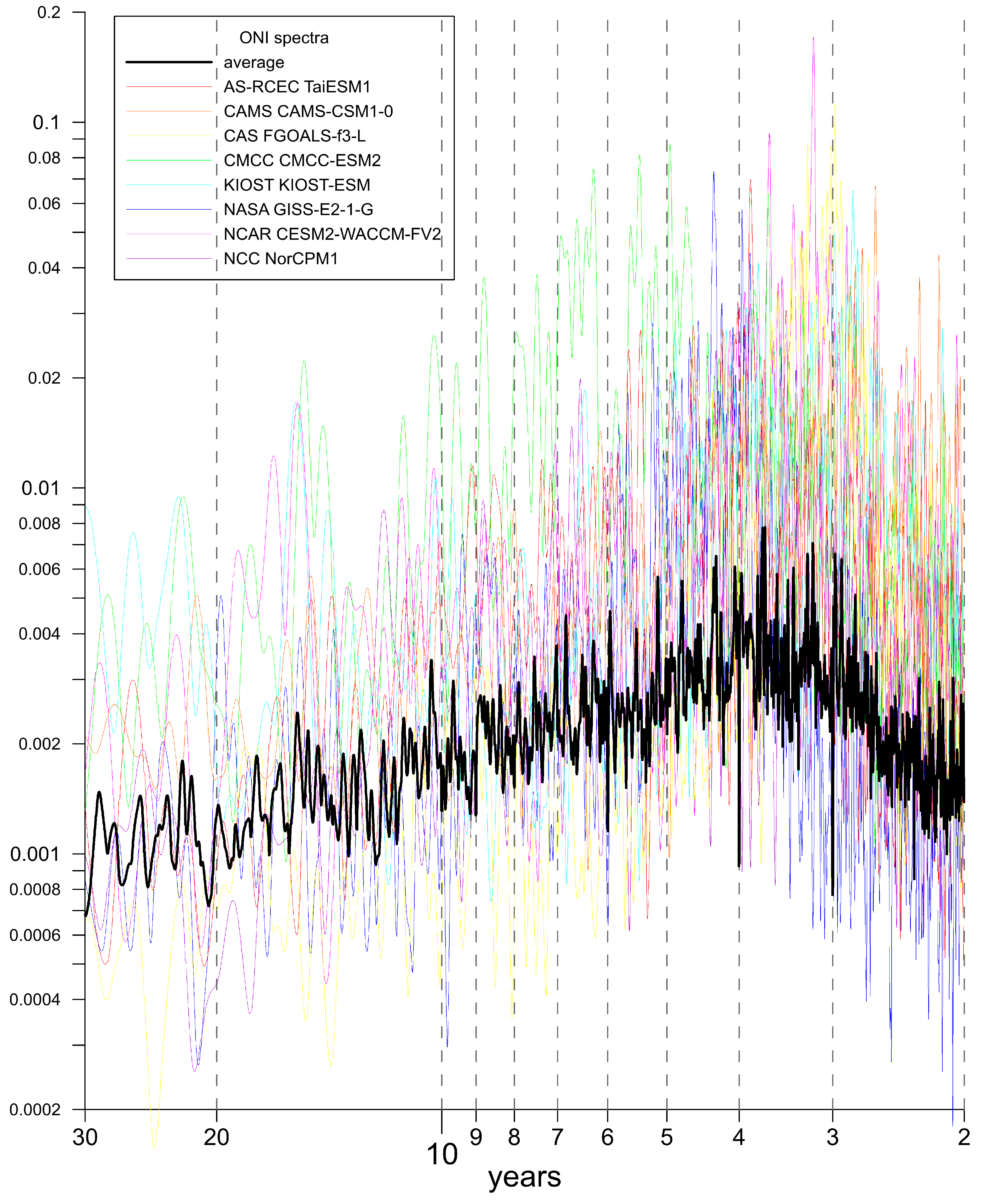
The ONI energy spectra of the eight selected CMIP6 models and the average spectrum for the considered 50 models (
Figure 5) differed from the SNA spectra. There were no obvious peaks in the average model’s ONI spectrum (
Figure 5, black line). In this case, an increase in the oscillation energy was observed from a period of 2 years to the maximum at periods of approximately 3.7–3.8 years. The oscillation energies then began to decrease from the maximum at periods of approximately 3.7–3.8 years until periods of approximately 30 years, after which the decrease slowed down. In this case, strong inter-model variability in the ONI spectra was observed.
The spectra of the ENSO and GAO indices obtained previously [
33] contained peaks at the periods of super- and sub-harmonics of the following external forces affecting the global climate system: the Chandler wobble of the Earth’s poles (period of ~1.2 years), changes in the solar activity (period of ~11.2 years), and the lunisolar nutation of the Earth’s rotation axis (period of ~18.6 years). There was no forcing of these external forces in the piControl experiment, and, therefore, no pronounced peaks with the indicated periods were observed in the average ONI spectrum of the CMIP6 models.
4. Conclusions
The 50 CMIP6 models considered had noticeable differences among themselves in the following ENSO characteristics: the standard deviation of the ONI, its minimum and maximum values, the average period of oscillation, and the average duration of El Niño and La Niña events. Some of the CMIP6 models reproduced these characteristics of the ONI and the asymmetry between El Niño and La Niña events, with the differences from those observed based on instrumental measurements. Therefore, we concluded that not all CMIP6 models satisfactorily reproduced the important characteristics of ENSO.
Despite this, many of the CMIP6 models reproduced well the global structure of the amplitude fields of the fluctuations in ST and SLP anomalies between El Niño and La Niña events, which were symmetrical relative to the equator, taking into account the location of the continents. Moreover, compared to the CMIP5 models, the number of CMIP6 models that reproduced the global structure of the amplitude of the ST and SLP anomaly oscillations between opposite phases of ENSO was higher. Thus, it was concluded that the CMIP6 models demonstrated an improved description of the teleconnections between ENSO and the studied meteorological fields outside the tropical Pacific Ocean compared to the CMIP5 models.
The average CMIP6 model fields of the ST and SLP anomaly oscillation amplitudes between the El Niño and La Niña events contained many of the same details as the fields of the GAO previously obtained from measurement data and reanalyses. At the same time, the inter-model variability in the amplitude of oscillations of these anomalies turned out to be comparable in some regions with their values, which indicates differences in the reproduction of ENSO teleconnections using the studied models. It was found that the AS-RCEC TaiESM1, CAMS CAMS-CSM1-0, CAS FGOALS-f3-L, CMCC CMCC-ESM2, KIOST KIOST-ESM, NASA GISS-E2-1-G, NCAR CESM2-WACCM-FV2, and NCC NorCPM1 models demonstrated high correlations between ENSO and SLP anomalies outside the tropics of the Pacific Ocean; for the other models, these values turned out to be lower.
The estimates of the energy spectra of the ONI obtained from the CMIP6 models differed from each other, as well as from the spectra obtained previously from observational data, where peaks were observed at periods of super- and sub-harmonics of external forces affecting the climate system. Thus, different temporal dynamics of ENSO were calculated among the CMIP6 models, and these dynamics also differed from those observed from the measurement data. The reason for this may be that, in the piControl experiment, with the exception of the annual cycle of heat input from the sun, there was no influence of other quasi-periodic external forces on the global climate system.


