Article

Quantifying the Atmospheric Water Balance Closure over Mainland China Using Ground-Based, Satellite, and Reanalysis Datasets

1
School of Electronic and Information Engineering, Beihang University, Beijing 100191, China
2
Meteorological Observation Centre of China Meteorological Administration, Beijing 100081, China
3
Research Institute for Frontier Science, Beihang University, Beijing 100191, China
*
Author to whom correspondence should be addressed.
Atmosphere 2024, 15(4), 497; https://doi.org/10.3390/atmos15040497
Submission received: 19 March 2024 / Revised: 5 April 2024 / Accepted: 10 April 2024 / Published: 18 April 2024

Abstract

:
Quantifying the atmospheric water balance is critical for the study of hydrological processes in significant regions. This study quantified atmospheric water balance closure at 205 stations in mainland China on a monthly timescale from 2009 to 2018 using datasets from ground- and satellite-based observations and reanalysis data. The closure performances were firstly quantified using the mean and root mean square (RMS) of the residuals, and the possible influencing factors were explored, as well as the influence of different water balance components (WBCs) using different datasets. In the closure experiment using ERA5, the mean and residuals were 6.26 and 12.39 mm/month, respectively, on average, which indicated a closure uncertainty of 12.8%. Using ERA5 analysis as a reference, the closure experiment using different combinations revealed average mean residuals of 8.73, 11.50, and 15.89 mm/month, indicating a precipitation closure uncertainty of 22.0, 23.7, and 24.4% for the ground- and satellite-based observations and reanalysis data, respectively. Two possible influencing factors, station latitude and the climatic zone in which the station is located, were shown to be related to closure performance. Finally, the analysis of the impact from different WBCs showed that precipitation tended to have the most significant impact, which may have been due to larger observation uncertainties. Generally, the atmospheric water balance in mainland China can be closed using datasets from different observational techniques.

1. Introduction

As one of the fundamental properties of planetary physical systems, atmospheric water balance is strongly coupled to global land–atmosphere hydrological circulation [1]. Thoroughly comprehending the atmospheric water balance helps to reveal the mechanisms associated with the hydrologic cycle and realize its management at regional and global scales [2,3].
Profiting from the rapid development of Earth observational technology, various platforms for monitoring water balance components (WBCs), including precipitation, evapotranspiration, atmospheric water vapor, and moisture divergence, have been established and are involved in water balance closure [4,5,6]. Currently, WBC monitoring based on ground- and satellite-based observations and models driven by other observations (reanalysis and land surface) are the most widely used methods for water cycle studies [7]. However, owing to the existence of heterogeneities, uncertainties, and systematic biases among the different techniques, the current observation of WBCs fails to guarantee a balance between them [8]. Previous studies have demonstrated that the current water balance from different observations is imbalanced at both terrestrial [9,10] and atmospheric scales [11,12]. Moreover, anthropogenic activity and global climate change have altered the global atmospheric water balance [13,14,15]. For these reasons, researchers in the climate community have been motivated to evaluate current state-of-the-art water balance closure using observations from different techniques over the past decades.
Numerous studies have evaluated atmospheric water balance closure using WBCs derived from various observational techniques. Reanalysis can provide worldwide and continuous information on WBC variability [16] and has been widely used to study water balance closure. For example, Trenberth et al. assessed the hydrological cycle balance using data from eight atmospheric reanalyses [17]. They found that the atmospheric water balance was not closed in most of the reanalyses, revealing significant differences compared with the observational estimates of the surface return flow. Lorenz and Kunstmann compared global closure performances using three reanalyses with independent observations [18]. They discovered that inconsistencies in precipitation minus evapotranspiration (P-E) over land and ocean caused an imbalance in the atmospheric water cycle, which resulted from the assimilation of unreliable satellite-based observations. Nowadays, new generations of reanalysis, such as MERRA-2 (Modern-Era Retrospective Analysis for Research and Applications) and ERA5 (fifth-generation of ECMWF (European Center for Medium-Range Weather Forecasts) reanalysis), have been improved in spatiotemporal resolution, input data record consistency, and assimilation model homogeneity. Evaluation of these datasets for the closure of water balances has shown that they generally exhibited improvements over their predecessors in balancing the water cycle [19,20].
Apart from reanalyses, satellite-based earth observations can also provide sufficient sources for WBC monitoring, and atmospheric water balance closure using satellite-based and reanalysis datasets has been conducted globally. Park et al. examined atmospheric water balance over the ocean using satellite-based and merged datasets [21]. The results showed that different combinations of datasets differed significantly in terms of residual intensities and distributions. Brown and Kummerow conducted a closure experiment in five tropical ocean regions using independent satellite-based observations and reanalysis data [22]. It showed that the Indian Ocean attained the highest performance with an imbalance of −3.0%, whereas the western Pacific Ocean displayed the lowest performance with an imbalance of −21.1%. Eyre and Zeng assessed the capability of combining remote sensing and reanalysis datasets for characterizing the water cycle in the Amazon region [23]. They demonstrated that the Amazon Basin water balance could be closed with specific dataset combinations, whereas using other ensemble datasets resulted in a large mean residual.
It is noteworthy that assessing regional water balance closure may help improve global water cycle estimation [24]. Although previous studies have contributed greatly to closing the atmospheric water balance globally and in specific locations, closure characteristics in hydrologically significant regions, such as China, have rarely been discussed. China is located in East Asia and is adjacent to the western Pacific Ocean, where it is influenced by complex Asian monsoon systems [25,26]. It has a vast territory and a three-step staircase with an eastward descending topography, resulting in diverse climatic conditions and complex hydrological characteristics [27]. Due to its distinct location, China’s atmospheric water balance has a conspicuous impact on its surrounding areas in the Asia–Pacific region. Therefore, a comprehensive atmospheric water balance analysis in mainland China is of vital importance.
This study aimed to quantify the atmospheric water balance closure at 205 stations in mainland China at a monthly temporal resolution from 2009 to 2018. Datasets derived from ground- and satellite-based observations and reanalysis data were used to obtain the WBCs for analysis. The closure performance using WBC combinations from different datasets was examined and discussed, which will be helpful for hydrological cycle studies in mainland China. The remainder of this paper is organized as follows: Section 2 describes the datasets and quantification methods, including data processing strategies. Section 3 presents the analysis and discussion of the closure experiment results, and conclusions are drawn in Section 4.

2. Methodology

This section describes the methods used for the experiments, including the data description, an approach for quantifying atmospheric water balance closure, a method for deriving WBCs from gridded-based datasets, and a height correction procedure for GPS-derived water vapor. A general flow chart of this experiment is presented in Figure 1, as follows.

2.1. Description of the Datasets

Multiple datasets from various observational techniques were used to obtain the WBCs from 2009 to 2018, including ground- and satellite-based observations, and reanalysis data, as summarized in Table 1. Comprehensive descriptions of the datasets are provided below.

2.1.1. Ground-Based Observational Datasets

Ground-based observations of precipitation and evapotranspiration were obtained from 205 meteorological stations established by the China Meteorological Administration (CMA) in mainland China. Integrated daily observational records were adopted and calculated using monthly resolution for further analysis. The absent value owing to poor quality was interpolated using Deng et al.’s method [28] on a monthly timescale.
Note that only a few meteorological stations are equipped with radiosondes or microwave radiometers. Thus, ground-based water vapor was derived from a global positioning system (GPS) at an adjacent global navigation satellite system (GNSS) subordinated to the Crustal Movement Observation Network of China (CMONOC) maintained by the China Meteorological Administration (CEA) [29]. Detailed descriptions of monthly water vapor retrieval from raw GPS observations can be found in Zhou et al. [30]. The distribution of meteorological stations (hereafter called stations for convenience) is shown in Figure 2 to represent ground-based observational positions.

2.1.2. Satellite-Based Observational Datasets

Multiple satellite-based precipitation data were derived from the Global Precipitation Measurement (GPM) product because of its higher accuracy compared with other satellite-based precipitation products [31]. It can provide accurate global observations of rainfall from 2000 to the present. In this study, monthly satellite-based precipitation data were derived from the GPM IMERG final precipitation L3 V06 (GPM_3IMERGM) with a spatial resolution of 0.1 °   × 0.1 ° .
Evapotranspiration data were derived from the commonly used Moderate Resolution Imaging Spectroradiometer (MODIS) global evapotranspiration products, provided by National Aeronautics and Space Administration (NASA) Level-1 Atmosphere Archive and Distribution System Distributed Active Archive Center (LAADS DAAC) [32]. In this study, the MOD16 A2 product was selected to provide satellite-based evapotranspiration data with a spatial resolution of 0.5 °   × 0.5 ° , latitude of 80–60 ° N, and longitude of 0–360 ° E.
Water vapor data were derived from Atmospheric Infrared Sounder (AIRS) products, provided by NASA’s Goddard Earth Sciences Data and Information Services Center (GES DISC) [33]. Previous studies have demonstrated their superior performance over other products in mainland China [34]. In this study, the AIRS Level 3 daily gridded product (Version 7) was adopted, which provides daily averaged water vapor values on a global scale with a spatial resolution of 1 ° . Note that the daily observations of the AIRS should be calculated with a monthly temporal resolution before the following closure experiments.

2.1.3. Reanalysis Datasets

Latest-generation reanalysis datasets, ERA5 and MERRA-2, were selected due to their better performance over those of their predecessors [35,36]. ERA5 covers the period from 1979 to the present and has a spatial resolution of 0.25 °   × 0.25 ° at the global scale. MERRA-2 covers the period from 1980 to the present and has a spatial resolution of 0.5 ° latitude × 0.625 ° longitude at the global scale. Both reanalysis products provide precipitation, evapotranspiration, and water vapor data, whereas ERA5 provides moisture divergence data directly without additional calculations. ERA5 provides a better representation of long-term wind variability than MERRA-2 [37], which significantly influences the accuracy of moisture divergence. Therefore, in this study, moisture divergence was derived only from the ERA5 product.

2.2. Quantification of Atmospheric Water Balance Closure in Mainland China

The atmospheric water balance can be generally described as follows [38]:
· Q + d W d t ( E P ) = 0
where E and P represent evapotranspiration and precipitation, respectively. Q is the vertically integrated water vapor flux, whereas ∇∙Q indicates its divergence (denoted as Div). W indicates the total column water vapor from the surface to the top of the atmosphere (TOA), whereas dW/dt represents its change between two months (denoted as ∆W, water vapor change), which was calculated using the forward differences:
W i = ( d W d t ) i = W i + 1 W i
To avoid introducing any artificial lag due to the difference procedure [39], other WBCs in Equation (1) ( P , E , and ∇∙Q, denoted as X in the following equation) needed to be time-filtered as follows:
X ~ i = X i + 1 + X i 2
To quantify the closure performance, the residual of Equation (1) was calculated as follows:
R e s = E P · Q d W d t
where R e s represents the atmospheric water balance residual obtained from different WBC combinations. Two evaluation metrics were adopted to examine the closure performance: the mean and root mean square (RMS) of the residual. A positive value of the residual mean indicates that the magnitudes of the atmospheric water vapor source terms (evapotranspiration and moisture divergence) are greater than those of the sink terms (precipitation and water vapor change), whereas a negative value indicates the opposite.
Moreover, to analyze the influence of different WBCs and observational techniques on closure performance, the control variate technique was adopted to examine the performance differences using WBCs (precipitation, evapotranspiration, and water vapor change) from different datasets.

2.3. WBC Derivation from Gridded-Based Datasets

For consistency with ground-based observations, WBCs from gridded-based datasets, including satellite-based observations and reanalysis, should be derived at a specific station location. To optimally mitigate the additional error induced by the interpolation procedure, the nearest-neighbor method was directly applied to obtain WBCs from gridded-based products at a specific spatial location to avoid the influence of spatial resampling.
Moreover, the GPS-derived water vapor represents the integrated value from the height of the antenna to the TOA, whereas the gridded-based water vapor represents the mean value within a specific grid. However, the mean grid point and station elevations are not generally consistent [40], which causes a bias because water vapor exponentially decreases with an increase in height [41]. Hence, a height correction procedure is conducted to modify the GPS-derived water vapor (denoted as precipitable water (PW)) from the height of the station antenna to the surface height according to Kouba [42], as calculated in the following equation:
P W m o d = P W o r i · e x p ( H 1 H 0 2000 )
where PWori and H0 represent the original water vapor value and height of the station antenna, respectively, and PWmod and H1 represent the modified water vapor value and surface grid height, respectively. The station surface heights were derived from the Terra Advanced Spaceborne Thermal Emission and Reflection Radiometer Global Digital Elevation Model Version 3.

3. Results and Discussion

This section presents the quantification of atmospheric water balance closures in mainland China using WBC combinations of datasets from different observation techniques. First, closure performance was evaluated using combinations of different observation techniques. Subsequently, the possible factors influencing closure performance were analyzed. Finally, the influence of different WBCs and observation techniques on the closure performance was assessed using the control variate technique.

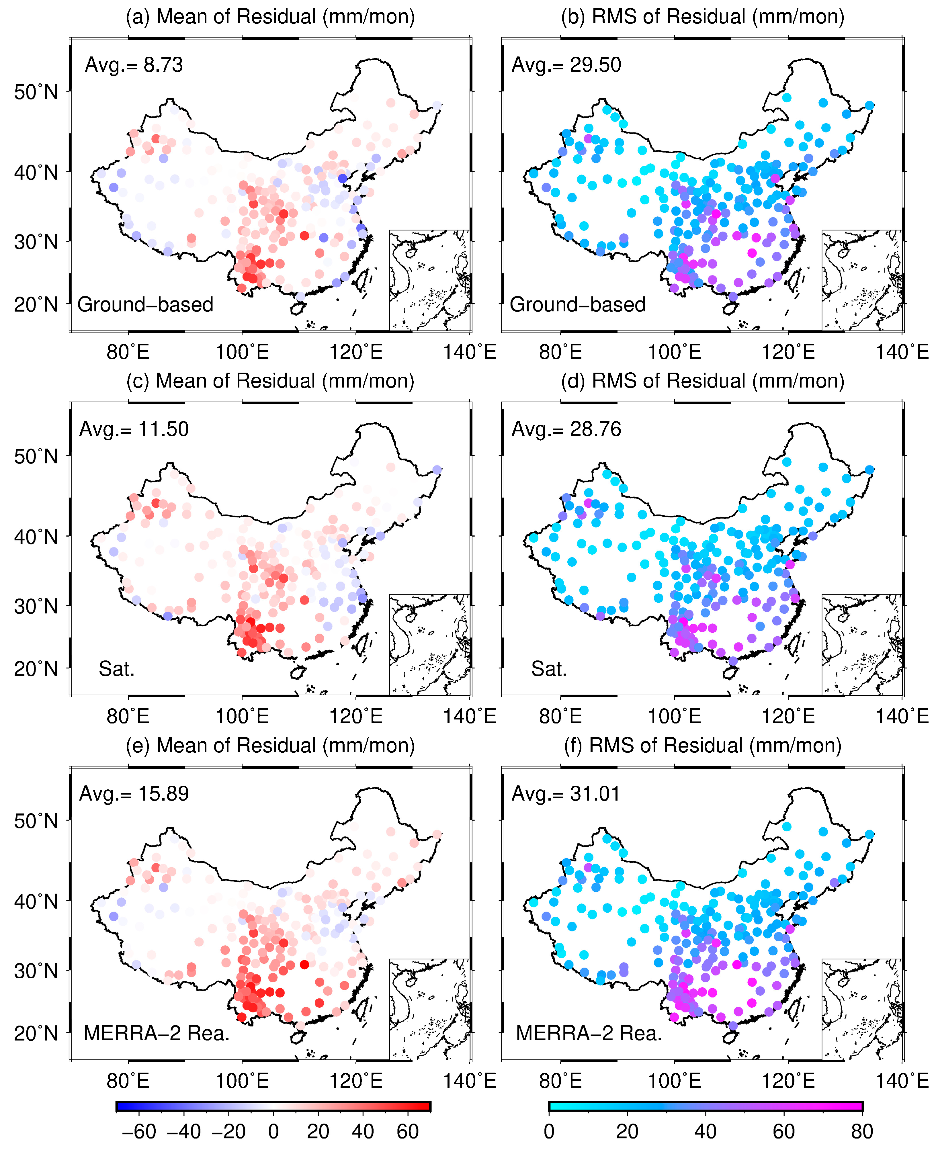
3.1. Quantifying the Performances of Atmospheric Water Balance Closure Using WBC Combinations from Different Observation Techniques

The atmospheric water balance closure performance using WBCs from ground- and satellite-based observations, and reanalysis data, was evaluated and discussed. The WBC combinations from different observation techniques are listed in Table 2. The closure performance using the WBCs from ERA5 was first assessed using the mean and RMS of the atmospheric water balance residuals for all stations, as shown in Figure 3. The results showed that the average mean and RMS of the residuals were 6.26 and 12.39 mm/month for all stations, respectively. Rodell et al. indicated that closure uncertainty can be presented as a percentage of annual precipitation [43]. Thus, the ERA5 results revealed an average closure uncertainty of 12.8% in precipitation at all stations in mainland China. This was acceptable at monthly timescales for continental regions [44]. This demonstrates that despite the fact that the atmospheric water balance was not constrained in the ERA5 generation [7], it still exhibited good performance for atmospheric water balance closure.
Further analysis of the spatial distribution of the mean residual showed that most stations in mainland China exhibited positive values, except for some stations located at the edges of the Tibetan Plateau (TP). This indicates that the atmospheric water vapor source terms are generally higher than the sink terms for mainland China. This is because (1) China is located in the low- and mid-latitude zones, where sufficient sunshine induces sufficient evapotranspiration from land to the atmosphere [45,46], and (2) China is located in East Asia and is adjacent to the Pacific, where the monsoons transport sufficient water vapor from the oceans to mainland China [47,48]. These two factors contribute to the higher source terms of atmospheric water vapor, which lead to positive values for the mean residual for most stations in mainland China. For the RMS residual, stations within China’s southern and eastern regions generally showed higher RMS values, whereas other regions, particularly the TP, showed relatively lower RMS values. These results indicate that the closure performance of ERA5 differs among different regions within mainland China. Some stations in the northwestern region of China showed a high RMS residual. This is because these stations are located on the northern slope of the Tianshan Mountain and at the boundary of climatic zones where the topography and atmospheric circulation characteristics are complex [49,50]. The accuracy of ERA5 may be inferior in such regions. In general, the WBCs derived from ERA5 exhibited good performance in atmospheric water balance closure in mainland China. Thus, it can serve as a reference for examining the closure performance using WBC combinations from various observation techniques.
Subsequently, the atmospheric water balance closure performance using WBCs from three combinations of observation techniques, ground- and satellite-based observations, and reanalysis data, was evaluated in mainland China. The spatial distributions of the mean and RMS residuals for all stations from the three combinations are presented in Figure 4. Note that the scaling in Figure 4 differs from that in Figure 3.
Generally, the closure performances using WBCs from the three combinations of observational techniques were inferior to those obtained from ERA5. The statistical results showed that the atmospheric water balance closure using combinations of ground-based observed, satellite, and reanalysis data revealed average mean residuals of 8.73, 11.50, and 15.89 mm/month, respectively. These values indicate that the closure uncertainties were 22.0, 23.7, and 24.4% of precipitation for different observation techniques, respectively. Rodell et al. indicated that the atmospheric water balance can be closed with an uncertainty of approximately 20% of precipitation on a monthly timescale for continental regions [43]. This indicates that, despite being inferior to datasets using WBCs from ERA5, the atmospheric water balance can be closed using datasets from different observational techniques in mainland China. Among the three combinations of observational techniques, ground-based observations attained the lowest average mean residuals. This might indicate that the actual observation of WBCs generally had the lowest systematic bias. In contrast to the mean residuals, the corresponding RMS residuals for the three combinations attained averages of 29.50, 28.76, and 31.01 mm/month, respectively. This indicates that different combinations generally exhibit similar closure performance in mainland China. Note that the reanalysis combination using WBC data from MERRA-2 performed slightly inferior to those of ground- and satellite-based observations, with the highest mean and RMS residuals. This may be because the spatial resolution of MERRA-2 was lower than that of the other grid datasets (except for AIRS), which made it more difficult to characterize the actual values of WBCs, especially precipitation, for each station.
Furthermore, the mean and RMS residual spatial distributions for all stations from different combinations were analyzed. Generally, it was observed that the evaluation metrics among different combinations shared similar spatial distributions in mainland China (Figure 3 and Figure 4). Nevertheless, different characteristics can still be recognized in the spatial distribution of the mean residuals. Some stations within the eastern region of China exhibited a negative mean residual for ground- and satellite-based observations (Figure 4a,c). However, these stations generally exhibited a positive mean residual using the WBCs from the reanalysis data (MERRA-2) (Figure 4e), which was consistent with the results obtained using ERA5 (Figure 3a). This might be because these stations are generally located in the East China (EC) and subtropical monsoon (SM) climatic zones, where the climate and hydrological cycles are complicated and susceptible to the influence of extreme weather events, such as tropical cyclones [51]. Considering that precipitation-related extreme events are more difficult to accurately capture using reanalysis datasets [52,53], the accuracy of the reanalysis data within these regions was generally inferior to that of ground-based data or satellite-based observations. In general, despite regional differences, the atmospheric water balance can be closed using WBCs from ground- and satellite-based observations and reanalysis datasets from mainland China. However, this method only considered the mass balance of the atmospheric water cycle; simultaneously considering the mass and the energy cycles should lead to a better understanding. Thus, a more systematical analysis both evaluating the mass and energy balance should be considered.

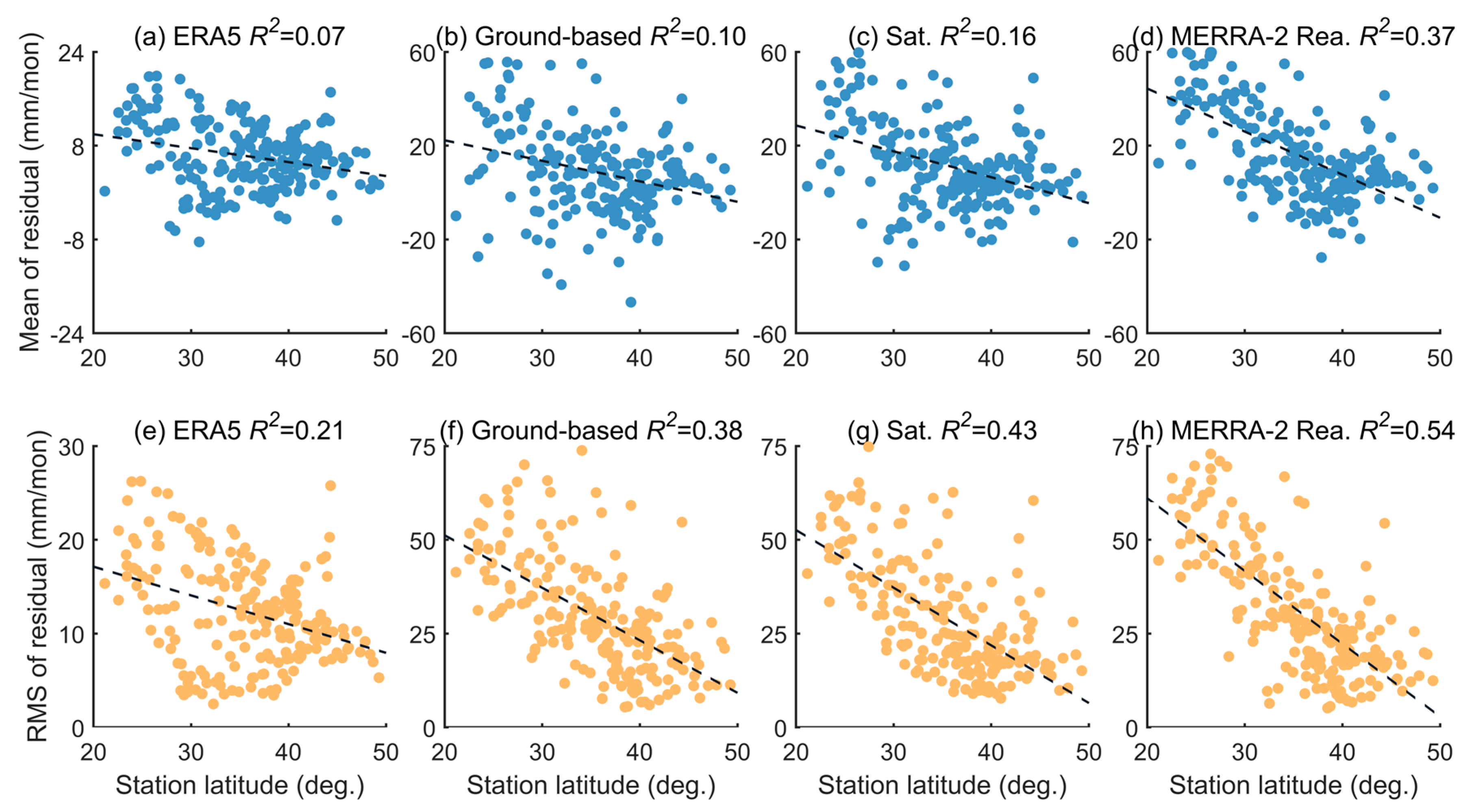
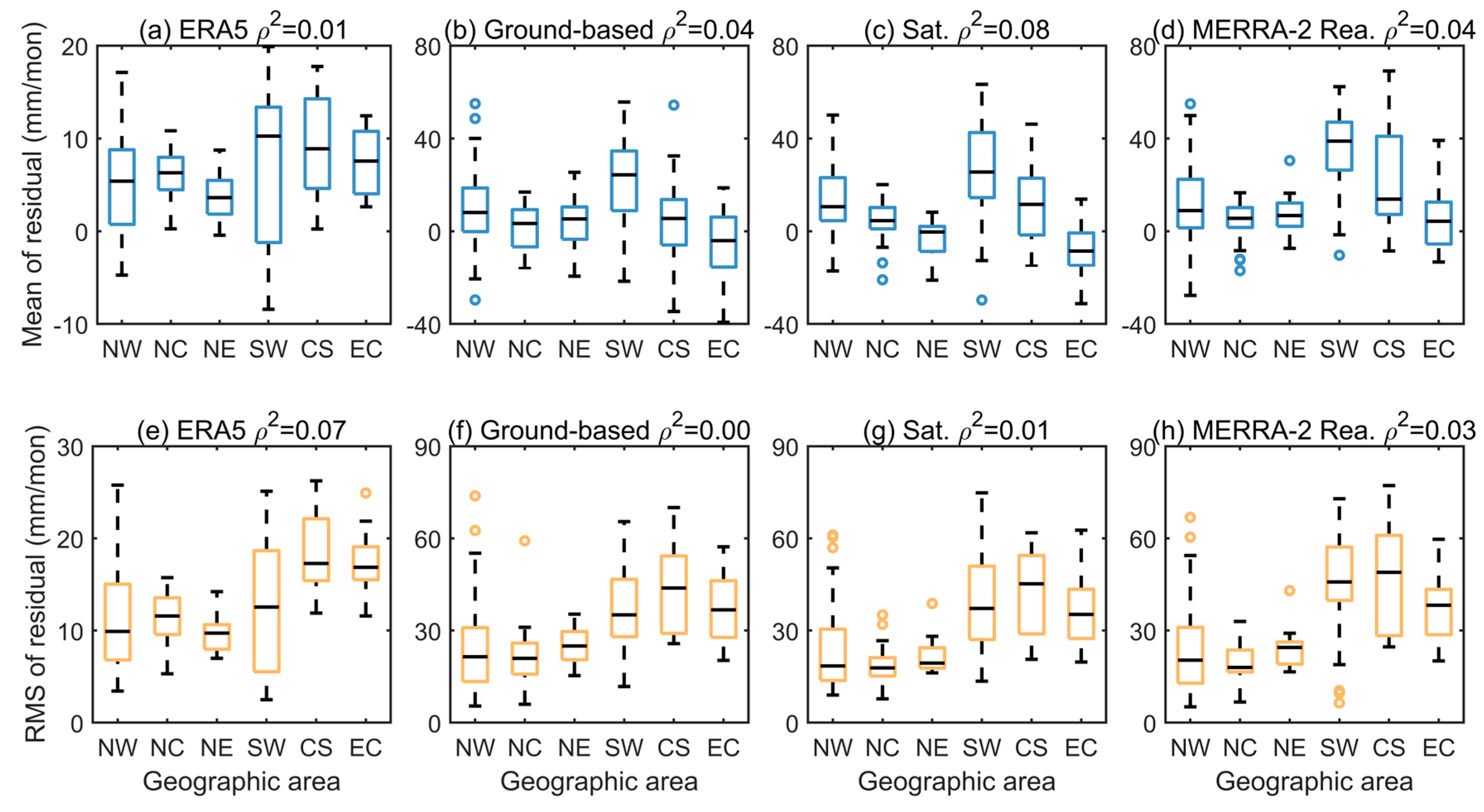
3.2. Analyzing the Possible Influencing Factors for Atmospheric Water Balance Closure Performance Using WBCs from Different Observation Techniques

To further explore the possible factors influencing closure performance in mainland China, the relationships among the evaluation metrics, geographic characteristics, and location types were analyzed. The geographic characteristics (represented by station height and latitude) are shown against the mean and RMS residuals in Figure 5 and Figure 6, respectively. The coefficient of determination (R2) was calculated to verify the relationship with 5% statistical significance tested using the t-test.
Regarding station height (Figure 5), only the mean and RMS residuals from the ERA5 combination showed negative relationships (R2 = 0.22 and 0.35, respectively), whereas this phenomenon was not observed in other combinations. This might be because the ERA5 dataset can capture the differences and variations in the atmosphere in the vertical direction more precisely than MERRA-2 [54] and other single-level observation techniques. The results of ERA5 coincide with Figure 3b in that higher mean and RMS values tend to appear for stations in the eastern region than those in the western region.
Regarding station latitude (Figure 5), the combinations of ground-based, satellite, and MERRA-2 reanalysis exhibited a negative relationship with the RMS residuals (R2 = 0.38, 0.43, 0.54, respectively), while this phenomenon was less apparent for ERA5 reanalysis (R2 = 0.21). This indicates that, despite the observational techniques, all dataset combinations generally attained better closure performances for stations at higher latitudes in mainland China. This phenomenon coincided with Figure 3 and Figure 4, which show that compared with the northern region of China, the RMS residual values for stations located in the southern region of China were generally higher. For the mean residuals, only MERRA-2 reanalysis datasets showed a possible correlation (R2 = 0.37). This indicated that atmospheric closure using WBCs from ERA5 and ground- and satellite-based observations was generally consistent among different latitudes, whereas inter-latitudinal consistency was not apparent for MERRA-2.
Subsequently, the location types (represented by geographic area and climatic zone) were analyzed, as shown in Figure 7 and Figure 8, respectively. Geographically, all stations were divided into Central South (CS), North China (NC), EC, North East (NE), North West (NW), and South West (SW) China. This division was based on criteria from the Institute of Geographic Sciences and Natural Resources Research, Chinese Academy of Sciences, which can be retrieved from https://www.resdc.cn/data.aspx?DATAID=276 (accessed on 24 January 2024). All stations were divided into plateau (PL), tropical monsoon (TM), humid continental (HC), mid-latitude monsoon (MM), and SM climatic zones according to the CMA criteria [55]. Note that the quantified relationships for the location types were calculated using squared Spearman’s rank correlation coefficient (denoted as ρ2). The significance test was conducted using Fisher transformation.
No obvious relationship was observed between closure performance and geographical area. Nevertheless, regional statistical results showed that the RMS residual values for the northern regions of mainland China (NW, NC, and NE) were lower than those for the southern regions of China (SW, CS, and EC). This phenomenon is consistent with the results presented in Section 3.1. However, statistically possible correlation relationships between the RMS residuals and climatic zones were observed for all combinations (ρ2 > 0.3). This may confirm that, despite the observational techniques, the closure performance of all combinations may have a distinct relationship with climatic conditions. The PL and HC climatic zones attained the best performances, whereas inferior performances were observed at stations within the SM and MM climatic zones. This may be due to the fact that compared with the PL or HC climatic zones, the SM and MM climatic zones were involved in complex coupled atmosphere–ocean–land processes [56,57]. This may introduce more observed uncertainties and unmodeled systematic errors for ground- and satellite-based observations, or reanalysis datasets in the SM and MM climatic zones. Generally, station latitude and the climate zone in which the station is located might have some impact on the closure performance. However, these results are not significant for all combinations; thus, a more comprehensive analysis should be conducted in the future to explore the mechanism for the influencing factors.

3.3. Analyzing the Influence of Different WBCs and Observational Techniques on Closure Performance through the Control Variate Technique

The influence of different WBCs and observational techniques on closure performance was analyzed using the control variate technique. The results of the closure experiments were compared with the closure performance obtained using WBCs from ERA5. The combinations of different datasets used for the closure experiments are listed in Table 3. The mean and RMS residuals from different combinations are presented in Figure 9. The Pauta criterion (3-sigma criterion) was employed to eliminate stations with gross errors, and no more than four stations were eliminated for each combination.
The influence of different WBCs on closure performance was first analyzed by comparing the average values of the evaluation metrics using different datasets of a specific WBC with the ERA5 results as a reference. The greatest discrepancy between the evaluation metrics was observed when different precipitation datasets were used. The difference between the average mean and RMS residuals using three different precipitation datasets and ERA5 was 7.72 and 16.86 mm/month, respectively. The smallest discrepancy between the evaluation metrics was observed when different water vapor datasets were used. The difference between the average mean and RMS residuals using three different water vapor datasets and ERA5 was −0.01 and 0.84 mm/month, respectively. This phenomenon may be due to different observational uncertainties for different WBCs. For precipitation, relatively large observational uncertainties are introduced owing to different assumptions, techniques, and calibration methods [58]. Even for the most accurate rain gauge measurements [59,60], wind effects cause systematic measurement errors [7]. These uncertainties significantly influence water balance closure [61].
Subsequently, the influence of datasets from different observational techniques on closure performance was discussed for each WBC. For precipitation, three different datasets exhibited mean residual values of 11.51, 13.86, and 16.58 mm/month, respectively, whereas the corresponding RMS residual values were 29.43, 28.82, and 29.51 mm/month, respectively. These values are higher than those obtained using ERA5, which may be due to the differences between these three precipitation datasets and ERA5. Among the different datasets, although RMS residual values were generally close to each other, the ground-based observations attained the lowest mean residuals. This indicates that ground-based precipitation observations attained the lowest observable uncertainties.
For evapotranspiration, the mean residual values were 3.85, 3.93, and 5.65 mm/month for three different datasets, respectively. The corresponding RMS residual values were 17.96, 17.01, and 19.05 mm/month, respectively. In contrast to precipitation, the mean residual values using ground- and satellite-based observations were lower than those using ERA5, whereas those of the MERRA-2 reanalysis data were higher than those of ERA5. This may be because evapotranspiration values obtained from ground- and satellite-based observations are more accurate and have lower uncertainties than those obtained from model-derived datasets (the land surface model and reanalysis) [62,63], although these have been greatly improved in comparison to their predecessors [64].
For water vapor change, the results exhibited mean residual values of 6.24, 6.25, and 6.24 mm/month for three different datasets, respectively. The corresponding RMS residuals were 13.17, 12.92, and 13.61 mm/month, respectively. These values were comparable to those of ERA5, indicating that different sources of water vapor had little impact on the performance of atmospheric water vapor closure. As stated above, the magnitude of water vapor change was much smaller than that of the other WBCs in the atmospheric water balance equation. Thus, the observable uncertainties introduced by water vapor from different datasets did not significantly influence closure performance.
Subsequently, the average time series of the residuals and their anomalies estimated using the abovementioned WBC combinations were analyzed and are shown in Figure 10. Distinct annual variations were observed for all combinations, which is consistent with previous studies. In Park et al. (2013), discernable annual variation was observed in the time series of nine monthly domain-averaged residuals using satellite-based and merged datasets for the atmospheric water cycle [21]. This residual was relatively larger in summer than in winter. However, this phenomenon was not discussed. For our study, we thought that this indicates that some unmodeled errors in the annual period occur in atmospheric closure. We considered that this may be partly due to the neglected time rate of the change in liquid and solid water in clouds (∆W). Despite the slight impact due to the numerical magnitude of ∆W, the accumulated effects from cloud liquid and ice still require further investigation and analysis to improve closure performance. Moreover, a distinctly negative trend was observed for all combination residuals, indicating that the closure means that the residuals gradually approached zero over time. This may be because the current availability of sufficient observations and accurate models means that observable uncertainties and systematic biases are much smaller than before, thus improving closure performance. In addition, the amplitudes of the residuals were reduced, except for those of ERA5. This may be because ERA5 used a consistent model for different times, and the character of the residual was also consistent at different times.

4. Conclusions

Quantifying atmospheric water balance closure is vital for understanding the hydrological cycle. In this study, the atmospheric water balance closure from 2009 to 2018 was evaluated using WBCs from different observational techniques. Generally, the atmospheric water balance in mainland China can be closed using WBCs from different observational techniques. The ERA5 results showed that the average RMS residuals were 12.39 mm/month, revealing a precipitation closure uncertainty of 12.8%. The closure performance using WBC combinations from ground- and satellite-based observations and MERRA-2 reanalysis showed average residual values of 8.73, 11.50, and 15.89 mm/month, respectively. These values indicate closure uncertainties of 22.0, 23.7, and 24.4% for precipitation.
Subsequently, the relationships between the evaluation metrics and possible influencing factors were analyzed. The results indicated that station latitude and the climatic zone in which a station is located showed some possible correlating relationship with closure performance. However, a more comprehensive analysis ought to be carried out to further explore the inherent mechanism.
Finally, the closure performances of WBCs from different datasets were compared using the control variate technique. The results showed that precipitation represented the largest contribution to closure performance, whereas water vapor change contributed the least. This is attributable to the relatively large observational uncertainty of precipitation. Moreover, the average closure residuals gradually approached zero, with a negative trend for the residuals of all combinations owing to additional observations and accurate models.
Future research lies in two directions. First, a more comprehensive analysis should be conducted to further explore the effects and mechanisms of climatic conditions on closure performance. Second, considering that the mass and energy balance simultaneously leads to a better understanding of the water cycle, a more systematical experiment should be carried out to explore the coupled relationship between mass and energy balance.

Author Contributions

Conceptualization, L.Z., Y.C. and H.L.; methodology, L.Z.; software, L.Z. and L.F.; validation, L.Z. and Y.C.; formal analysis, L.Z., Y.C. and H.L.; investigation, L.Z., Y.C. and H.L.; resources, L.Z., H.L., L.F. and C.S.; writing—original draft preparation, L.Z.; writing—review and editing, L.Z., Y.C., L.F. and H.L.; visualization, L.Z.; supervision, L.F., Y.C. and C.S.; funding acquisition, L.F. and C.S. All authors have read and agreed to the published version of the manuscript.

Funding

This work was sponsored by the National Natural Science Foundation of China (Grant No. 41931075, 41961144015) and Observational Experiment Project of Meteorological Observation Center of China Meteorological Administration (Grant No. GCSYJH23-04).

Institutional Review Board Statement

Not applicable.

Informed Consent Statement

Not applicable.

Data Availability Statement

The authors are grateful to the CMA for providing ground-based observation data, the CEA for providing GPS observations at adjacent GNSS stations, NASA for providing the AIRS, MODIS, GPM, and MERRA-2 data, and ECMWF for providing the ERA5 data. The ground-based observations of the meteorological stations are available from the CMA at http://data.cma.cn/ (accessed on 11 April 2024). The GPM IMERG Final Precipitation L3 V06 is available from the GES DISC at https://disc.gsfc.nasa.gov/datasets/GPM_3IMERGM_06/summary?keywords=GPM (accessed on 11 April 2024). The MOD16 A2 is available from the https://ladsweb.modaps.eosdis.nasa.gov/missions-and-measurements/products/MOD16A2 (accessed on 11 April 2024). The AIRS Level 3 Daily Gridded Product (Version 7) is available from the LAADS DAAC at https://ladsweb.modaps.eosdis.nasa.gov/missions-and-measurements/products/MOD16A2 (accessed on 11 April 2024). The MERRA-2 is available from the GES DISC at https://disc.gsfc.nasa.gov/datasets?keywords=MERRA2&page=1 (accessed on 11 April 2024). The ERA5 monthly averaged data on single levels data are available from the CDS at https://cds.climate.copernicus.eu/cdsapp#!/dataset/reanalysis-era5-single-levels-monthly means?tab=overview (accessed on 11 April 2024). The ASTGTM data are available from the LP DAAC at https://lpdaac.usgs.gov/products/astgtmv003/ (accessed on 11 April 2024). The criterium for the division of geographical areas is available from the Resource and Environment Science and Data Center, Institute of Geographic Sciences and Natural Resources Research, Chinese Academy of Sciences at https://www.resdc.cn/data.aspx?DATAID=276 (accessed on 11 April 2024). The GPS observations can be accessed only with an official application to the China Earthquake Administration due to a confidentiality agreement.

Conflicts of Interest

The authors declare no conflict of interest.

References

  1. Dagan, G.; Stier, P.; Dingley, B.; Williams, A.I. Examining the regional co-variability of the atmospheric water and energy imbalances in different model configurations-linking clouds and circulation. J. Adv. Model. Earth Syst. 2022, 14, e2021MS002951. [Google Scholar] [CrossRef] [PubMed]
  2. Yarosh, E.S.; Ropelewski, C.F.; Berbery, E.H. Biases of the observed atmospheric water budgets over the central United States. J. Geophys. Res. Atmos. 1999, 104, 19349–19360. [Google Scholar] [CrossRef]
  3. Wang, S.; Huang, J.; Li, J.; Rivera, A.; McKenney, D.W.; Sheffield, J. Assessment of water budget for sixteen large drainage basins in Canada. J. Hydrol. 2014, 512, 1–15. [Google Scholar] [CrossRef]
  4. Liepert, B.G.; Previdi, M. Inter-model variability and biases of the global water cycle in CMIP3 coupled climate models. Environ. Res. Lett. 2012, 7, 014006. [Google Scholar] [CrossRef]
  5. Luo, Z.; Shao, Q.; Wan, W.; Li, H.; Chen, X.; Zhu, S.; Ding, X. A new method for assessing satellite-based hydrological data products using water budget closure. J. Hydrol. 2021, 594, 125927. [Google Scholar] [CrossRef]
  6. Su, Y.; Smith, J.A. An atmospheric water balance perspective on extreme rainfall potential for the contiguous US. Water Resour. Res. 2021, 57, e2020WR028387. [Google Scholar] [CrossRef]
  7. Dorigo, W.; Dietrich, S.; Aires, F.; Brocca, L.; Carter, S.; Cretaux, J.F.; Dunkerley, D.; Enomoto, H.; Forsberg, R.; Güntner, A.; et al. Closing the water cycle from observations across scales: Where do we stand? Bull. Am. Meteorol. Soc. 2021, 102, E1897–E1935. [Google Scholar] [CrossRef]
  8. Albergel, C.; Dorigo, W.; Reichle, R.H.; Balsamo, G.; De Rosnay, P.; Muñoz-Sabater, J.; Isaksen, L.; De Jeu, R.; Wagner, W. Skill and global trend analysis of soil moisture from reanalyses and microwave remote sensing. J. Hydrometeorol. 2013, 14, 1259–1277. [Google Scholar] [CrossRef]
  9. Sheffield, J.; Ferguson, C.R.; Troy, T.J.; Wood, E.F.; McCabe, M.F. Closing the terrestrial water budget from satellite remote sensing. Geophys. Res. Lett. 2009, 36, L07403. [Google Scholar] [CrossRef]
  10. Abolafia-Rosenzweig, R.; Pan, M.; Zeng, J.L.; Livneh, B. Remotely sensed ensembles of the terrestrial water budget over major global river basins: An assessment of three closure techniques. Remote Sens. Environ. 2021, 252, 112191. [Google Scholar] [CrossRef]
  11. Yu, L.; Jin, X.; Josey, S.A.; Lee, T.; Kumar, A.; Wen, C.; Xue, Y. The global ocean water cycle in atmospheric reanalysis, satellite, and ocean salinity. J. Clim. 2017, 30, 3829–3852. [Google Scholar] [CrossRef]
  12. Builes-Jaramillo, A.; Poveda, G. Conjoint analysis of surface and atmospheric water balances in the Andes-Amazon system. Water Resour. Res. 2018, 54, 3472–3489. [Google Scholar] [CrossRef]
  13. Schlosser, C.A.; Houser, P.R. Assessing a satellite-era perspective of the global water cycle. J. Clim. 2007, 20, 1316–1338. [Google Scholar] [CrossRef]
  14. Abdulla, F.; Eshtawi, T.; Assaf, H. Assessment of the impact of potential climate change on the water balance of a semi-arid watershed. Water Resour. Manag. 2009, 23, 2051–2068. [Google Scholar] [CrossRef]
  15. Abbott, B.W.; Bishop, K.; Zarnetske, J.P.; Minaudo, C.; Chapin, F.S., III; Krause, S.; Hannah, D.M.; Conner, L.; Ellison, D.; Godsey, S.E.; et al. Human domination of the global water cycle absent from depictions and perceptions. Nat. Geosci. 2019, 12, 533–540. [Google Scholar] [CrossRef]
  16. Auerbach, D.A.; Easton, Z.M.; Walter, M.T.; Flecker, A.S.; Fuka, D.R. Evaluating weather observations and the Climate Forecast System Reanalysis as inputs for hydrologic modelling in the tropics. Hydrol. Process. 2016, 30, 3466–3477. [Google Scholar] [CrossRef]
  17. Trenberth, K.E.; Fasullo, J.T.; Mackaro, J. Atmospheric moisture transports from ocean to land and global energy flows in reanalyses. J. Clim. 2011, 24, 4907–4924. [Google Scholar] [CrossRef]
  18. Lorenz, C.; Kunstmann, H. The hydrological cycle in three state-of-the-art reanalyses: Intercomparison and performance analysis. J. Hydrometeorol. 2012, 13, 1397–1420. [Google Scholar] [CrossRef]
  19. Bosilovich, M.G.; Robertson, F.R.; Takacs, L.; Molod, A.; Mocko, D. Atmospheric water balance and variability in the MERRA-2 reanalysis. J. Clim. 2017, 30, 1177–1196. [Google Scholar] [CrossRef]
  20. Mayer, J.; Mayer, M.; Haimberger, L. Consistency and homogeneity of atmospheric energy, moisture, and mass budgets in ERA5. J. Clim. 2021, 34, 3955–3974. [Google Scholar] [CrossRef]
  21. Park, H.J.; Shin, D.B.; Yoo, J.M. Atmospheric water balance over oceanic regions as estimated from satellite, merged, and reanalysis data. J. Geophys. Res. Atmos. 2013, 118, 3495–3505. [Google Scholar] [CrossRef]
  22. Brown, P.J.; Kummerow, C.D. An assessment of atmospheric water budget components over tropical oceans. J. Clim. 2014, 27, 2054–2071. [Google Scholar] [CrossRef]
  23. Jack Reeves Eyre, J.E.; Zeng, X. The amazon water cycle: Perspectives from water budget closure and ocean salinity. J. Clim. 2021, 34, 1439–1451. [Google Scholar] [CrossRef]
  24. Trenberth, K.E.; Fasullo, J.T. Regional energy and water cycles: Transports from ocean to land. J. Clim. 2013, 26, 7837–7851. [Google Scholar] [CrossRef]
  25. An, Z.; Porter, S.C.; Kutzbach, J.E.; Wu, X.; Wang, S.; Liu, X.; Li, X.; Zhou, W. Asynchronous Holocene optimum of the East Asian monsoon. Quat. Sci. Rev. 2000, 19, 743–762. [Google Scholar] [CrossRef]
  26. Sun, L.; Shen, B.; Sui, B.; Huang, B. The influences of East Asian Monsoon on summer precipitation in Northeast China. Clim. Dyn. 2017, 48, 1647–1659. [Google Scholar] [CrossRef]
  27. Jiang, Z.; Hsu, Y.J.; Yuan, L.; Cheng, S.; Li, Q.; Li, M. Estimation of daily hydrological mass changes using continuous GNSS measurements in mainland China. J. Hydrol. 2021, 598, 126349. [Google Scholar] [CrossRef]
  28. Deng, M.; Fan, Z.; Liu, Q.; Gong, J. A hybrid method for interpolating missing data in heterogeneous spatio-temporal datasets. ISPRS Int. J. Geo-Inf. 2016, 5, 13. [Google Scholar] [CrossRef]
  29. Shi, C.; Zhou, L.; Fan, L.; Zhang, W.; Cao, Y.; Wang, C.; Xiao, F.; Lv, G. Analysis of “21·7” extreme rainstorm process in Henan Province using BeiDou/GNSS observation. Chin. J. Geophys. 2022, 65, 186–196. [Google Scholar]
  30. Zhou, L.; Fan, L.; Zhang, W.; Shi, C. Long-term correlation analysis between monthly precipitable water vapor and precipitation using GPS data over China. Adv. Space Res. 2022, 70, 56–69. [Google Scholar] [CrossRef]
  31. Tang, G.; Clark, M.P.; Papalexiou, S.M.; Ma, Z.; Hong, Y. Have satellite precipitation products improved over last two decades? A comprehensive comparison of GPM IMERG with nine satellite and reanalysis datasets. Remote Sens. Environ. 2020, 240, 111697. [Google Scholar] [CrossRef]
  32. Mu, Q.; Zhao, M.; Running, S.W. Improvements to a MODIS global terrestrial evapotranspiration algorithm. Remote Sens. Environ. 2011, 115, 1781–1800. [Google Scholar] [CrossRef]
  33. Aumann, H.H.; Chahine, M.T.; Gautier, C.; Goldberg, M.D.; Kalnay, E.; McMillin, L.M.; Revercomb, H.; Rosenkranz, P.W.; Smith, W.L.; Staelin, D.H.; et al. AIRS/AMSU/HSB on the Aqua mission: Design, science objectives, data products, and processing systems. IEEE Trans. Geosci. Remote Sens. 2003, 41, 253–264. [Google Scholar] [CrossRef]
  34. Zhou, L.; Fan, L.; Shi, C. Evaluation and Analysis of Remotely Sensed Water Vapor from the NASA VIIRS/SNPP Product in Mainland China Using GPS Data. Remote Sens. 2023, 15, 1528. [Google Scholar] [CrossRef]
  35. Gelaro, R.; McCarty, W.; Suárez, M.J.; Todling, R.; Molod, A.; Takacs, L.; Randles, C.A.; Darmenov, A.; Bosilovich, M.G.; Reichle, R.; et al. The modern-era retrospective analysis for research and applications, version 2 (MERRA-2). J. Clim. 2017, 30, 5419–5454. [Google Scholar] [CrossRef]
  36. Hersbach, H.; Bell, B.; Berrisford, P.; Hirahara, S.; Horányi, A.; Muñoz-Sabater, J.; Nicolas, J.; Peubey, C.; Radu, R.; Schepers, D.; et al. The ERA5 global reanalysis. Q. J. R. Meteorolog. Soc. 2020, 146, 1999–2049. [Google Scholar] [CrossRef]
  37. Gruber, K.; Regner, P.; Wehrle, S.; Zeyringer, M.; Schmidt, J. Towards global validation of wind power simulations: A multi-country assessment of wind power simulation from MERRA-2 and ERA-5 reanalyses bias-corrected with the global wind atlas. Energy 2022, 238, 121520. [Google Scholar] [CrossRef]
  38. Peixoto, J.P.; Oort, A.H. Physics of Climate; Springer Inc.: New York, NY, USA, 1992; 520p. [Google Scholar]
  39. Lehmann, F.; Vishwakarma, B.D.; Bamber, J. How well are we able to close the water budget at the global scale? Hydrol. Earth Syst. Sci. 2022, 26, 35–54. [Google Scholar] [CrossRef]
  40. Wang, Y.; Yang, K.; Pan, Z.; Qin, J.; Chen, D.; Lin, C.; Chen, Y.; Tang, W.; Han, M.; Lu, N.; et al. Evaluation of precipitable water vapor from four satellite products and four reanalysis datasets against GPS measurements on the Southern Tibetan Plateau. J. Clim. 2017, 30, 5699–5713. [Google Scholar] [CrossRef]
  41. Nilsson, T.; Gradinarsky, L. Water vapor tomography using GPS phase observations: Simulation results. IEEE Trans. Geosci. Remote Sens. 2006, 44, 2927–2941. [Google Scholar] [CrossRef]
  42. Kouba, J. Implementation and testing of the gridded Vienna Mapping Function 1 (VMF1). J. Geod. 2008, 82, 193–205. [Google Scholar] [CrossRef]
  43. Rodell, M.; Beaudoing, H.K.; L’ecuyer, T.S.; Olson, W.S.; Famiglietti, J.S.; Houser, P.R.; Adler, R.; Bosilovich, M.G.; Clayson, C.A.; Chambers, D.; et al. The observed state of the water cycle in the early twenty-first century. J. Clim. 2015, 28, 8289–8318. [Google Scholar] [CrossRef]
  44. Popp, T.; Hegglin, M.I.; Hollmann, R.; Ardhuin, F.; Bartsch, A.; Bastos, A.; Bennett, V.; Boutin, J.; Brockmann, C.; Buchwitz, M.; et al. Consistency of satellite climate data records for Earth system monitoring. Bull. Am. Meteorol. Soc. 2020, 101, E1948–E1971. [Google Scholar] [CrossRef]
  45. Thomas, A. Spatial and temporal characteristics of potential evapotranspiration trends over China. Int. J. Climatol. 2000, 20, 381–396. [Google Scholar] [CrossRef]
  46. Cheng, M.; Jiao, X.; Jin, X.; Li, B.; Liu, K.; Shi, L. Satellite time series data reveal interannual and seasonal spatiotemporal evapotranspiration patterns in China in response to effect factors. Agric. Water Manag. 2021, 255, 107046. [Google Scholar] [CrossRef]
  47. Liu, Y.; Giorgi, F.; Washington, W.M. Simulation of summer monsoon climate over East Asia with an NCAR regional climate model. Mon. Weather Rev. 1994, 122, 2331–2348. [Google Scholar] [CrossRef]
  48. Chen, B.; Xu, X.D.; Zhao, T. Quantifying oceanic moisture exports to mainland China in association with summer precipitation. Clim. Dyn. 2018, 51, 4271–4286. [Google Scholar] [CrossRef]
  49. Liu, Q.; Yang, Z.; Han, F.; Wang, Z.; Wang, C. NDVI-based vegetation dynamics and their response to recent climate change: A case study in the Tianshan Mountains, China. Environ. Earth Sci. 2016, 75, 1189. [Google Scholar] [CrossRef]
  50. Shen, Y.J.; Shen, Y.; Goetz, J.; Brenning, A. Spatial-temporal variation of near-surface temperature lapse rates over the Tianshan Mountains, central Asia. J. Geophys. Res. Atmos. 2016, 121, 14-006. [Google Scholar] [CrossRef]
  51. Lai, Y.; Li, J.; Gu, X.; Chen, Y.D.; Kong, D.; Gan, T.Y.; Liu, M.; Li, Q.; Wu, G. Greater flood risks in response to slowdown of tropical cyclones over the coast of China. Proc. Natl. Acad. Sci. USA 2020, 117, 14751–14755. [Google Scholar] [CrossRef]
  52. Lovino, M.A.; Müller, O.V.; Berbery, E.H.; Müller, G.V. How have daily climate extremes changed in the recent past over northeastern Argentina? Global Planet. Change 2018, 168, 78–97. [Google Scholar] [CrossRef]
  53. Jiang, Q.; Li, W.; Fan, Z.; He, X.; Sun, W.; Chen, S.; Wen, J.; Gao, J.; Wang, J. Evaluation of the ERA5 reanalysis precipitation dataset over Chinese Mainland. J. Hydrol. 2021, 595, 125660. [Google Scholar] [CrossRef]
  54. Guo, J.; Zhang, J.; Yang, K.; Liao, H.; Zhang, S.; Huang, K.; Lv, Y.; Shao, J.; Yu, T.; Tong, B.; et al. Investigation of near-global daytime boundary layer height using high-resolution radiosondes: First results and comparison with ERA5, MERRA-2, JRA-55, and NCEP-2 reanalyses. Atmos. Chem. Phys. 2021, 21, 17079–17097. [Google Scholar] [CrossRef]
  55. China Meteorological Administration. Atlas of Climate of the P.R. of China; SinoMaps Press: Beijing, China, 1979; 266p. [Google Scholar]
  56. Lau, K.M.; Li, M.T. The monsoon of East Asia and its global associations—A survey. Bull. Am. Meteorol. Soc. 1984, 65, 114–125. [Google Scholar] [CrossRef]
  57. Fremme, A.; Sodemann, H. The role of land and ocean evaporation on the variability of precipitation in the Yangtze River valley. Hydrol. Earth Syst. Sci. 2019, 23, 2525–2540. [Google Scholar] [CrossRef]
  58. Dastjerdi, P.A.; Ghomlaghi, A.; Nasseri, M. A new approach to ensemble precipitation Estimation: Coupling satellite hydrological products with backward water balance models in Large-Scale. J. Hydrol. 2024, 629, 130564. [Google Scholar] [CrossRef]
  59. Prakash, S.; Seshadri, A.; Srinivasan, J.; Pai, D.S. A new parameter to assess impact of rain gauge density on uncertainty in the estimate of monthly rainfall over India. J. Hydrometeorol. 2019, 20, 821–832. [Google Scholar] [CrossRef]
  60. Chen, H.; Yong, B.; Qi, W.; Wu, H.; Ren, L.; Hong, Y. Investigating the evaluation uncertainty for satellite precipitation estimates based on two different ground precipitation observation products. J. Hydrometeorol. 2020, 21, 2595–2606. [Google Scholar] [CrossRef]
  61. Aires, F. Combining datasets of satellite-retrieved products. Part I: Methodology and water budget closure. J. Hydrometeorol. 2014, 15, 1677–1691. [Google Scholar] [CrossRef]
  62. Martens, B.; De Jeu, R.A.; Verhoest, N.E.; Schuurmans, H.; Kleijer, J.; Miralles, D.G. Towards estimating land evaporation at field scales using GLEAM. Remote Sens. 2018, 10, 1720. [Google Scholar] [CrossRef]
  63. Xie, Z.; Yao, Y.; Tang, Q.; Liu, M.; Fisher, J.B.; Chen, J.; Zhang, X.; Jia, K.; Li, Y.; Shang, K.; et al. Evaluation of seven satellite-based and two reanalysis global terrestrial evapotranspiration products. J. Hydrol. 2024, 630, 130649. [Google Scholar] [CrossRef]
  64. Albergel, C.; Dutra, E.; Munier, S.; Calvet, J.C.; Munoz-Sabater, J.; de Rosnay, P.; Balsamo, G. ERA-5 and ERA-Interim driven ISBA land surface model simulations: Which one performs better? Hydrol. Earth Syst. Sci. 2018, 22, 3515–3532. [Google Scholar] [CrossRef]
Figure 1. Flow chart of the experiment methodology.
Atmosphere 15 00497 g001
Figure 2. Geographical distribution of meteorological stations (red dots) and mainland China topographical information (background color).
Atmosphere 15 00497 g002
Figure 3. Spatial distribution of the mean (a) and RMS (b) residuals for each station in mainland China using WBC combinations from ERA5. The average values are also given in the upper left corner of each subfigure.
Atmosphere 15 00497 g003
Figure 4. Mean and RMS residual spatial distributions for each station in mainland China using WBC combinations from the ground-based (a,b), satellite-based (c,d), and MERRA-2 reanalysis datasets (e,f). The average values are also given in the upper left corners of each subfigure.
Atmosphere 15 00497 g004
Figure 5. Relationships between the evaluation metrics and station height. The relationships were quantified through the coefficient of determination (R2).
Atmosphere 15 00497 g005
Figure 6. Relationships between the evaluation metrics and station latitude. The relationships were quantified through the coefficient of determination (R2).
Atmosphere 15 00497 g006
Figure 7. Statistical results of the evaluation metrics within different geographical areas. The relationships were quantified through the squared Spearman’s rank correlation coefficient (ρ2).
Atmosphere 15 00497 g007
Figure 8. Statistical results of the evaluation metrics within different climatic zones. The relationships were quantified through the squared Spearman’s rank correlation coefficient (ρ2).
Atmosphere 15 00497 g008
Figure 9. Statistical results of the mean (a) and RMS (b) residuals using WBC combinations from different datasets using the control variate technique. The average evaluation metric values for each WBC are also given in the subfigure.
Atmosphere 15 00497 g009
Figure 10. Time series of monthly average residuals (a) and residual anomalies (b) using WBC combinations from different datasets from 2009 to 2018. Residuals estimated from ERA5 are also illustrated (black line) for comparison.
Atmosphere 15 00497 g010
Table 1. Summary of the datasets used in this study, with the observational techniques, spatial resolutions, and organizations that provided the data.
DatasetObservational
Technique
WBCSpatial
Resolution
Organization
CMAGround-basedP, ETSite-basedCMA
GPSGround-basedWSite-basedCMONOC, CEA
GPMSatellite-basedP 0.1 °   ×   0.1 ° NASA
MODISSatellite-basedET 0.5 °   ×   0.5 ° NASA
AIRSSatellite-basedW 1 °   × 1 ° NASA
MERRA-2ReanalysisP, ET, ∆W 0.5 °   ( lat )   ×   0.625 ° (lon)NASA
ERA5ReanalysisP, ET, ∆W, divQ 0.25 °   ×   0.25 ° ECMWF
Table 2. Summary of the WBC combinations from different observation techniques used in the closure experiments in mainland China.
Observation TechniquePET∆WDiv
ReanalysisERA5ERA5ERA5ERA5
Ground-basedCMACMAGPSERA5
Satellite-basedGPMMODISAIRSERA5
ReanalysisMERRA-2MERRA-2MERRA-2ERA5
Table 3. Summary of the WBC combinations from different datasets for the closure experiments in mainland China using the control variate technique.
WBCObservational
Technique
PETWDiv
PGround-basedCMAERA5ERA5ERA5
Satellite-basedGPM
ReanalysisMERRA-2
ETGround-basedERA5CMAERA5ERA5
Satellite-basedMODIS
ReanalysisMERRA-2
WGround-basedERA5ERA5GPSERA5
Satellite-basedAIRS
ReanalysisMERRA-2
ReferenceReanalysisERA5ERA5ERA5ERA5
Disclaimer/Publisher’s Note: The statements, opinions and data contained in all publications are solely those of the individual author(s) and contributor(s) and not of MDPI and/or the editor(s). MDPI and/or the editor(s) disclaim responsibility for any injury to people or property resulting from any ideas, methods, instructions or products referred to in the content.

