Article

XCO2 Super-Resolution Reconstruction Based on Spatial Extreme Random Trees

1
Jiangsu Provincial Environmental Monitoring Center, Nanjing 210019, China
2
School of Internet of Things, Nanjing University of Posts and Telecommunication, Nanjing 210023, China
*
Authors to whom correspondence should be addressed.
Atmosphere 2024, 15(4), 440; https://doi.org/10.3390/atmos15040440
Submission received: 25 February 2024 / Revised: 27 March 2024 / Accepted: 30 March 2024 / Published: 2 April 2024
(This article belongs to the Special Issue Advances in CO2 Capture and Absorption)

Abstract

:
Carbon dioxide (CO2) is currently the most harmful greenhouse gas in the atmosphere. Obtaining long-term, high-resolution atmospheric column CO2 concentration (XCO2) datasets is of great practical significance for mitigating the greenhouse effect, identifying and controlling carbon emission sources, and achieving carbon cycle management. However, mainstream satellite observations provide XCO2 datasets with coarse spatial resolution, which is insufficient to support the needs of higher-precision research. To address this gap, in this study, we integrate spatial information with the extreme random trees model and develop a new machine learning model called spatial extreme random trees (SExtraTrees) to reconstruct a 1 km spatial resolution XCO2 dataset for China from 2016 to 2020. The results indicate that the predictive ability of spatial extreme random trees is more stable and has higher fitting accuracy compared to other methods. Overall, XCO2 in China shows an increasing trend year by year, with the spatial distribution revealing significantly higher XCO2 levels in eastern coastal regions compared to western inland areas. The contributions of this study are primarily in the following areas: (1) Considering the spatial heterogeneity of XCO2 and combining spatial features with the advantages of machine learning, we construct the spatial extreme random trees model, which is verified to have high predictive accuracy. (2) Using the spatial extreme random trees model, we reconstruct high-resolution XCO2 datasets for China from 2016 to 2020, providing data support for carbon emission reduction and related decision making. (3) Based on the generated dataset, we analyze the spatiotemporal distribution patterns of XCO2 in China, thereby improving emission reduction policies and sustainable development measures.

1. Introduction

In recent years, global climate change has become increasingly significant. As carbon dioxide (CO2) is one of the most harmful greenhouse gases [1,2], CO2 emissions have become a major factor driving changes in the Earth’s climate system, profoundly impacting its climate. Since the Industrial Revolution, significant amounts of CO2 have been emitted due to the development of heavy industry and the combustion of large quantities of fossil fuels [3,4], which has caused serious harm to the Earth’s environment and human society [5] and resulted in global warming and an increase in extreme weather events [6,7,8]. Therefore, scholars have extensively explored methods to reduce CO2 emissions [9,10,11,12], including the development of renewable energy technologies, improving energy efficiency, researching carbon capture and storage methods, and promoting ecosystem restoration. Additionally, recent studies on carbon dioxide (CO2) emissions assessment have garnered attention [13,14,15]. These studies evaluate the effectiveness of emission reduction policies by examining CO2 emissions, focusing not only on the technical aspects but also revealing their role in policy implementation and their association with sustainable chemistry. Despite these efforts, global average CO2 concentrations have continued to increase in recent years. In response to this situation, many governments have enacted greenhouse gas reduction policies and targets [16,17], striving to limit CO2 concentrations to certain levels. China has also made significant strategic decisions to achieve carbon peaking by 2030 and carbon neutrality by 2060. Therefore, to ensure the realization of these “dual carbon goals” and effectively reduce CO2 emissions, it is necessary and urgent to accurately understand the spatiotemporal distribution characteristics and trends of CO2 concentrations.
A surface carbon dioxide monitoring network is a system composed of various ground stations, which is used to monitor the concentration of carbon dioxide (CO2) in the atmosphere [18]. Examples of such networks include the Global Atmosphere Watch (GAW) led by the World Meteorological Organization (WMO), the Total Carbon Column Observing Network (TCCON) consisting of multiple ground stations worldwide [19,20], the Integrated Carbon Observation System (ICOS) established through collaboration among multiple European countries [21], and the atmospheric monitoring networks under the National Oceanic and Atmospheric Administration (NOAA)’s Earth System Research Laboratory (ESRL), among others. These networks, distributed across multiple ground stations worldwide, monitor the atmospheric CO2 concentration, providing valuable data on the spatiotemporal distribution of CO2, which helps improve our understanding of the climate system and carbon cycle. Despite providing important observational data for a period of time, surface CO2 monitoring networks still have some limitations [22]. For example, the spatial distribution of surface monitoring stations is often sparse and uneven, and the temporal and spatial resolution of the products is low, meaning they are unable to provide high-precision data for the continuous monitoring of atmospheric CO2 concentrations. This limitation restricts the usability of the data for widespread scientific research.
Satellite remote sensing offers advantages such as wide coverage and long time series, which address the shortcomings of ground-based carbon dioxide monitoring. The development of this technology has provided an important method for accurately monitoring columnar carbon dioxide concentration (XCO2) and studying the carbon cycle, thereby offering richer data support for global carbon dioxide research [23,24,25,26]. OCO-2 (Orbiting Carbon Observatory-2) and GOSAT (Greenhouse Gases Observing Satellite), launched by NASA and JAXA, respectively, are two of the main satellites providing remote sensing data [27,28,29]. They carry high-resolution infrared absorption spectrometers to measure the absorption spectra of CO2 in the atmosphere, providing high spatiotemporal resolution data on global CO2 column concentrations [30]. In addition, TanSat is a CO2 monitoring satellite launched by China, which utilizes an infrared absorption spectrometer for global CO2 monitoring [31]. The CO2 Monitoring Mission planned by the European Space Agency also aims to provide high-quality CO2 observation data [32]. These satellites, using techniques such as infrared absorption spectroscopy and microwave radiation, have achieved global coverage and relatively high spatiotemporal resolution monitoring, providing a deeper understanding of the spatiotemporal distribution of CO2 in the atmosphere and its impact on climate change. However, due to limitations in satellite operational cycles, they cannot provide real-time and continuous observational data. Furthermore, although the spatiotemporal resolution of the products has improved compared to previous versions, it still cannot meet the demands of small- to medium-scale carbon environmental monitoring.
Obtaining long-term and high-resolution data on columnar carbon dioxide (CO2) concentration is crucial for carbon emission monitoring and related research at small to medium scales [33]. However, currently, remote sensing monitoring data with high-precision spatiotemporal resolution are not available. In order to obtain high-precision, high-coverage, and high spatiotemporal resolution CO2 data products, numerous scholars have conducted research on the high-resolution reconstruction of CO2 column concentration (XCO2) using methods such as physical data fusion [34], interpolation, and geostatistics [35,36,37,38]. These interpolation and geostatistical methods model the correlation between known CO2 points to estimate the concentration at unknown points, providing powerful tools for understanding the spatiotemporal distribution of CO2. Among them, Kriging interpolation, as a classic geostatistical method, is widely used for estimating spatially continuous surfaces [39,40,41]. Spatial regression analysis combines statistical regression methods with geographic information, thus effectively considering spatial correlations, and provides a more accurate model for interpolation. Additionally, geostatistical cluster analysis divides the study area into spatial units with similar CO2 concentration characteristics, revealing regional differences in the concentration distribution and providing a reference for regional CO2 management. Despite the significant progress made as a result of these methods in CO2 concentration research, they still present some challenges [42]. Geostatistical methods, represented by Kriging interpolation, are sensitive to small-scale spatial changes and cannot effectively handle unstable datasets. They have poor capability in handling the spatial variability of data and can only model and interpolate a single variable, which may ignore significant spatiotemporal correlations between XCO2 and its influencing factors. Existing statistical models cannot effectively predict nonlinear relationships and are inefficient and less accurate in computing large amounts of data.
Machine learning methods excel at capturing the intricate nonlinear relationships among multiple data sources and efficiently handling large-scale datasets. Therefore, researchers utilize machine learning methods such as artificial neural networks and support vector machines to detect atmospheric pollutants like CO2 and PM2.5 [43,44,45]. However, these methods also have their limitations. For instance, parameter tuning in support vector machines significantly affects model performance and requires careful optimization in experiments, while artificial neural network models typically require a large amount of sample data for training. In the downscaling of carbon dioxide concentration, machine learning methods have also been widely applied, and scholars have conducted extensive research to enhance predictive performance [46,47,48]. Methods such as random forest, XGBoost, and gradient-boosting decision trees (GBDTs) have shown excellent applications in the high-resolution reconstruction of carbon dioxide. Random forest is an ensemble learning model that improves model robustness and accuracy by constructing multiple decision trees and combining their results [49]. XGBoost is a gradient-boosting algorithm that enhances the modeling capability of complex spatial relationships and optimizes downscaling effects by handling high-dimensional data, conducting feature selection, and through model optimization [50]. Gradient-boosting decision trees (GBDTs) gradually improve model predictive performance through the iterative training of decision trees [51]. Additionally, extreme random trees (ExtraTrees) have powerful feature dimension reduction capabilities. They introduce randomness in the feature selection and threshold determination process to increase model randomness and diversity, which help to reduce variance and the potential risks of overfitting [52]. By integrating multi-source data, these models handle high-dimensional information, optimize feature selection, enhance the modeling capability of complex spatial relationships, and provide strong support for the high-resolution monitoring of carbon dioxide concentrations. However, current popular machine learning methods rarely consider spatial information between carbon dioxide sources. Solely relying on changes in latitude and longitude values cannot adequately characterize and quantify the spatial position or relationships of geographic features, thus resulting in poor generalization performance of the established XCO2 prediction models [53].
In summary, the aim of this study was to develop a machine learning model that takes into account spatial characteristics to elucidate the relationship between XCO2 and its influencing factors. We considered the geographical and temporal heterogeneity of carbon dioxide. During model construction, a geographical spatial encoding strategy was employed to transform the latitude and longitude coordinates of each numerical point into Cartesian coordinates in a three-dimensional Cartesian coordinate system. This strategy ensures the smooth and uniform variation of spatial features to represent the positional relationships of geographic elements, i.e., spatial information. During model construction, spatial information was integrated with extreme random trees, resulting in a machine learning model called spatial extreme random trees (SExtraTrees). This model effectively addresses issues in respect of uneven changes in geographical and temporal location features and nonlinear relationship modeling. The contributions of this study are summarized as follows:
(1)
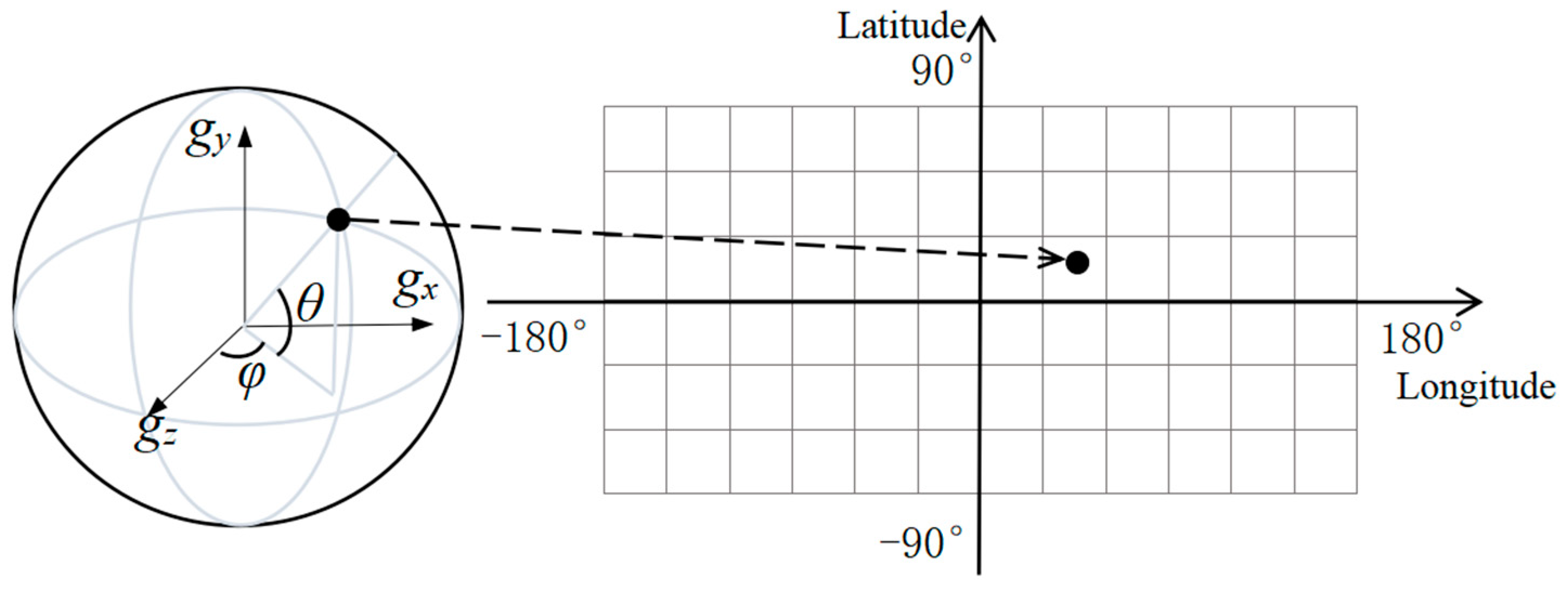
Incorporating spatial information into the extreme random trees model, which integrates the advantages of machine learning methods and spatial features, enhancing the predictive performance of the model. This model can offer novel approaches for the high-resolution reconstruction of diverse geographical data.
(2)
Utilizing the constructed model to reconstruct a 1 km high-resolution XCO2 dataset for China from 2016 to 2020.
(3)
Based on the predicted results, identifying and analyzing the spatiotemporal patterns of XCO2 within the Chinese region. These long-term, high-resolution XCO2 data contribute to our understanding of the spatiotemporal distribution characteristics of and variations in XCO2, thus improving the formulation of policies and strategies for carbon emission reduction.

2. Materials and Methods
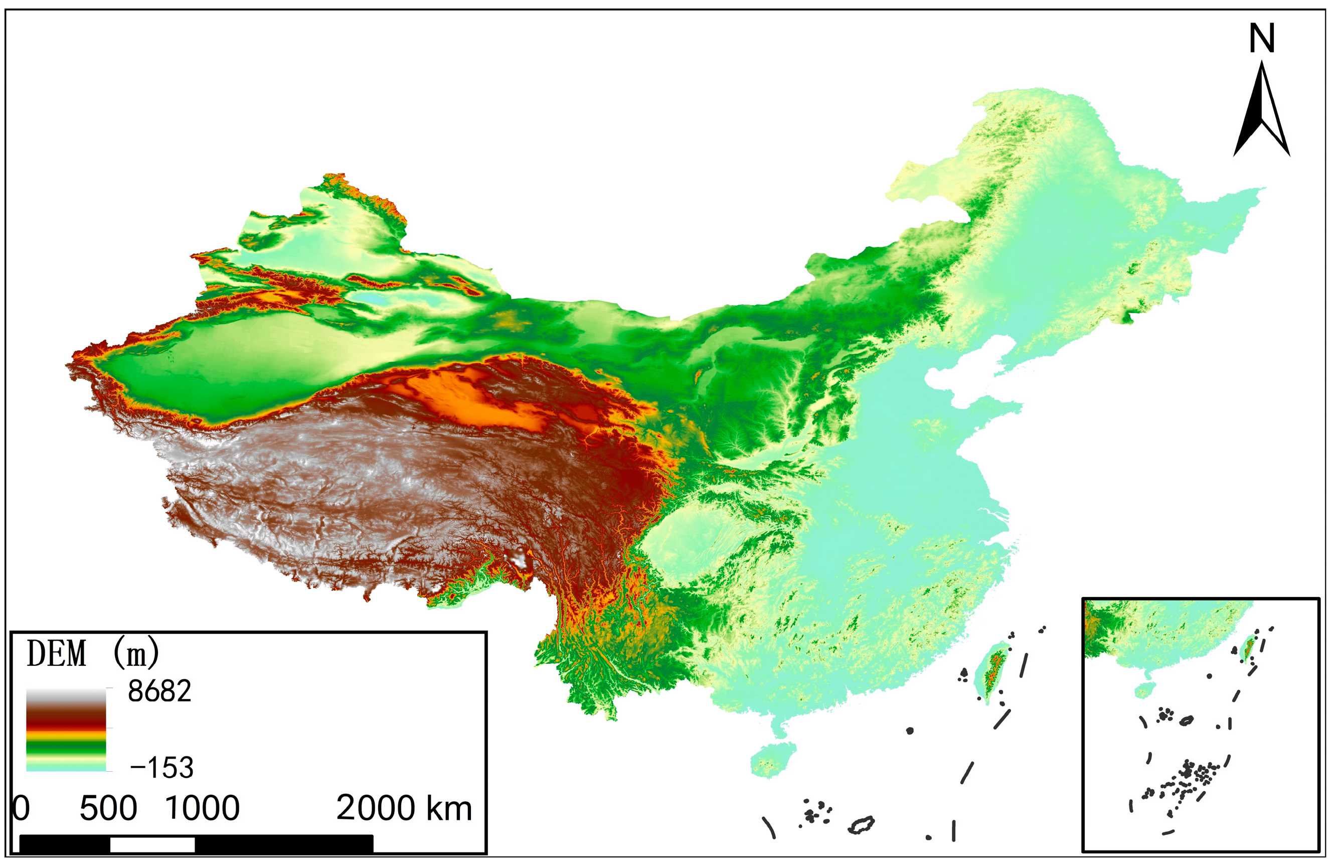
2.1. Study Area

We aimed to reconstruct the XCO2 data of the Chinese region (as shown in Figure 1) at high resolution. With a vast land area and diverse geographical environments, China, as the world’s second-largest economy, significantly influences global greenhouse gas emissions. China exhibits diverse terrain, including mountains, plateaus, plains, basins, and hills. Additionally, China’s climate types encompass tropical, subtropical, temperate, and cold temperate regions, showing distinct regional differences. These topographical and climatic features have significant impacts on the generation, transport, and distribution of carbon dioxide. For instance, mountainous regions may have lower carbon dioxide concentrations, while plain areas, due to dense populations and frequent industrial activities, may exhibit higher carbon dioxide emissions. Therefore, by conducting a more in-depth study to understand the spatial distribution and temporal trends of carbon dioxide concentrations in China, we can gain better insights into carbon cycle processes.

2.2. XCO2 Data

The XCO2 data used in this study were derived from a 2016–2020 global coverage XCO2 dataset generated by integrating multiple sources, including satellite data and reanalysis data [54]. Specifically, the dataset was generated by establishing the relationship between OCO-2 satellite XCO2 retrieval data and Copernicus Atmosphere Monitoring Service (CAMS) XCO2 reanalysis data with influencing factors such as NPP and RH using deep neural networks (DNNs). Subsequently, comprehensive XCO2 data were generated using CAMS XCO2 data and associated influencing factors. In this study, XCO2 data were modeled at a spatial resolution of 10 km. Therefore, following quality control, any null values and outliers in the dataset were removed to form the final XCO2 dataset at a resolution of 10 km.

2.3. Influencing Factors

Studies have shown that there are many factors that influence carbon dioxide concentration, among which population density (POP), temperature (TEM), normalized difference vegetation index (NDVI), precipitation (PRE), and gross primary productivity (GPP) are important factors affecting columnar carbon dioxide concentration (XCO2) [55,56]. In this study, we classified influencing factors into three categories: human activities, vegetation, and meteorological factors [57]. Areas with higher population density exhibit significantly higher carbon dioxide concentrations, as the distribution of emission sources such as industry and transportation directly affects carbon dioxide concentrations [58,59]. Vegetation conditions directly affect the absorption of carbon dioxide by vegetation and also influence the exchange processes between vegetation and the atmosphere. Meteorological factors such as temperature and precipitation also have significant effects on carbon dioxide concentrations. Therefore, in this study, factors related to human activities included population density (POP) and nighttime light index (NTL), vegetation conditions include gross primary productivity (GPP) and normalized difference vegetation index (NDVI), and meteorological conditions included temperature (TEM), precipitation (PRE), humidity (RH), and wind speed (WND). Additionally, we considered the influence of topography on carbon dioxide column concentration and incorporated digital elevation models (DEMs) for modeling purposes.
Population density has a significant impact on carbon dioxide (CO2) concentration. Regions with high population density are often associated with increased urbanization, industrialization, and commercial activities, which may lead to higher energy consumption and industrial emissions, thus increasing CO2 emissions [60,61]. The LandScan dataset used in this study is developed and maintained by the Oak Ridge National Laboratory (ORNL) of the Department of Energy (DOE) in the United States. It combines high-resolution satellite imagery, census data, geographic information system (GIS) data, and other geographical, topographical, and meteorological data, generated through complex models and algorithms, with a spatial resolution of 1 km [62]. The nighttime light (NTL) index is typically calculated using nighttime light images obtained from remote sensing satellites [63]. Its primary applications include urban planning, environmental monitoring, and economic development research. By measuring and recording the brightness of the Earth’s surface, nighttime light images can reveal the population density, level of economic activity, and urban development of an area. A high NTL index may indicate a higher level of economic development in the area, accompanied by increased energy use and CO2 emissions [64]. The NTL data used in this study were obtained from the VIIRS sensor on the Suomi NPP satellite and processed to eliminate noise from different dimensions to obtain the final dataset.
NDVI can accurately reflect the vegetation cover status of the Earth’s surface, and previous studies have shown a significant negative correlation between NDVI and carbon dioxide concentration [65]. We utilized an annual vegetation index dataset based on uninterrupted time series derived from SPOT/VEGETATION NDVI satellite remote sensing, with a spatial resolution of 1 km [66]. The NDVI data were sourced from the Resource and Environmental Science Data Center [67]. Gross primary productivity (GPP) is commonly used to describe the total amount of photosynthesis performed by plants in terrestrial ecosystems. Photosynthesis is the process by which plants utilize sunlight to convert carbon dioxide and water into organic substances. This process enables plants to capture and store carbon dioxide from the atmosphere, making it crucial for the carbon cycle in the atmosphere. Therefore, monitoring and studying GPP can provide a better understanding of the absorption, fixation, and release of carbon by plant ecosystems, which is important for understanding carbon dioxide concentration. The GPP data used in this study are sourced from the Global Ecology Group website and have a spatial resolution of 5 km [68].
Meteorological factors, such as temperature and precipitation, may impact the carbon cycle of terrestrial ecosystems and soil respiration [69]. Humidity impacts plant transpiration, affecting the rate at which plants absorb carbon dioxide [70]. Wind can disperse local gases, resulting in relatively lower carbon dioxide concentrations in localized areas [71]. The precipitation and temperature data used in this study are sourced from publicly available datasets at the National Earth System Science Data Center [72], while the humidity and wind speed datasets are from the Resource and Environmental Science Data Center [73]. The detailed information and sources of the selected independent variables are shown in Table 1.

2.4. Data Processing

In this study, our aim was to estimate the XCO2 in China at a spatial resolution of 1 km annually from 2016 to 2020. Therefore, we employed the nearest-neighbor interpolation method to resample all the aforementioned influencing factor data, ensuring they had a consistent spatial resolution of 1 km. Subsequently, we conducted quality control on the resampled influencing factor dataset, removing outliers and missing values. Then, we aggregated the quality-controlled 1 km influencing factor data by year, resulting in five 1 km input datasets for model prediction from 2016 to 2020. Next, we projected the 1 km influencing factor datasets onto the WGS84 projection coordinate system, resampled the 1 km resolution factors to a 10 km resolution using the nearest-neighbor method, and spatially matched the results with the original resolution of the XCO2 data (i.e., 10 km × 10 km) to generate training sample datasets. We obtained a total of 469,685 sample data points during the period from 2016 to 2020, with a spatial resolution of 10 km. Subsequently, we conducted modeling using the processed training sample dataset.

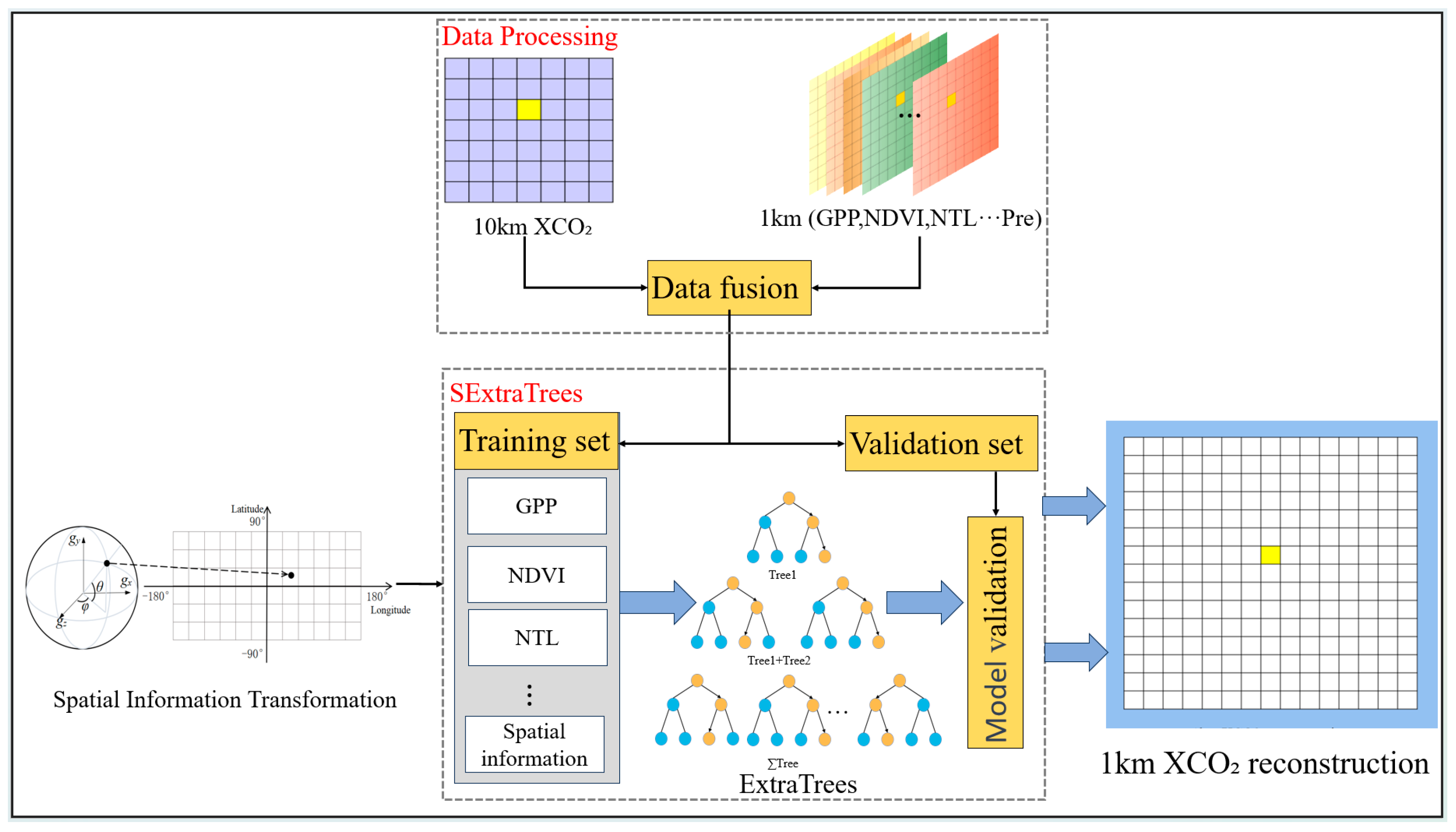
2.5. Spatial Extreme Random Trees

China is a vast territory, with significant differences in urbanization levels, industrial conditions, energy structures, and climate conditions among different regions, resulting in typical spatial distribution patterns of carbon dioxide concentration. There is evident spatial heterogeneity between carbon dioxide concentration and influencing factors. Although the extreme random trees method can increase the randomness and diversity of models and reduce the risk of overfitting by randomizing feature selection and threshold selection processes, better capture the nonlinear relationships between data, and further improve the robustness of the model, it cannot effectively address the spatial heterogeneity of XCO2. Therefore, by considering spatial features and incorporating spatial information into the extreme random trees model, we can inherit the advantages of extreme random trees and effectively address the uneven changes in geographical and temporal location characteristics. In this study, by adopting a geographic spatial encoding strategy (Equation (1)), latitude and longitude polar coordinates were converted into Cartesian coordinates in a three-dimensional Cartesian coordinate system to characterize the positional characteristics of geographical elements (Figure 2), resulting in feature variables that uniformly change within the range [−6371, 6371], i.e., spatial relationships. This spatial information exhibits smooth and uniform changes, effectively addressing the spatial heterogeneity issue of XCO2.
g i = g x i g y i g z i = R s i n φ i c o s θ i R s i n θ i R c o s φ i c o s θ i
In the equation, g i represents the geographic spatial information encoding feature of point i, φ i represents the longitude of point i,   θ i represents the latitude of point i, and R represents the radius of the Earth (approximately 6371 km).
The spatial extreme random trees model was used to establish the relationship between XCO2 and influencing factors at a resolution of 10 km. The specific principles of the spatial extreme random trees are illustrated in Figure 3. Initially, the pre-processed annual scale environmental factor data set with a spatial resolution of 1 km from 2016 to 2020 was resampled to an annual scale data set with a spatial resolution of 10 km by the nearest neighbor method, and aligned with the original XCO2 annual scale data set with a spatial resolution of 10 km. The XCO2 data of each point has corresponding environmental factor data, which establishes the corresponding relationship between the model-independent variables and some dependent variables, and this process is called data fusion. Subsequently, spatial information computed based on latitude and longitude was aggregated into the aligned dataset to form a training dataset. The model computation for the relationship between independent variables and dependent variables based on the spatial extreme random trees is represented by Equation (2). XCO2 data serve as the dependent variable, while factors such as DEM, GPP, and spatial features are used as independent variables for modeling. Leveraging this established relationship, the dataset of influencing factors at 1 km resolution was inputted into the trained spatial extreme random trees model to reconstruct China’s high-resolution (1 km) XCO2 dataset.
X C O 2 = S E x t r a T r e e s D E M , G P P , N D V I , N T L , P O P , W n d , P r e , T e m , R h , S p a t i a l   F e a t u r e s                  
To validate the performance of the spatial extreme random trees method in reconstructing XCO2, we selected mainstream downscaling methods such as Kriging interpolation and extreme random trees for comparison and analyzed the results of resolution reconstruction using various methods. We employed the 10-fold cross-validation method to evaluate the performance of the spatial extreme random trees. The original dataset was randomly partitioned into ten equally sized subsets, nine of which were allocated for training the model, while the remaining segment was designated for validating the model’s performance. The best model parameters were determined through ten-fold cross-validation. The performance of the established models was evaluated using three evaluation metrics: mean absolute error (MAE), root-mean-squared error (RMSE), and coefficient of determination (R2). The calculation of these statistical metrics can be achieved as follows:
RMSE = 1 n i = 1 n y i y i ^ 2
MAE = 1 n i = 1 n | y i y i ^ |
R 2 = 1 i = 1 n ( y i y i ^ ) 2 i = 1 n ( y i y i ¯ ) 2
In this context, n stands for the sample size; y i and y i ^ denote the observed XCO2 value and the predicted XCO2 value for sample i, respectively; and y i ¯ represents the average of the observed XCO2 values.

3. Results

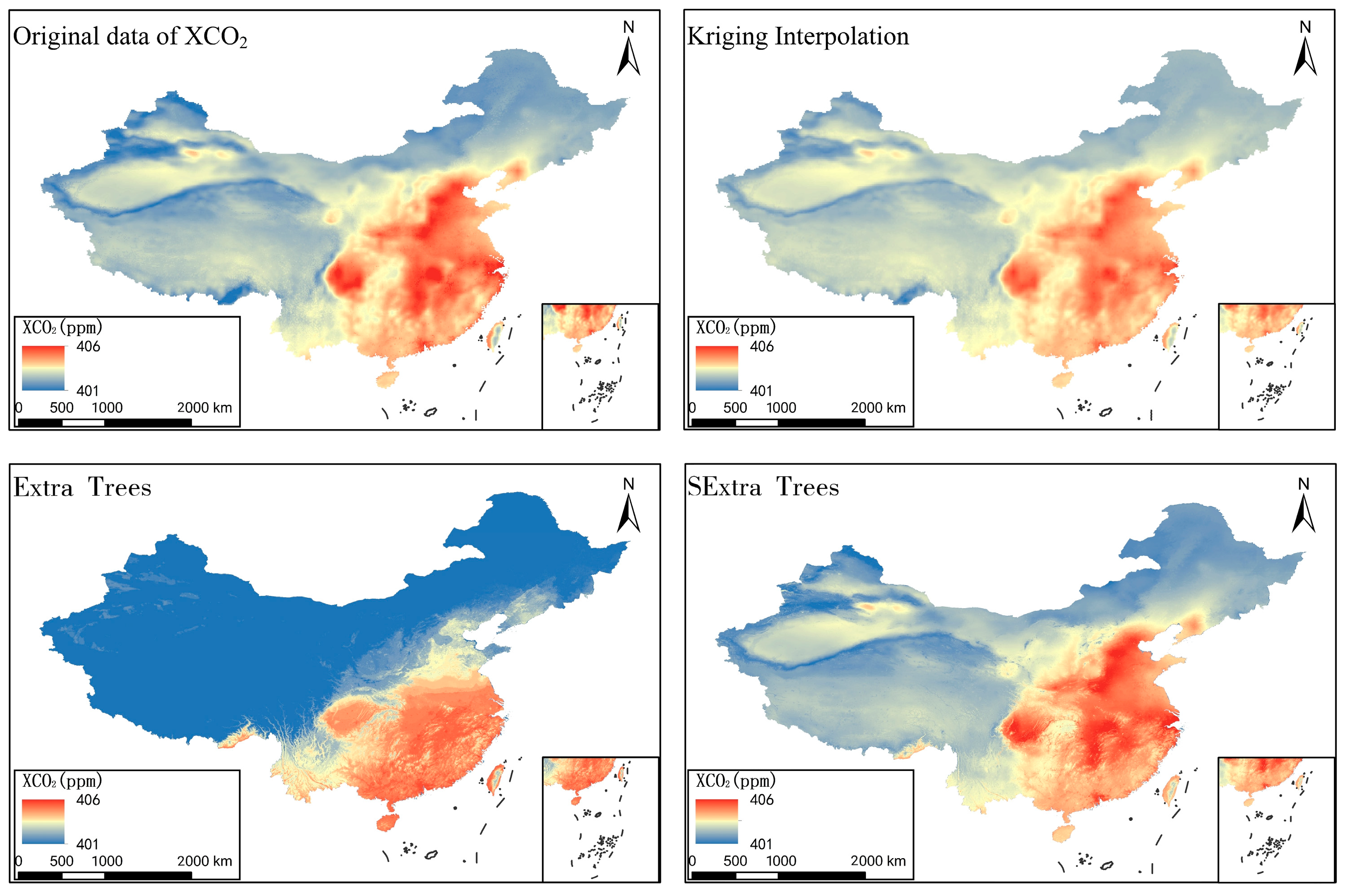
3.1. Model Comparison

To assess the effectiveness of the proposed model, we compared the predictive results of the spatial extreme random trees model with those of Kriging interpolation and extreme random trees model predictions. The fitting results of each model are shown in Table 2. Kriging interpolation, as the most classical interpolation method, infers values at unknown locations by leveraging the spatial correlation between known observation points. Previous studies have demonstrated its effectiveness in CO2-related research [37]. Since the data initially used for this method are XCO2 data with a resolution of 10 km, and the known points are evenly distributed, the fitting results are relatively good, with an R2 of 0.961, MAE of 0.697 ppm, and RMSE of 0.699 ppm. However, this method can only model and interpolate single variables, which ignores the spatiotemporal correlation between XCO2 and other influencing factors. It may oversmooth the data, fail to capture local variability, exhibit a poor ability to predict nonlinear relationships, and have low efficiency and accuracy when computing large amounts of data. Although the extreme random trees model considers the complex relationships between XCO2 and other influencing factors and performs well in capturing nonlinear relationships and improving efficiency when processing large amounts of data, it ignores the spatial heterogeneity of XCO2. The fitting results for the extreme random trees model are as follows: R2 = 0.939, MAE = 0.726 ppm, and RMSE = 0.866 ppm. In contrast, the spatial extreme random trees model demonstrates strong nonlinear modeling capabilities. When spatial features were integrated into the machine learning method, this model’s ability to capture spatial geographical relationships was enhanced, leading to significantly improved fitting accuracy with an R2 of 0.985, MAE of 0.407 ppm, and RMSE of 0.434 ppm. Hence, we opted to employ spatial extreme random trees for the high-resolution reconstruction of XCO2.
Figure 4 illustrates the spatial distribution of the initial XCO2 data at a 10 km resolution in 2016, along with the reconstructed XCO2 results at a 1 km resolution using different methods. Because Kriging interpolation infers the values at unknown points based on the numerical values of known points, and XCO2 generally exhibits a gradual trend, visually, the Kriging interpolation results show a clear smoothing trend. By ignoring spatial heterogeneity, the extreme random trees model theoretically underestimates the complexity of XCO2 spatial distribution, leading to the phenomenon of underestimation in the predicted XCO2 values, particularly in eastern coastal areas. The spatial distribution of XCO2 predicted by the spatial extreme random trees model is most similar to the original data, indicating that our reconstructed XCO2 data possess higher precision and accuracy.

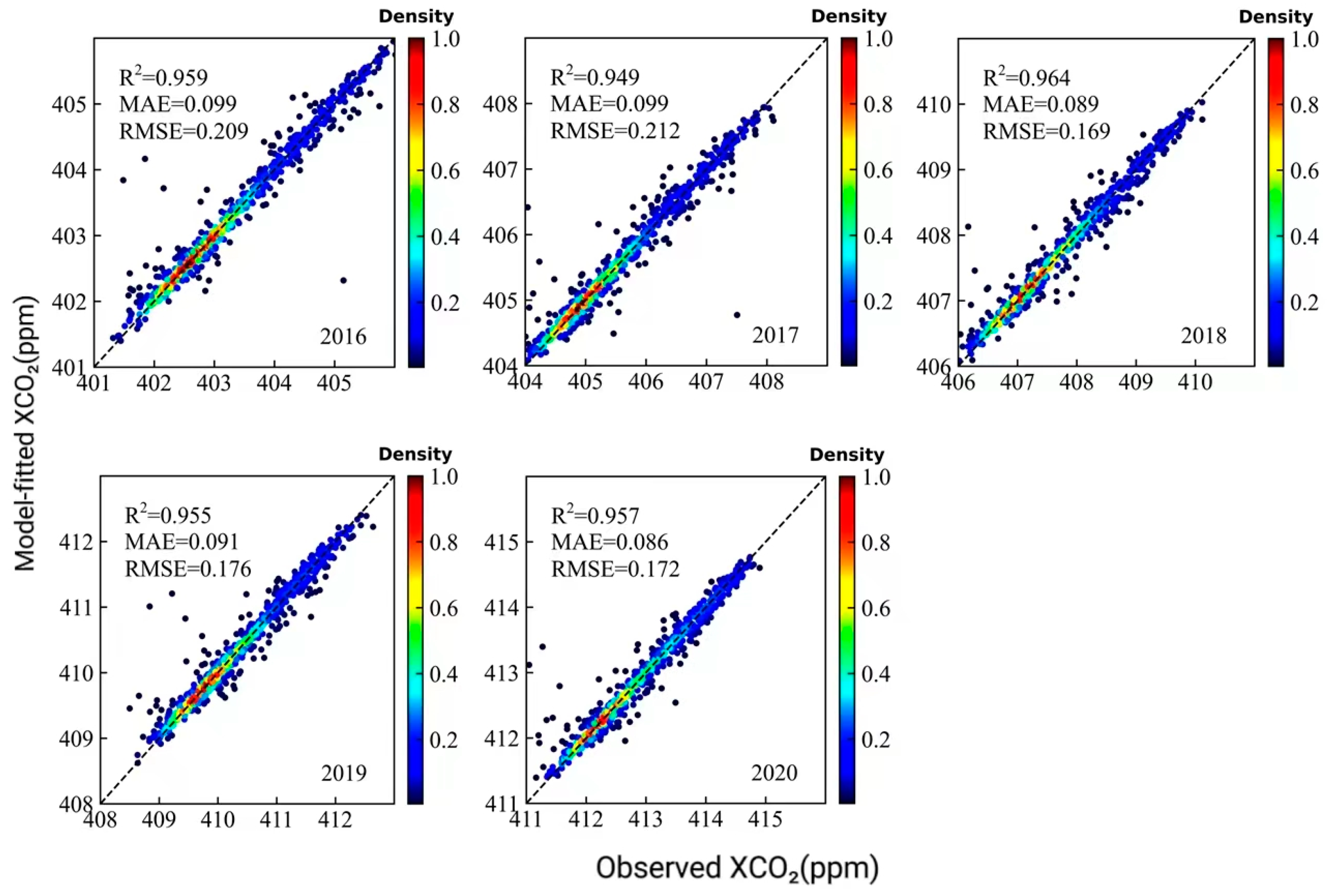
3.2. Spatial Extreme Random Trees Validation

In this study, based on the spatial extreme random trees model, the 10 km-resolution XCO2 spatiotemporal dataset for China from 2016 to 2020 was reconstructed at a 1 km resolution. The model fitting results for each year are depicted in Figure 5. The fitting R2 values range from 0.949 (2017) to 0.964 (2018), indicating high precision in both RMSE and MAE results. The accuracy of the prediction results demonstrates that the spatial extreme random trees model can reliably predict XCO2 at relatively fine resolutions.

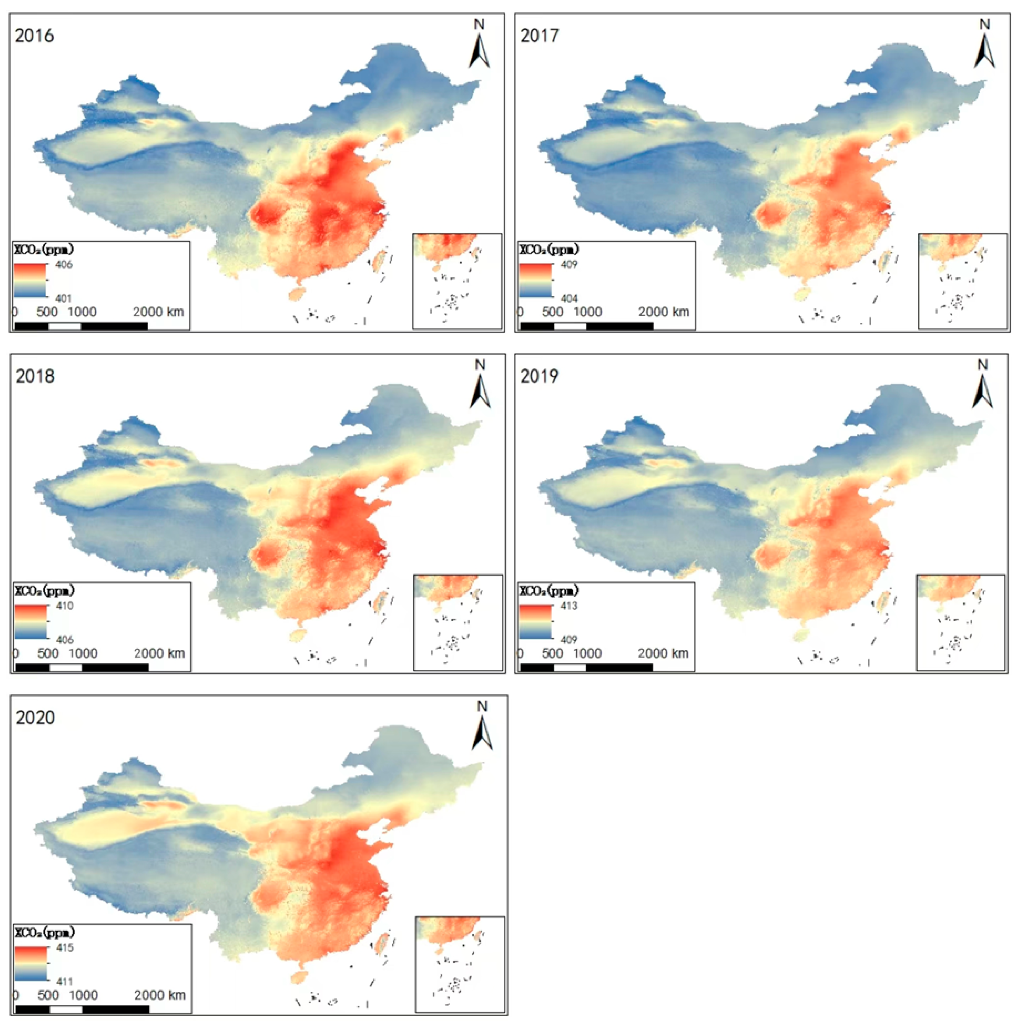
3.3. Spatiotemporal Variations in XCO2 in China

The results of China’s 1 km-resolution XCO2 spatiotemporal dataset reconstructed using spatial extreme random trees from 2016 to 2020 are shown in Figure 6, indicating notable spatial variations in the distribution of XCO2. Overall, consistent with the existing research results, the carbon dioxide concentration tends to be relatively lower in western China and higher in eastern China, a pattern that aligns with the level of urbanization and economic development in China [74]. The rapid urbanization in China from 2016 to 2020 has led to significant differences in XCO2 between developed eastern regions and underdeveloped western regions. The eastern regions of China are typically characterized by economic prosperity, dense population, and intensive energy and industrial activities, which may result in higher carbon dioxide concentrations. Cities such as Beijing, Shanghai, and parts of Jiangsu province often exhibit higher population densities, traffic volumes, and industrial activities, leading to higher carbon dioxide concentrations in urban areas. In contrast, the western and northeastern regions of China may be more influenced by natural factors. Regions with high vegetation coverage, such as Tibet, Inner Mongolia, and Heilongjiang, absorb more carbon dioxide through plant photosynthesis, resulting in lower carbon dioxide concentrations. Additionally, the western regions have lower population densities and are gradually transitioning from traditional to new energy sources (such as wind and solar energy), thus reducing carbon emissions. The economy in the southwestern and southern regions is relatively developed, with extensive human activities. However, because of the warm and humid climate prevailing in these regions, vegetation is lush, resulting in the higher efficiency of carbon fixation through photosynthesis. Therefore, the XCO2 level is moderate [75]. Further, optimizing the energy structure and improving energy efficiency to decrease carbon intensity, as well as increasing vegetation coverage to enhance carbon sequestration, are effective approaches for reducing or mitigating XCO2. The 1 km-resolution XCO2 data reconstructed via spatial extreme random trees can achieve comprehensive coverage with high resolution in China, thereby enabling more effective monitoring of carbon sources and sinks.
The spatial distribution of XCO2 trends in China from 2016 to 2020, as shown in Figure 7, is consistent with the global trend, with an overall increase in XCO2 levels nationwide each year [76]. Specifically, all regions exhibit significant increments, with an average annual rise of over 1.88 ppm/year over the past five years. The rate of XCO2 growth varies across regions. In the northwest, northeast, and northern parts of China, the concentration of carbon dioxide in the atmosphere has increased rapidly, with XCO2 levels higher than the five-year average. This could be attributed to accelerated urbanization in China, intensive human activities, and increased energy consumption that have led to higher carbon emissions. In contrast, although XCO2 levels in southwest, central, eastern, and southern China have increased annually, the growth rates have been relatively slow. For example, XCO2 levels increased more slowly near cities such as Chengdu, Chongqing, Changsha, and Wuhan. This may be due to the rapid economic development, high population density, and high level of urbanization in these regions, which emit more carbon dioxide, resulting in a large carbon dioxide concentration base and in a lower growth rate in these regions. Additionally, the warm and humid climate in the southern regions supports lush vegetation, which efficiently absorbs carbon dioxide through photosynthesis, mitigating the increase in atmospheric carbon dioxide. Moreover, eastern and southern regions of China have gradually transitioned from energy-intensive economic growth to green and sustainable development, which may have contributed to the slowdown in XCO2 growth rates. When studying the spatiotemporal distribution of XCO2, it is crucial to consider the non-uniformity of carbon dioxide emissions. Therefore, obtaining long-term, high-resolution XCO2 data can provide a scientific basis for China to formulate reasonable carbon emission reduction policies. To better assess carbon emissions within China, reasonable CO2 emission analyses are needed across different regions.

4. Conclusions

As CO2 is a major greenhouse gas, excessive CO2 emissions are a significant contributor to global warming. In this study, we introduced a novel spatial downscaling model named SExtraTrees, aimed at addressing the research gap in reconstructing high-resolution XCO2 from the perspective of spatial heterogeneity. By considering nonlinear relationships and spatial characteristics, SExtraTrees further enhances the accuracy and robustness of high-resolution XCO2 reconstruction, thereby improving the model’s generalizability. Based on XCO2 data with a spatial resolution of 10 km from 2016 to 2020, we successfully reconstructed XCO2 at a spatial resolution of 1 km. To meet the need for carbon emission monitoring, the spatiotemporal characteristics of XCO2 were analyzed within the region of China. Based on the results of this study, the following conclusions were drawn:
(1)
The SExtraTrees model proposed in this study is an effective technique for predicting national long-term time series XCO2 data. The SExtraTrees model outperforms Kriging interpolation and extreme random trees models in terms of model fitting and prediction while maintaining spatial consistency with the original XCO2 data and ensuring high predictive accuracy.
(2)
The 1 km-resolution XCO2 products reconstructed using the spatial extreme random trees model provide fundamental data and technical support for regional XCO2 monitoring. These predicted XCO2 datasets can also serve as a reference for calibrating other low-resolution XCO2 datasets. The obtained results highlight the importance of combining geographic spatial correlations with machine learning methods to achieve high precision and robustness. The spatial extreme random trees model can also be applied to the resolution reconstruction of other environmental factors.
(3)
Based on the resolution reconstruction results of the spatial extreme random trees model, XCO2 exhibits significant spatial and temporal heterogeneity. From 2016 to 2020, XCO2 in China shows an increasing trend each year. Nationally, the spatial distribution of XCO2 aligns with China’s economic development and urbanization level, with higher XCO2 concentrations in the eastern regions and lower concentrations in the western regions of China. The distribution of carbon concentrations varies among different regions, mainly due to differences in the geographical environment, economic development level, and industrial structure. Higher vegetation coverage can enhance the carbon sequestration capacity. Given the spatiotemporal changes and differences in XCO2, this study provides scientific references for reducing carbon emissions, which is essential for crafting efficient policies aimed at reducing carbon emissions and addressing climate change.
In summary, the spatial extreme random trees model enhances the fitting capability of XCO2 with complex spatial features and exhibits good generalization performance. SExtraTrees may also be applicable to other studies related to high-resolution reconstruction of air pollutants, serving as a methodological reference for reconstructing other factors at high resolutions. It is worth noting that in other relevant studies, when establishing models, it is essential to select influential factors that are strongly correlated with the dependent variable. Through the application of the spatial extreme random trees model, we have gained deeper insights into the spatiotemporal distribution characteristics of XCO2 in China, providing robust data support for future carbon emission control and climate change research. In future studies, it will be necessary to further consider the unique temporal characteristics of XCO2 data. Additionally, given the diverse and complex environmental factors influencing XCO2, there is a necessity for more in-depth research into the intricate relationships between influencing factors and XCO2. By employing spatial statistical analysis and time series analysis, we aim to thoroughly explore the spatiotemporal information embedded in long time series CO2 satellite observations, meteorological station data, and other relevant datasets. By integrating data from various time points and spatial locations, we seek to acquire a more comprehensive and holistic understanding of spatiotemporal dynamics, thereby continuously enhancing the resolution reconstruction models for XCO2 data.

Author Contributions

Conceptualization, X.L. and S.J.; methodology, S.J.; software, T.W.; validation, X.L., S.J., and S.Z.; formal analysis, T.W.; investigation, S.J.; resources, T.W.; data curation, X.L.; writing—original draft preparation, X.W.; writing—review and editing, D.J.; visualization, X.L.; supervision, X.L.; project administration, J.G.; funding acquisition, T.W. All authors have read and agreed to the published version of the manuscript.

Funding

This research was funded by the Jiangsu Province Ecological Environment Monitoring Fund (project number: 2216) and the Common Application Support Platform for National Civil Space Infrastructure Land Observation Satellites (grant number: 2017-000052-73-01-001735).

Institutional Review Board Statement

Not applicable.

Informed Consent Statement

Not applicable.

Data Availability Statement

The XCO2 dataset used in this article can be obtained from the following link: (https://doi.org/10.5281/zenodo.7793917 (accessed on 10 February 2024)). The DEM, NDVI, WND, and RH data were collected from the Chinese Academy of Sciences Resource and Environment Science and Data Center via the following link: (https://www.resdc.cn (accessed on 10 February 2024)). The TEM and PRE data used in this article were sourced from the National Earth System Science Data Center. The data can be accessed through the following link: (http://loess.geodata.cn/ (accessed on 10 February 2024)). The GPP data were obtained from the Global Ecology Group and can be accessed via the following link: (https://globalecology.unh.edu/ (accessed on 10 February 2024)); the NTL data were obtained from the Institute of Remote Sensing and Digital Earth, Chinese Academy of Sciences, and can be accessed via the following link: (https://www.zybuluo.com/novachen/note/1162587 (accessed on 10 February 2024)); and the POP data were obtained from Oak Ridge National Laboratory and can be accessed at the following link: (https://landscan.ornl.gov/ (accessed on 10 February 2024)).

Conflicts of Interest

The authors declare no conflicts of interest.

References

  1. Caminade, C.; McIntyre, K.M.; Jones, A.E. Impact of recent and future climate change on vector-borne diseases. Ann. N. Y. Acad. Sci. 2019, 1436, 157–173. [Google Scholar] [CrossRef] [PubMed]
  2. Hao, Y.; Chen, H.; Wei, Y.-M.; Li, Y.-M. The influence of climate change on CO2 (carbon dioxide) emissions: An empirical estimation based on Chinese provincial panel data. J. Clean. Prod. 2016, 131, 667–677. [Google Scholar] [CrossRef]
  3. Quadrelli, R.; Peterson, S. The energy–climate challenge: Recent trends in CO2 emissions from fuel combustion. Energy Policy 2007, 35, 5938–5952. [Google Scholar] [CrossRef]
  4. Montzka, S.A.; Dlugokencky, E.J.; Butler, J.H. Non-CO2 greenhouse gases and climate change. Nature 2011, 476, 43–50. [Google Scholar] [CrossRef] [PubMed]
  5. Holland, D.M.; Thomas, R.H.; de Young, B.; Ribergaard, M.H.; Lyberth, B. Acceleration of Jakobshavn Isbræ triggered by warm subsurface ocean waters. Nat. Geosci. 2008, 1, 659–664. [Google Scholar] [CrossRef]
  6. Sellers, P.J.; Schimel, D.S.; Moore, B., 3rd; Liu, J.; Eldering, A. Observing carbon cycle-climate feedbacks from space. Proc. Natl. Acad. Sci. USA 2018, 115, 7860–7868. [Google Scholar] [CrossRef] [PubMed]
  7. Solomon, S.; Plattner, G.-K.; Knutti, R.; Friedlingstein, P. Irreversible climate change due to carbon dioxide emissions. Proc. Natl. Acad. Sci. USA 2009, 106, 1704–1709. [Google Scholar] [CrossRef] [PubMed]
  8. Scholze, M.; Knorr, W.; Arnell, N.W.; Prentice, I.C. A climate-change risk analysis for world ecosystems. Proc. Natl. Acad. Sci. USA 2006, 103, 13116–13120. [Google Scholar] [CrossRef] [PubMed]
  9. Yu, K.M.; Curcic, I.; Gabriel, J.; Tsang, S.C. Recent advances in CO2 capture and utilization. ChemSusChem 2008, 1, 893–899. [Google Scholar] [CrossRef] [PubMed]
  10. Yu, C.-H.; Huang, C.-H.; Tan, C.-S. A Review of CO2 Capture by Absorption and Adsorption. Aerosol Air Qual. Res. 2012, 12, 745–769. [Google Scholar] [CrossRef]
  11. Jimenez, V.; Ramirez-Lucas, A.; Diaz, J.A.; Sanchez, P.; Romero, A. CO2 capture in different carbon materials. Environ. Sci. Technol. 2012, 46, 7407–7414. [Google Scholar] [CrossRef] [PubMed]
  12. Ajayi, T.; Gomes, J.S.; Bera, A. A review of CO2 storage in geological formations emphasizing modeling, monitoring and capacity estimation approaches. Pet. Sci. 2019, 16, 1028–1063. [Google Scholar] [CrossRef]
  13. Labzovskii, L.D.; Mak, H.W.L.; Takele Kenea, S.; Rhee, J.-S.; Lashkari, A.; Li, S.; Goo, T.-Y.; Oh, Y.-S.; Byun, Y.-H. What can we learn about effectiveness of carbon reduction policies from interannual variability of fossil fuel CO2 emissions in East Asia? Environ. Sci. Policy 2019, 96, 132–140. [Google Scholar] [CrossRef]
  14. Potier, E.; Broquet, G.; Wang, Y.; Santaren, D.; Berchet, A.; Pison, I.; Marshall, J.; Ciais, P.; Bréon, F.-M.; Chevallier, F. Complementing XCO2 imagery with ground-based CO2 and 14CO2 measurements to monitor CO2 emissions from fossil fuels on a regional to local scale. Atmos. Meas. Tech. 2022, 15, 5261–5288. [Google Scholar] [CrossRef]
  15. Rothenberg, G. A realistic look at CO2 emissions, climate change and the role of sustainable chemistry. Sustain. Chem. Clim. Action 2023, 2, 100012. [Google Scholar] [CrossRef]
  16. Finkbeiner, M.; Bach, V. Life cycle assessment of decarbonization options—Towards scientifically robust carbon neutrality. Int. J. Life Cycle Assess. 2021, 26, 635–639. [Google Scholar] [CrossRef]
  17. Gil, L.; Bernardo, J. An approach to energy and climate issues aiming at carbon neutrality. Renew. Energy Focus 2020, 33, 37–42. [Google Scholar] [CrossRef]
  18. Ciais, P.; Dolman, A.J.; Bombelli, A.; Duren, R.; Peregon, A.; Rayner, P.J.; Miller, C.; Gobron, N.; Kinderman, G.; Marland, G.; et al. Current systematic carbon-cycle observations and the need for implementing a policy-relevant carbon observing system. Biogeosciences 2014, 11, 3547–3602. [Google Scholar] [CrossRef]
  19. Wunch, D.; Toon, G.C.; Blavier, J.F.; Washenfelder, R.A.; Notholt, J.; Connor, B.J.; Griffith, D.W.; Sherlock, V.; Wennberg, P.O. The total carbon column observing network. Philos. Trans. A Math. Phys. Eng. Sci. 2011, 369, 2087–2112. [Google Scholar] [CrossRef]
  20. Chevallier, F.; Deutscher, N.M.; Conway, T.J.; Ciais, P.; Ciattaglia, L.; Dohe, S.; Fröhlich, M.; Gomez-Pelaez, A.J.; Griffith, D.; Hase, F.; et al. Global CO2fluxes inferred from surface air-sample measurements and from TCCON retrievals of the CO2total column. Geophys. Res. Lett. 2011, 38. [Google Scholar] [CrossRef]
  21. Heiskanen, J.; Brümmer, C.; Buchmann, N.; Calfapietra, C.; Chen, H.; Gielen, B.; Gkritzalis, T.; Hammer, S.; Hartman, S.; Herbst, M.; et al. The Integrated Carbon Observation System in Europe. Bull. Am. Meteorol. Soc. 2022, 103, E855–E872. [Google Scholar] [CrossRef]
  22. Shiga, Y.P.; Michalak, A.M.; Randolph Kawa, S.; Engelen, R.J. In-situ CO2 monitoring network evaluation and design: A criterion based on atmospheric CO2 variability. J. Geophys.Res. Atmos. 2013, 118, 2007–2018. [Google Scholar] [CrossRef]
  23. Siabi, Z.; Falahatkar, S.; Alavi, S.J. Spatial distribution of XCO(2) using OCO-2 data in growing seasons. J. Environ. Manag. 2019, 244, 110–118. [Google Scholar] [CrossRef]
  24. Pan, G.; Xu, Y.; Ma, J. The potential of CO(2) satellite monitoring for climate governance: A review. J. Environ. Manag. 2021, 277, 111423. [Google Scholar] [CrossRef] [PubMed]
  25. Wang, Y.; Wang, M.; Teng, F.; Ji, Y. Remote Sensing Monitoring and Analysis of Spatiotemporal Changes in China’s Anthropogenic Carbon Emissions Based on XCO2 Data. Remote Sens. 2023, 15, 3207. [Google Scholar] [CrossRef]
  26. Lu, S.; Wang, J.; Wang, Y.; Yan, J. Analysis on the variations of atmospheric CO2 concentrations along the urban–rural gradients of Chinese cities based on the OCO-2 XCO2 data. Int. J. Remote Sens. 2018, 39, 4194–4213. [Google Scholar] [CrossRef]
  27. Hakkarainen, J.; Ialongo, I.; Maksyutov, S.; Crisp, D. Analysis of Four Years of Global XCO2 Anomalies as Seen by Orbiting Carbon Observatory-2. Remote Sens. 2019, 11, 850. [Google Scholar] [CrossRef]
  28. Cogan, A.J.; Boesch, H.; Parker, R.J.; Feng, L.; Palmer, P.I.; Blavier, J.F.L.; Deutscher, N.M.; Macatangay, R.; Notholt, J.; Roehl, C.; et al. Atmospheric carbon dioxide retrieved from the Greenhouse gases Observing SATellite (GOSAT): Comparison with ground-based TCCON observations and GEOS-Chem model calculations. J. Geophys. Res. Atmos. 2012, 117, D21. [Google Scholar] [CrossRef]
  29. Crisp, D.; Pollock, H.R.; Rosenberg, R.; Chapsky, L.; Lee, R.A.M.; Oyafuso, F.A.; Frankenberg, C.; O’Dell, C.W.; Bruegge, C.J.; Doran, G.B.; et al. The on-orbit performance of the Orbiting Carbon Observatory-2 (OCO-2) instrument and its radiometrically calibrated products. Atmos. Meas. Tech. 2017, 10, 59–81. [Google Scholar] [CrossRef]
  30. Sheng, M.; Lei, L.; Zeng, Z.-C.; Rao, W.; Song, H.; Wu, C. Global land 1° mapping dataset of XCO2 from satellite observations of GOSAT and OCO-2 from 2009 to 2020. Big Earth Data 2022, 7, 170–190. [Google Scholar] [CrossRef]
  31. Liu, Y.; Wang, J.; Yao, L.; Chen, X.; Cai, Z.; Yang, D.; Yin, Z.; Gu, S.; Tian, L.; Lu, N.; et al. The TanSat mission: Preliminary global observations. Sci. Bull. 2018, 63, 1200–1207. [Google Scholar] [CrossRef] [PubMed]
  32. Kuhlmann, G.; Brunner, D.; Broquet, G.; Meijer, Y. Quantifying CO2 emissions of a city with the Copernicus Anthropogenic CO2 Monitoring satellite mission. Atmos. Meas. Tech. 2020, 13, 6733–6754. [Google Scholar] [CrossRef]
  33. Ruonan, P.; Liang, A.; Xinyü, L.; Xinjie, L.J.R.S.T. High Spatio-temporal Resolution XCO2 Data Interpolation Algorithm based on OCO-2/3 Satellite. Remote Sens. Technol. Appl. 2023, 38, 614–623. [Google Scholar]
  34. Jing, Y.; Shi, J.; Wang, T.; Sussmann, R. Mapping Global Atmospheric CO2 Concentration at High Spatiotemporal Resolution. Atmosphere 2014, 5, 870–888. [Google Scholar] [CrossRef]
  35. Zeng, Z.-C.; Lei, L.; Strong, K.; Jones, D.B.A.; Guo, L.; Liu, M.; Deng, F.; Deutscher, N.M.; Dubey, M.K.; Griffith, D.W.T.; et al. Global land mapping of satellite-observed CO2 total columns using spatio-temporal geostatistics. Int. J. Digit. Earth 2016, 10, 426–456. [Google Scholar] [CrossRef]
  36. Hammerling, D.M.; Michalak, A.M.; Kawa, S.R. Mapping of CO2 at high spatiotemporal resolution using satellite observations: Global distributions from OCO-2. J. Geophys.Res. Atmos. 2012, 117. [Google Scholar] [CrossRef]
  37. Mousavi, S.M.; Dinan, N.M.; Ansarifard, S.; Sonnentag, O. Analyzing spatio-temporal patterns in atmospheric carbon dioxide concentration across Iran from 2003 to 2020. Atmos.Environ. X 2022, 14, 100163. [Google Scholar] [CrossRef]
  38. Bhattacharjee, S.; Dill, K.; Chen, J. Forecasting Interannual Space-based CO2 Concentration using Geostatistical Mapping Approach. In Proceedings of the 2020 IEEE International Conference on Electronics, Computing and Communication Technologies (CONECCT), Bangalore, India, 2–4 July 2020; pp. 1–6. [Google Scholar]
  39. He, Z.; Lei, L.; Zhang, Y.; Sheng, M.; Wu, C.; Li, L.; Zeng, Z.-C.; Welp, L.R. Spatio-Temporal Mapping of Multi-Satellite Observed Column Atmospheric CO2 Using Precision-Weighted Kriging Method. Remote Sens. 2020, 12, 576. [Google Scholar] [CrossRef]
  40. Mousavi, S.M.; Dinan, N.M.; Ansarifard, S.; Borhani, F.; Ezimand, K.; Naghibi, A. Examining the Role of the Main Terrestrial Factors Won the Seasonal Distribution of Atmospheric Carbon Dioxide Concentration over Iran. J. Indian Soc. Remote Sens. 2023, 51, 865–875. [Google Scholar] [CrossRef]
  41. Golkar, F.; Mousavi, S.M. Variation of XCO2 anomaly patterns in the Middle East from OCO-2 satellite data. Int. J. Digit. Earth 2022, 15, 1219–1235. [Google Scholar] [CrossRef]
  42. Liang, A.; Pang, R.; Chen, C.; Xiang, C. XCO2 Fusion Algorithm Based on Multi-Source Greenhouse Gas Satellites and CarbonTracker. Atmosphere 2023, 14, 1335. [Google Scholar] [CrossRef]
  43. Zhao, Z.; Xie, F.; Ren, T.; Zhao, C. Atmospheric CO2retrieval from satellite spectral measurements by a two-step machine learning approach. J. Quant. Spectrosc. Radiat. Transf. 2022, 278, 108006. [Google Scholar] [CrossRef]
  44. Mohammadi, F.; Teiri, H.; Hajizadeh, Y.; Abdolahnejad, A.; Ebrahimi, A. Prediction of atmospheric PM(2.5) level by machine learning techniques in Isfahan, Iran. Sci. Rep. 2024, 14, 2109. [Google Scholar] [CrossRef] [PubMed]
  45. Mak, H.W.L. Improved Remote Sensing Algorithms and Data Assimilation Approaches in Solving Environmental Retrieval Problems; Hong Kong University of Science and Technology: Hong Kong, China, 2019. [Google Scholar]
  46. He, C.; Ji, M.; Li, T.; Liu, X.; Tang, D.; Zhang, S.; Luo, Y.; Grieneisen, M.L.; Zhou, Z.; Zhan, Y. Deriving Full-Coverage and Fine-Scale XCO2 Across China Based on OCO-2 Satellite Retrievals and CarbonTracker Output. Geophys. Res. Lett. 2022, 49, e2022GL098435. [Google Scholar] [CrossRef]
  47. Wang, W.; He, J.; Feng, H.; Jin, Z. High-Coverage Reconstruction of XCO(2) Using Multisource Satellite Remote Sensing Data in Beijing-Tianjin-Hebei Region. Int. J. Environ. Res. Public Health 2022, 19, 10853. [Google Scholar] [CrossRef] [PubMed]
  48. He, S.; Yuan, Y.; Wang, Z.; Luo, L.; Zhang, Z.; Dong, H.; Zhang, C. Machine Learning Model-Based Estimation of XCO2 with High Spatiotemporal Resolution in China. Atmosphere 2023, 14, 436. [Google Scholar] [CrossRef]
  49. Hastie, T.; Tibshirani, R.; Friedman, J. Random Forests. In The Elements of Statistical Learning; Springer Series in Statistics; Springer: Berlin/Heidelberg, Germany, 2009; pp. 1–18. [Google Scholar]
  50. Chen, T.; Guestrin, C. XGBoost. In Proceedings of the 22nd ACM SIGKDD International Conference on Knowledge Discovery and Data Mining, San Francisco, CA, USA, 13–17 August 2016; pp. 785–794. [Google Scholar]
  51. Cheng, J.; Li, G.; Chen, X. Research on Travel Time Prediction Model of Freeway Based on Gradient Boosting Decision Tree. IEEE Access 2019, 7, 7466–7480. [Google Scholar] [CrossRef]
  52. Geurts, P.; Ernst, D.; Wehenkel, L. Extremely randomized trees. Mach. Learn. 2006, 63, 3–42. [Google Scholar] [CrossRef]
  53. Wu, C.; Ju, Y.; Yang, S.; Zhang, Z.; Chen, Y. Reconstructing annual XCO(2) at a 1 kmx1 km spatial resolution across China from 2012 to 2019 based on a spatial CatBoost method. Environ Res 2023, 236, 116866. [Google Scholar] [CrossRef]
  54. Li, T.; Wu, J.; Wang, T. Generating daily high-resolution and full-coverage XCO(2) across China from 2015 to 2020 based on OCO-2 and CAMS data. Sci. Total Environ. 2023, 893, 164921. [Google Scholar] [CrossRef]
  55. Li, H.; Mu, H.; Zhang, M.; Li, N. Analysis on influence factors of China’s CO2 emissions based on Path–STIRPAT model. Energy Policy 2011, 39, 6906–6911. [Google Scholar] [CrossRef]
  56. Liu, K.; Xue, M.; Peng, M.; Wang, C. Impact of spatial structure of urban agglomeration on carbon emissions: An analysis of the Shandong Peninsula, China. Technol. Forecast. Soc. Chang. 2020, 161, 120313. [Google Scholar] [CrossRef]
  57. Dong, K.; Hochman, G.; Zhang, Y.; Sun, R.; Li, H.; Liao, H. CO2 emissions, economic and population growth, and renewable energy: Empirical evidence across regions. Energy Econ. 2018, 75, 180–192. [Google Scholar] [CrossRef]
  58. Sun, H.; Li, M.; Xue, Y. Examining the Factors Influencing Transport Sector CO2 Emissions and Their Efficiency in Central China. Sustainability 2019, 11, 4712. [Google Scholar] [CrossRef]
  59. Gudipudi, R.; Fluschnik, T.; Ros, A.G.C.; Walther, C.; Kropp, J.P. City density and CO2 efficiency. Energy Policy 2016, 91, 352–361. [Google Scholar] [CrossRef]
  60. Sun, B.; Han, S.; Li, W. Effects of the polycentric spatial structures of Chinese city regions on CO2 concentrations. Transp. Res. Part D Transp. Environ. 2020, 82, 102333. [Google Scholar] [CrossRef]
  61. Borck, R.; Schrauth, P. Population density and urban air quality. Reg. Sci. Urban Econ. 2021, 86, 103596. [Google Scholar] [CrossRef]
  62. Moehl, J.; Reith, A.; McKee, J.; Weber, E.; Laverdiere, M.; Swan, B.; Yang, H.; Hauser, T.; Rose, A.; Walters, S.; et al. LandScan HD China v1.0; Oak Ridge National Laboratory: Oak Ridge, TN, USA, 2023. [Google Scholar] [CrossRef]
  63. Zhang, H.; Peng, J.; Wang, R.; Zhang, J.; Yu, D. Spatial planning factors that influence CO2 emissions: A systematic literature review. Urban Clim. 2021, 36, 100809. [Google Scholar] [CrossRef]
  64. Han, J.; Meng, X.; Liang, H.; Cao, Z.; Dong, L.; Huang, C. An improved nightlight-based method for modeling urban CO2 emissions. Environ. Model. Softw. 2018, 107, 307–320. [Google Scholar] [CrossRef]
  65. Du, X.; Shen, L.; Wong, S.W.; Meng, C.; Yang, Z. Night-time light data based decoupling relationship analysis between economic growth and carbon emission in 289 Chinese cities. Sustain. Cities Soc. 2021, 73, 103119. [Google Scholar] [CrossRef]
  66. Liu, X.; Ou, J.; Wang, S.; Li, X.; Yan, Y.; Jiao, L.; Liu, Y. Estimating spatiotemporal variations of city-level energy-related CO2 emissions: An improved disaggregating model based on vegetation adjusted nighttime light data. J. Clean. Prod. 2018, 177, 101–114. [Google Scholar] [CrossRef]
  67. Xu, X. China Annual Vegetation Index (NDVI) Spatial Distribution Dataset. In Data Registration and Publishing System of the Resource and Environmental Science Data Center; Chinese Academy of Sciences: Beijing, China, 2018. [Google Scholar] [CrossRef]
  68. Li, X.; Xiao, J. Mapping Photosynthesis Solely from Solar-Induced Chlorophyll Fluorescence: A Global, Fine-Resolution Dataset of Gross Primary Production Derived from OCO-2. Remote Sens. 2019, 11, 2563. [Google Scholar] [CrossRef]
  69. Poll, C.; Marhan, S.; Back, F.; Niklaus, P.A.; Kandeler, E. Field-scale manipulation of soil temperature and precipitation change soil CO2 flux in a temperate agricultural ecosystem. Agric. Ecosyst. Environ. 2013, 165, 88–97. [Google Scholar] [CrossRef]
  70. Wu, J.; Xia, L.; On Chan, T.; Awange, J.; Zhong, B. Downscaling land surface temperature: A framework based on geographically and temporally neural network weighted autoregressive model with spatio-temporal fused scaling factors. ISPRS J. Photogramm. Remote Sens. 2022, 187, 259–272. [Google Scholar] [CrossRef]
  71. Perez, I.A.; Garcia, M.L.A.; Sanchez, M.L.; Pardo, N. Influence of Wind Speed on CO2 and CH4 Concentrations at a Rural Site. Int. J. Environ. Res. Public Health 2021, 18, 8397. [Google Scholar] [CrossRef] [PubMed]
  72. Peng, S.; Ding, Y.; Liu, W.; Li, Z. 1 km monthly temperature and precipitation dataset for China from 1901 to 2017. Earth Syst. Sci. Data 2019, 11, 1931–1946. [Google Scholar] [CrossRef]
  73. Xu, X. China Annual Spatial Interpolation Dataset of Meteorological Elements. In Resource and Environmental Science Data Registration and Publishing System; Resource and Environmental Science and Data Center: Beijing, China, 2022. [Google Scholar] [CrossRef]
  74. Zhang, L.; Li, T.; Wu, J. Deriving gapless CO2 concentrations using a geographically weighted neural network: China, 2014–2020. Int. J. Appl. Earth Obs. Geoinf. 2022, 114, 103063. [Google Scholar] [CrossRef]
  75. Lv, Z.; Shi, Y.; Zang, S.; Sun, L. Spatial and Temporal Variations of Atmospheric CO2 Concentration in China and Its Influencing Factors. Atmosphere 2020, 11, 231. [Google Scholar] [CrossRef]
  76. Sheng, M.; Lei, L.; Zeng, Z.-C.; Rao, W.; Zhang, S. Detecting the Responses of CO2 Column Abundances to Anthropogenic Emissions from Satellite Observations of GOSAT and OCO-2. Remote Sens. 2021, 13, 3524. [Google Scholar] [CrossRef]
Figure 1. Study area map.
Atmosphere 15 00440 g001
Figure 2. Geospatial encoding schematic.
Atmosphere 15 00440 g002
Figure 3. Structure and specific principles diagram of the spatial extreme random trees model.
Atmosphere 15 00440 g003
Figure 4. Spatial distribution of the original XCO2 data in 2016 at a resolution of 10 km, as well as the predicted XCO2 results at a resolution of 1 km via Kriging interpolation, the extreme random trees model, and the spatial extreme random trees model.
Atmosphere 15 00440 g004
Figure 5. Density scatter plot of spatial extreme random trees model fitting results from 2016 to 2020 (the black dashed line represents the 1:1 line).
Atmosphere 15 00440 g005
Figure 6. The 1 km-resolution XCO2 results reconstructed using spatial extreme random trees from 2016 to 2020.
Atmosphere 15 00440 g006
Figure 7. Spatial distribution of XCO2 trends from 2016 to 2020.
Atmosphere 15 00440 g007
Table 1. Independent variables and corresponding sources.
VariableSpatial ResolutionSourceWebsite
DEM1 km × 1 kmResource and Environmental Science Data Centerhttps://www.resdc.cn (accessed on 10 February 2024)
GPP5 km × 5 kmGlobal Ecology Grouphttps://globalecology.unh.edu/ (accessed on 10 February 2024)
NDVI1 km × 1 kmResource and Environmental Science Data Centerhttps://www.resdc.cn (accessed on 10 February 2024)
NTL1.5 km × 1.5 kmInstitute of Remote Sensing and Digital Earth, Chinese Academy of Scienceshttps://www.zybuluo.com/novachen/note/1162587 (accessed on 10 February 2024)
POP1 km × 1 kmOak Ridge National Laboratoryhttps://landscan.ornl.gov/ (accessed on 10 February 2024)
WND1 km × 1 kmResource and Environmental Science Data Centerhttps://www.resdc.cn (accessed on 10 February 2024)
PRE1 km × 1 kmNational Earth System Science Data Centerhttp://loess.geodata.cn/ (accessed on 10 February 2024)
TEM1 km × 1 kmNational Earth System Science Data Centerhttp://loess.geodata.cn/ (accessed on 10 February 2024)
RH1 km × 1 kmResource and Environmental Science Data Centerhttps://www.resdc.cn (accessed on 10 February 2024)
Table 2. Comparison of predictive performance with different methods.
ModelR2MAE (ppm)RMSE (ppm)
Kriging0.9610.6970.699
ExtraTrees0.9390.7260.866
SExtraTrees0.9850.4070.434
Disclaimer/Publisher’s Note: The statements, opinions and data contained in all publications are solely those of the individual author(s) and contributor(s) and not of MDPI and/or the editor(s). MDPI and/or the editor(s) disclaim responsibility for any injury to people or property resulting from any ideas, methods, instructions or products referred to in the content.

