Exploring the Hidden World of Lighting Flicker with a High-Speed Camera

Abstract

Alternating current can result in flickering—or pulsing—in the brightness of light emitted by luminaires. Lighting flicker typically occurs in the range of 100 to 140 cycles per second (Hz), which is too fast for visual perception by most organisms. However, evidence indicates that many organisms perceive flicker with non-visual photoreceptors present on the retinas. Exposure to flickering lights at night disrupts the circadian rhythm of organisms, leading to symptoms similar to blue light exposure at night. The traditional method for detecting flickering is with a flickermeter held near a single light. In this paper, we explore the use of high-speed camera data in the collection of temporal profiles for groups of luminaires simultaneously at distances ranging from several meters to several kilometers. Temporal profiles are extracted for individual lighting features and the full scene. The identification of luminaire types is based on their spectral signatures. With the camera data, it is possible to identify flickering and non-flickering lights, to determine the flicker frequency, to calculate percent flicker and the flicker index, and to identify groups of lights whose flickers are synchronized. Both flickering and non-flickering luminaires can be found for LED, metal halide, fluorescent, and compact fluorescent lights. To date, flickering has been detected in all of the incandescent, high-pressure sodium, and low-pressure sodium luminaires that we measured. We found that flicker synchronization is often present for lights installed within a single facility and also for strings of streetlights. We also found that flicker exposure can come from the light reflected off of the earth’s surface. Luminaires designed to illuminate large areas often saturate high-speed camera data collection. This saturation can be reduced or eliminated using neutral density filters on the camera. Published experimental data on the impacts of flicker on organisms remains sparse. Many studies have drawn inferences on the impacts of spectral and lighting brightness on organisms without controlling for flicker. Our conclusion is that lighting flicker is a type of light pollution. The use of high-speed camera data makes it easier to include flicker as a variable in studies regarding the impacts of lighting on organisms.

1. Introduction

Organisms on earth evolved over millions of years with two distinct lighting regimes: day and night. Sunlight dominates lighting during the day, and at night, there is moonlight and starlight. Moonlight is rated as 380,000 times dimmer as compared to sunlight [1]. The human eye adapts to the night’s low-light conditions by automatically switching to scotopic vision [2]. Early on, our ancestors introduced fire for light, warmth, and cooking [3]. Oil lamps and lanterns have been used for thousands of years [4]. Candles trace back 5000 years to ancient Egypt [5]. The utilization of electric lighting became firmly established after the 1910 commercialization of the tungsten filament in incandescent lights [6]. This was followed by widespread installation of fluorescent and high intensity discharge lamps in the mid-20th century. Light-emitting diodes (LEDs) were invented in 1927 [7], and by 2023, the International Energy Agency reported that half of all residential lights were LEDs [8].

With each shift from one lighting technology to the next, the utilization of the older technology is reduced. New types of lighting are preferentially selected for installation primarily based on cost considerations. This includes the cost of lamps and luminaires, power consumption, maintenance, and longevity. When it comes to the lighting seen from space, the overall quantity of artificial lighting continues to increase [9] as population and living standards continue to rise. Today, cities around the world are bathed in light at night. What is being lit? Primarily, built infrastructure where humans are active at night. Lights are also used indoors and on the screens of our devices.

How does artificial lighting impact humans? One major effect is the disruption of circadian rhythms [10], which manifests in symptoms such as insomnia, headaches, irritability, and reductions in productivity. Exposure to light at night also has a wide range of impacts on other organisms [11].

The impact of lighting on organisms can be attributed to three measurable characteristics of lighting: wavelength distribution, intensity, and frequency [12]. The fact that organisms are differentially affected by different wavelengths of light is clear [13]. Blue light has been singled out as a more potent wavelength range in terms of biological effects, as compared to other wavelength ranges [14]. Blue light is perceived non-visually by cryptochromes in both plants and animals [15]. Blue light is the most potent spectral component of artificial lighting because it is scattered widely in air and water and is a powerful disruptor of circadian rhythms [16,17,18]. The spectra of light can be recorded in fine detail by spectroradiometers and imaging spectrometers.

Variation in brightness is a second important factor in determining the impact of artificial light on organisms. The brightness of lighting can be measured by photometers, spectroradiometers and imaging spectroradiometers.

A third dimension of lighting that impacts organisms is frequency, which primarily refers to the flicker that is induced by alternating current (AC) [19]. The rate of lighting flicker is often twice the frequency of the power supply cycling, an indication of rectification [20]. The world is divided into 50 Hz and 60 Hz power supplies, resulting in 100 Hz and 120 Hz lighting flicker when rectified. This is far above the visual perception limits of the human eye, which ranges from 25 to 50 Hz [21].

Because AC lighting flicker cannot generally be seen by the human visual system, it is often ignored in studies conducted on lighting impacts on organisms. Two recent papers describing methods for the measurement of light pollution point to a schism between method including flicker measurements [22] and methods focused exclusively on wavelength and brightness [23].

Flickermeters are the standard instruments for detecting and measuring flicker [24]. These are non-imaging devices that can record the flicker rate in Hz and amplitude for individual light sources. To record data, flickermeters are held in close proximity to light sources—one at a time. Flickermeters are not suitable for the landscape-scale identification of flickering versus non-flickering lights.

In this paper, we use high-speed cameras to explore the flicker characteristics of major classes of lighting types, the remote identification of lighting flicker, the effect of distance on the usability of lighting temporal profiles, and under what circumstances lighting flicker is synchronized. The advantages of high-speed cameras over flickermeters are that multiple lights can be measured simultaneously, lights can be measured some distance from the camera, and there is a mechanism to identify which lights are flickering and their level of synchronization while the camera is recording data. The 2023 data collection focuses on outdoor scenes spanning a wide range of lighting types, providing a view into an otherwise hidden aspect of artificial lighting.

2. Previous Studies

Critical fusion frequency (CFF) is the frequency threshold above which an organism no longer perceives flicker in their vision. CFF varies substantially across species. There are published estimates of CFF across wide ranges of animals [25,26]. CFFs for major classes of animals are shown in

Table 1. Critical fusion frequencies for major classes of animals.

Animal Class	CFF Mean	CFF Standard Deviation
Insects	166	106
Birds	82	29
Mammals	65	27
Humans	40	10
Ray-finned Fish	46	22
Reptilles	43	13
Crustaceans	34	21
Cartilaginous Fish	26	8
Arachnids	25	21
Amphibians	19	12

. CFFs for insects and birds are significantly higher than for other classes, and CFFs for fish and amphibians are significantly lower than for other classes. The CFF for humans is typically in the range of 35–40 Hz [27], but in some cases, it extends up to 90 Hz [28].

How do these CFF ranges compare to the flicker rates in actual light sources? In a 2022 survey of lighting flicker [20] conducted with a high-speed camera, every light tested had some level of flicker, ranging from negligible (<1%) to extreme. The results are summarized in

Table 2. Flicker frequencies and percent flicker from 2021 high-speed camera collections.

Type	Samples	Frequency (Hz)	Range in Percent Flicker
LED Streetlights	4	142	0.1 to 0.29
Metal Halides	4	120	14 to 22
High-pressure Sodium	2	120	40 to 43
Low-pressure Sodium	1	120	15.3
Compact Fluorescents	3	120	0.14 to 68
Fluorescent Tubes	2	120, 120	0.8 to 1.7
Incandescents	4	60 and 120	1.4 to 5.5
Iphone 10 Flashlight	1	None	0.47

. With the exception of one incandescent light flickering at 60 Hz, all the other lamps had flickers in the range of 120–140 Hz, indicating that power supply rectification is built into the luminaires. LED streetlights had flicker rates under 1%, as did several of the compact fluorescents and one of the tube fluorescents. The sodium lights (HPS and LPS), metal halides, and incandescent lights all had pronounced flickers. The iPhone 10 flashlight is an LED with a flicker under 1%.

The results from Table 1 indicate that AC flicker is detectable by many insects but is not seen visually by most other animals. A recent literature survey of flicker’s adverse effects on organisms derived no conclusions [12], calling for further research on the topic. However, the evidence that flicker is perceived by non-visual sensors in animal eyes is clear. Human electroretinograms [29] detected ocular responses to lighting flickering of up to 160 Hz. Another study reports that humans respond to flickering of up to 500 Hz [30]. The reported symptoms of lighting flicker effects in humans include headaches, insomnia, and irritability [31,32,33]. These symptoms are similar to those associated with blue light exposure. The actual experimental evidence regarding flicker effects on humans is sparse. A 2020 study [34] found reductions in salivary melatonin in patients exposed to blue LED light, with and without 100 Hz flicker. Both test groups had reductions in melatonin, but the drop was larger in the group exposed to flicker. Our overall conclusion is that AC flicker is an endocrine disruptor altering circadian cycling, similar to blue light exposure.

The two most widely utilized flicker indices are calculated based on formulas from the Illuminating Engineering Society. The percent flicker is calculated as a ratio of the peak versus trough brightness. With “A” as the peak and “B” as the trough, the percent flicker formula is ((A − B)/(A + B)) × 100.0 [35]. This yields higher percent flicker values for lights with higher amplitude brightness departures from peak to trough. The flicker index is calculated based on the sum of the lighting brightness versus the sum of lighting brightness above the average brightness, i.e., the sum above the average/the total sum of brightness [36]. There are several indices designed to predict the human perception of flicker and strobe effects in human vision [37]. This includes the “stroboscopic effect visibility measure” (SVM) [38] and PstLM (short term light modification), which predict the probability of flicker detection and strobe effects for an average human [39]. The calculations of SVM and PstLM are designed for individual luminaires with laboratory measurements and are not suitable for the outdoor measurements [40] presented in this study.

Regarding the detection of flicker from space [20], the challenge is how to “stare” with a high frame rate visible imager having detection limits that are low enough to detect lights at the Earth’s surface. We are unaware of a satellite sensor that is capable of this. The VIIRS day–night band (DNB) has the low detection limits required to detect lighting at the Earth’s surface, and the pixel dwell time ranges from 2.68 ms at the nadir to 2.25 ms at the edge of scan [41]. The DNB pixel dwell time is about one third of the 120 Hz flickering cycle of 8.33 ms. While VIIRS cannot stare for long enough to collect full flicker cycles, the pixel dwell rate is short enough that the DNB radiance is affected by flicker, if present at the scale of DNB pixel footprints of 742 × 742 m [20]. Lighting flicker can contribute to the variance found in DNB nightly temporal profiles along with snow, moonlight, atmospheric variability, and view angle effects [41]. However, there are ways to filter and adjust the pixel radiances to concentrate the flicker-related variance. DNB pixels with snow cover can be excluded based on snow cover maps generated in the process [42]. Moonlight and view angle effects can be accounted for [41]. After making adjustments for these effects, the remaining variance contains the flicker effects. There is one more variable to consider, namely the level of synchronization present within the large numbers of luminaires present in a DNB pixel footprint. If the flicker is not synchronized, destructive inference can dampen and even eliminate flicker variance recorded by the DNB over time. It is for this reason that the present study includes the examination of flicker synchronization.

3. Methods

The 2023 data were collected using three devices: a high-speed camera, a field portable spectrometer, and a smartphone camera. The camera is a Sony RX100 V (https://www.amazon.com/Sony-Cyber-Shot-DSC-RX100-Digital-DSCRX100M5/dp/B01MCRBY4X?th=1) (accessed on 3 March 2023)—which can collect color video data at 1000 frames per second. The spectrometer is an Ocean Optics USB-4000 with a wavelength range of 346 to 1138 nm with bandpasses of 0.22 nm. The smartphone camera is a Pixel 4A 5G. The camera and spectrometer data were collected using tripods for stabilization.

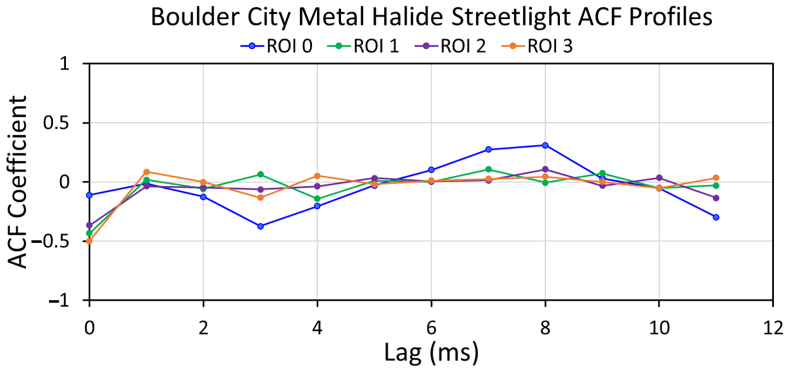
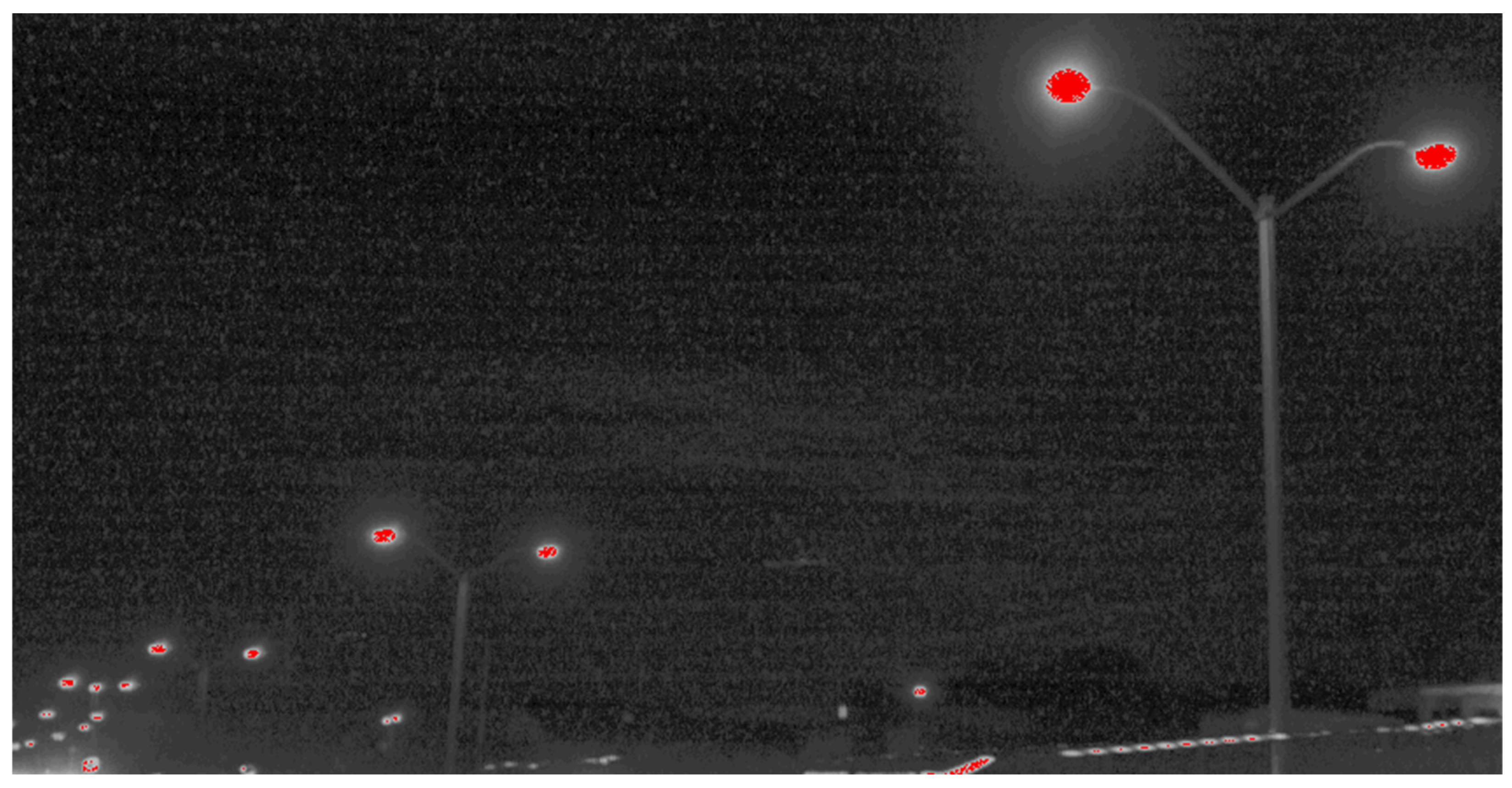
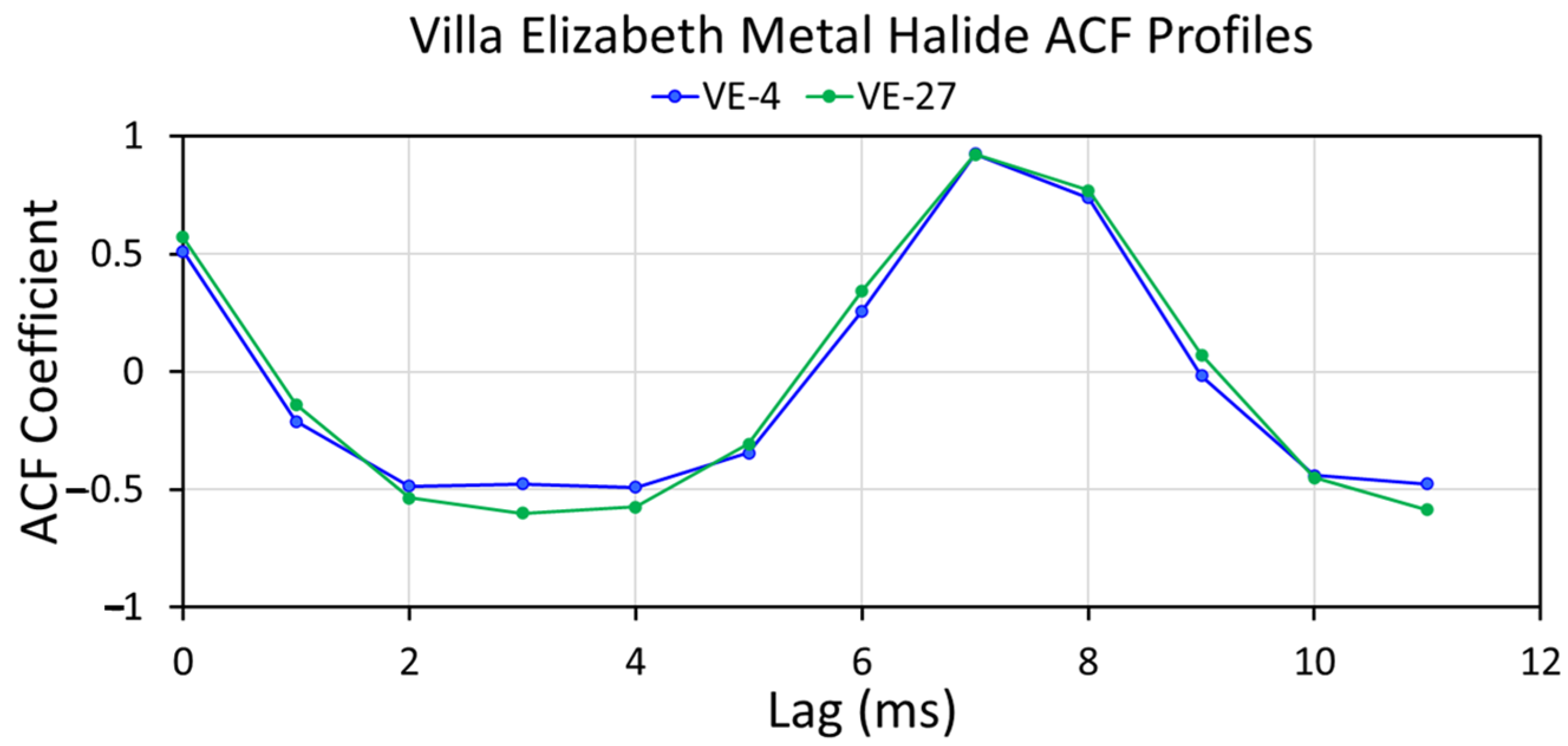
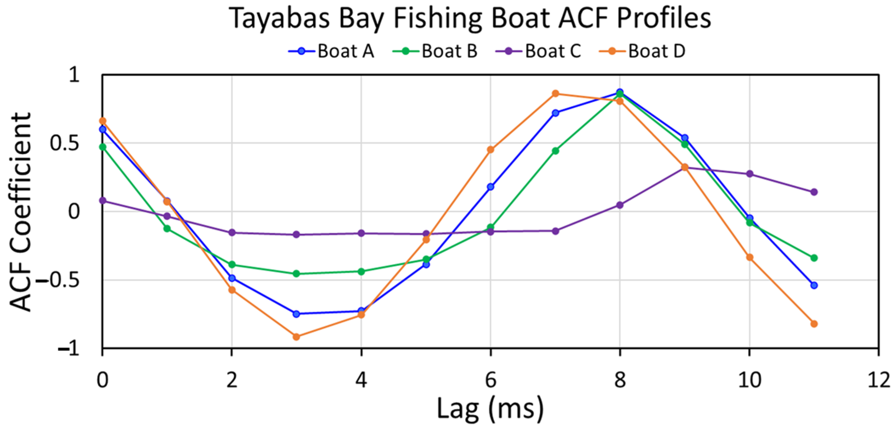
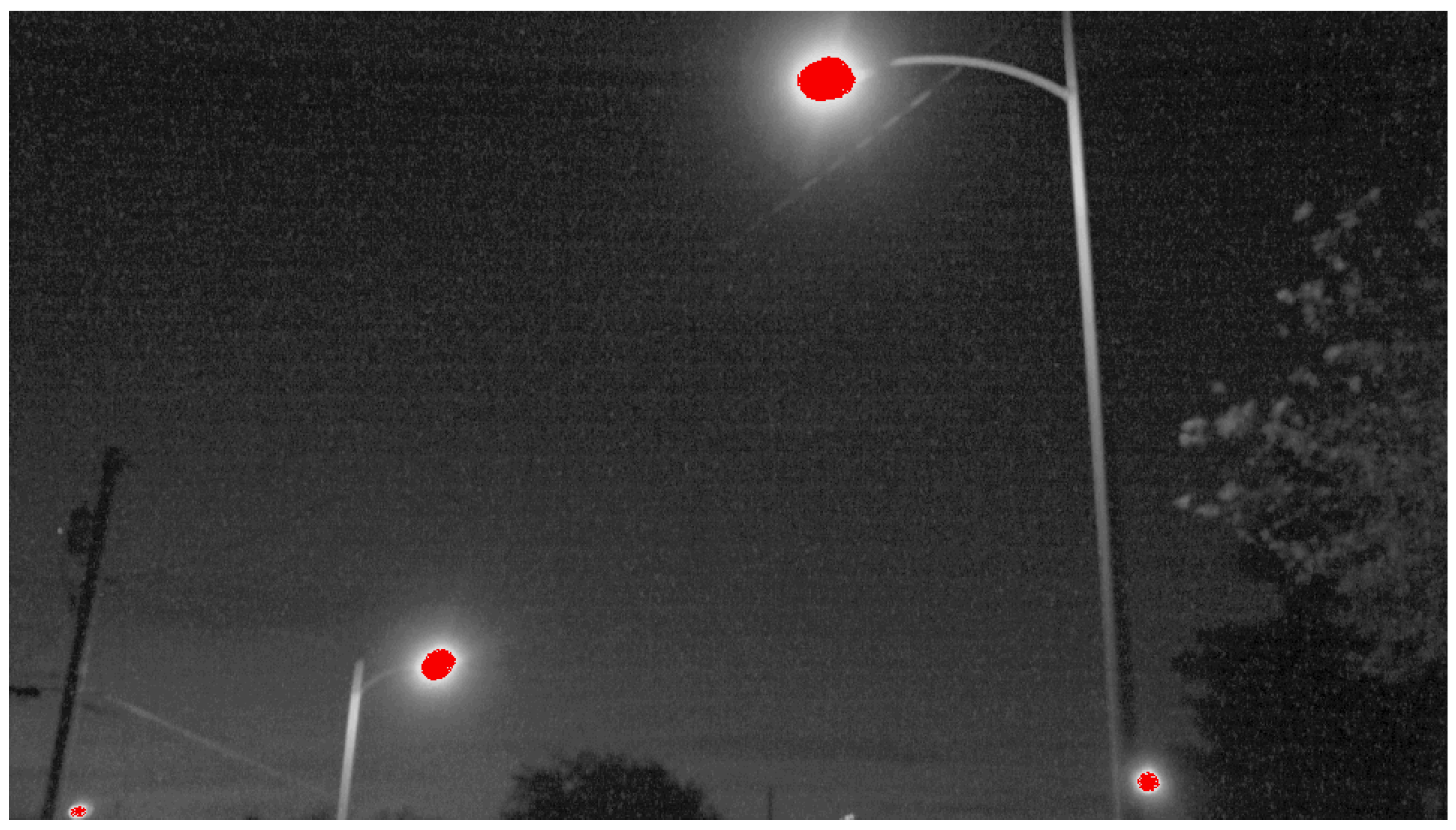
High-speed camera MP4 videos are collected in byte format, with digital numbers ranging from 0 to 255. The MP4 data are initially stored on an SD card located next to the camera battery. To analyze the flicker, the SD card must be removed, and the data must be downloaded to a computer. Dr. Mikhail Zhizhin wrote the software for the analysis of MP4 data. The software converts the color imagery to grayscale, identifies prominent lights, and draws rectangular vectors for temporal profile extraction. The presence and periodicity of lighting flicker is analyzed with an autocorrelation function (ACF) [20,43]. Starting in 2023, the high-speed camera collections were tested for the presence of saturation, which tends to dampen lighting flicker. The saturation testing is performed using the maximum brightness composite image from each MP4 by color coding pixels that have a solid color, such as red, with DN = 255. Starting in 2024, we began testing neutral density filters for the prevention of the saturation of bright luminaires.

The 2021 data were collected by measuring individual lights indoors in the EOG’s office suite at the Colorado School of Mines as part of Flickerfest, held on 28 August 2021. These collections were made with a similar Sony high-speed camera, a spectrometer, and a color still camera. The Sony camera and spectrometer were mounted on tripods for motion stabilization.

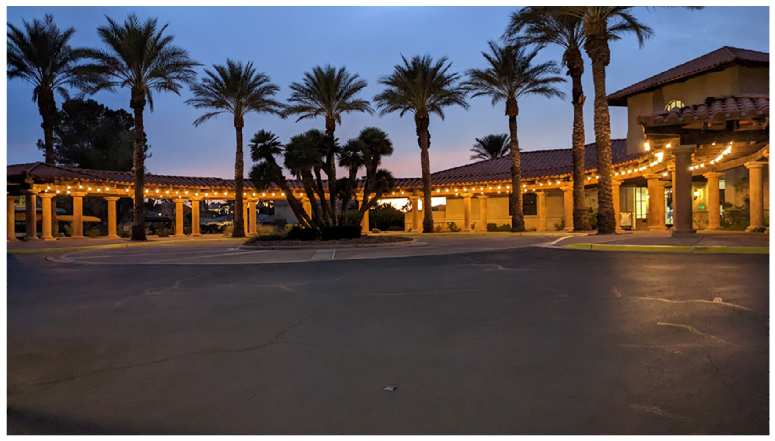
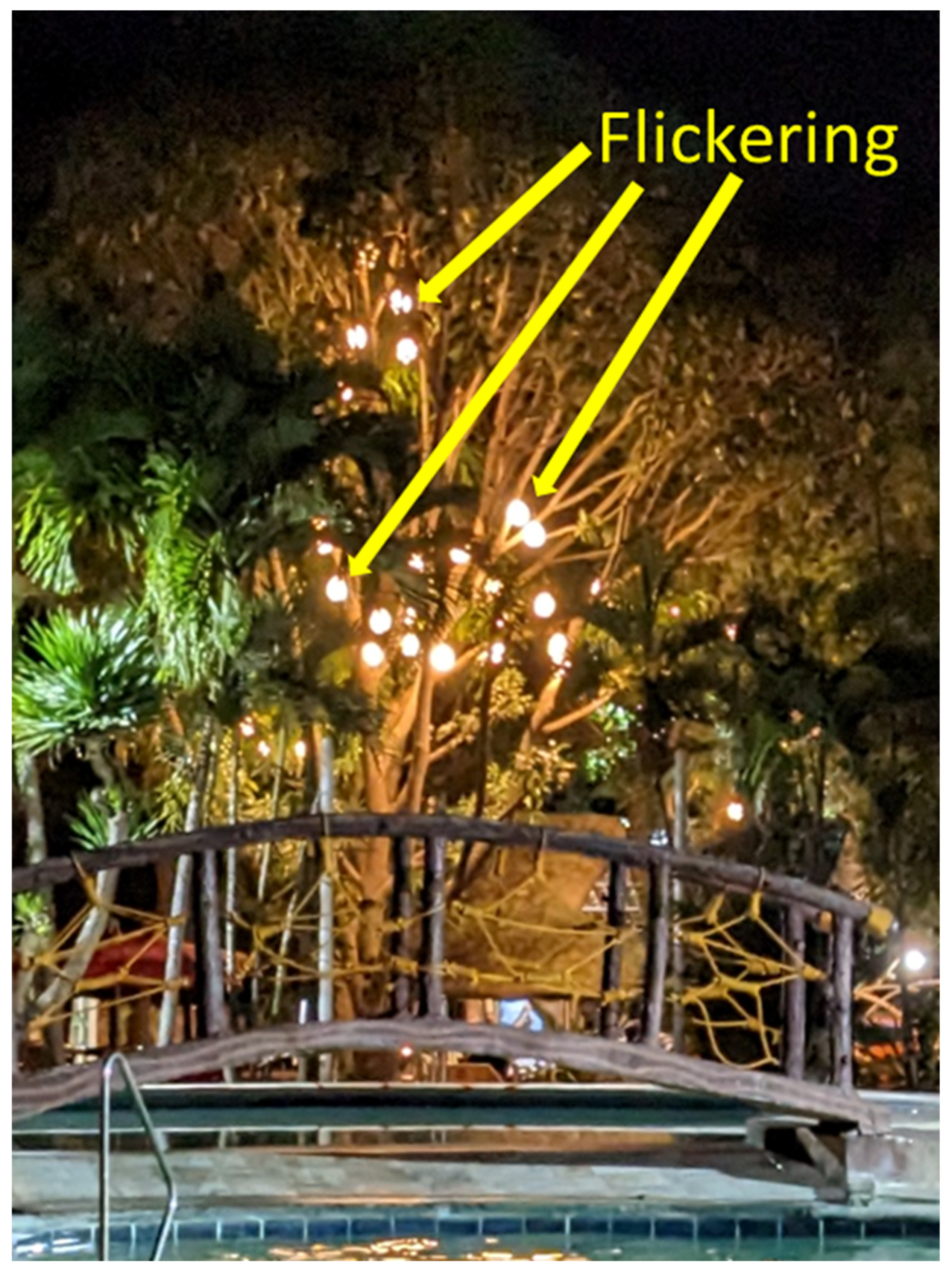
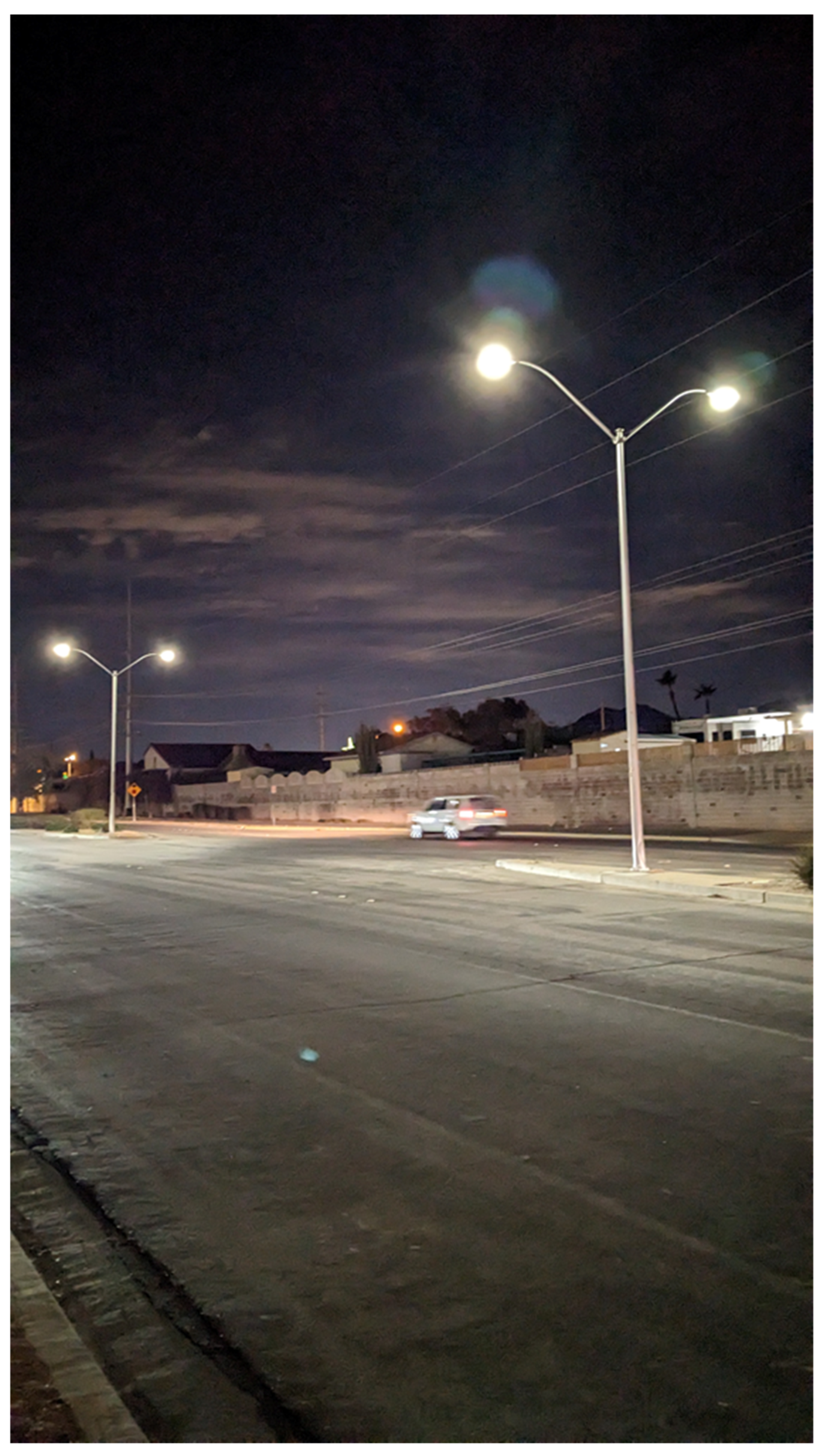
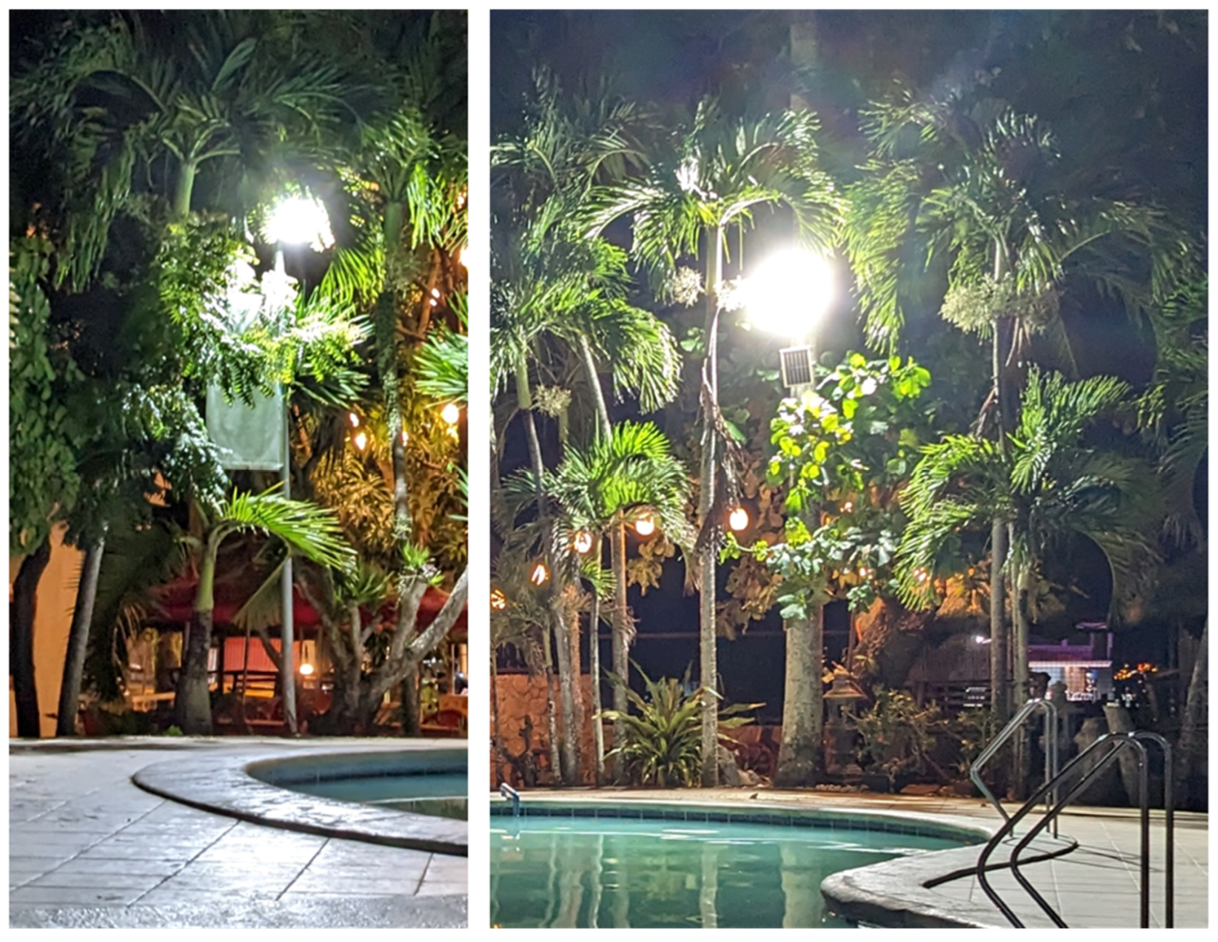
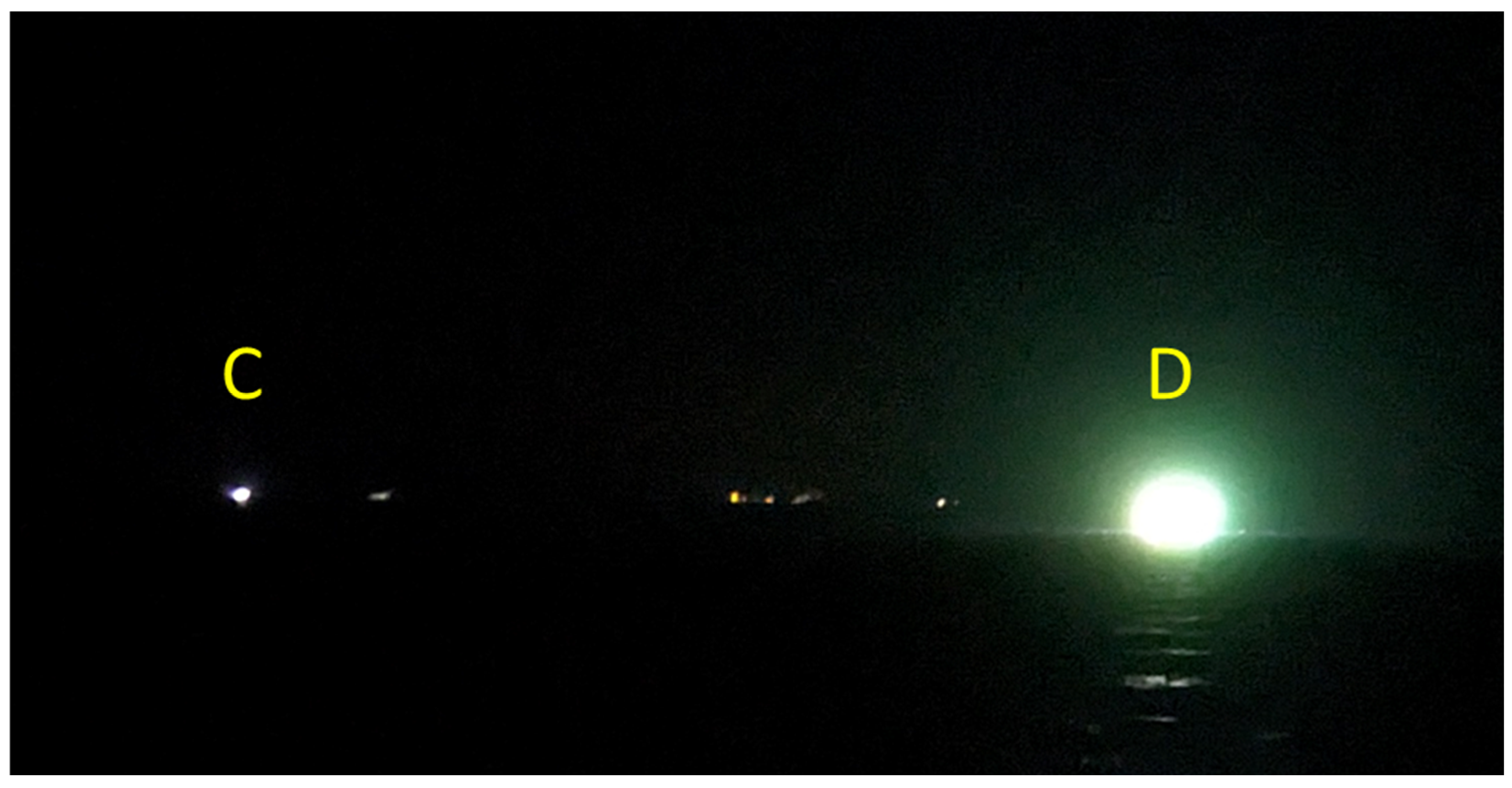
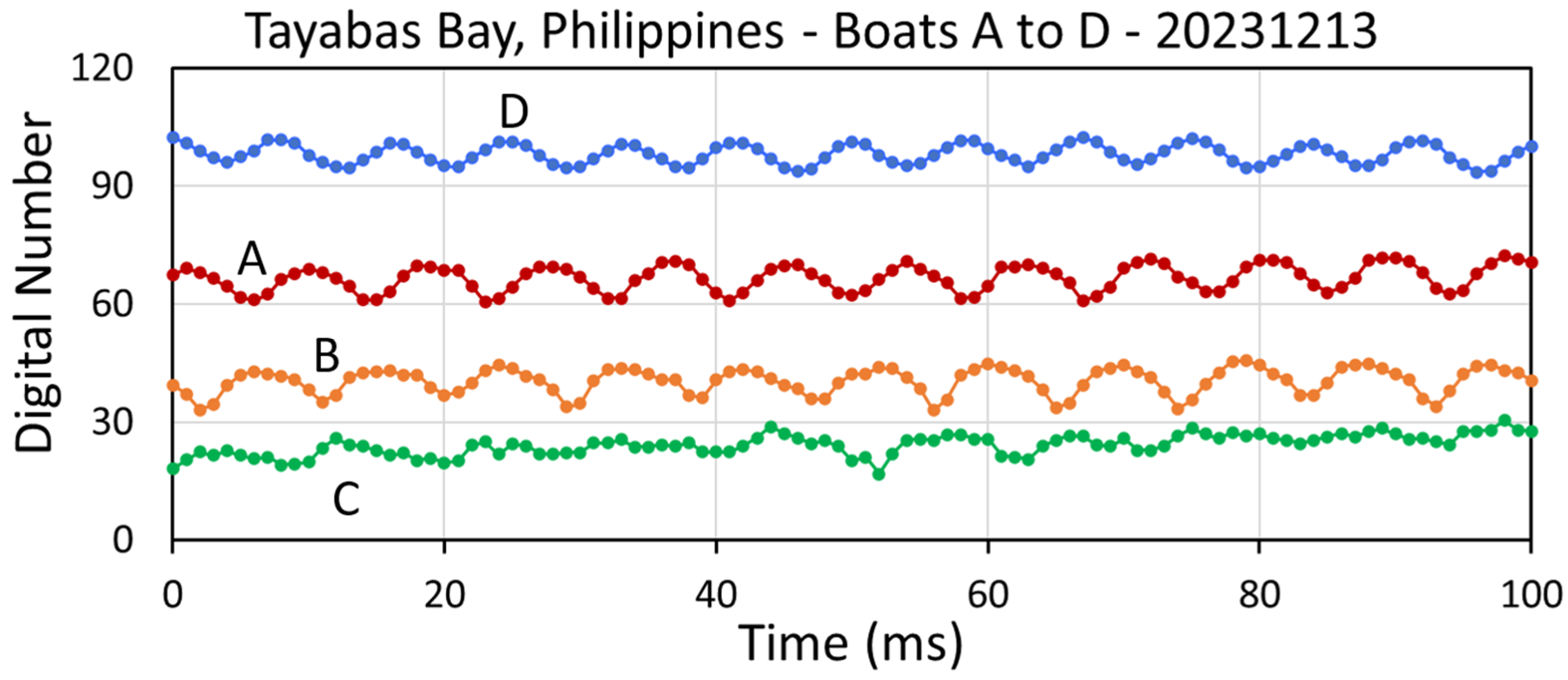
The 2023 data collection was primarily conducted on outdoor lighting, with multiple lights in each collection for the analysis of synchronization. The 2023 data collection was carried out using a high-speed camera, spectrometer, and smart phone photography at sites including the Lake Las Vegas and Heritage Park areas in Henderson, Nevada and Boulder City, Nevada. High-speed camera data were also collected at onshore and offshore sites in the Philippines. The onshore site in the Philippines was the Villa Elizabeth Beach Resort in Lucena, Quezon Province. Offshore high-speed camera data were collected for lit fishing boats in the Tayabas Bay observed at night from a passenger ferry enroute between the ports of Lucena and Balanacan.

In 2024, collections were made on or near the campus of the Asian Institute of Technology (AIT), north of Bangkok, Thailand, and at three of the previously measured sites in Henderson, Nevada. The 2024 Sony camera data collection investigated the elimination of saturation using neutral density filters. This includes collections with and without the Sony camera’s built-in three stop (12.5% transmissivity) ND filter and the camera’s automatic ND setting. In addition, at Heritage Park sport fields in Henderson, Nevada, the 2024 Sony camera collections also include two external ND filters—one with 1.56% transmissivity (6 stop) and the other with 0.016% transmissivity (16 stop).

The 2024 spectrometer collections also examined the detection of flicker and spectral changes associated with the cooling of lights during the trough phase of flickering. This data collection was conducted using a 3.8 millisecond integration time, the shortest that is possible with the USB-4000. Collection sites included an LED spotlight Thammasat University entry sign along Highway 1, north of Bangkok, and metal halide luminaire clusters on tall poles at the Heritage Park sport field in Henderson, Nevada.

4. Results

4.1. LED Luminaires

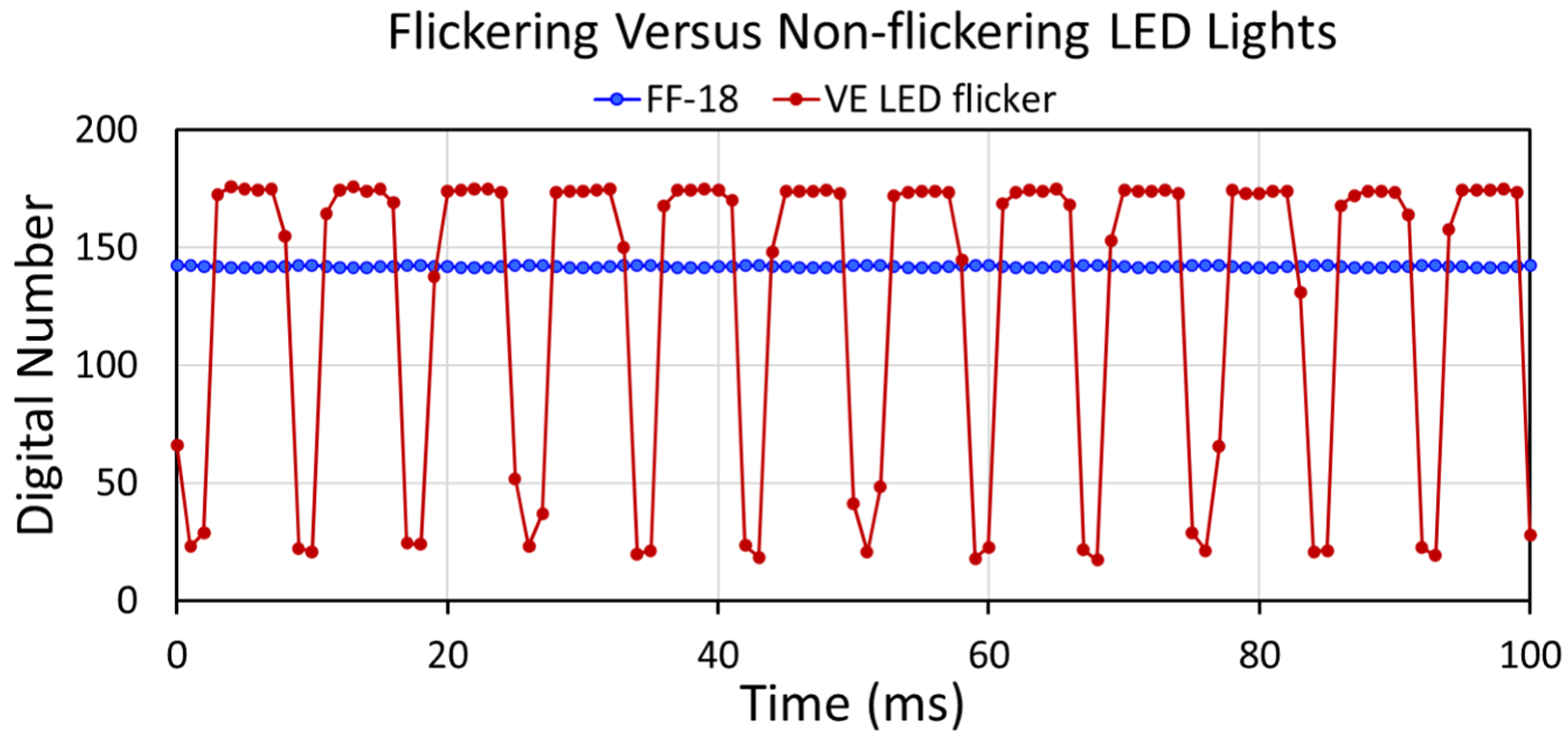
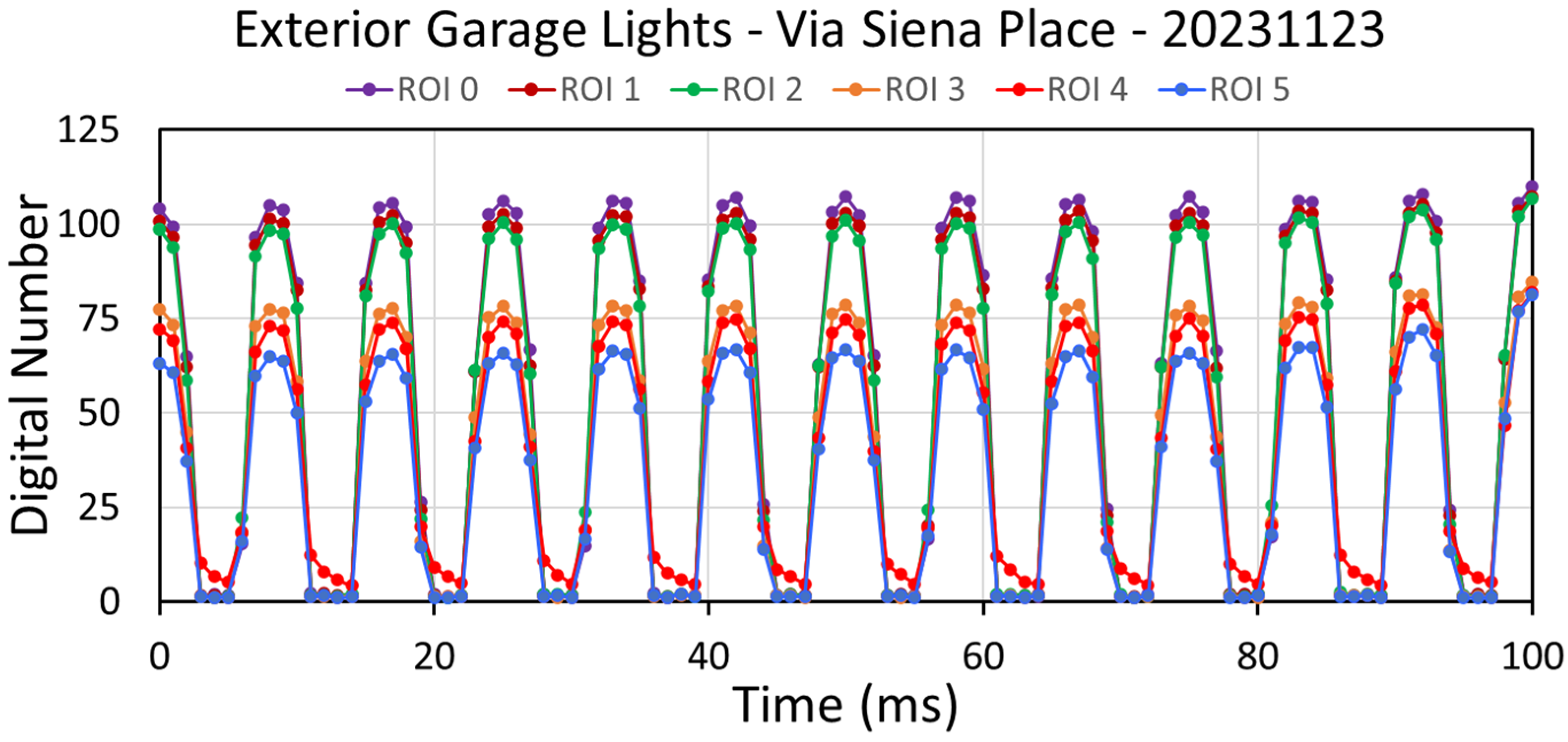
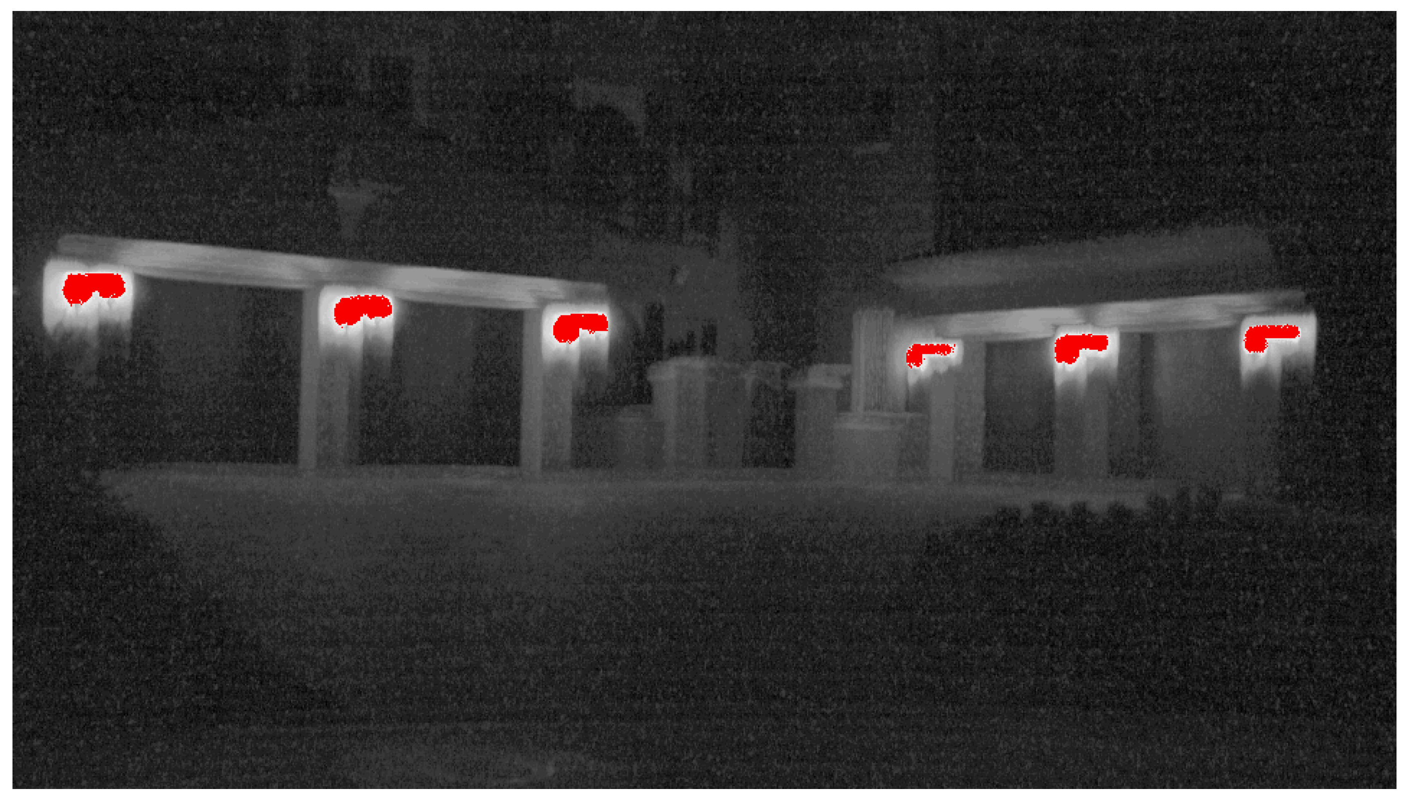
LED luminaires create light through electroluminescence. Photons are discharged when excited electrons drop to a lower-energy orbital shell. LED luminaires come in both flickering and non-flickering varieties (Figure 1). Non-flickering LED luminaires were measured during Flickerfest in 2021 [20] (Figure A1, Figure A2, Figure A3 and Figure A4), in Boulder City, Nevada in 2023, and at the Asian Institute of Technology in 2024. Flickering LED lights were measured at sites in Henderson, Nevada; Lucena, Philippines; and near AIT in Thailand. Results from specific LED collections are presented in Appendix A.1 (Figure A1, Figure A2, Figure A3, Figure A4, Figure A5, Figure A6, Figure A7, Figure A8, Figure A9, Figure A10, Figure A11, Figure A12, Figure A13, Figure A14, Figure A15, Figure A16, Figure A17, Figure A18, Figure A19, Figure A20, Figure A21, Figure A22, Figure A23, Figure A24, Figure A25 and Figure A26).

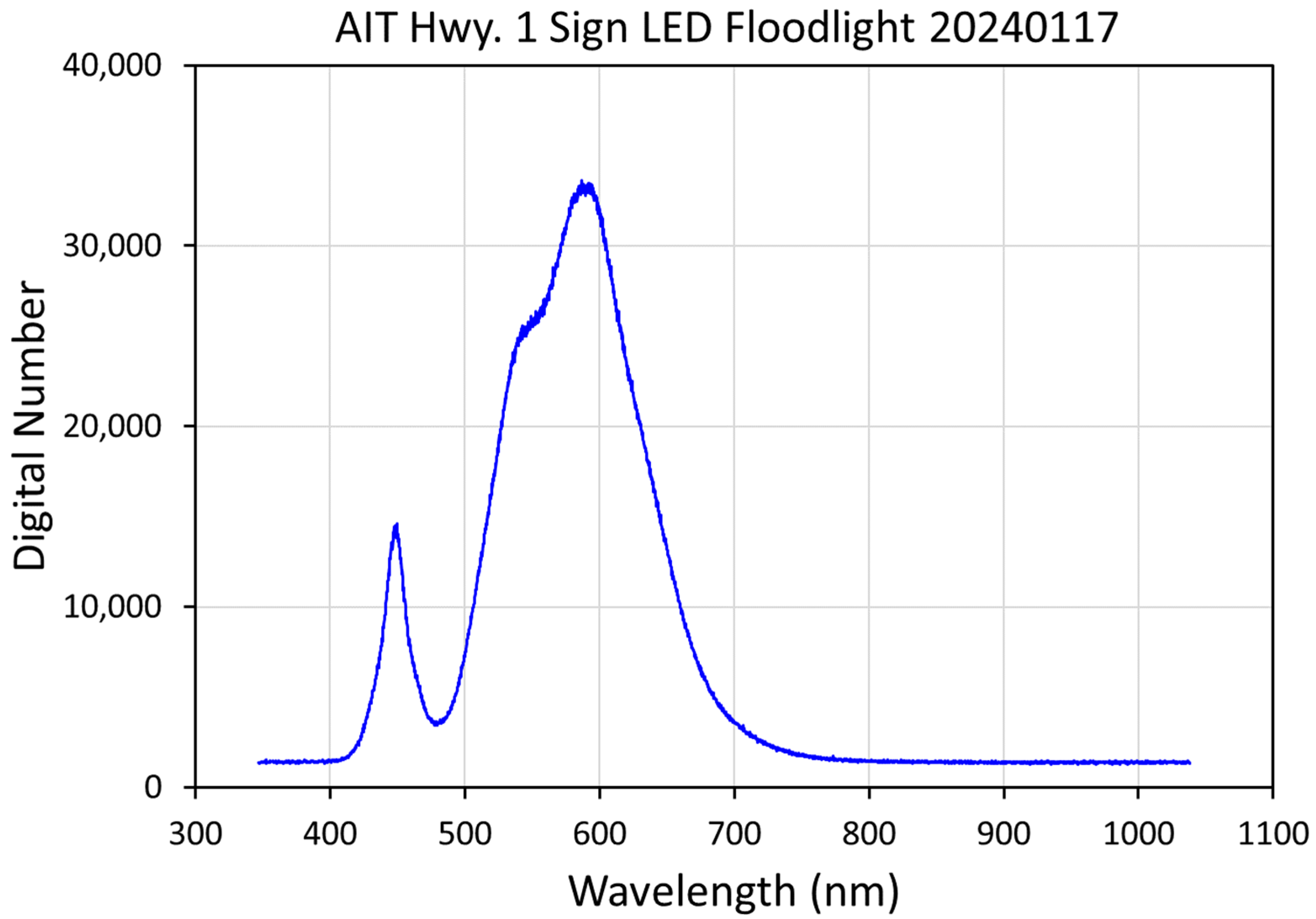
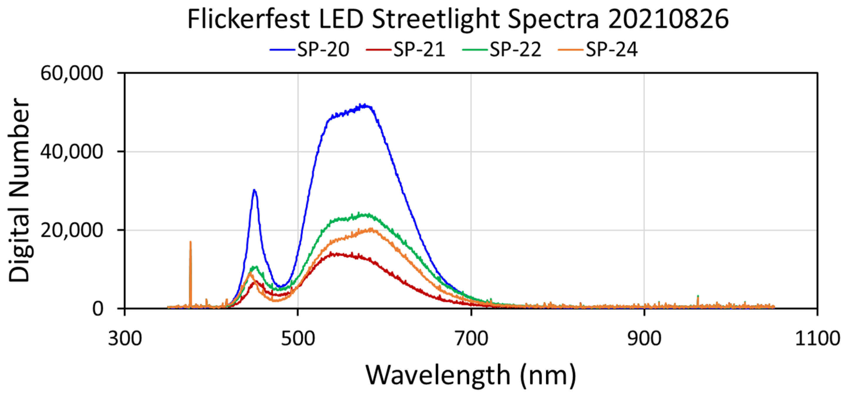
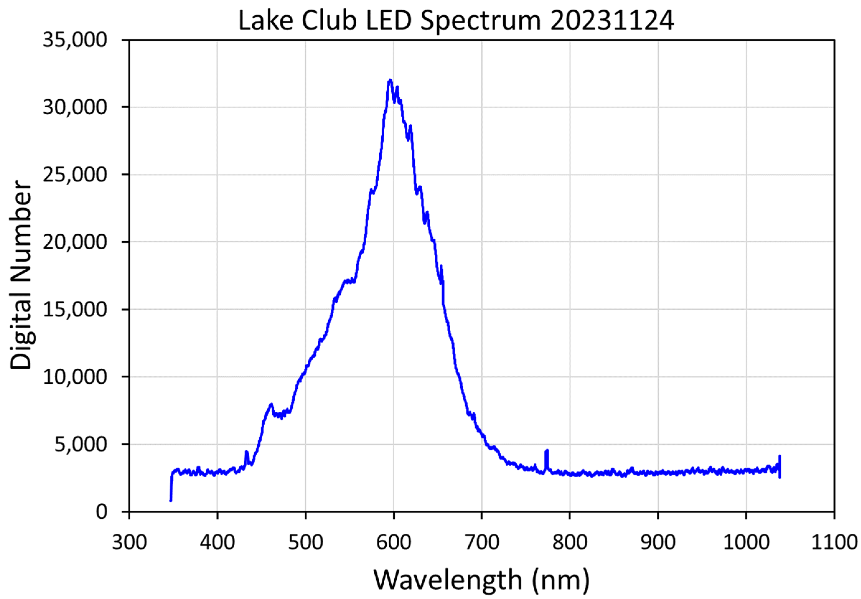
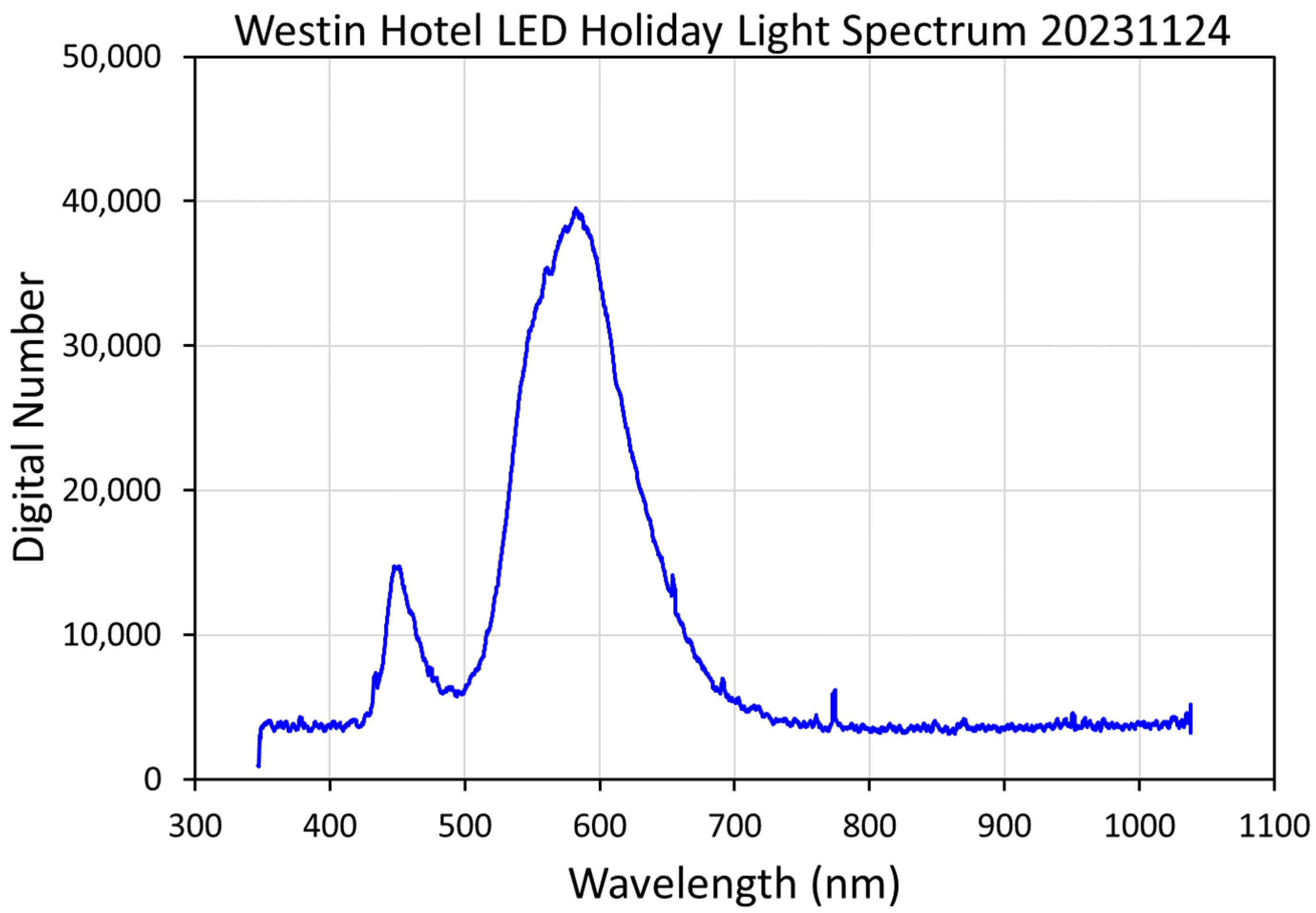
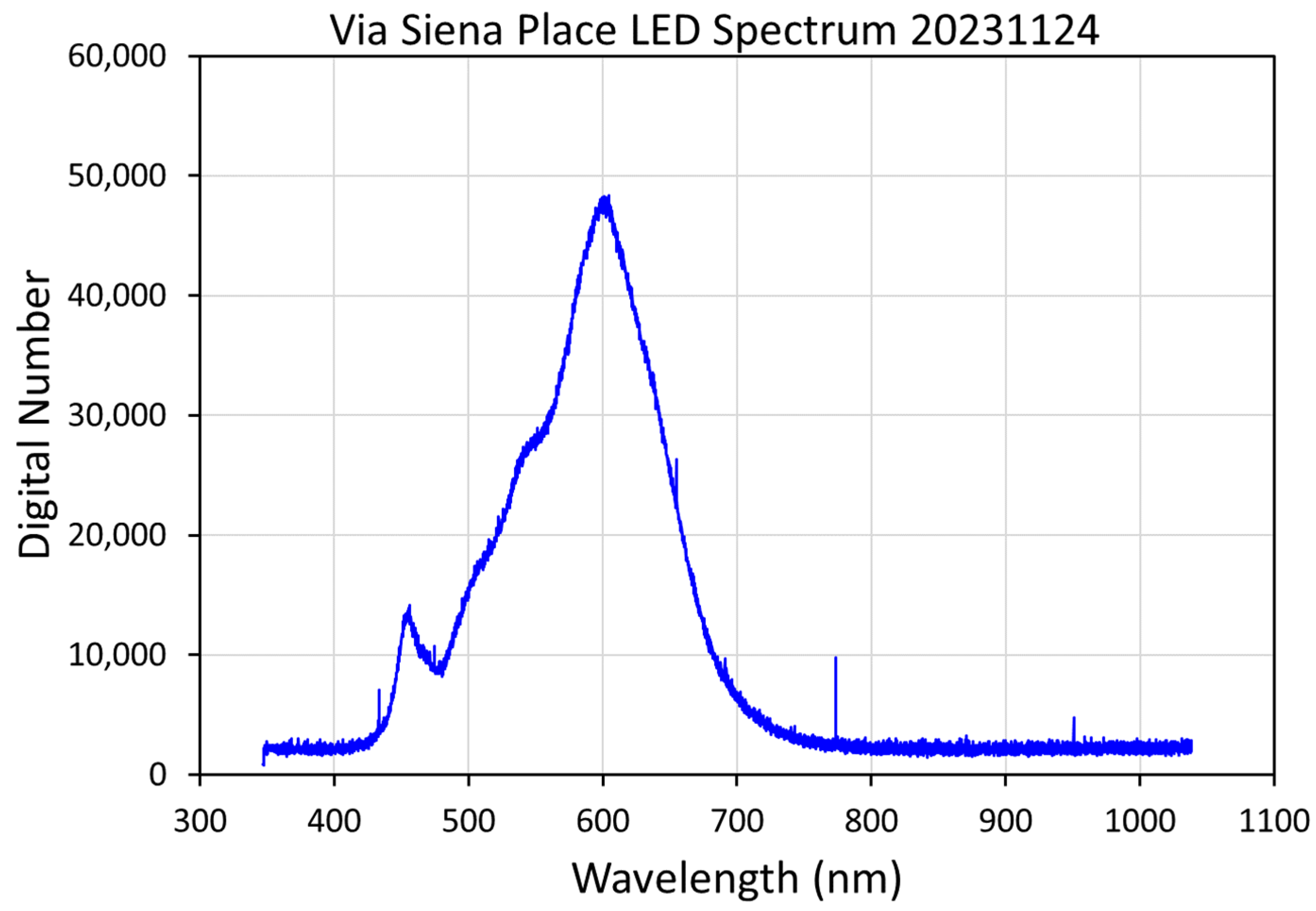
LED luminaires are distinct from other types of lighting in the following aspects: (1) they operate at near-ambient temperatures; (2) their radiant output is concentrated in one or more broad lobe-like features in the visible range, such that LEDs with blue and orange lobes have a phosphorus coating to absorb blue light and re-emit at longer visible wavelengths (Figure 2); (3) they have relatively few elemental line emissions [44]; and (4) they have very low light output beyond 700 nm [44]. It should be noted that the spectra of flickering and non-flickering LEDs look quite similar.

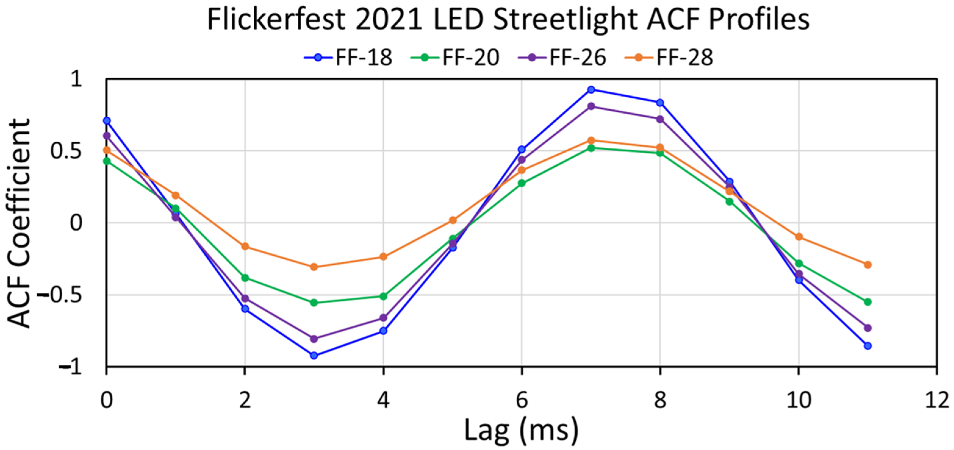
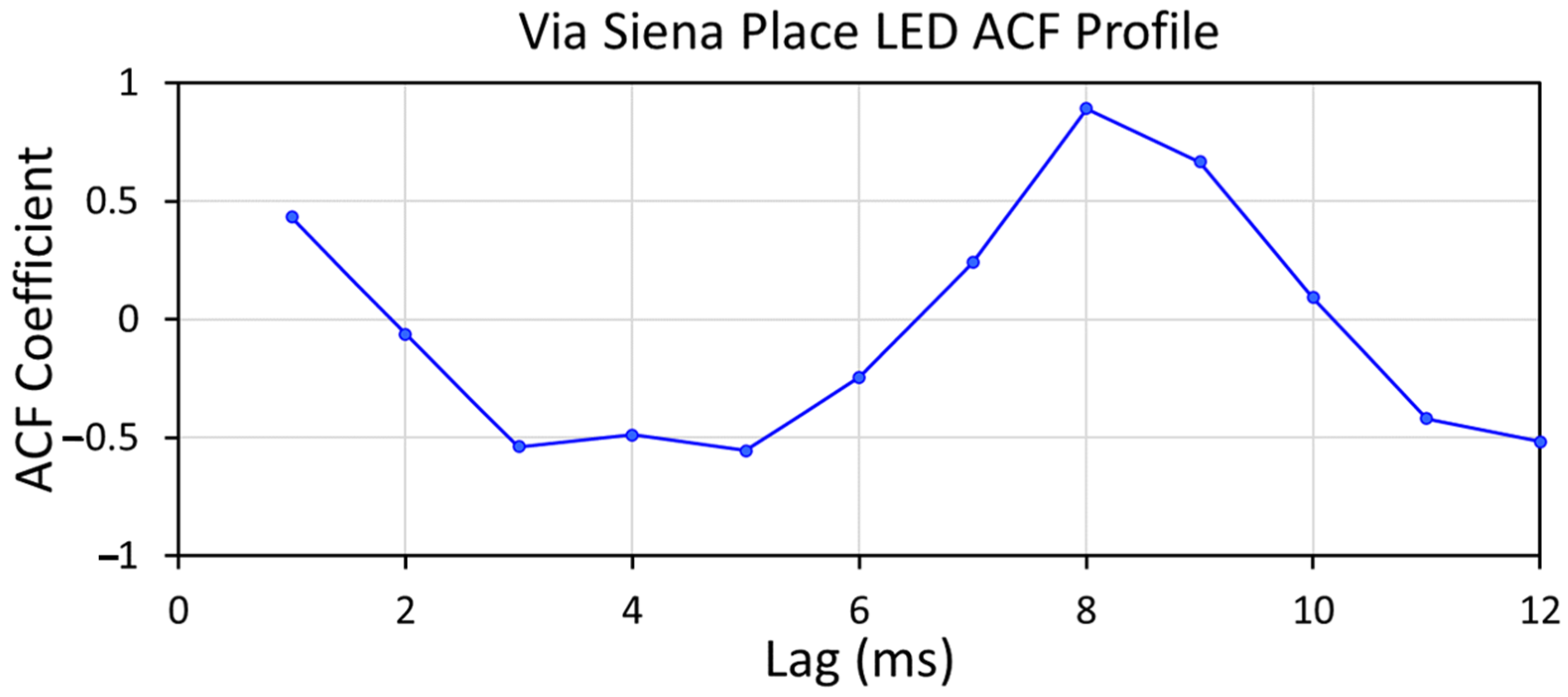
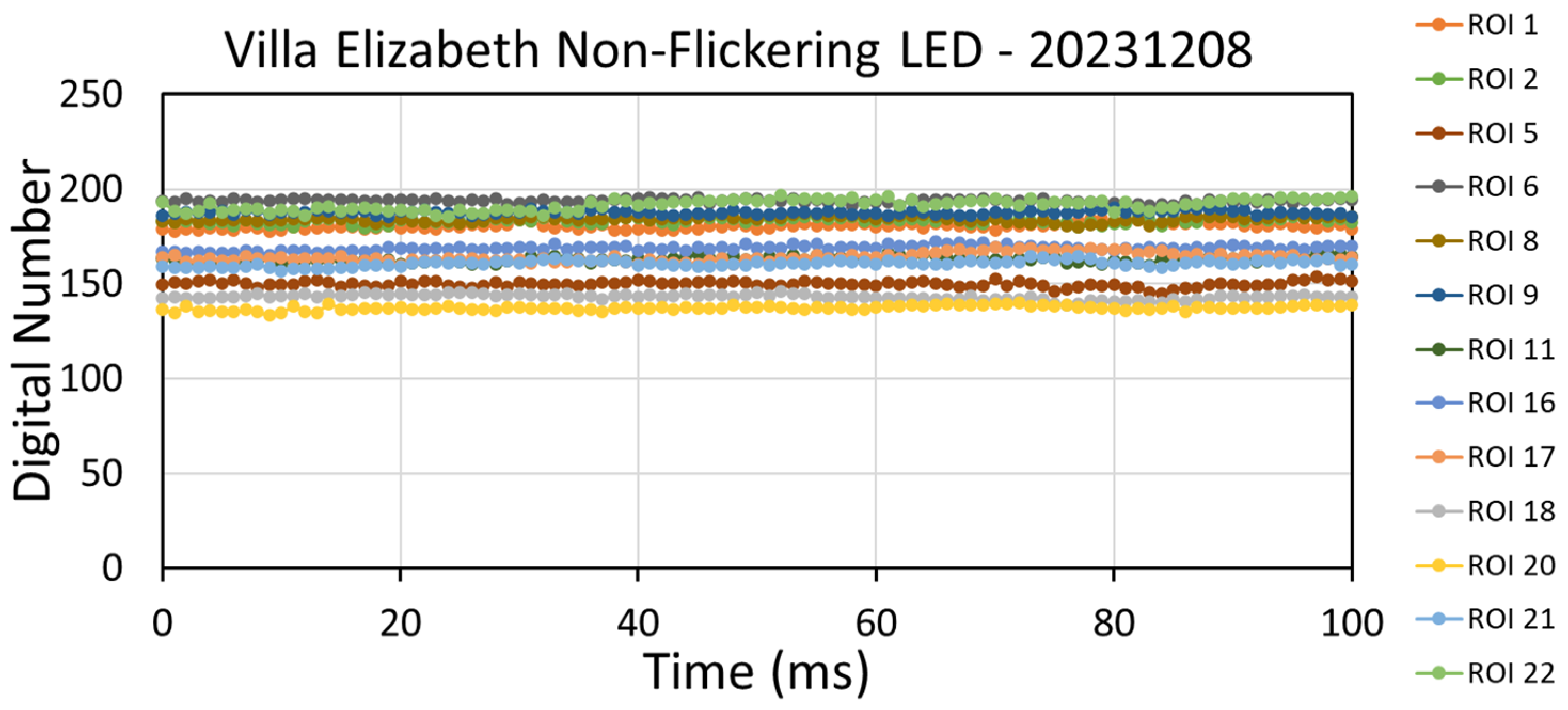
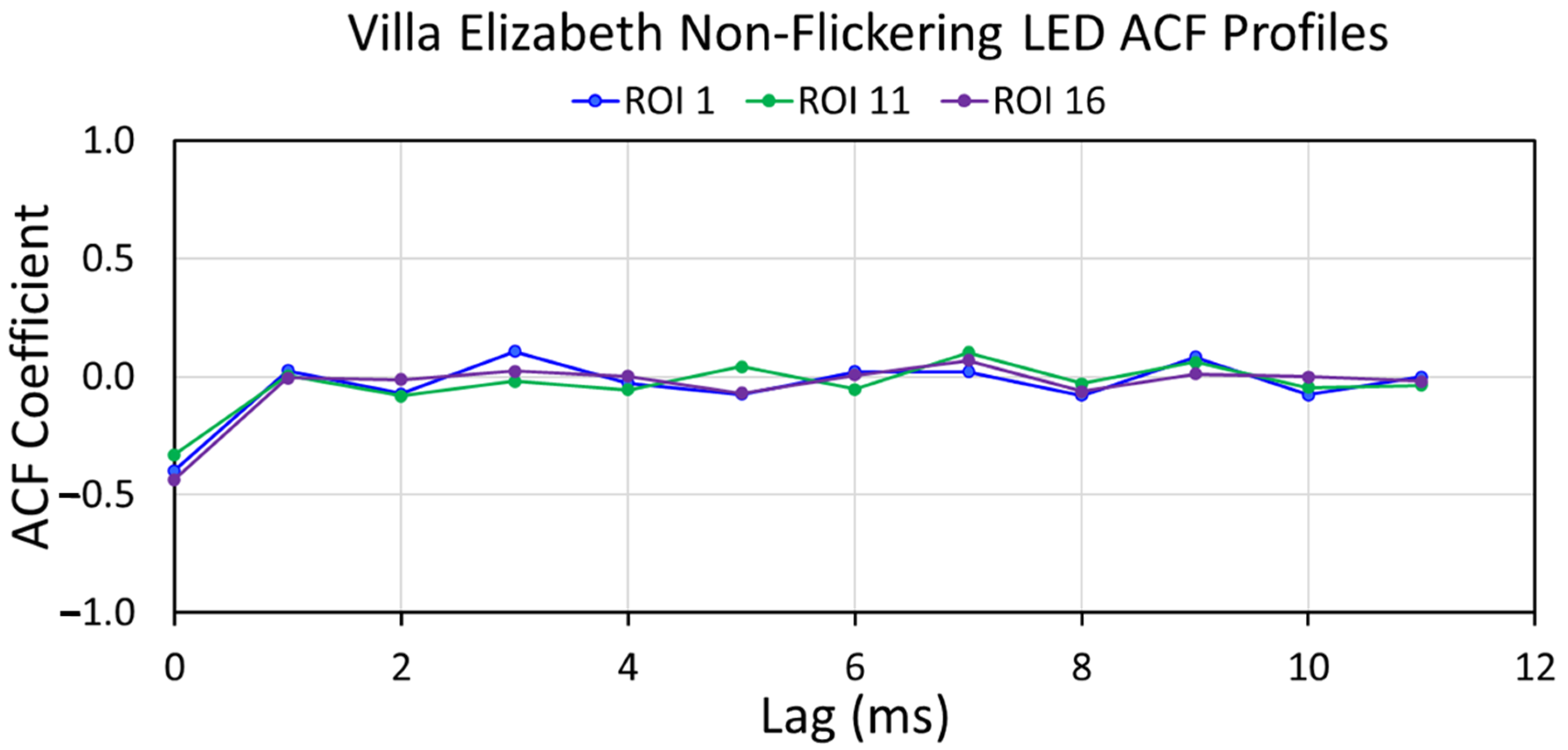
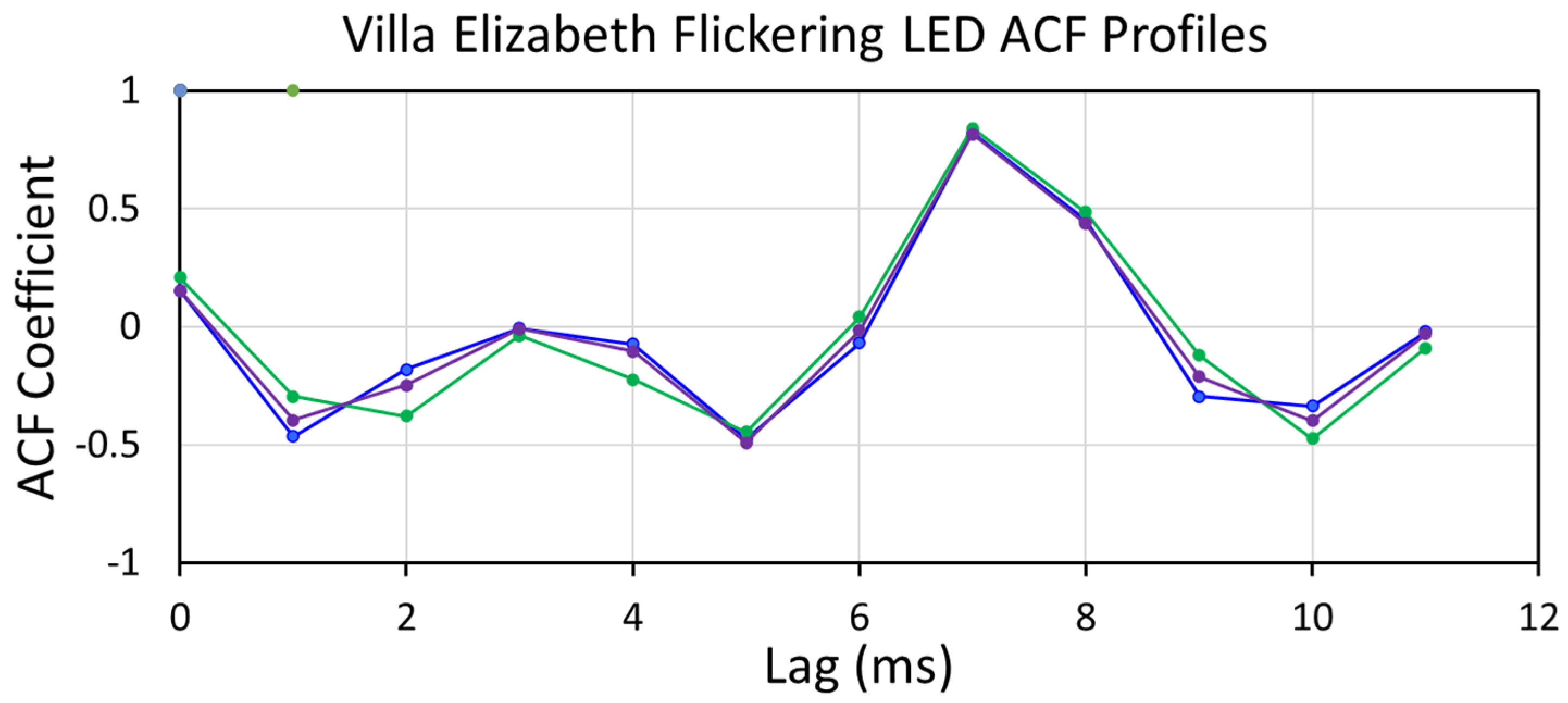
Non-flickering LED luminaires have built-in electronic drivers [45] that smooth the alternating current so thoroughly that the flicker can appear absent. This leads to extremely low percent flicker values, but the presence of flicker may still be detected in their autocorrelation function (ACF) profiles (Figure A4). Flickering LEDs have extremely high percent flicker values, as compared to other light sources.

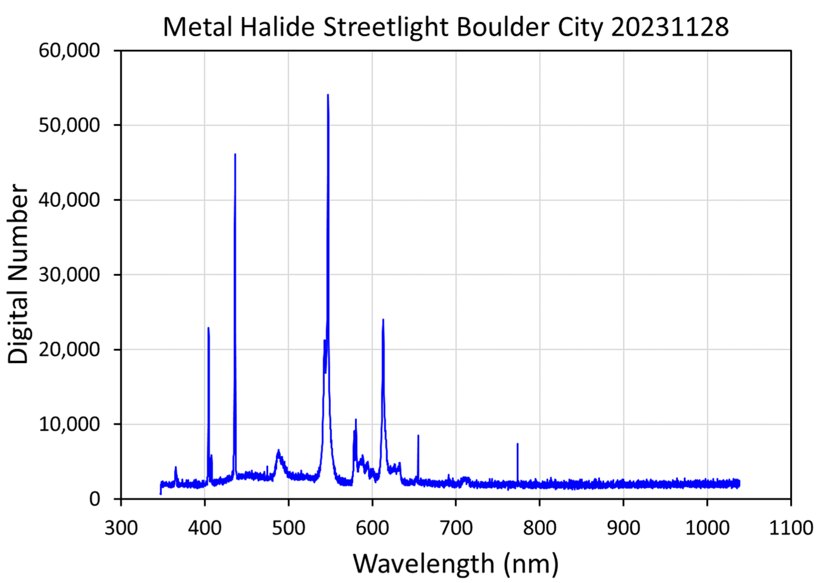
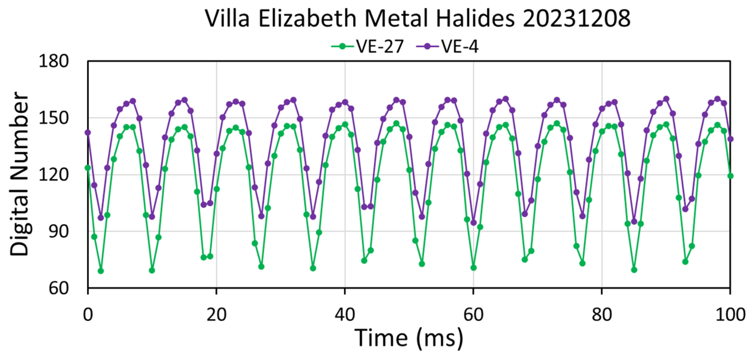
4.2. Metal Halide Luminaires

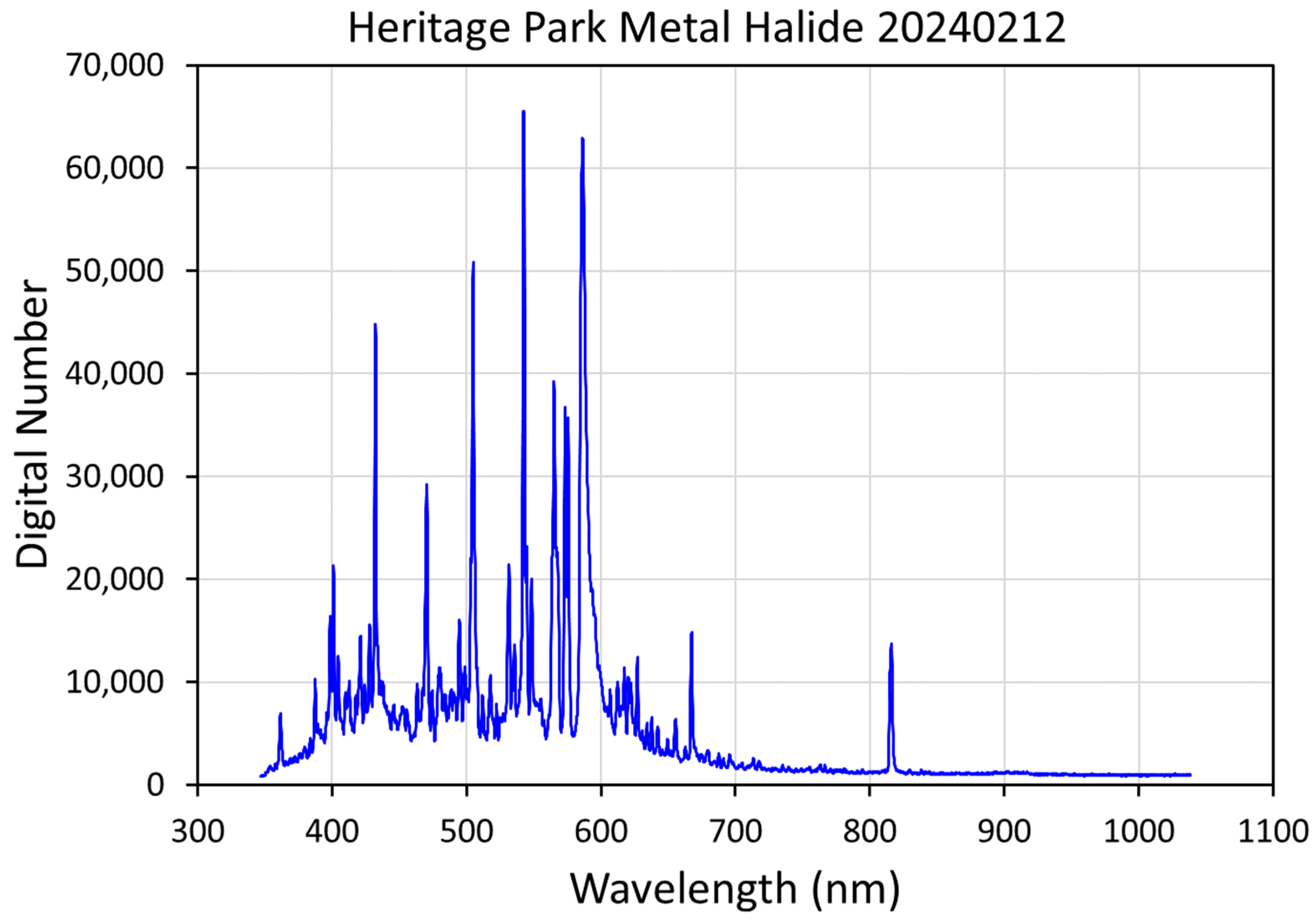
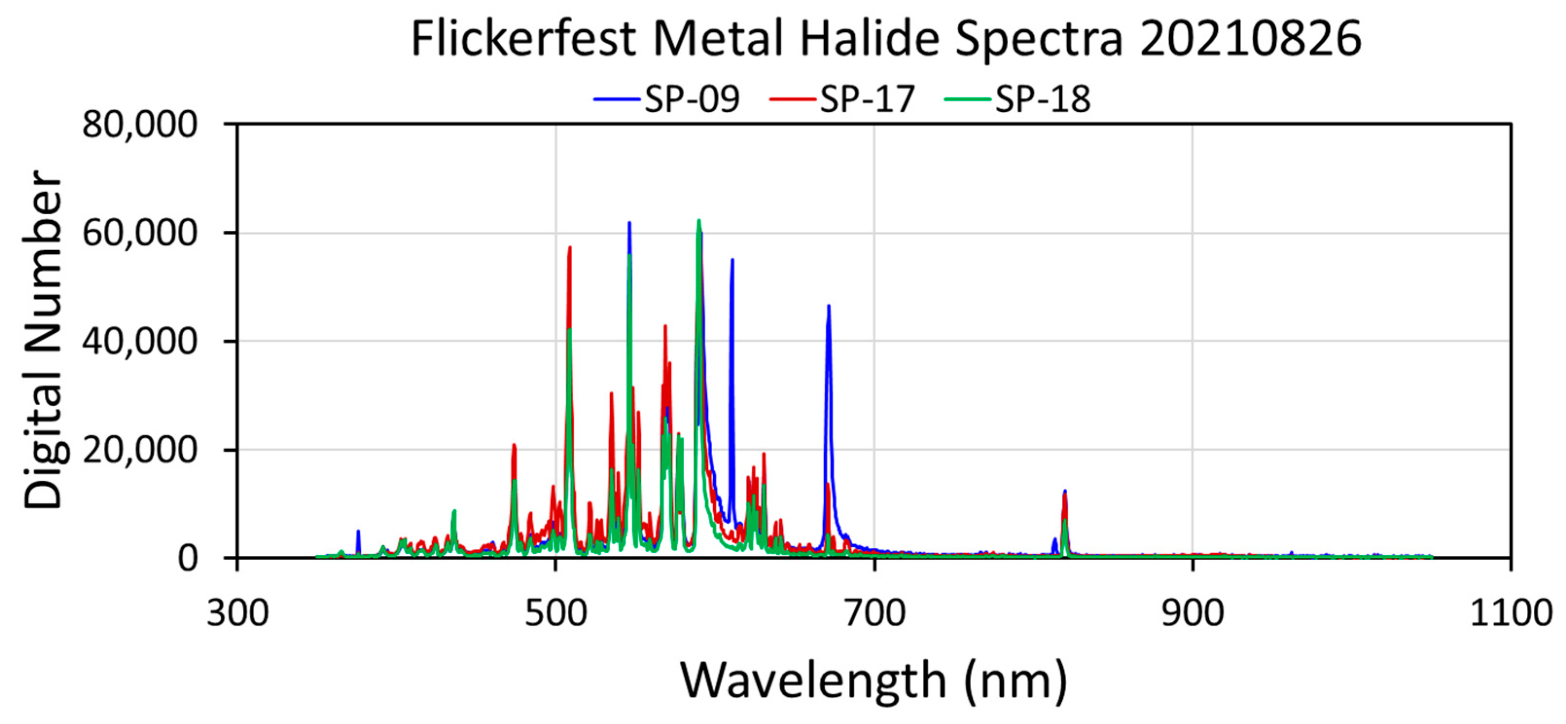
Metal halide luminaires belong to the high-intensity discharge (HID) class of lights, along with sodium lights. Metal halides produce light with high-temperature plasma inside a sealed glass enclosure [46]. Photons are produced when excited electrons in the plasma drop to lower-energy orbital shells. The compositions of the plasmas are variable mixtures of mercury, argon, xenon, and metal halides, (e.g., sodium iodide and scandium iodide). Manufacturers manipulate the plasma constituents to achieve various color profiles and color temperatures. Thus, metal halide spectra are highly variable depending on the constituents used in the glass enclosures. 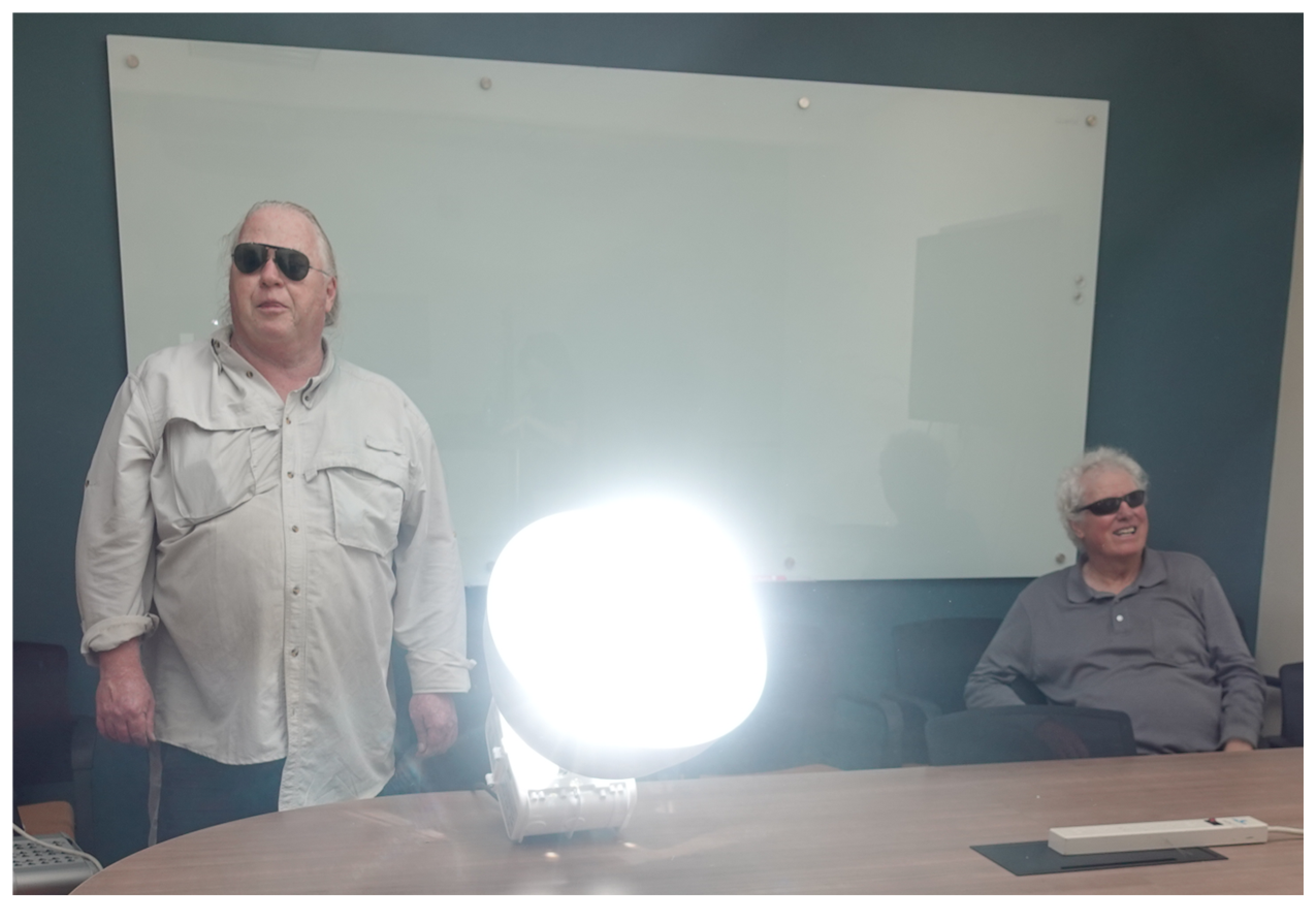Figure 3 shows the spectrum of a tall-pole-mounted cluster of metal halide luminaires at the Heritage Park sport fields in Henderson, Nevada.

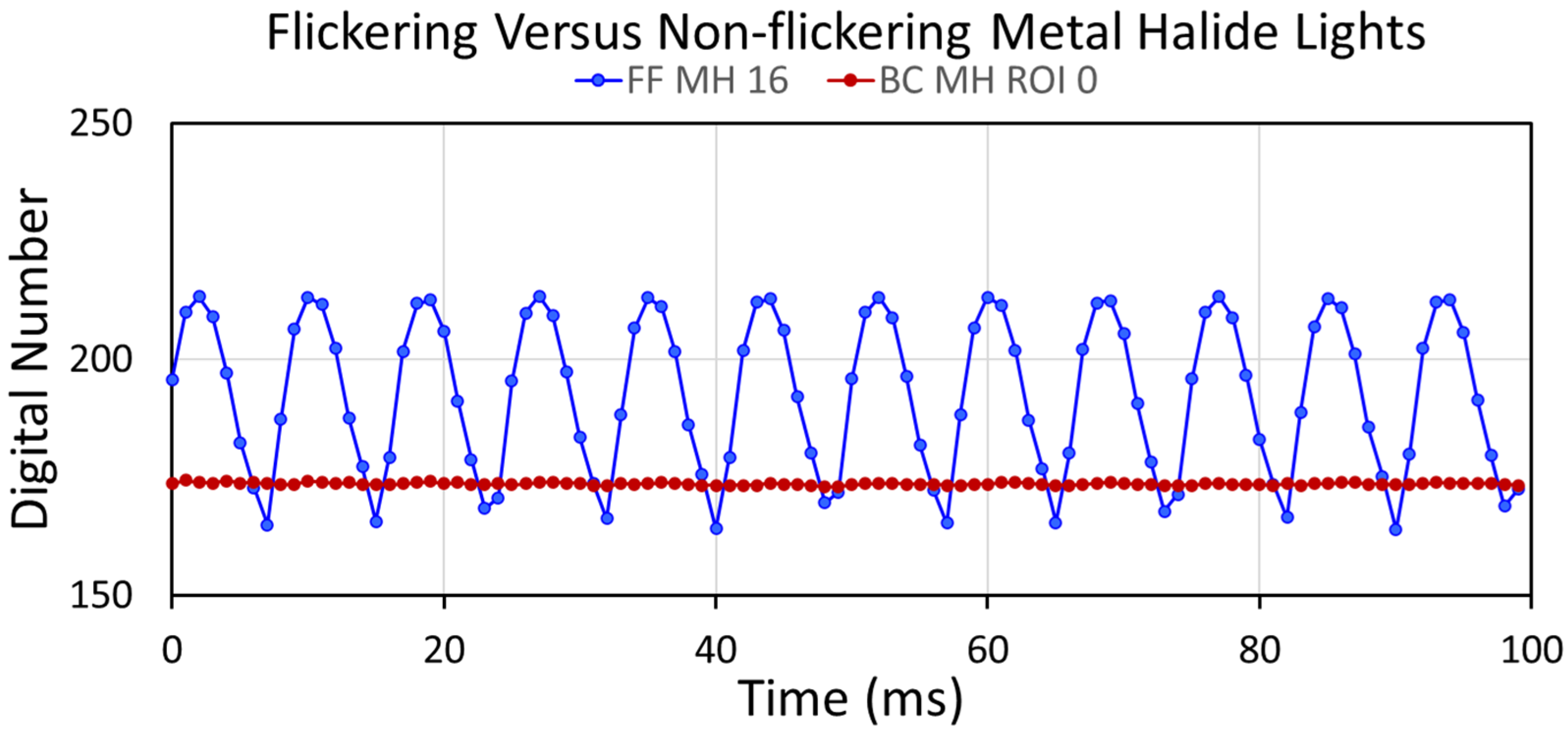
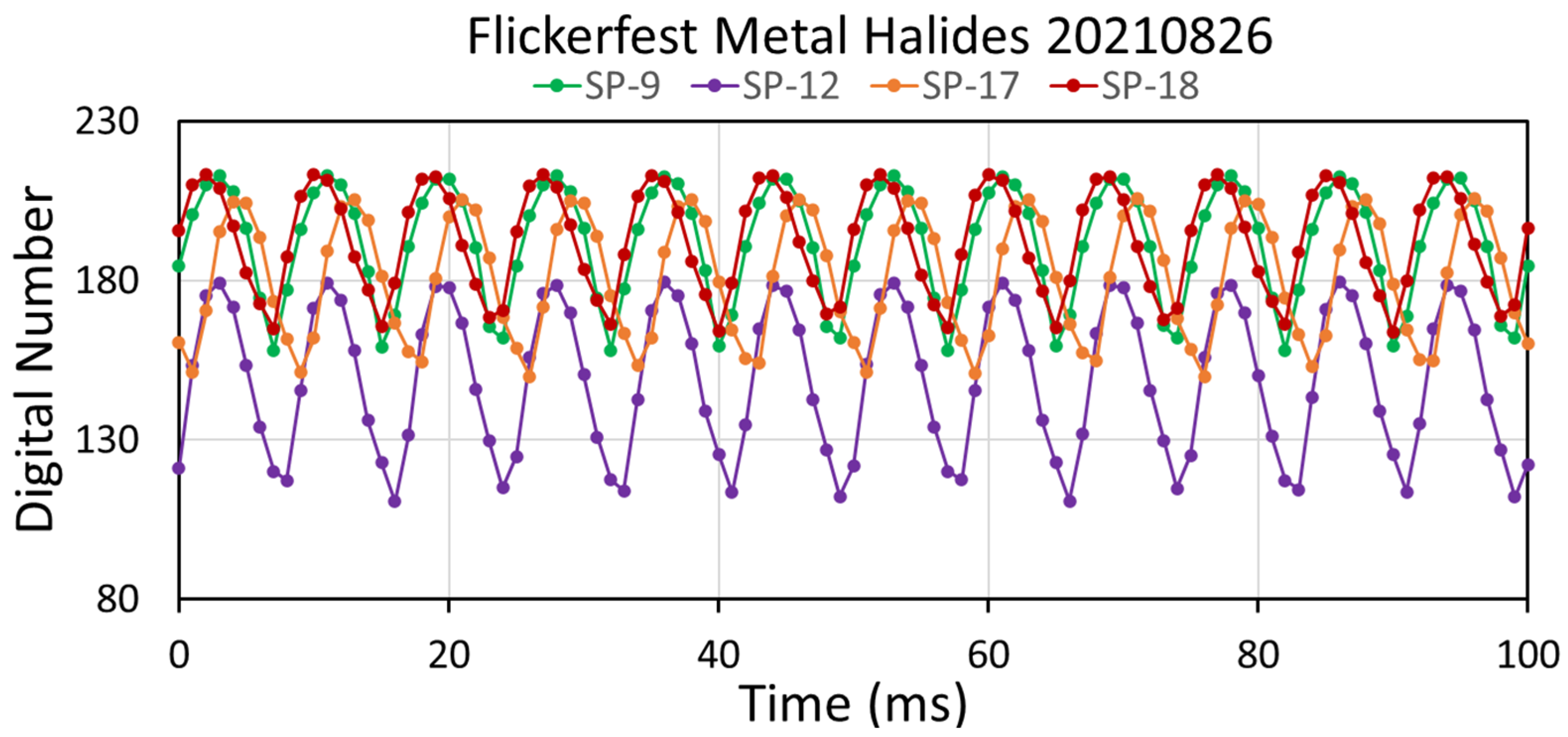
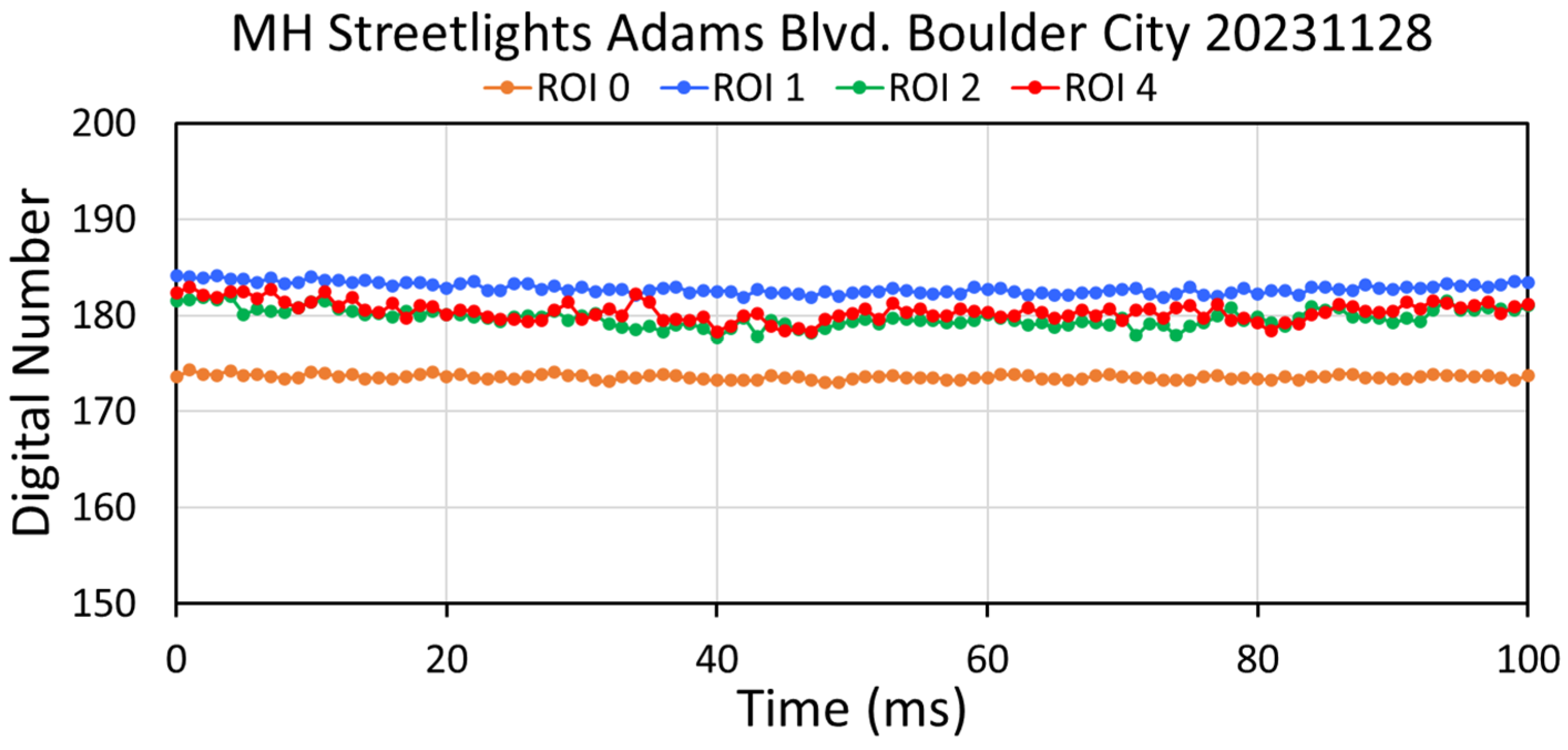
As with LED, metal halide lights can be flickering or non-flickering (Figure 4). 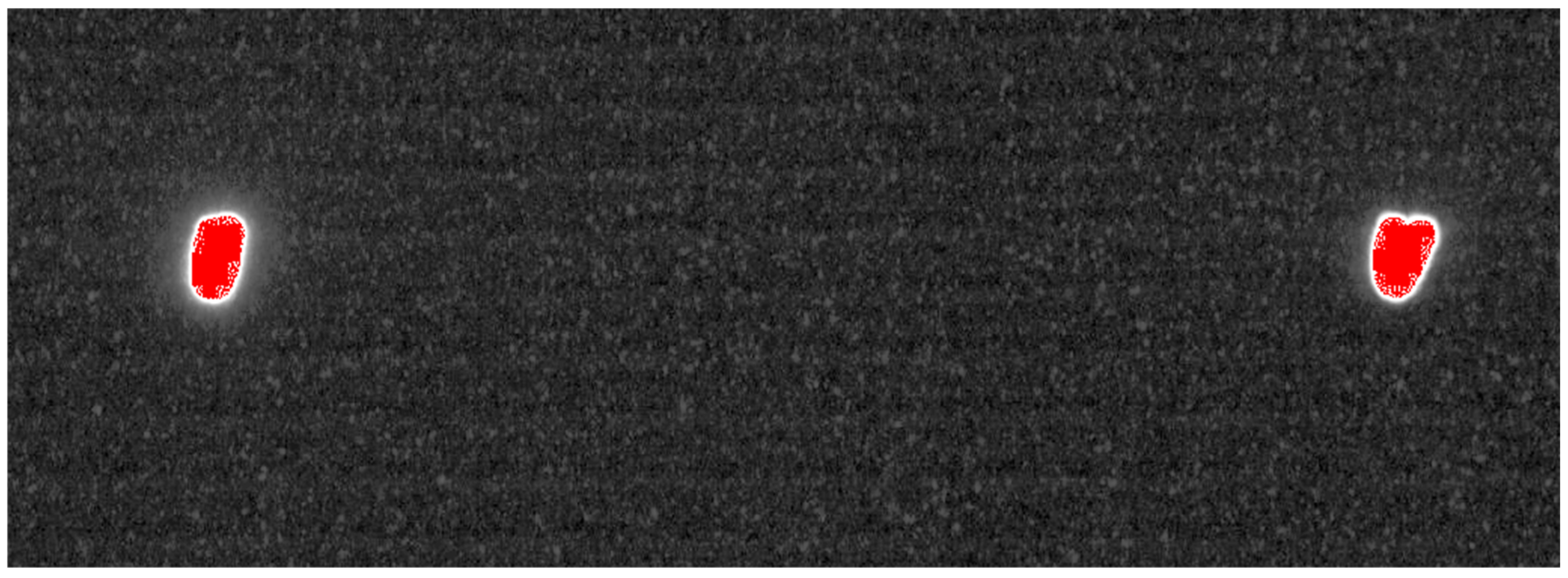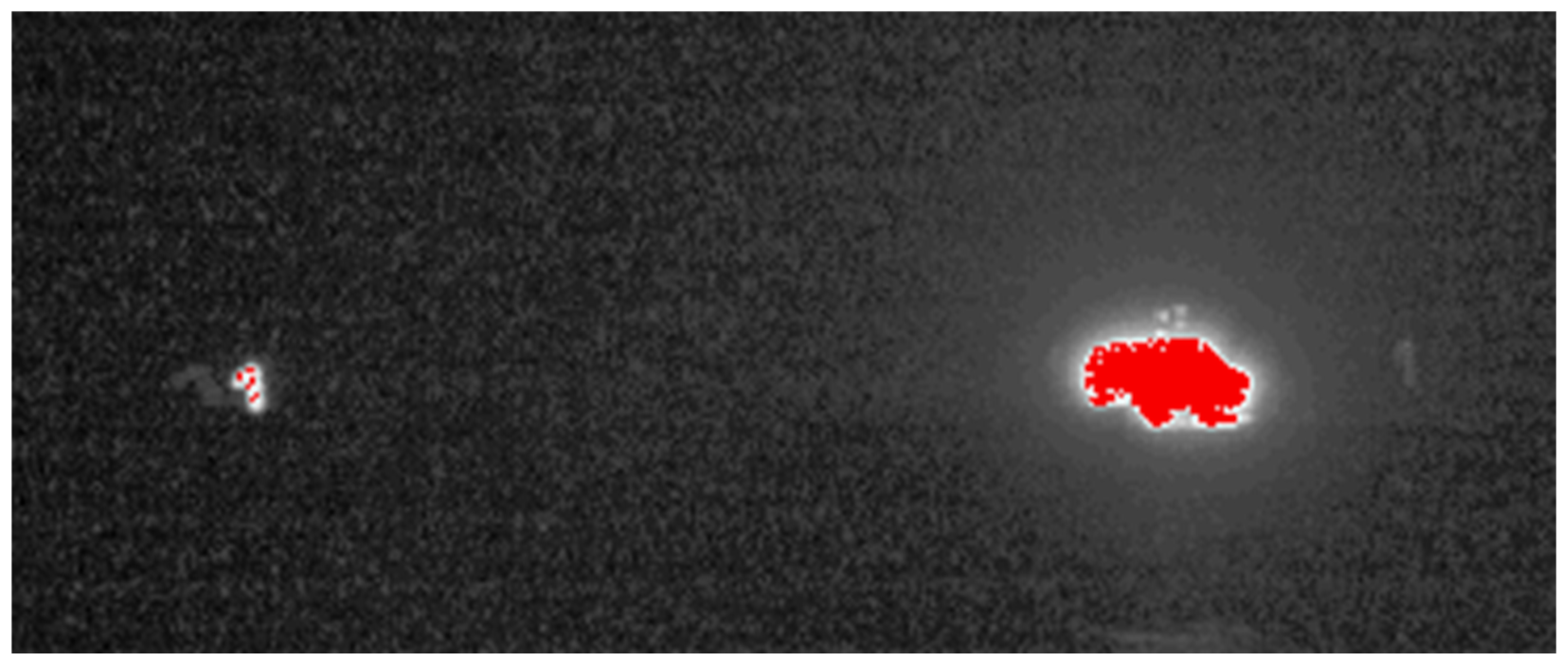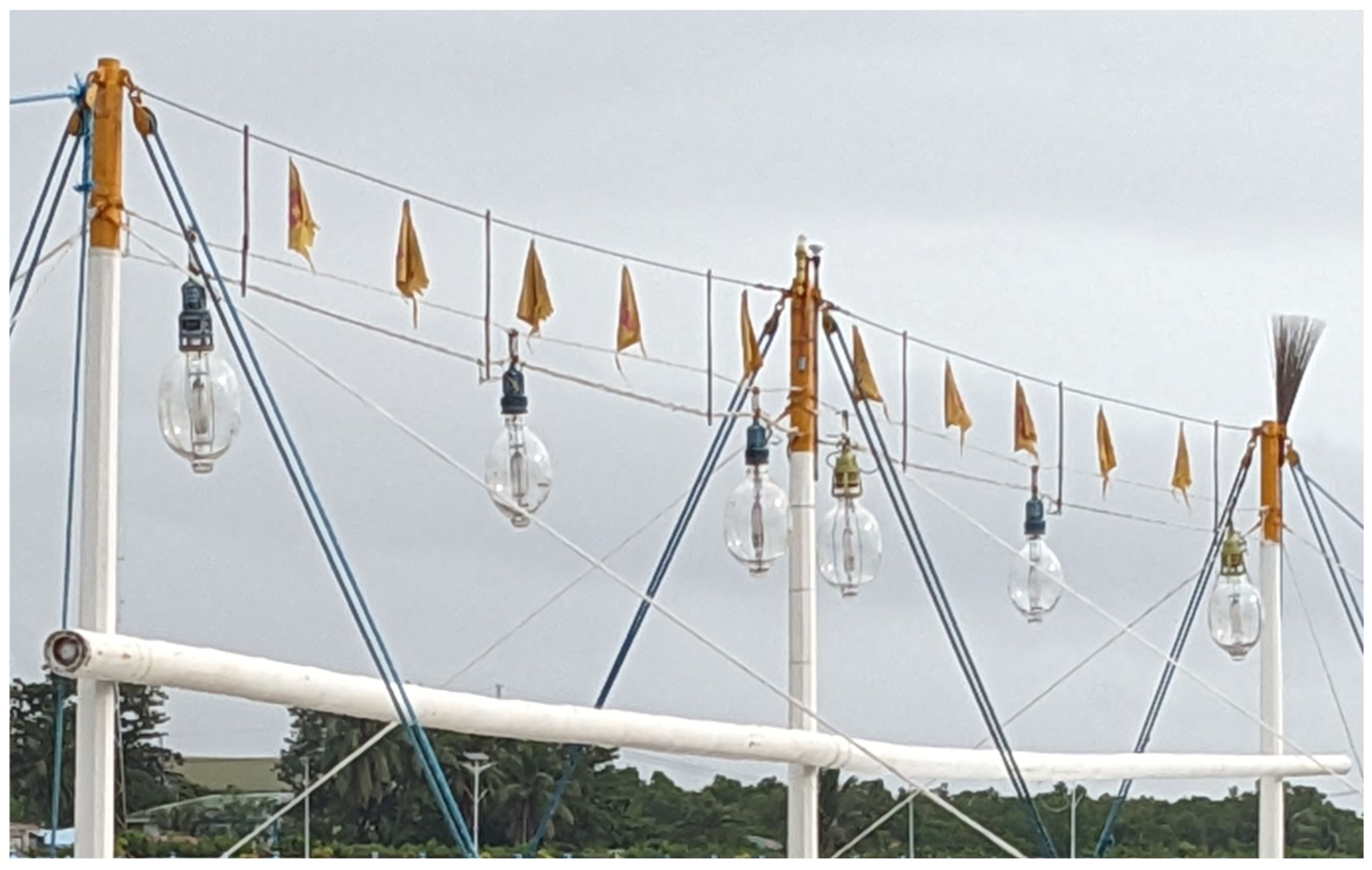Our metal halide collections are described in Appendix A.2 (Figure A27, Figure A28, Figure A29, Figure A30, Figure A31, Figure A32, Figure A33, Figure A34, Figure A35, Figure A36, Figure A37, Figure A38, Figure A39, Figure A40, Figure A41, Figure A42, Figure A43, Figure A44, Figure A45, Figure A46, Figure A47, Figure A48, Figure A49 and Figure A50). Most of the measured metal halides flickered, but we did encounter non-flickering metal halide streetlights in Boulder City, Nevada. Collections on fishing boats equipped with metal halide and quartz halogen spotlights revealed that lighting flickers can even be found at sea (Figure A43, Figure A44, Figure A45, Figure A46, Figure A47, Figure A48, Figure A49 and Figure A50).

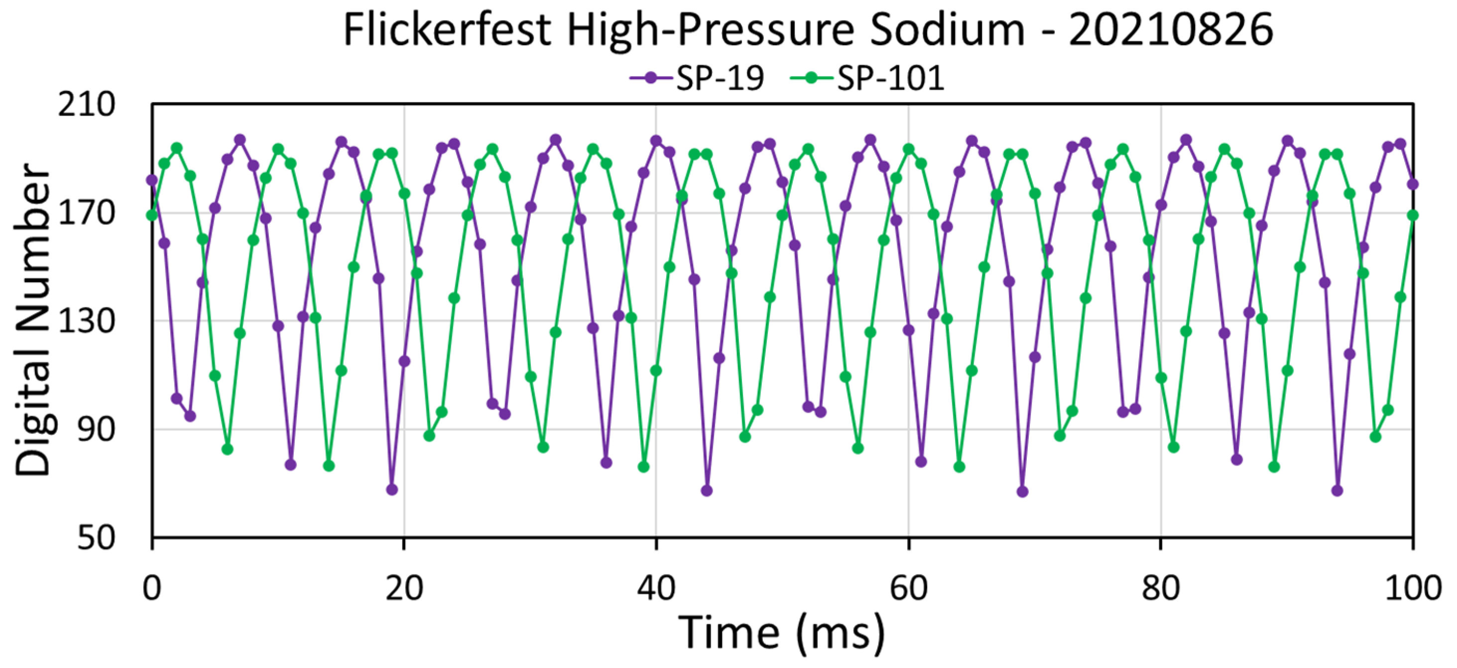
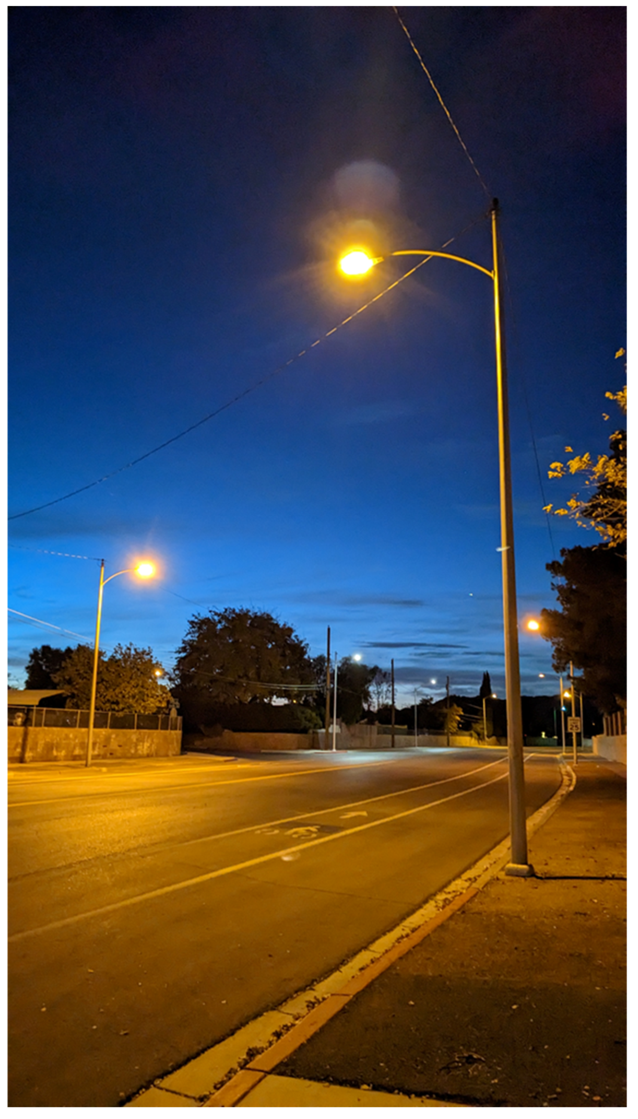
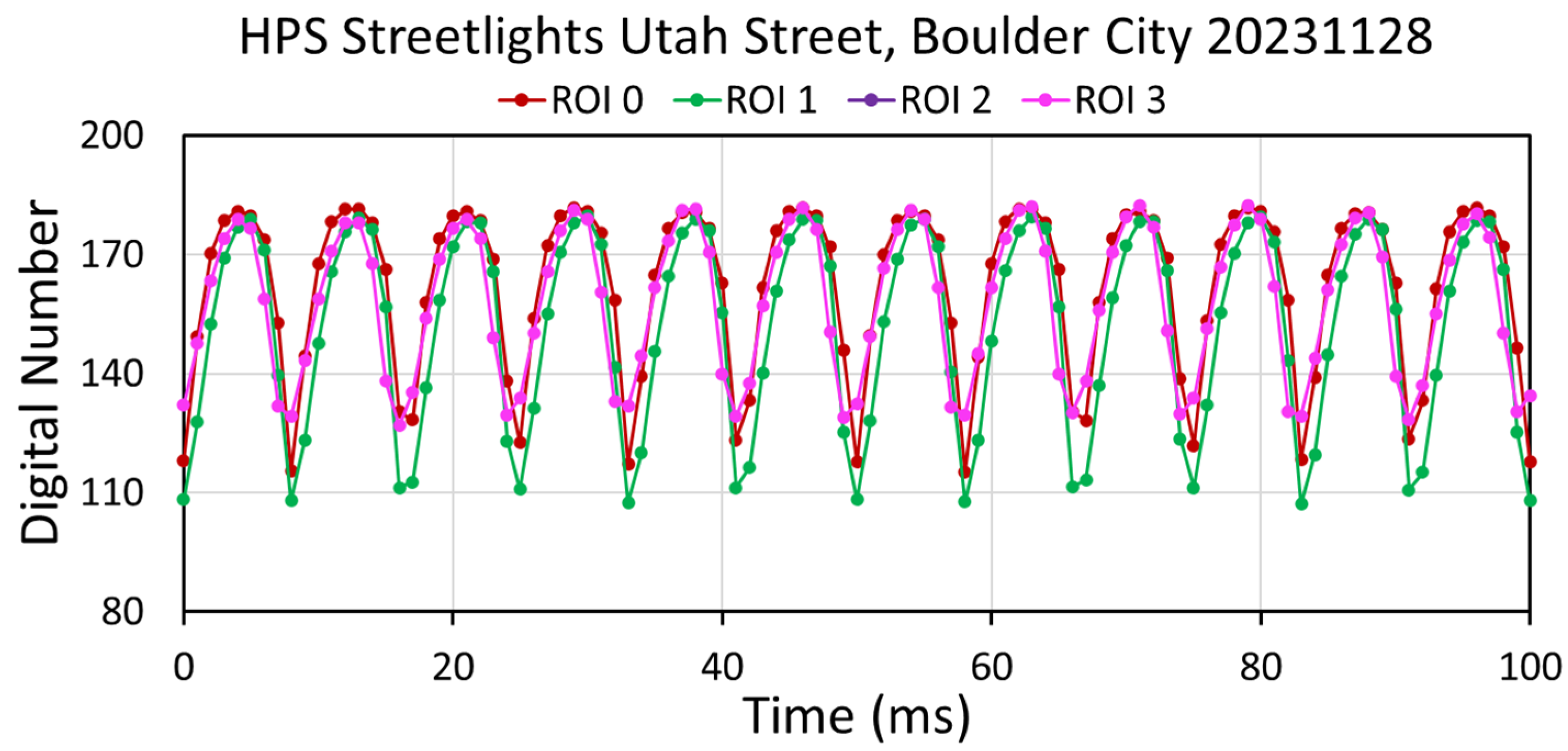
4.3. High-Pressure Sodium (HPS) Luminaires

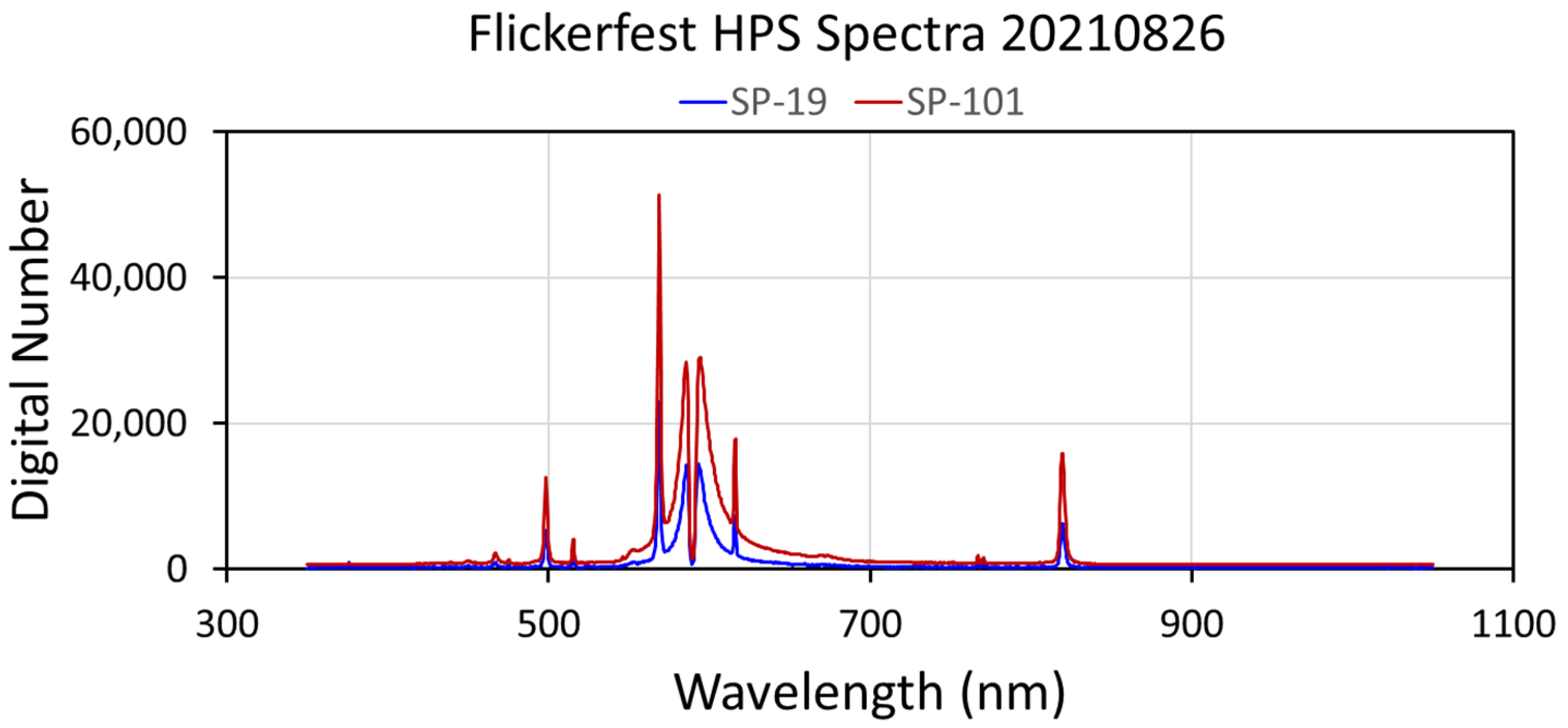
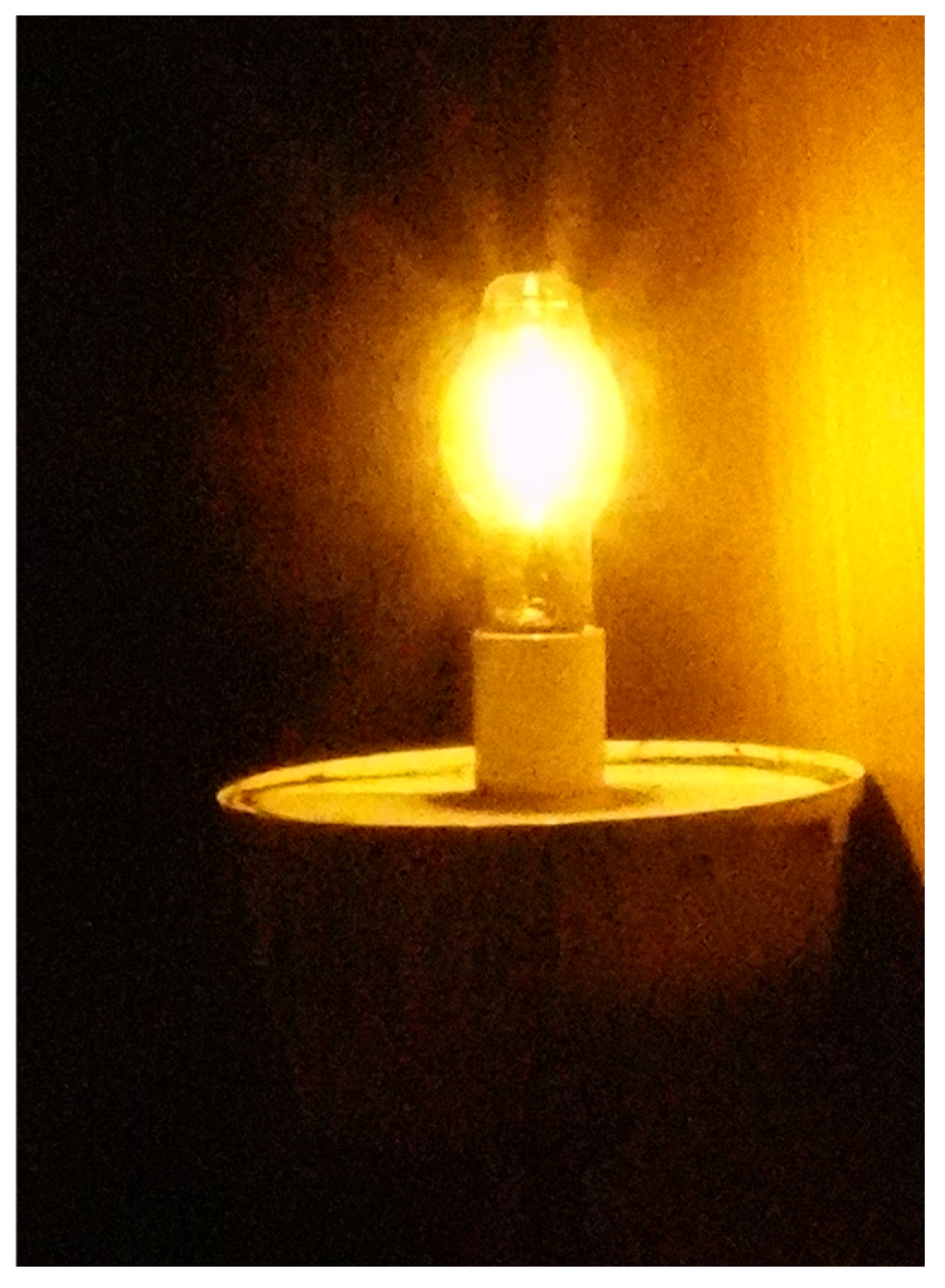
High-pressure sodium luminaires are part of the high-intensity discharge (HID) class of sources that produce light with high-temperature plasma dominated by sodium emission lines [47]. HPS luminaires have a distinctive amber-orange glow that is easily recognizable. Their spectra are dominated by sodium emission lines, with few line emissions on the blue end of the spectrum (Figure A52 and Figure A55). They are faulted for their poor color rendition but appreciated for the lack of blue light emissions by dark sky enthusiasts. HPS lights are gradually being replaced with LED lights. HPS luminaires were measured during Flickerfest in 2021, in Boulder City, Nevada in 2023, and along Highway 1 near the Asian Institute of Technology in 2024. All of the HPS luminaires that we measured showed flicker behavior. This data collection and the corresponding results are described in Appendix A.3 (Figure A51, Figure A52, Figure A53, Figure A54, Figure A55, Figure A56 and Figure A57).

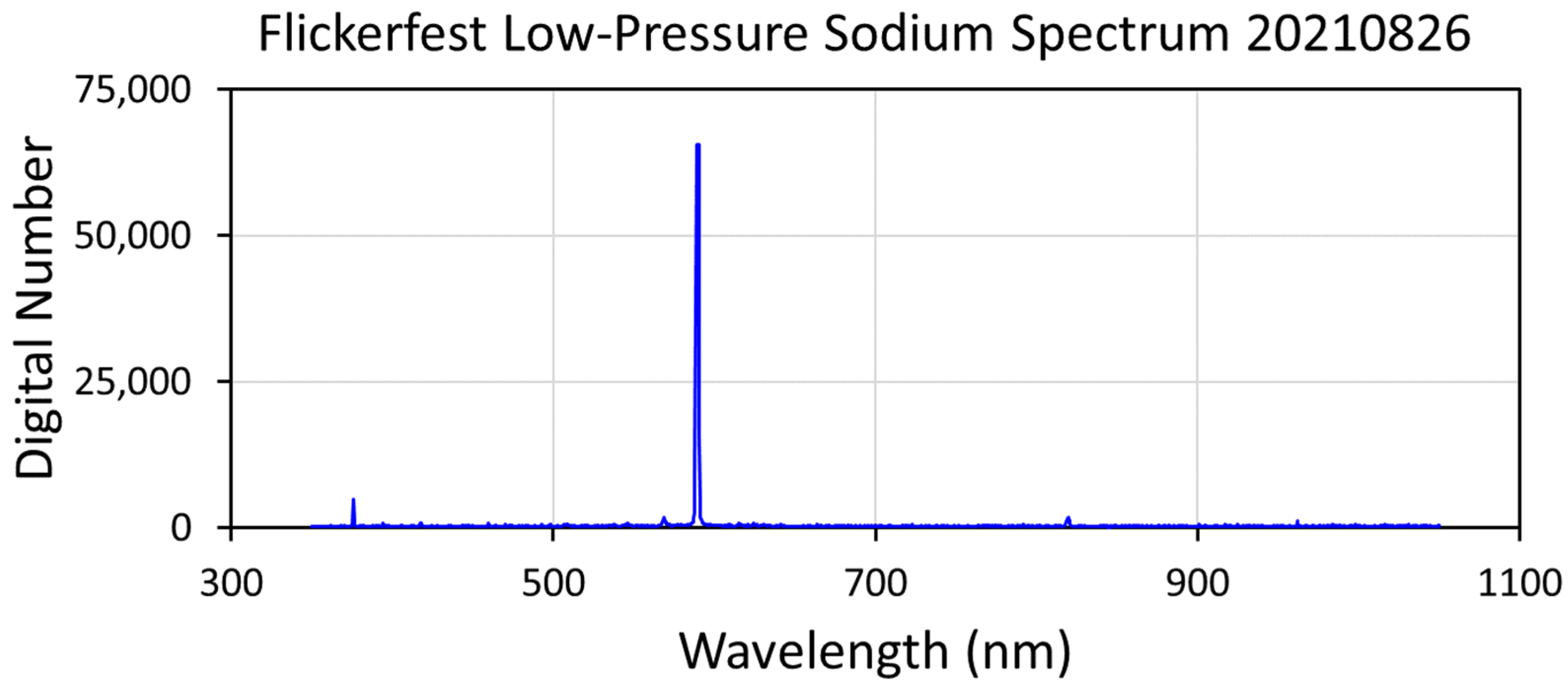
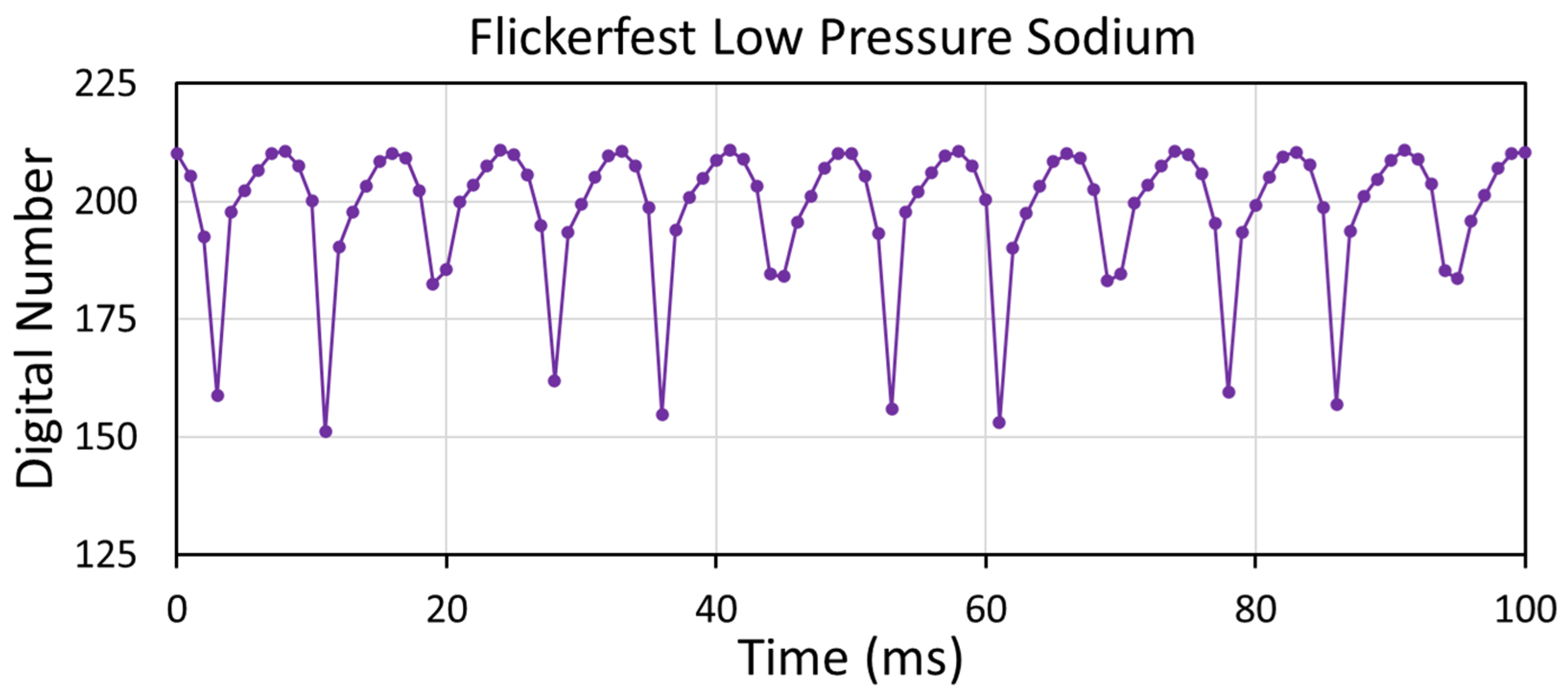
4.4. Low-Pressure Sodium Luminaires

Low-pressure sodium luminaires are uncommon but are commonly found near astronomical observatories in various places around the world. They appear more orange than HPS luminaires (Figure A58). LPS lights are nearly monochromatic, having a prominent sodium line at 590 nm and a minor emission line at 376 nm (Figure A59). The only sample we measured was at Flickerfest and it has a prominent flicker (Figure A60). The production of LPS has ceased in the USA. They continue to be made and sold by a handful of companies outside the USA. The LPS lamp measured at Flickerfest was donated to EOG’s lighting collection by David Keith.

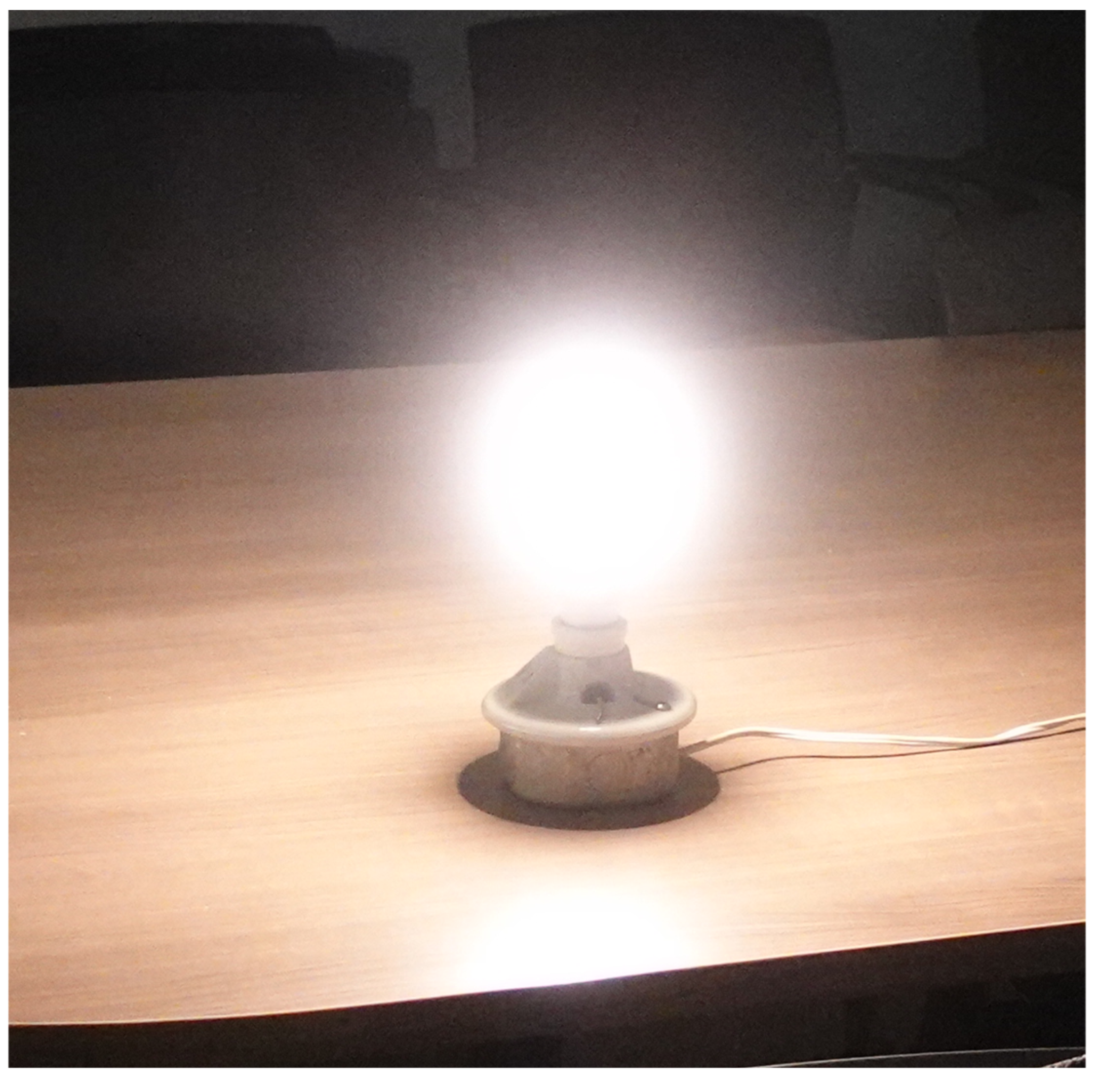
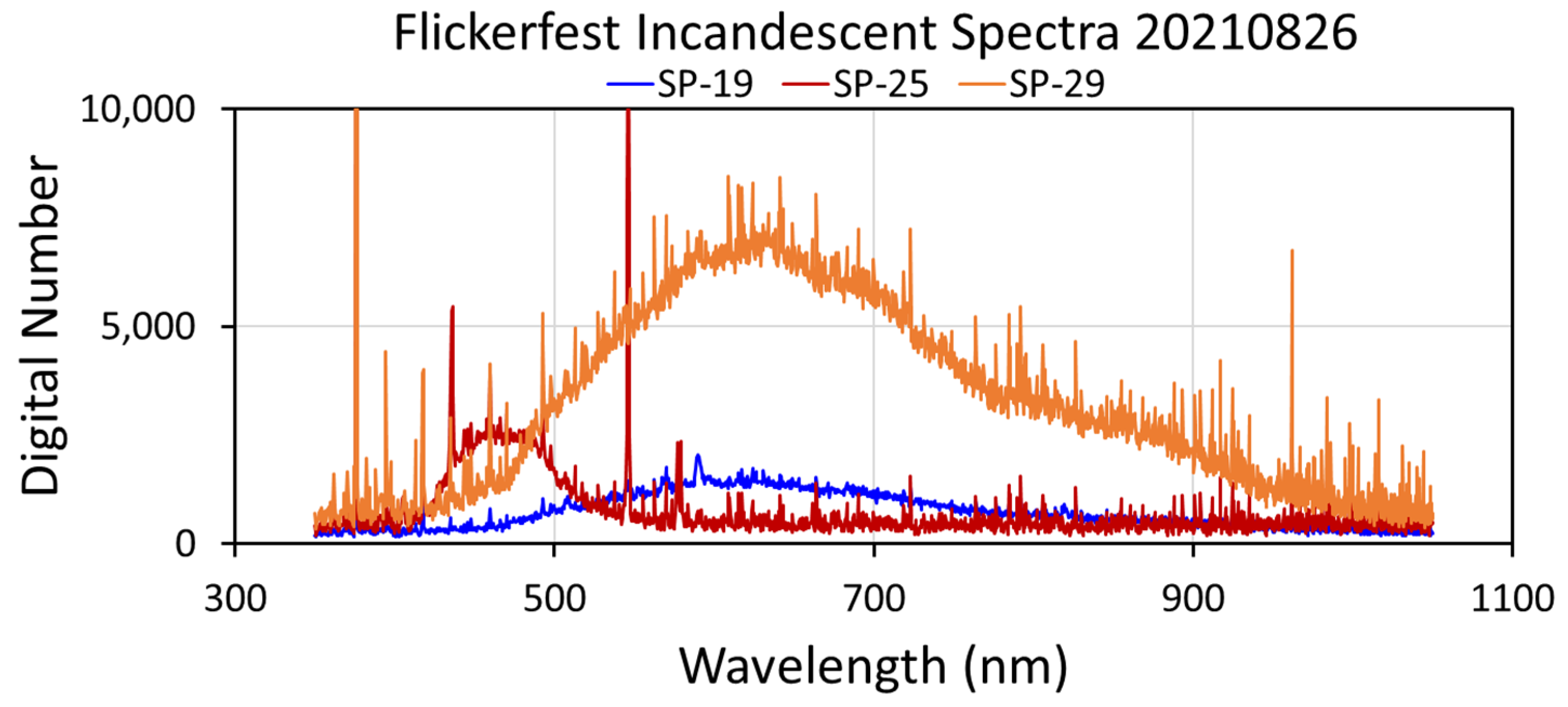
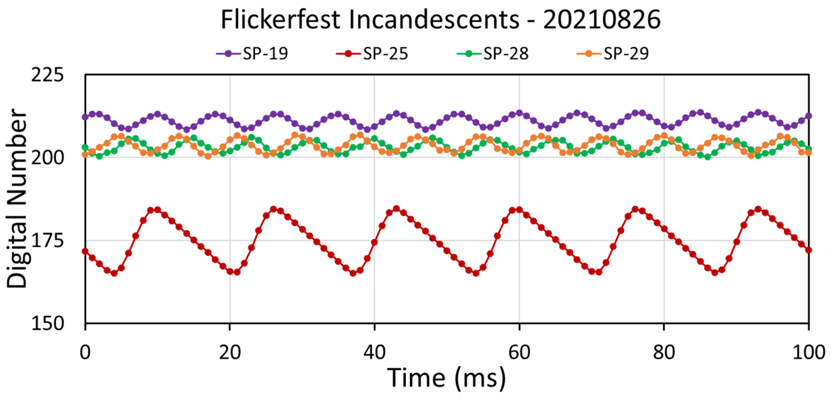
4.5. Incandescent Luminaires

Incandescent luminaires produce light by heating a tungsten filament, resulting in the radiant emissions of photons [48]. Three incandescent lights were measured during Flickerfest 2021. Figure A61 shows a reference photograph of one of these lights. Like LEDs, an incandescent light’s primary output is a broad lobe of light (Figure A62). While LEDs have low radiant outputs beyond 700 nm, incandescent light spectra frequently straddle the visible and near-infrared regions. In contrast, the broad lobe of radiant emissions in incandescent lights typically straddles the visible and near-infrared regions. In some cases, such as quartz halogen, there can be a number of narrow emission lines in incandescent light spectra. All of the incandescent lights that we measured showed flickering behavior (Figure A63). Appendix A.5 contains the details on data collection regarding incandescent lights

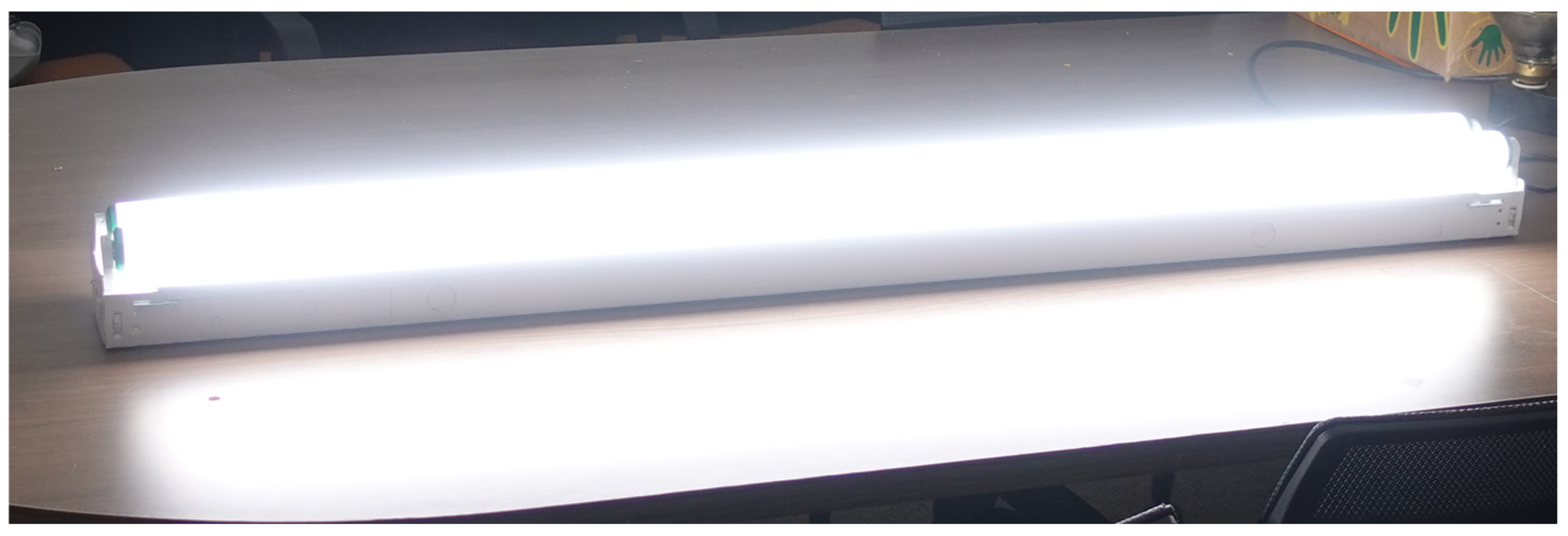
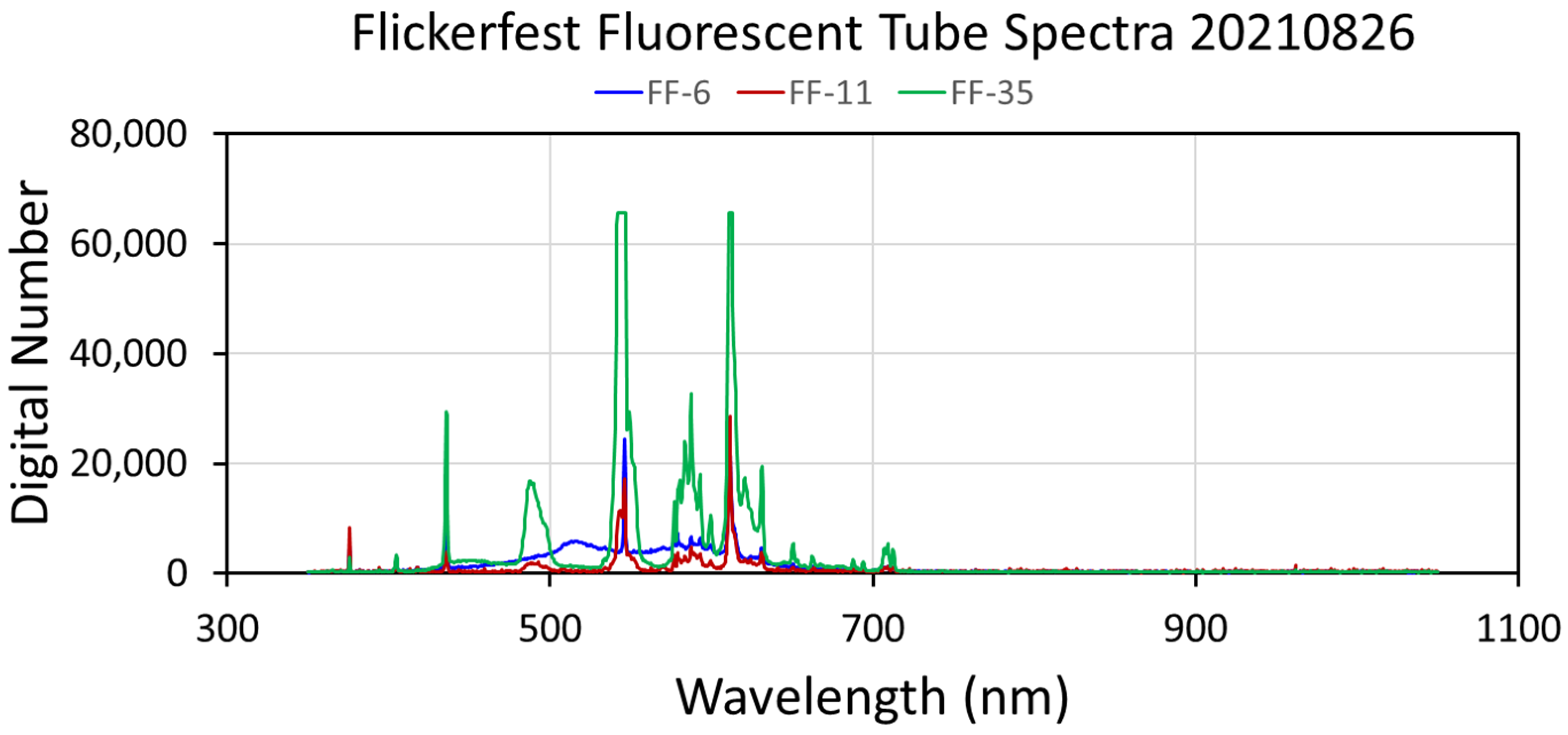
4.6. Fluorescent Luminaires from Flickerfest

Fluorescent lamps use an electrical arc between two cathodes to ionize mercury vapor in a glass tube, forming low-temperature plasma [49]. As excited electrons drop back to lower shells, photons are emitted at UV frequencies. The UV photons are absorbed by the phosphor coating on the interior of the tube, releasing visible light. Figure A64 shows a reference photograph of a pair of four-foot-long fluorescent tubes that we measured. One of the other lights is a desk lamp with two 18 inch tubes, rescued from the trash generated when the NOAA National Geophysical Data Center moved to a new building in 1998. We predict that this lamp may have been manufactured in the 1960s. The third light measured is in the ceiling of EOG’s office suite at the Colorado School of Mines. 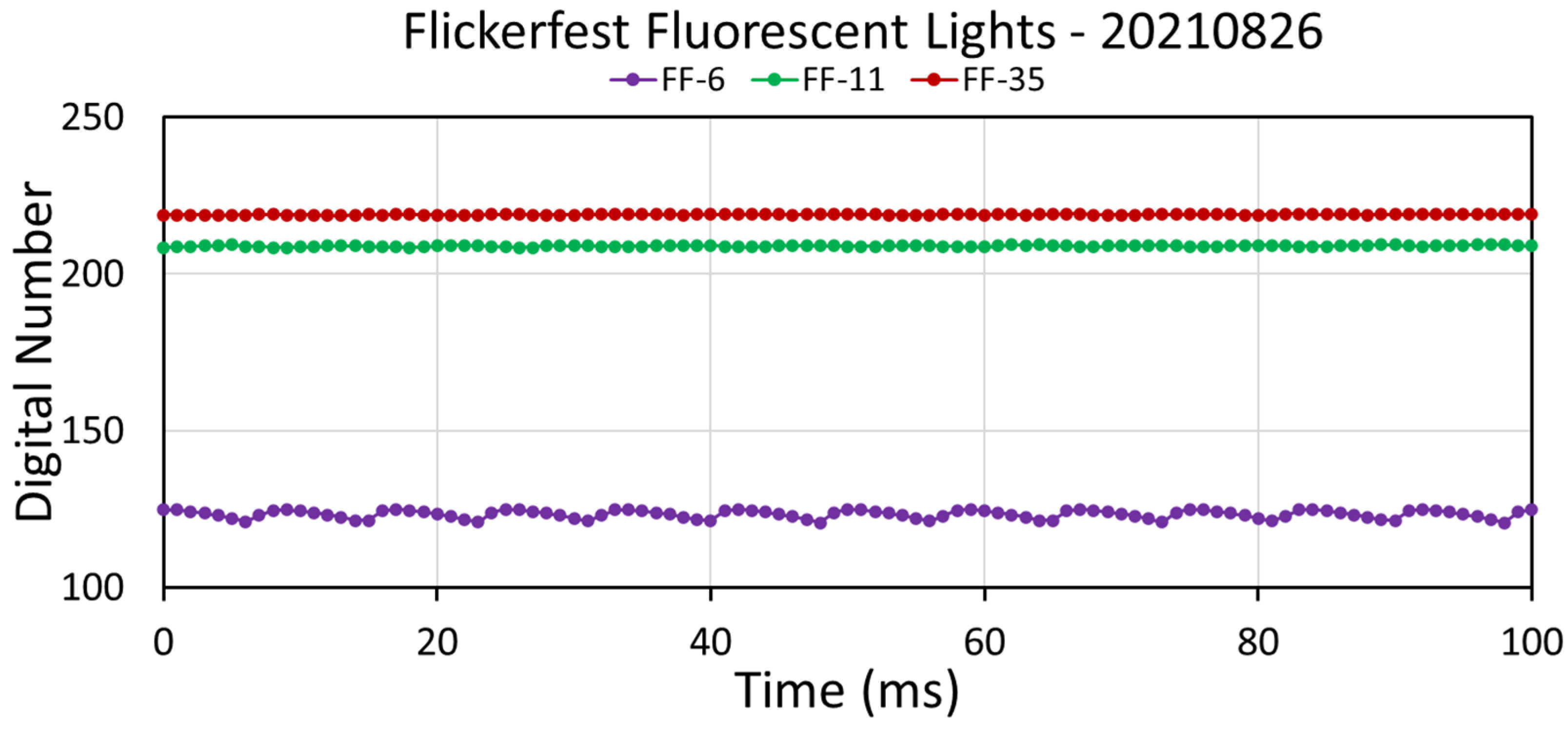Figure A65 shows the spectra of the three lights, which have negligible radiant emissions beyond 700 nm and a series of narrow-band emissions in the visible range. The temporal profiles (Figure A66) show that only one of the lights is obviously flickering. That light is the old desk lamp.

4.7. Compact Fluorescent Luminaires from Flickerfest

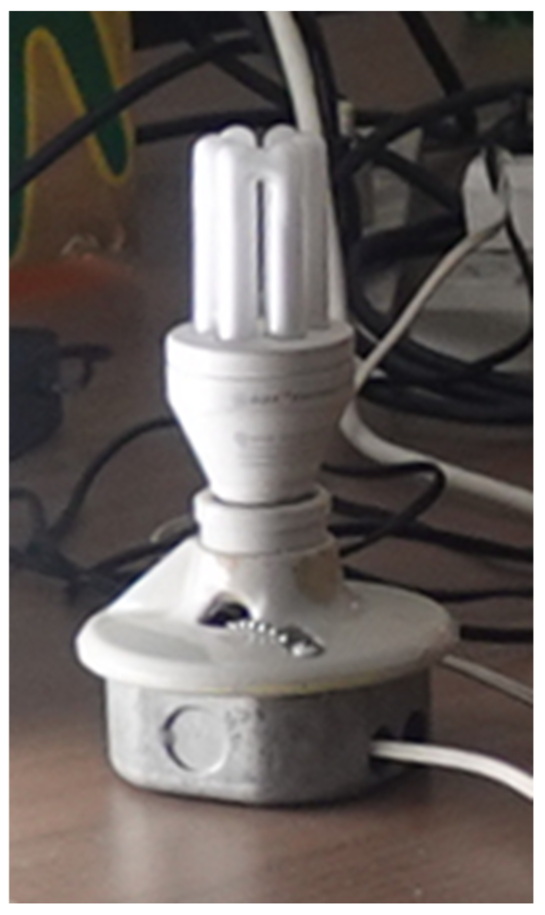
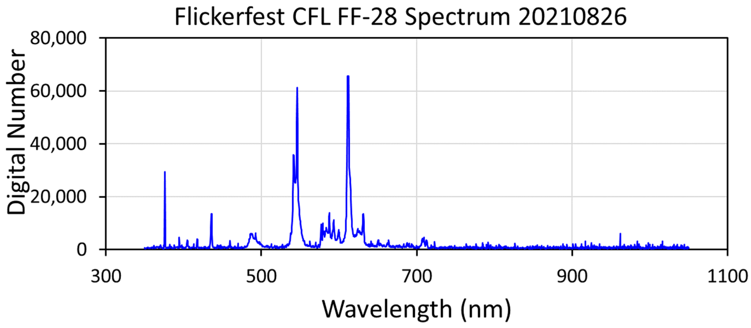
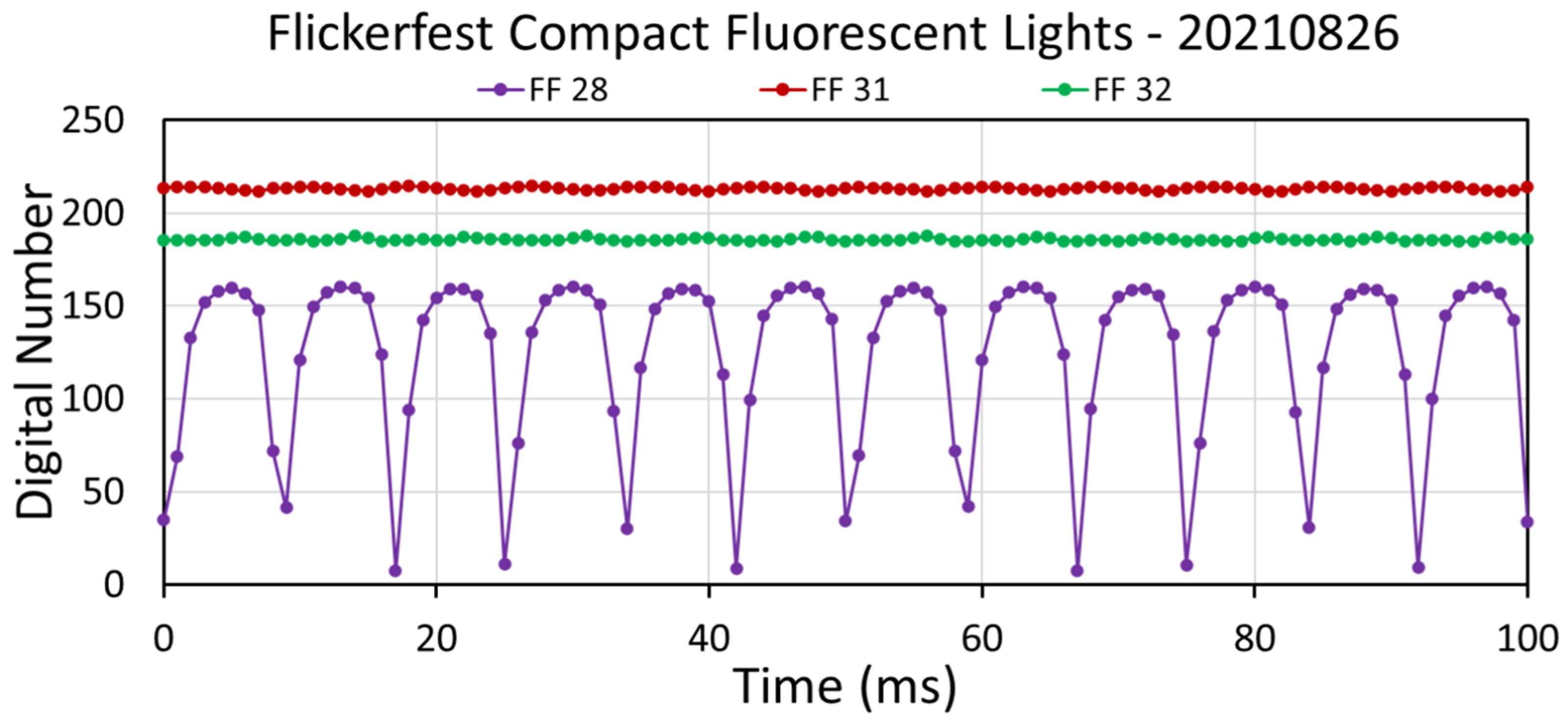
Compact fluorescent luminaires (CFL) are widely used both indoors and outdoors around the world. They operate in the same way as fluorescent tubes, but, in this case, the tubes are curved, and the total volume of tubing is small compared to most fluorescent tubes. Figure A66, Figure A67 and Figure A68 show a reference photo, spectrum, and temporal profiles of CFL bulbs measured at Flickerfest 2021. One of the downsides of both fluorescent and compact fluorescent luminaires is the presence of mercury, which can escape to the environment when a tube breaks or is improperly disposed of. Over time, they are being supplanted by LED lights.

4.8. Flicker Synchronization

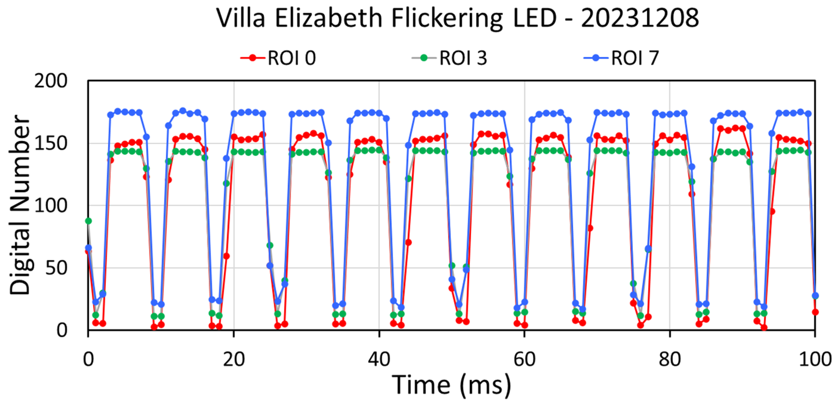
Flicker synchronization is common at the site level with LED, metal halide, and high- pressure sodium lights. The easiest way to identify flicker synchronization is to stack temporal profiles from individual high-speed camera collections. Flicker synchronization was observed in the LED sources from the following locations: Henderson, Nevada (Figure A7, Figure A12, Figure A13 and Figure A19); Villa Elizabeth, Philippines (Figure A25 and Figure A41); and Boulder City, Nevada (Figure A32 and Figure A56). HPS and LED flicker synchronization is also present along Highway 1 outside the AIT campus.

4.9. Reducing Saturation with Neutral Density Filters

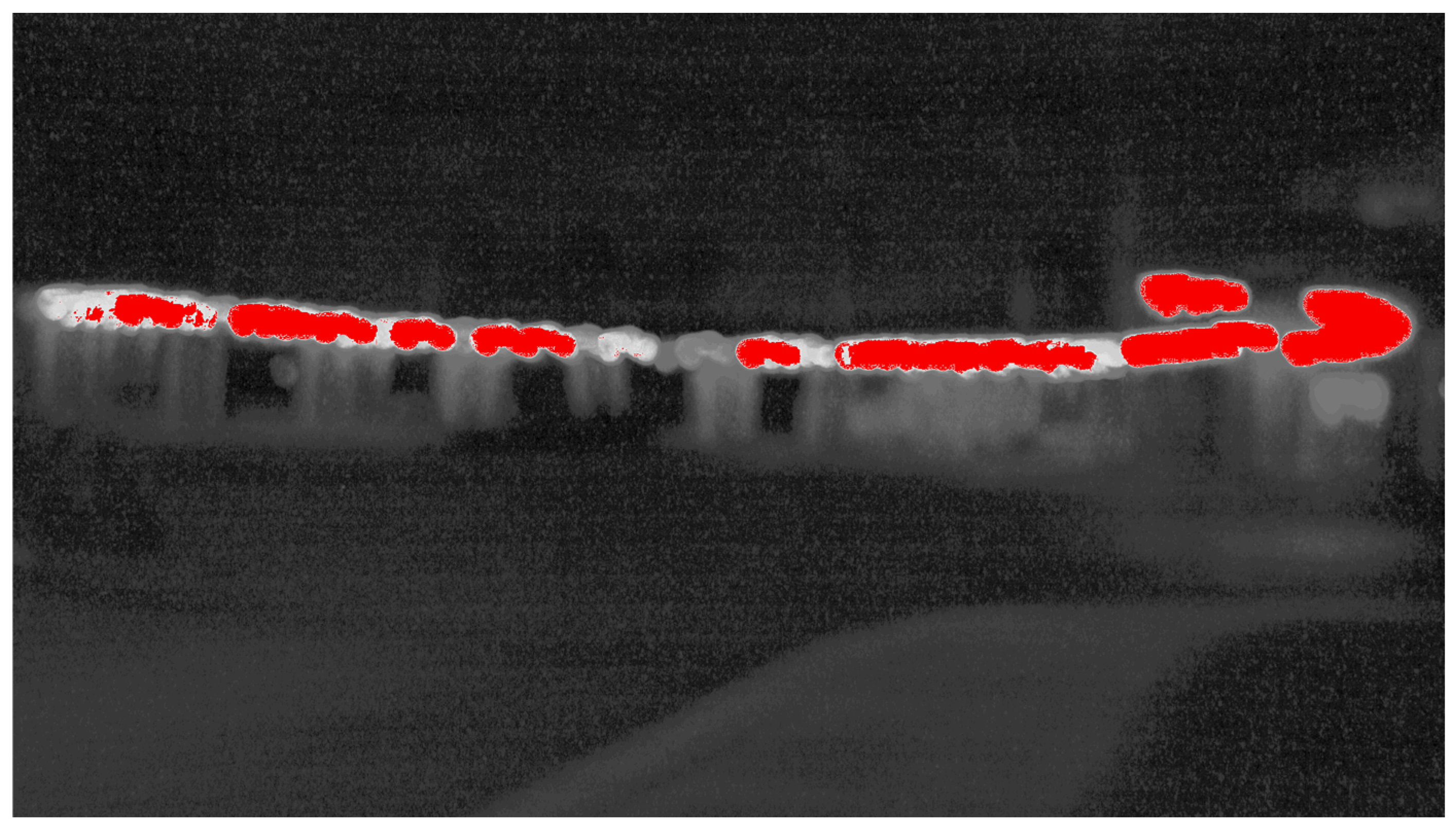
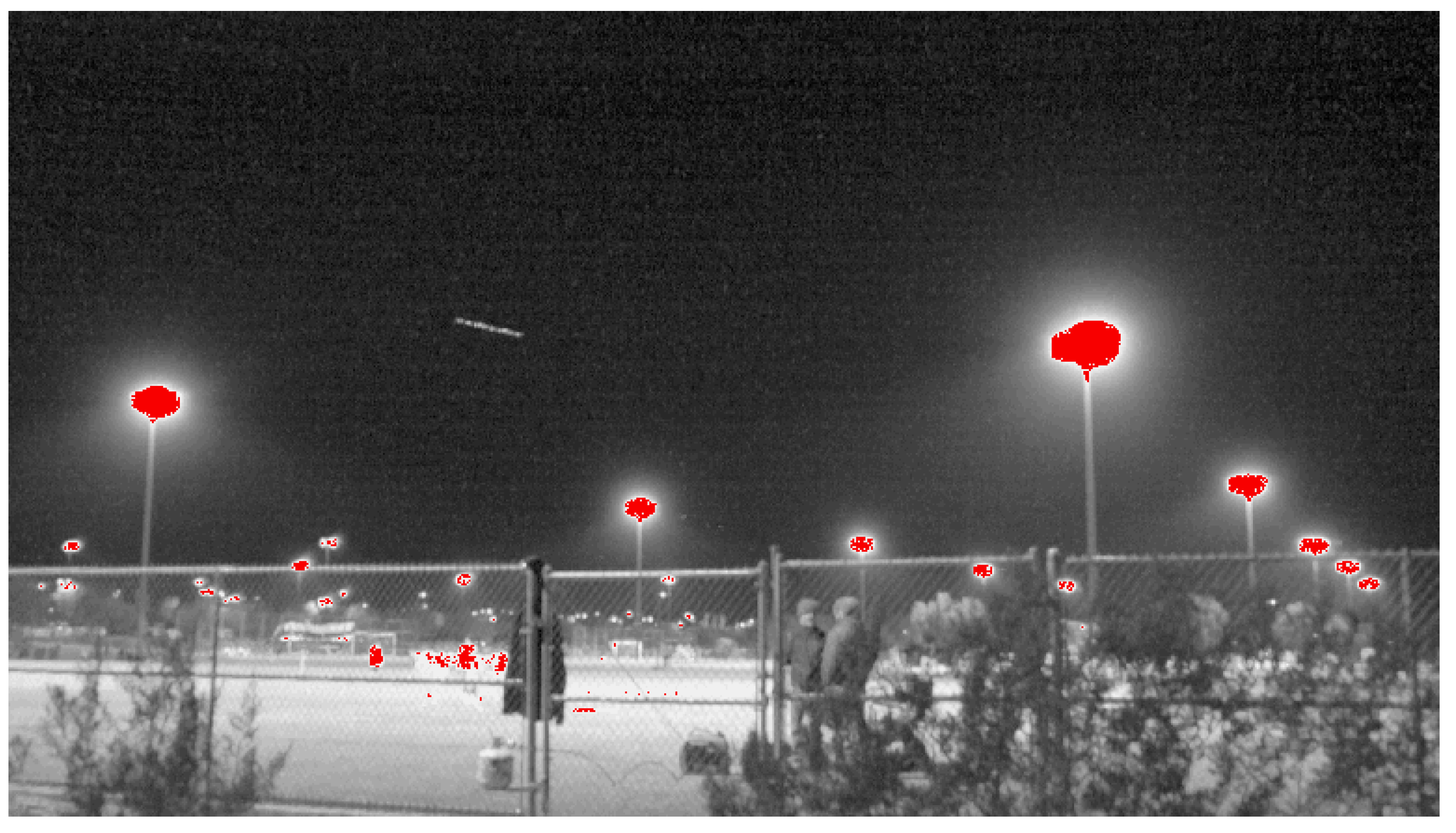
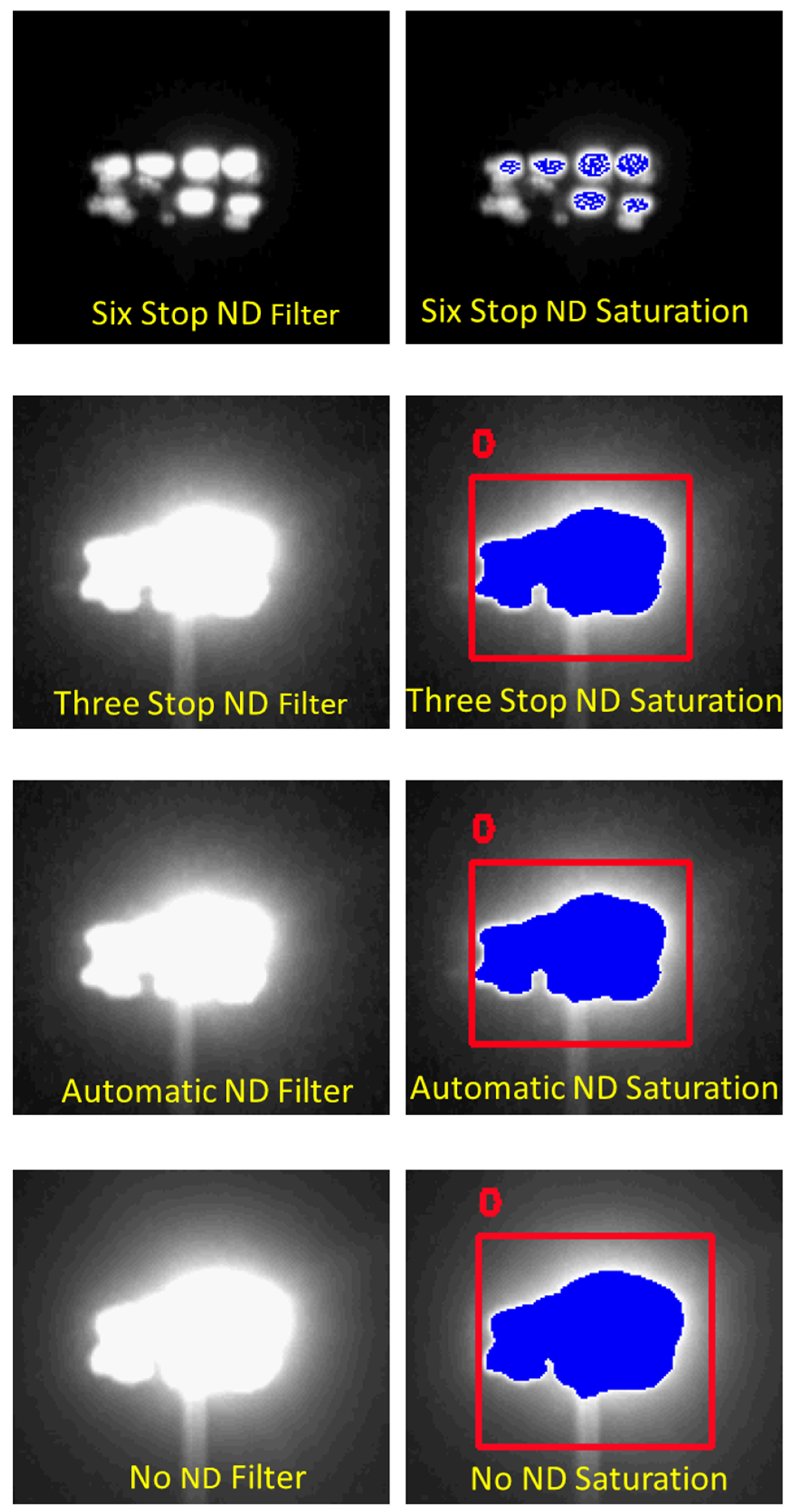
The maximum count images from each MP4 collection were tested for the presence of saturation by color coding DN = 255 as a specific color. Saturation at peak radiant output was found in many of the lights measured without a neutral density (Figure A9, Figure A16, Figure A20, Figure A24, Figure A34, Figure A38, Figure A44, Figure A46 and Figure A57). To examine the reduction in saturation via neutral density filters, collections were taken from a Heritage Park metal halide cluster with five neutral density filter settings: (1) no neutral density filter; (2) Sony camera automatic neutral density filter; (3) Sony camera three-stop neutral density filter (12.5% transmissivity); (4) external six-stop neutral density filter (1.56% transmissivity); and (5) external 16.5-stop neutral density filter (0.001% transmissivity). No lighting was detected when the 16.5-stop ND filter was used.

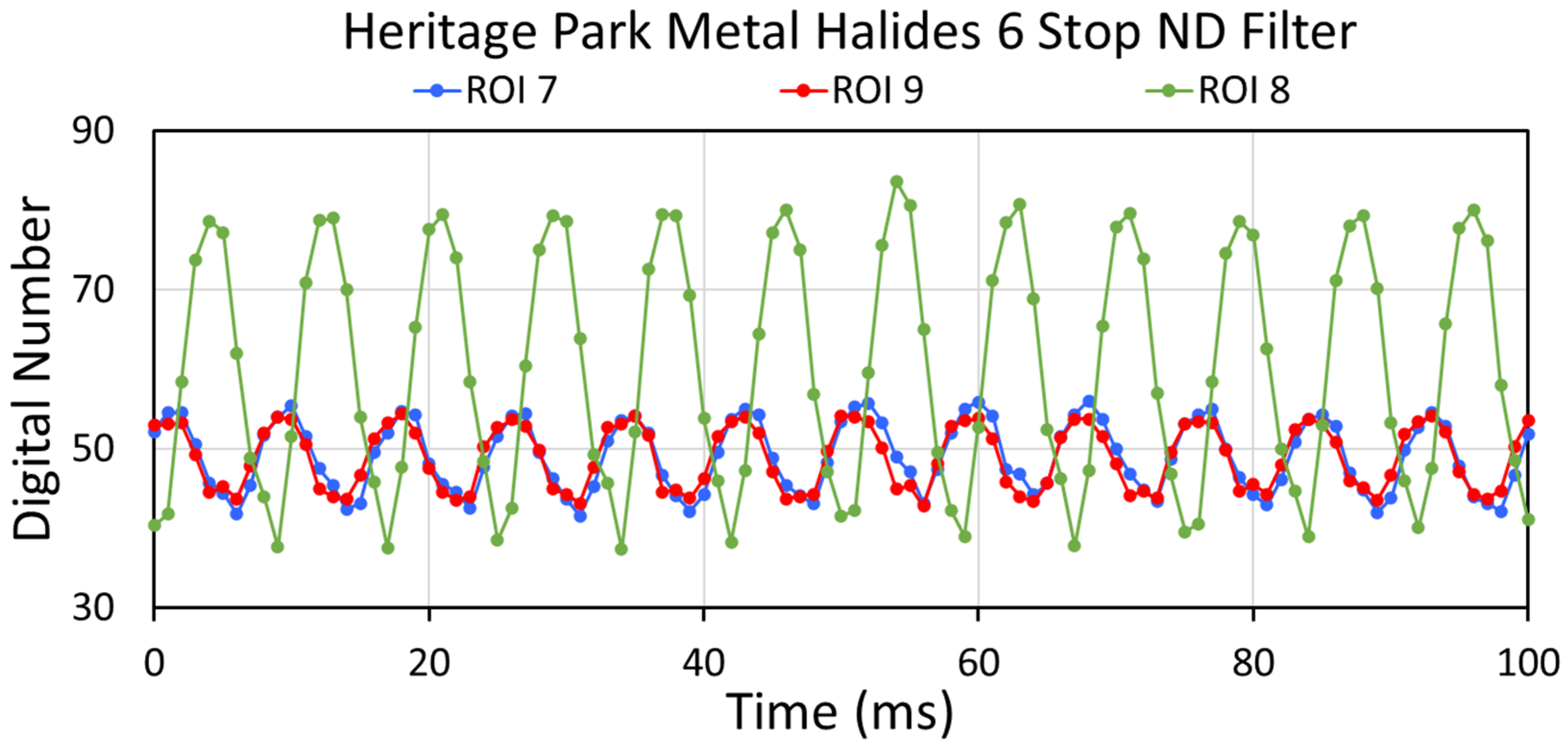
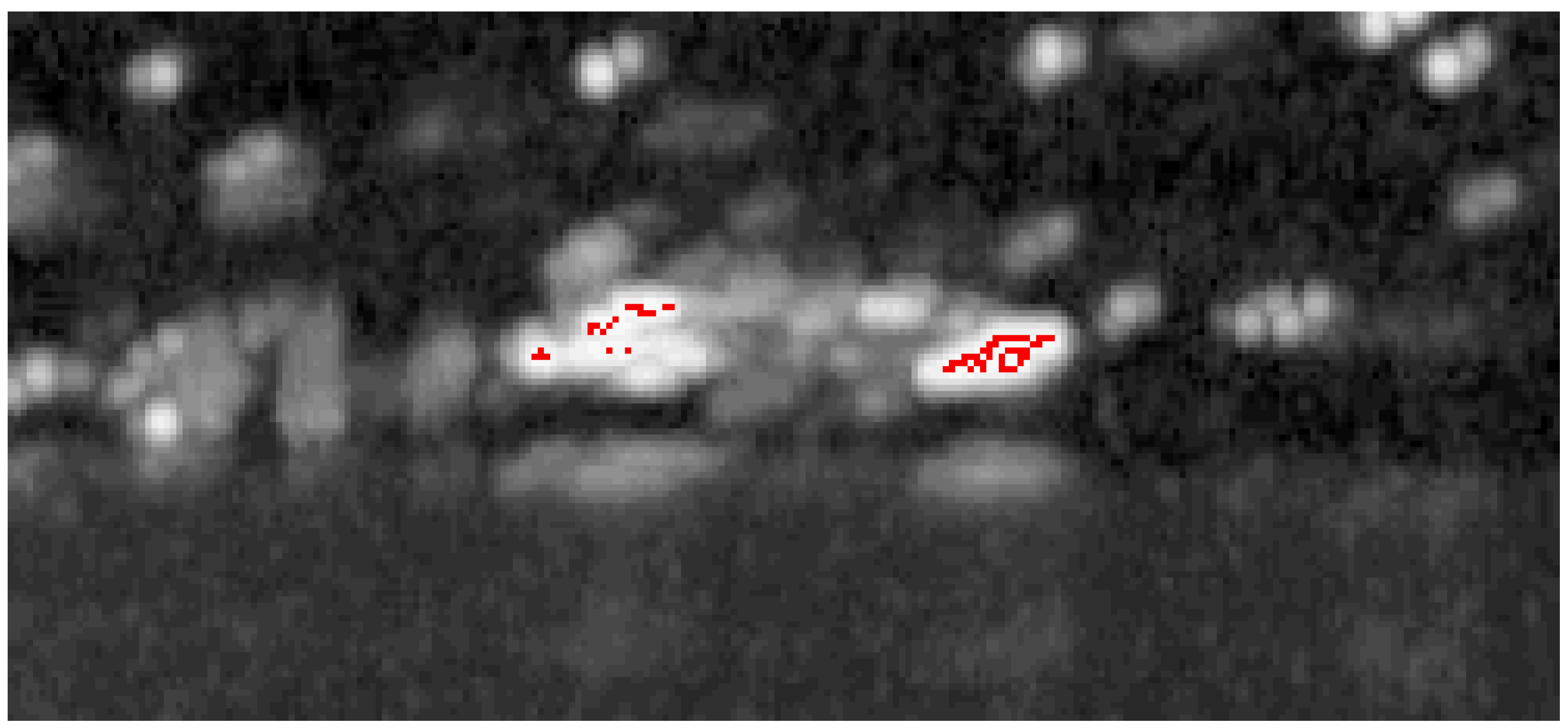
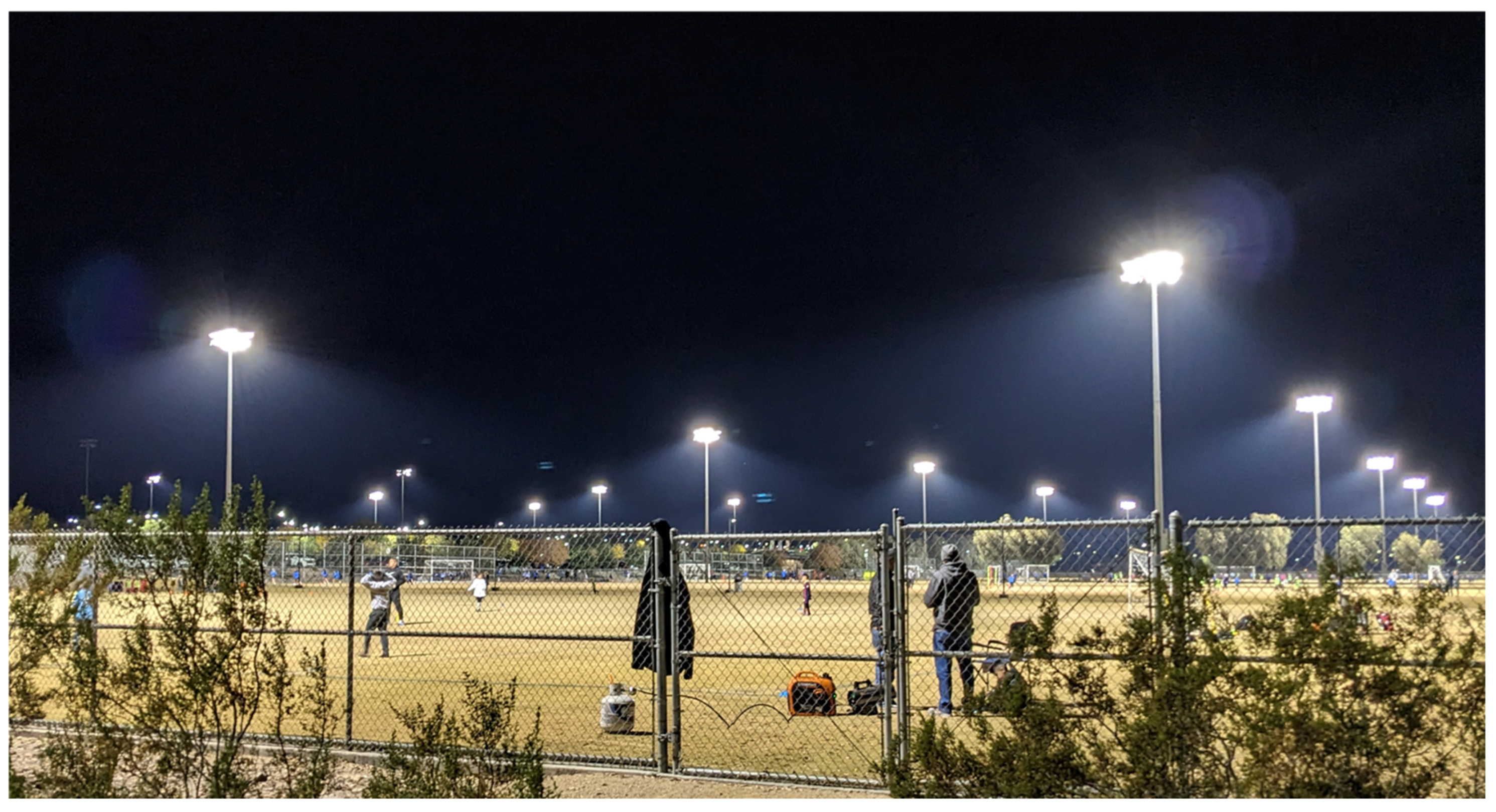
Figure 5 shows the area of saturation present in the MP4 data with four different neutral density filter settings for the cluster of metal halide luminaires on the pole closest to the camera at Heritage Park. Saturated pixels are color coded with blue. There is a large irregularly shaped saturation blob present in the no-ND, automatic-ND, and three-stop ND collections. The same saturation blob was found in earlier MP4 collections of the same site conducted without a neutral density filter (Figure A38). The three red boxes marked “0” were drawn by the MP4 processing system for profile extraction. The entire contents of the red boxes were used to construct the temporal profiles. The irregular shape of the saturation in Figure 5 indicates that there are multiple bright saturated luminaires inside each blob. The area of saturation contracted only slightly going from no-ND to the automatic-ND filter and to the three-stop ND filter.

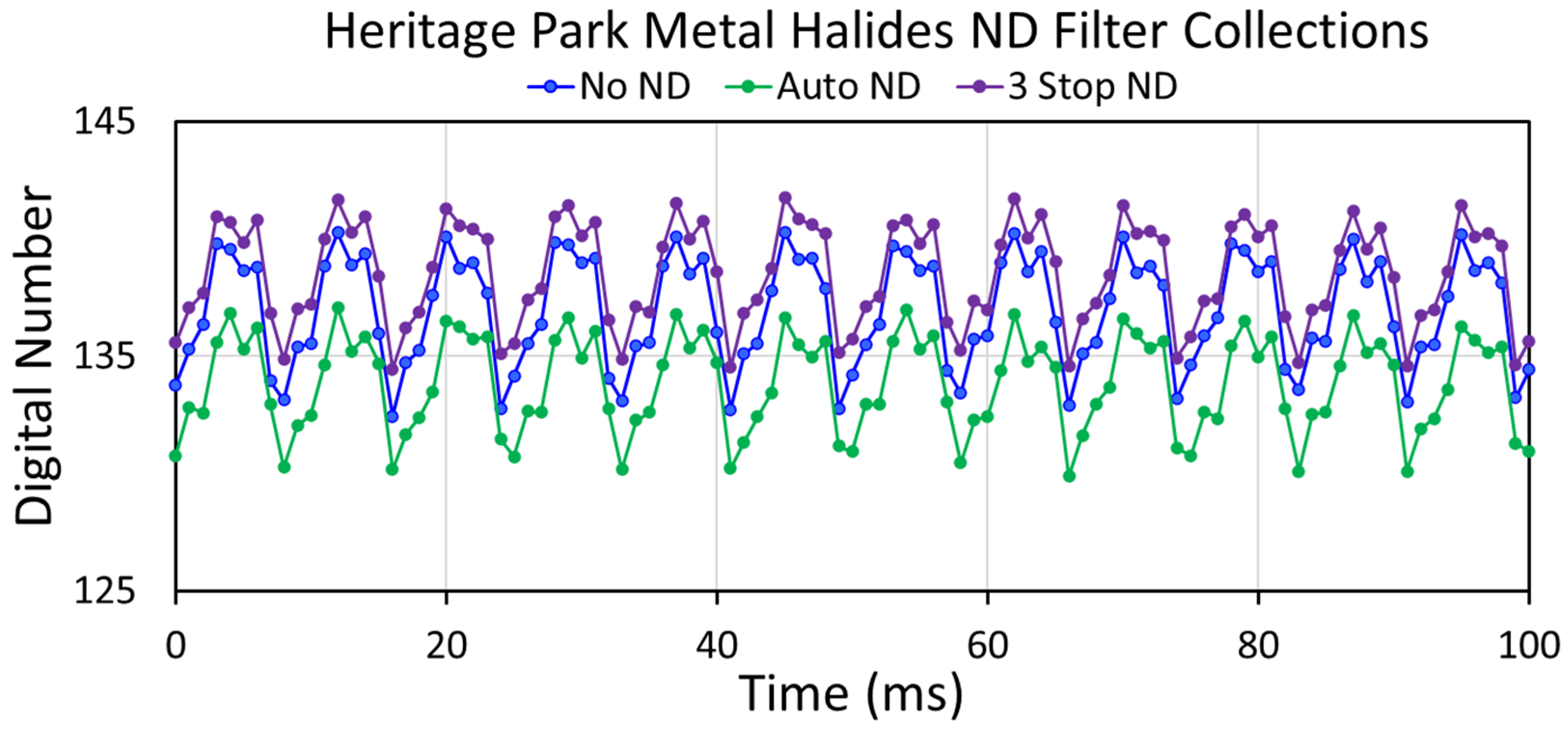
Figure 6 shows the temporal profiles for lighting cluster “0” from the no-ND, automatic-ND, and three-stop ND settings. These appear very similar to the temporal profiles from the original collection performed on these luminaires with a no-ND filter (Figure A36, Figure A37 and Figure A39). The profiles show flicker, but the amplitude is dampened by saturation during the peak part of the flicker cycling. Another factor contributing to a dampening of the flicker cycling is the lack of synchronization among the lights inside the saturation blobs. The profiles have a jagged appearance, which is a tip-off indicating partial destructive interference from multiple unsynchronized luminaires present in the cluster. The peak count is near 135—far below the saturation level of 255. This is due to the inclusion of glow and background pixels inside the rectangular sampling area. The temporal profiles in Figure 6 are not synchronized because they come from three separate MP4 collections.

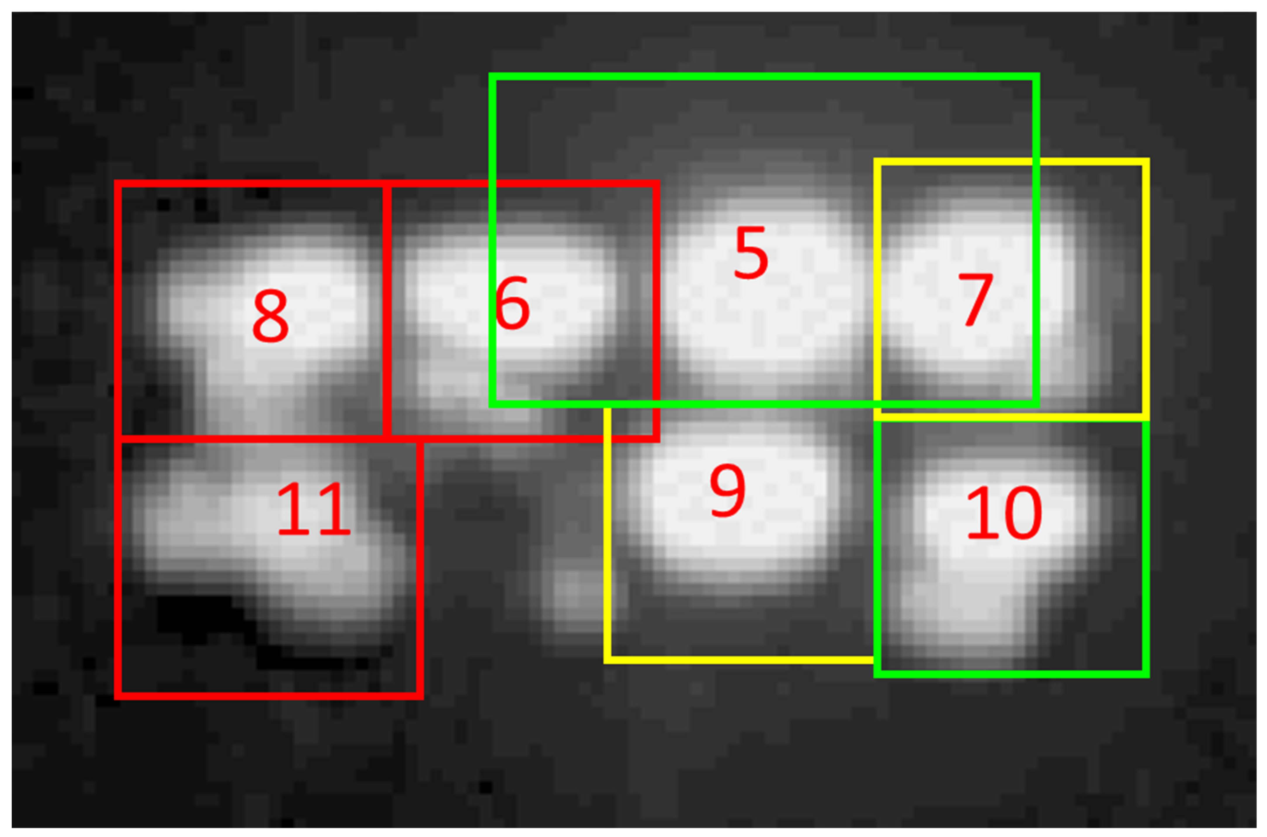
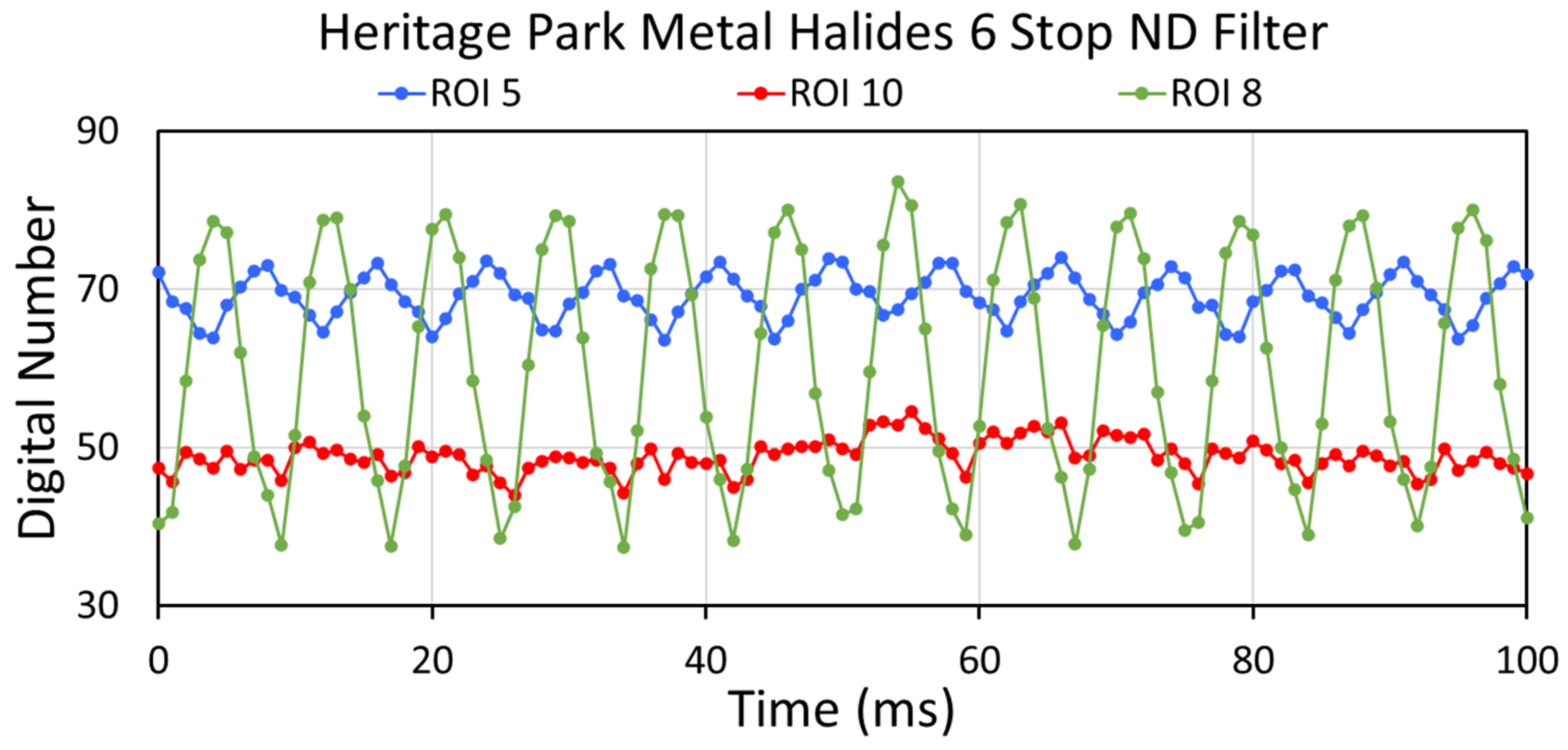
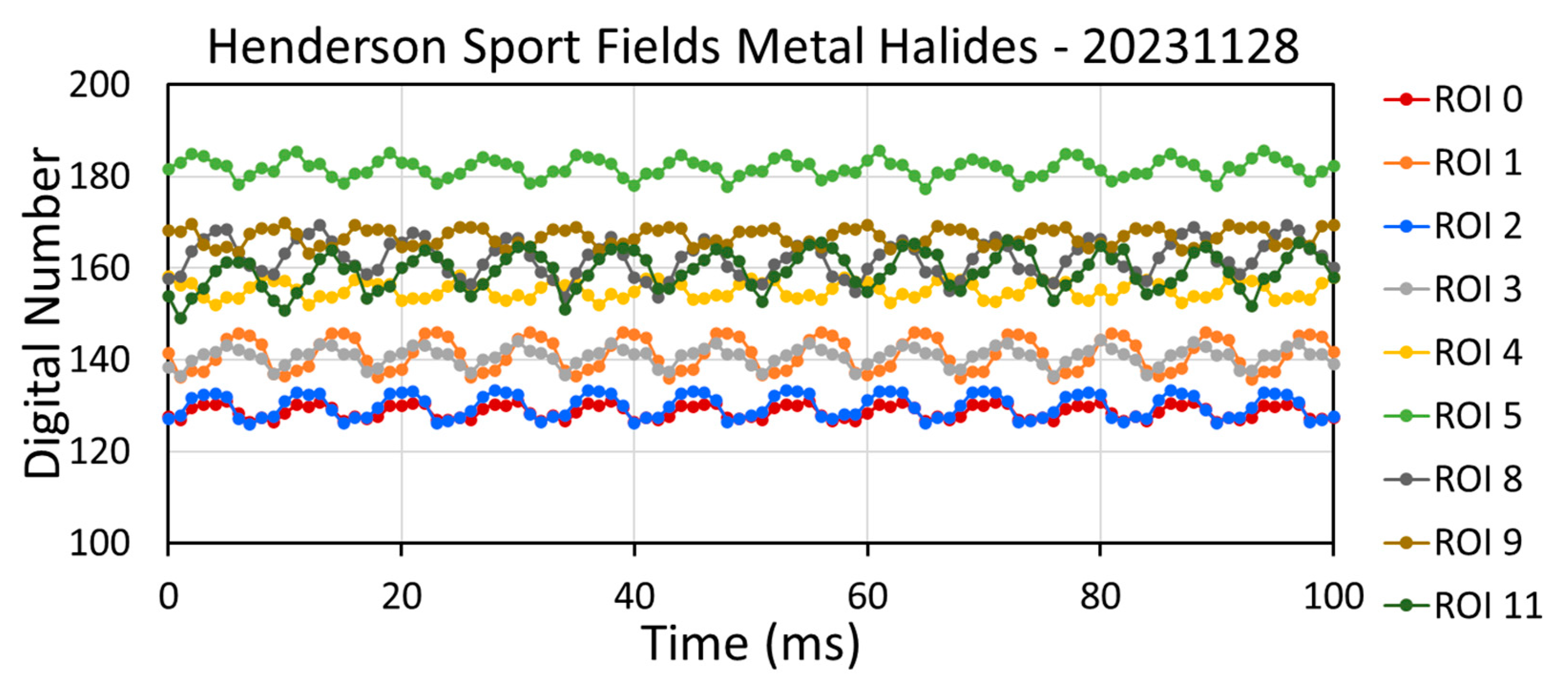
In contrast, seven individual lighting clusters and very little saturation are found in the collection made with the six-stop neutral density filter (Figure 7). Cluster number 9 appears as a single luminaire, with a symmetrical round lighting feature and no side lobes. Five clusters (6, 7, 8, 10, and 11) have lobes on the sides, indicating that two or more luminaires have been combined in a single temporal profile. Cluster 5 straddles three light sources.

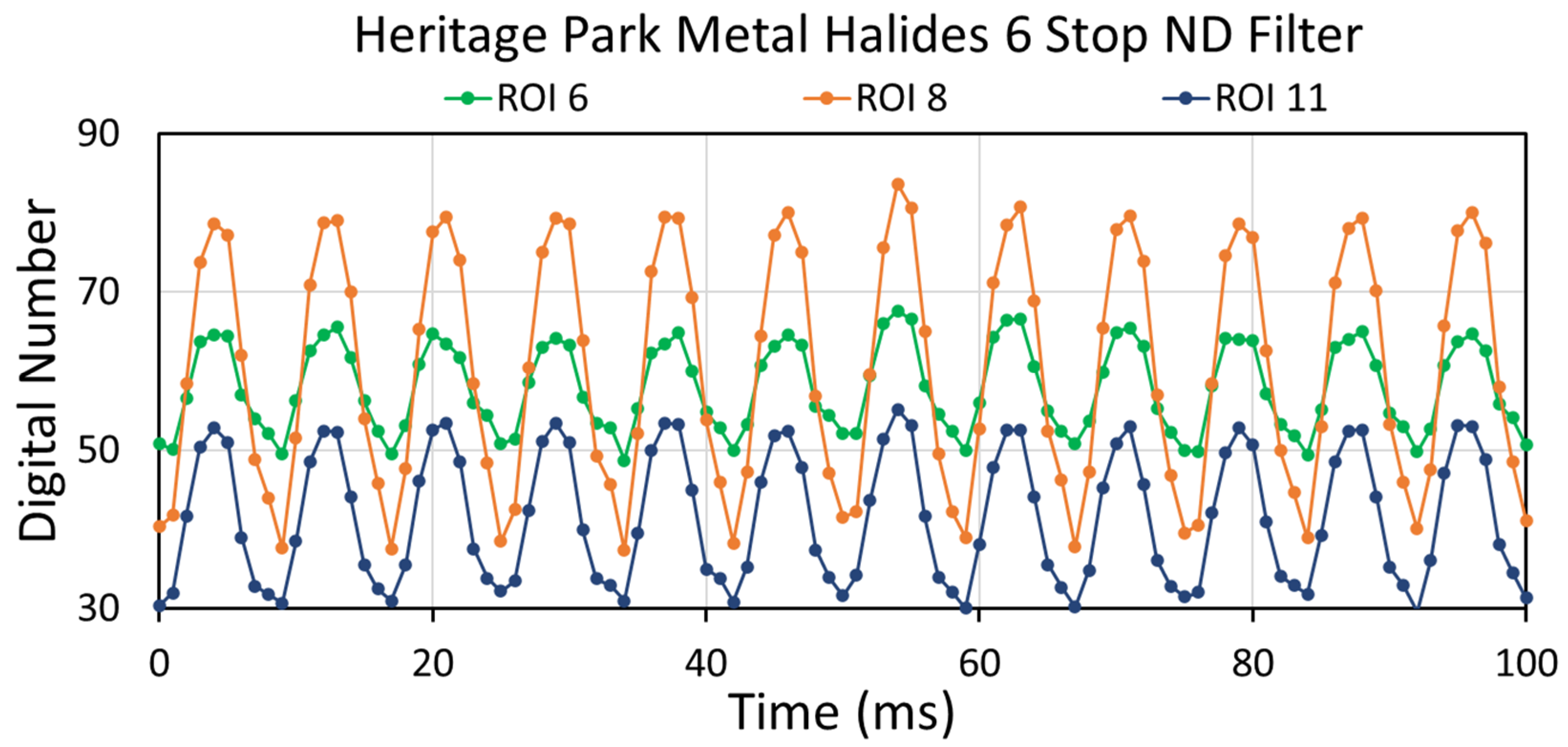
Figure 8 shows temporal profiles for three synchronized lighting clusters (6, 8, and 11) from the six-stop ND collection. The flicker amplitudes are high and lack the multiple jagged features seen in the saturated profiles (Figure 6), attributed to partial destructive interference. Two other lights (7 and 9) show synchronization with each other but lower amplitude (Figure 9). In addition, there are two outlier temporal profiles from clusters 5 and 10 (Figure 10). Cluster 5 shows the classic sawtooth pattern found when mixing light from two non-synchronized sources (Figure A14 and Figure A15). Cluster 10’s temporal profile is similar to those from the saturated clusters from the no-ND, automatic-ND, and three-stop ND collections. This indicates the mixing of light from several unsynchronized sources.

4.10. Detection of Flicker with a Spectrometer

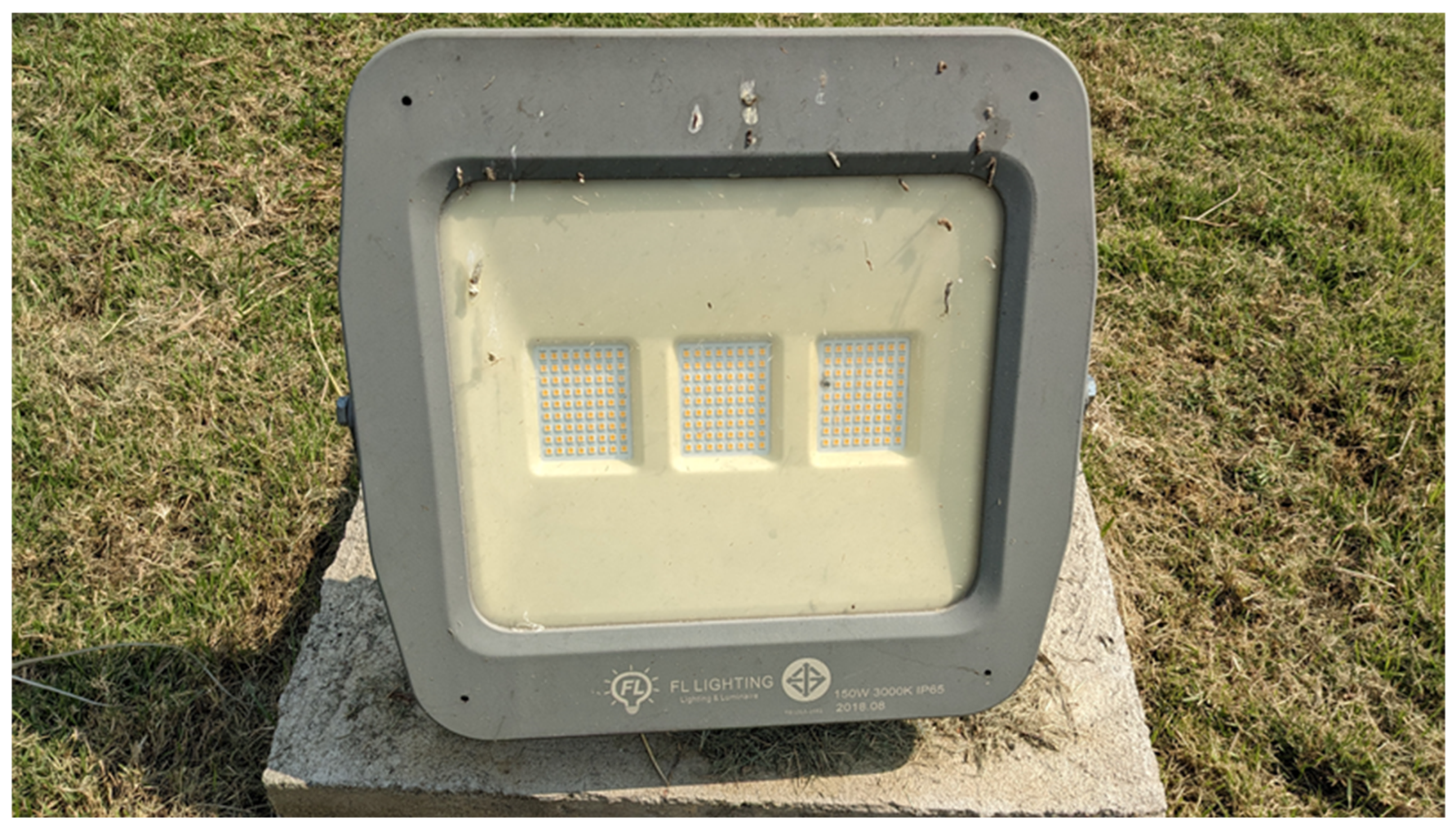
Normally, the integration time on a spectrometer is set to a half to a full second to avoid the collection of unsteady spectra associated with flicker. By including multiple flicker cycles in the integration time, the effects of flicker are intentionally avoided. To explore the possibility that flicker can be detected with a spectrometer, we collected one hundred spectra of two flicking light sources with the USB4000’s shortest possible integration time of 3.8 ms. 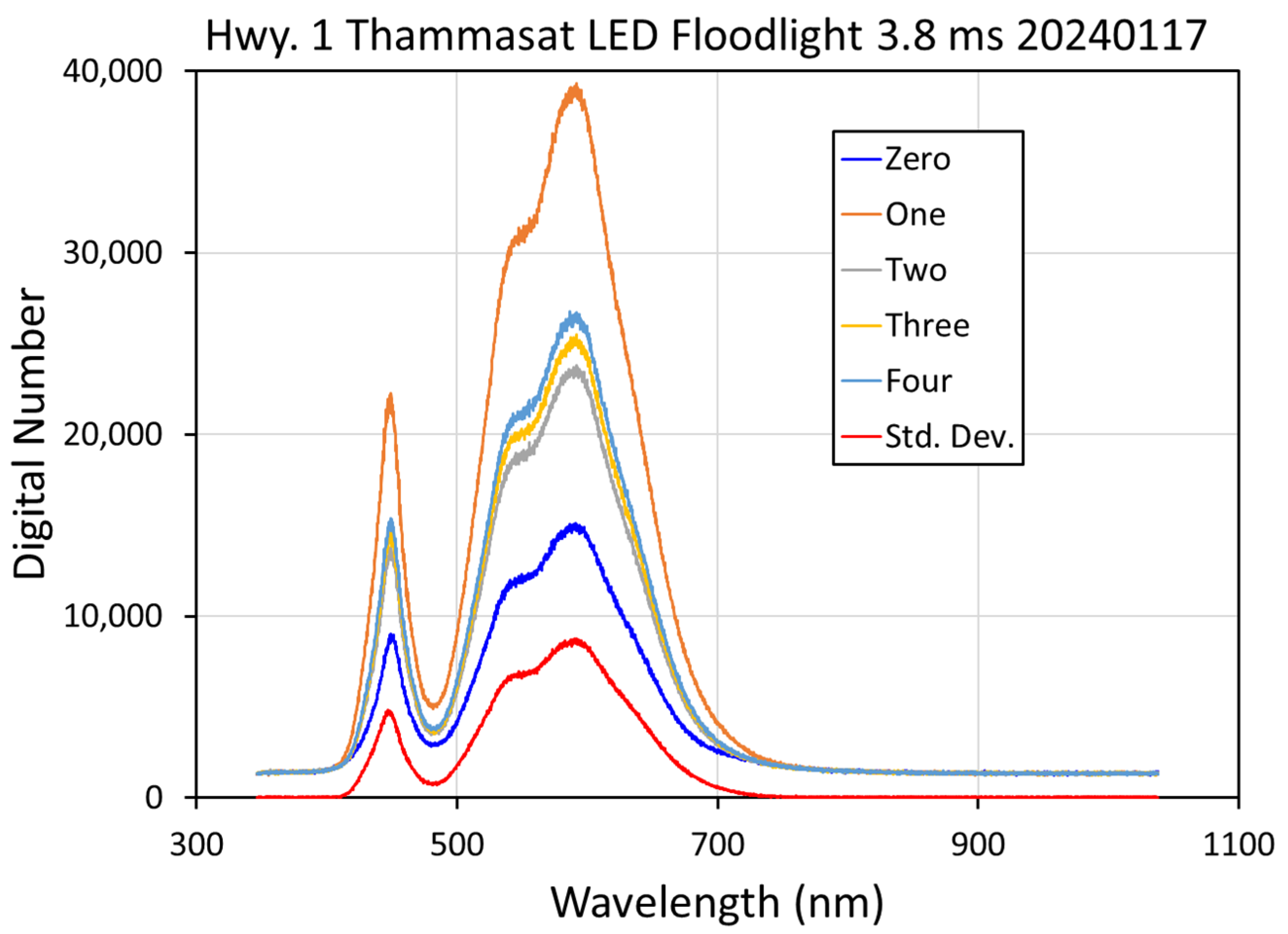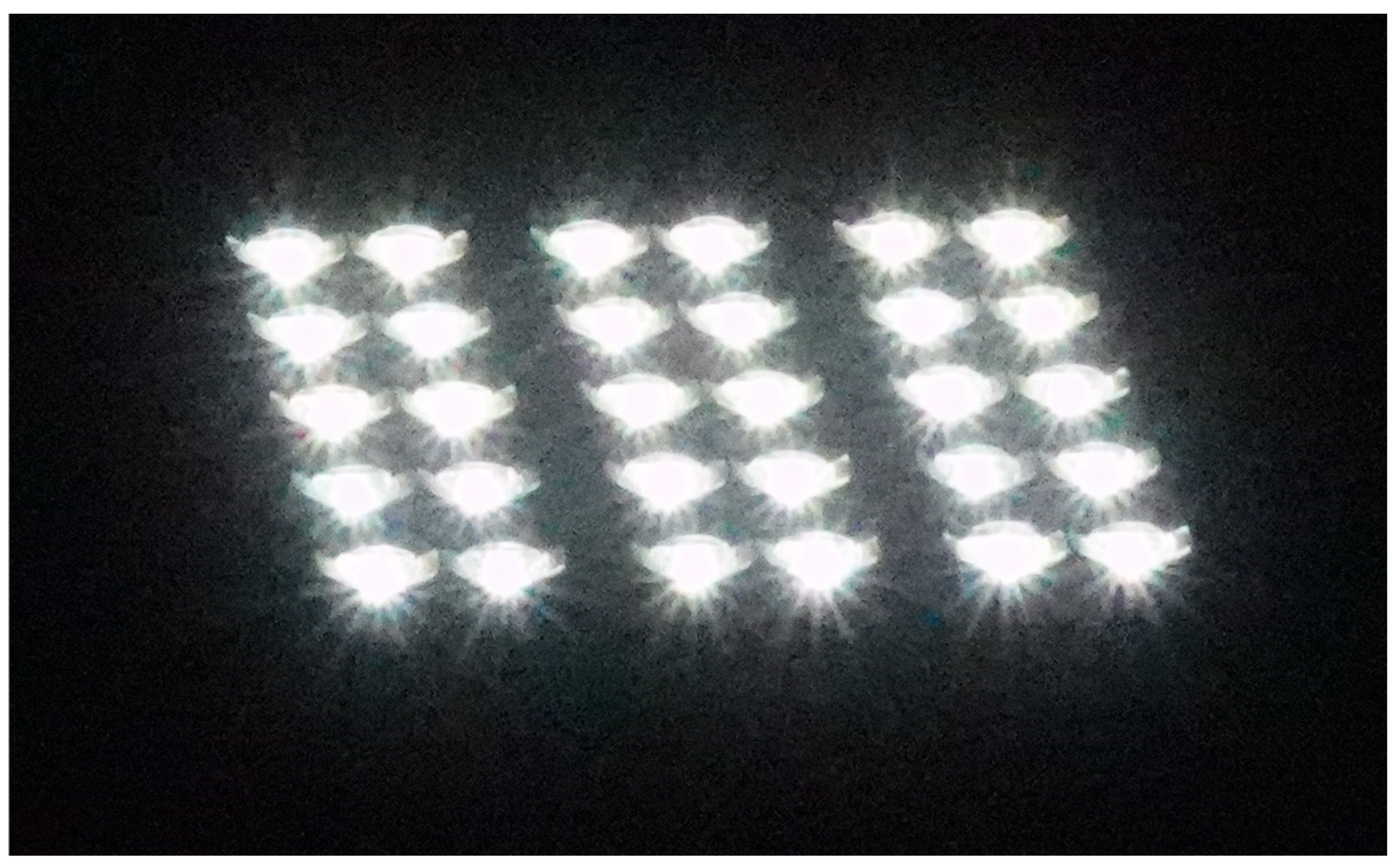The first light to be measured this way is a flickering LED spotlight (Figure 11) used to illuminate the wall sign for Thammasat University along Highway 1, north of Bangkok. A second collection was made on a flickering metal halide lighting cluster on a tall pole at the Heritage Park sport fields in Henderson, Nevada.

The 3.8 ms integration time is 45.6% of the 120 Hz flicker cycling from the two light sources. The Thammasat University LED spotlight is composed of three eight by nine LED arrays (Figure 11). This LED has a high percent flicker, and the flickering of the individual LEDs is fully synchronized. This results in 3.8 ms spectra that rise and fall, changing from one spectrum to the next (Figure 12). The Heritage Park tall pole metal halides are actually bundles of metal halide luminaires with at least two synchronization phases (Figure 8, Figure 9 and Figure 10). The individual spectra are largely steady, but the amplitude of several of the line emissions varies (Figure 13), probably due to the lack of synchronization of the individual luminaires within the assemblage.

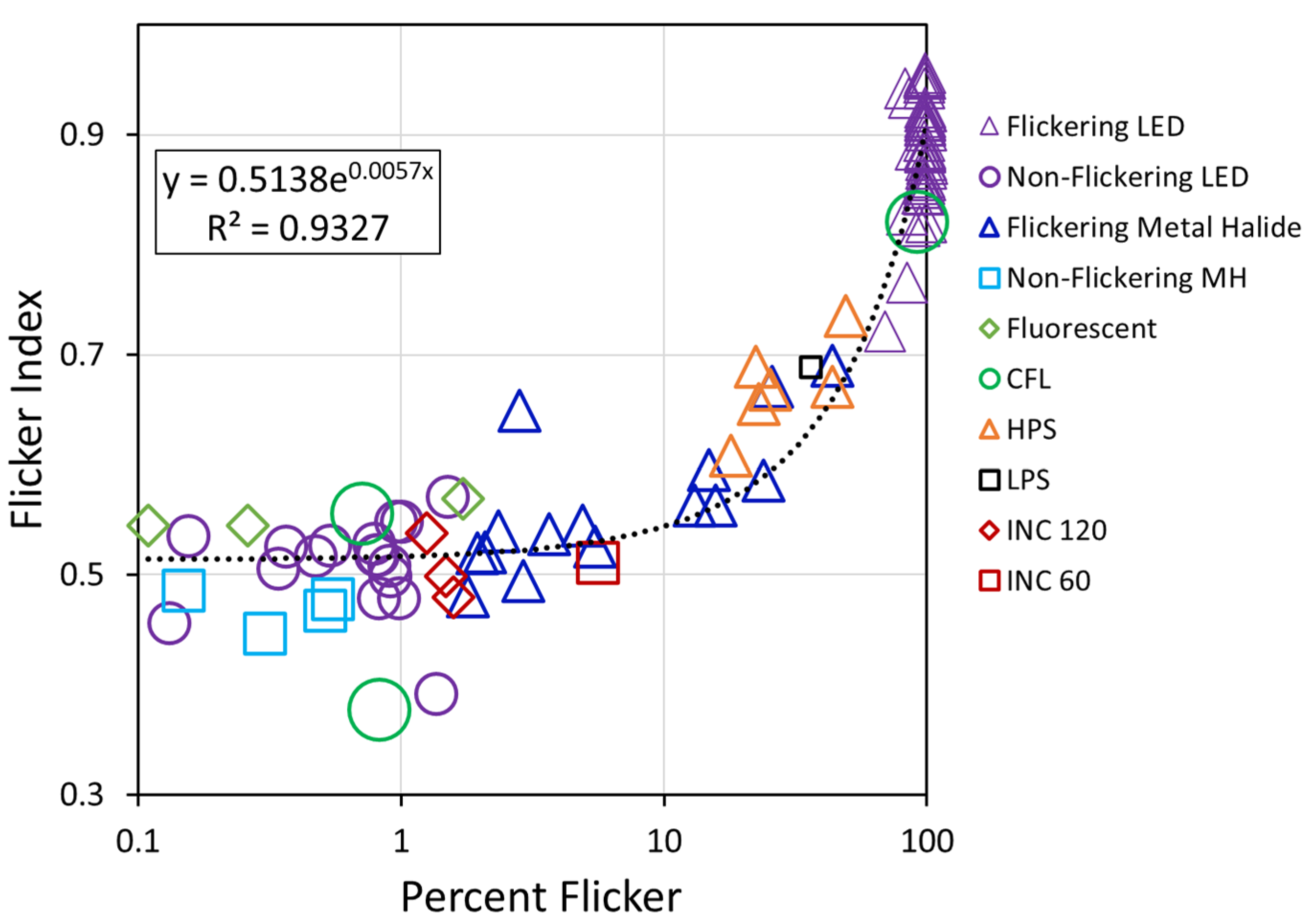
4.11. Summary of Percent Flicker and Flicker Index Values

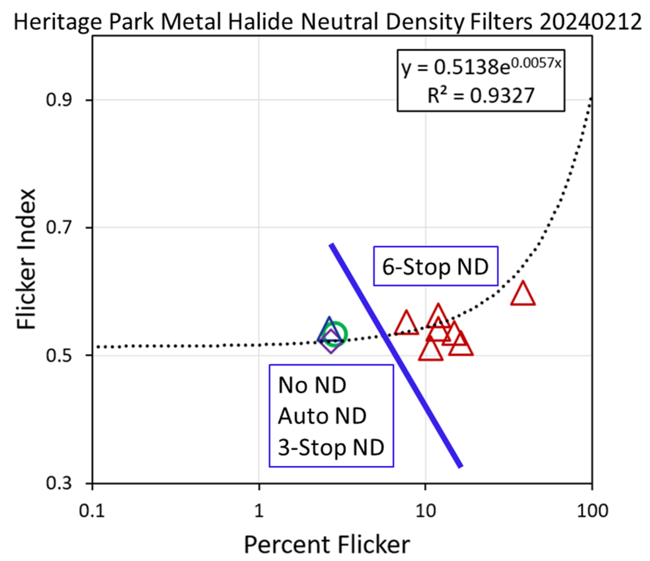
The percent flicker and flicker index values were calculated for each of the measured artificial lights. The results for the collection made without a neutral density filter are plotted in Figure 14. The two indices are highly correlated in an exponential manner. Based on these results, we place the demarcation between flickering and non-flickering at 1% flicker. The results for the neutral density filter collections are shown in Figure 15. The no-ND filter, automatic ND, and three-stop ND indices are locked together with percent flicker near 2.74% and flicker indices near 0.532. In the six-stop neutral density filter data, the saturation effects are gone, leading to an increase in percent flicker.

5. Discussion

5.1. Advantages of High-Speed Cameras over Flickermeters

High-speed cameras have four key advantages over flickermeters. The first of these is the ability to collect flicker data on large numbers of luminaires simultaneously. This makes it possible to analyze the synchronization of flicker and phase shifts that lead to destructive interference. Second, flicker data can be collected for luminaires from several meters to 1–2 km away from the camera position. Third, it is possible to identify flickering versus non-flickering luminaires and clusters of luminaires with synchronized flicker in real time, thus improving the planning of additional collections. Fourth, the cameras can produce scene-wide averages, which cannot be collected by flickermeters.

5.2. Disadvantages

There are at least three disadvantages of high-speed cameras versus flickermeters. First, collections are subject to the effects of saturation, which dampens the flicker in temporal profiles. Switching the camera to a neutral density filter mode will reduce the saturation of bright lights, but dim lights may drop below the camera’s detection limits. Second, post-processing steps are required to extract temporal profiles for quantitative analysis. Third, temporal profiles for collections on distant luminaries can be unstable and not fully usable.

5.3. How Identify Flickering versus Non-Flickering Lights in Real Time

The Sony camera has two periods where the flickering state of luminaires can be identified in real time. The first opportunity to do this is when the camera is in high-frame-rate (HFR) standby mode. Here, the camera is ready to collect at one thousand frames per second, and the flicker state can be observed using the image screen on the back of the camera. In standby mode, it is possible to move the camera to survey the surroundings for flicker, which is useful for planning data collections. The second opportunity for the real-time detection of flickering is the record mode, when the MP4 is played back in slow motion on the camera’s image screen. The record phase lasts 2.5 min.

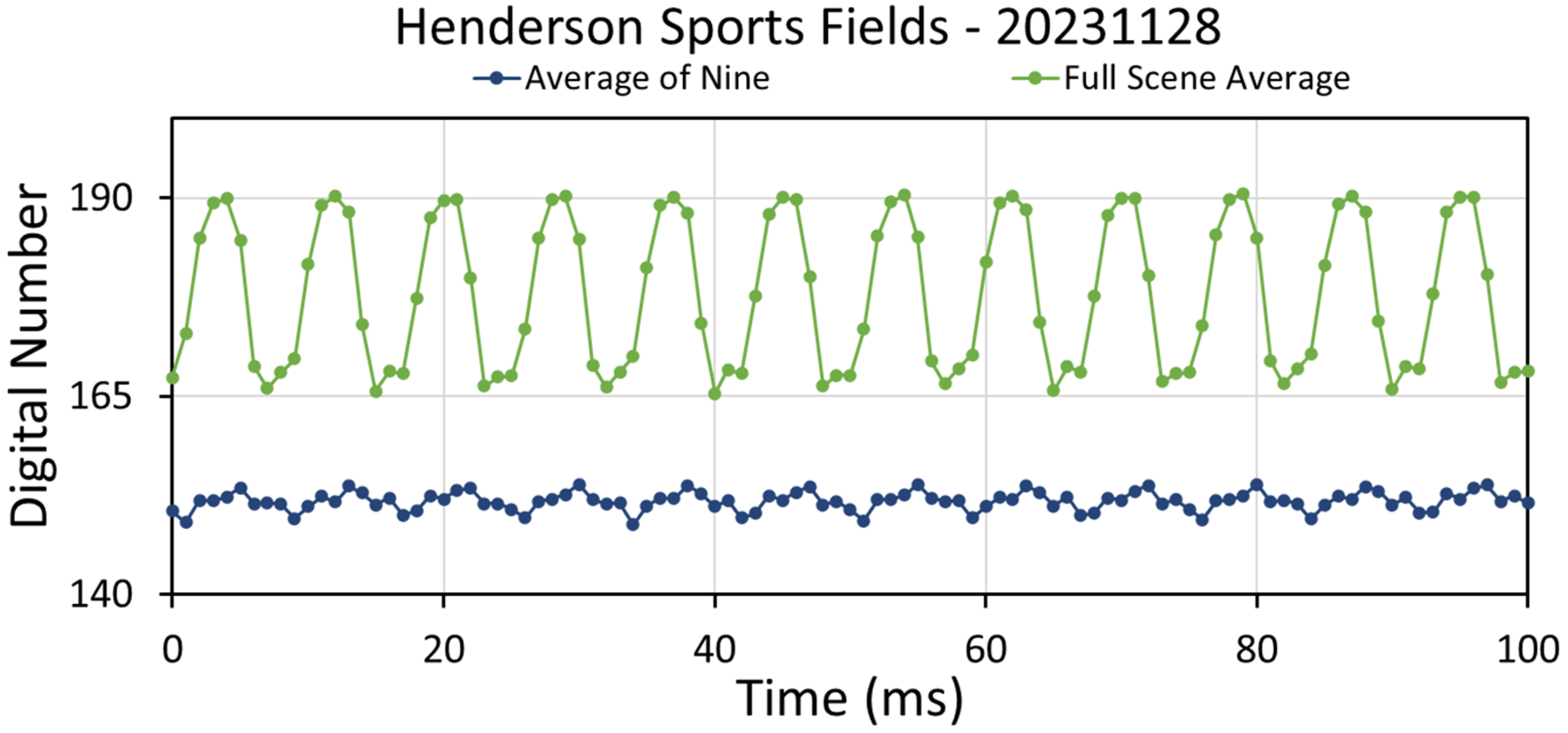
5.4. Recognizing Partial Destructive Interference in Full Scene Temporal Profiles

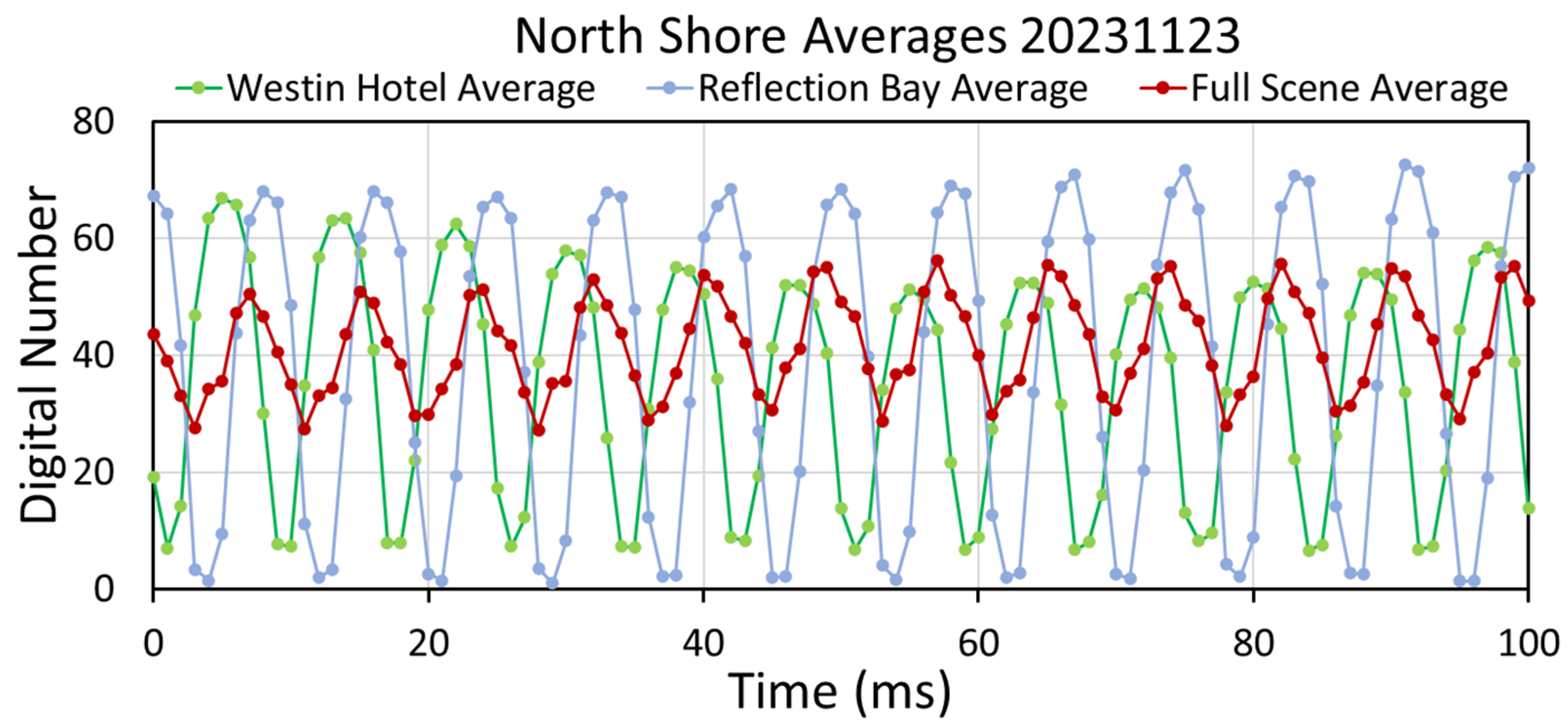
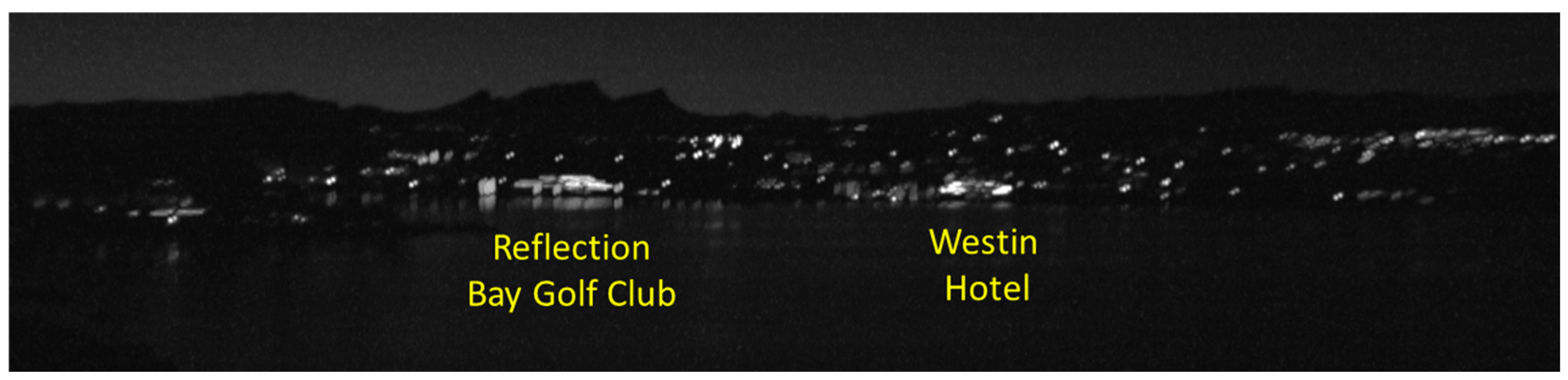
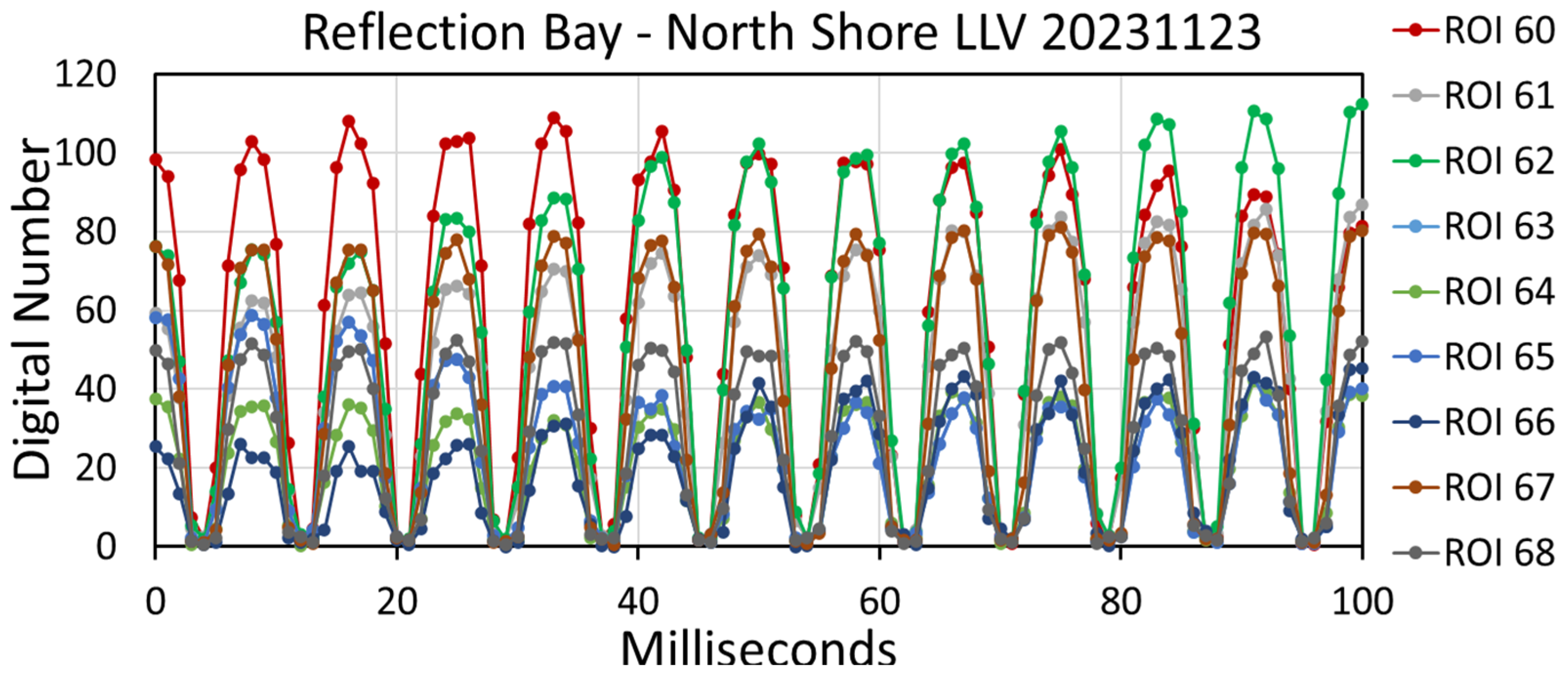
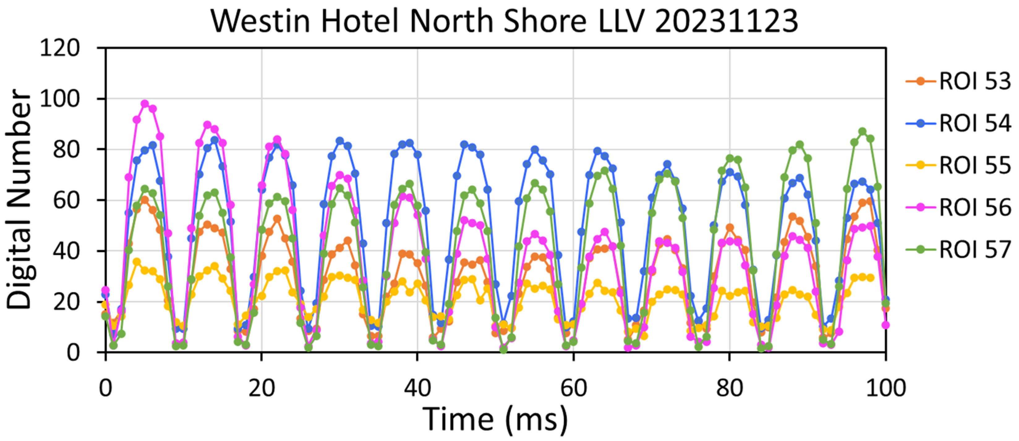
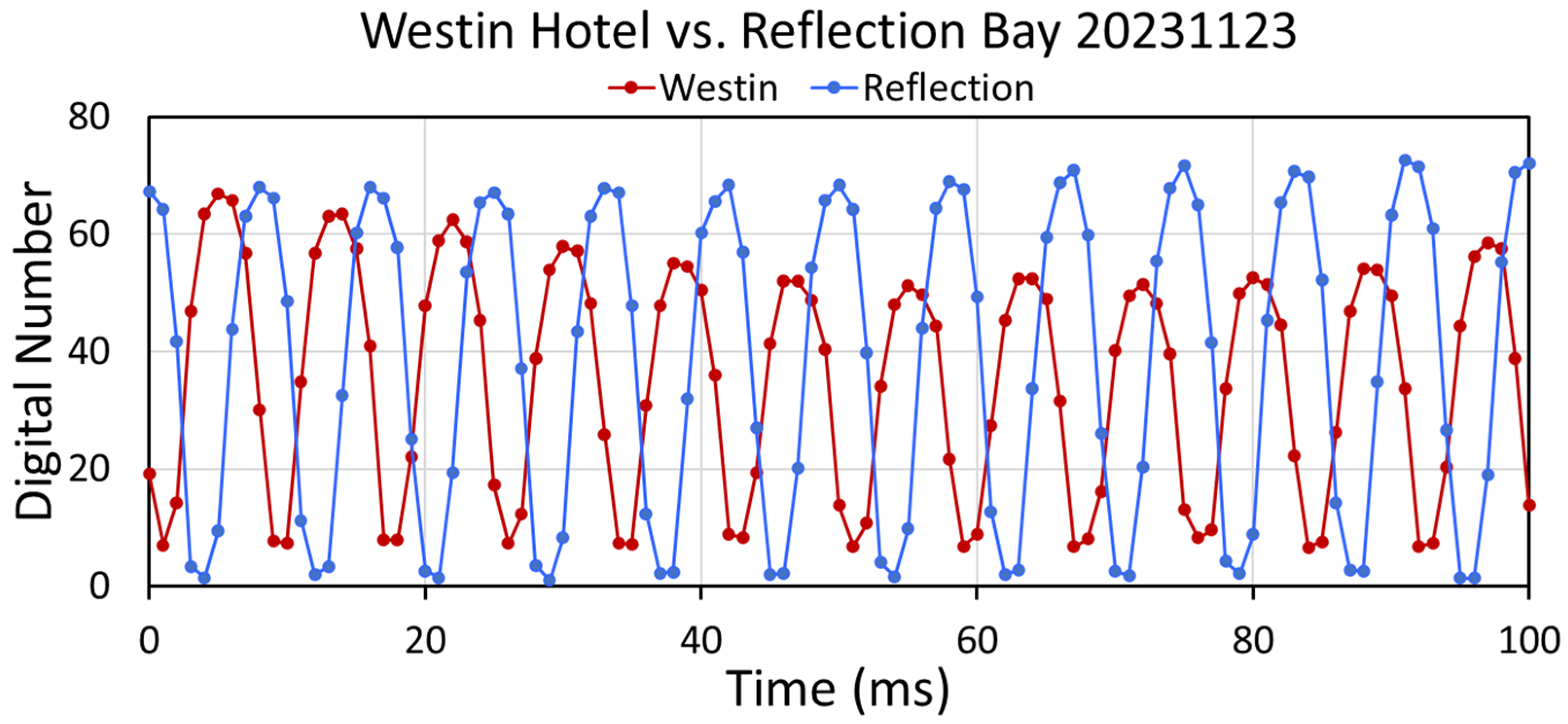
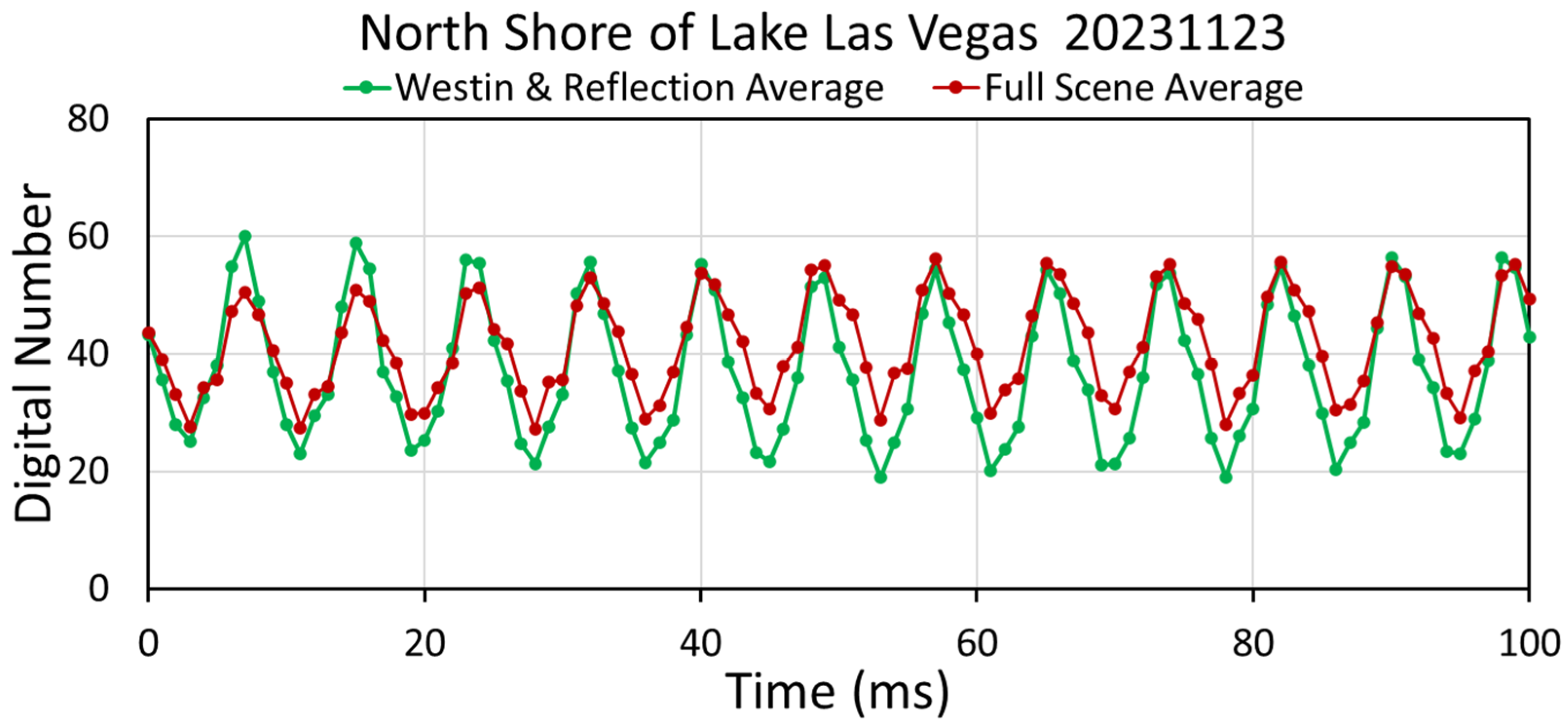
If all the luminaires in a scene are flickering in synchronization, the flicker will be expressed well in the full-scene temporal profile. We found that the flicker is frequently synchronized at the level of individual homes or facilities and for strings of streetlights having shared power supplies. The full-scene averages provide simulations of the flicker level observed by satellite sensors, such as VIIRS. If there are phase differences in the flickering of luminaires within a scene, destructive inference dampens the scene’s average flicker. In some cases, this results in the complete loss of flickering at the full-scene level. However, in many cases, the flicker is still detectable, but the shape of the profile is affected through the interplay of multiple flicker sources having partial synchronization. An example of this is found in the North Shore flicker profiles, where the full-scene temporal profile has a sawtooth pattern (Figure 16). In each flicker cycle, there are two places where the Westin and Reflection Bay lines cross. These crossover points are near the peak and trough of the full-scene average. A sawtooth pattern in full-scene average temporal profiles is an indicator of the partial destructive interference of the various flickering sources present.

5.5. Can Surface Reflectance Result in Exposure to Flicker?

One of the key findings of our study is that bright flickering lights can be reflected by the surrounding Earth’s surface (Figure A39). Surface reflectance provides an additional source of exposure to flicker. Thus, there are three mechanisms for exposure to flicker: (1) via the direct viewing of flickering lights; (2) by viewing of the glow surrounding a flickering light; and (3) via the reflectance of flickering lights off the Earth’s surface. The exposure to surface-reflected flicker can be substantial for organisms who focus their vision on the Earth’s surface. The presence of flicker from surfaces surrounding flickering lights was discovered at the Henderson playing field, where saturation dampened the flicker in the temporal profiles of the tall pole lights, but the scene average showed a well-developed flicker reflecting off of the playing field closest to the camera.

5.6. Recognizing Spurious Temporal Profiles

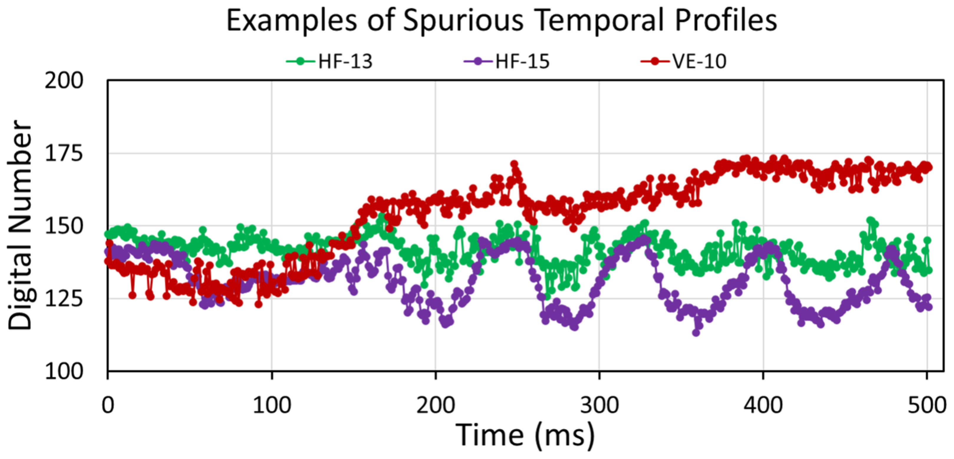
It is not uncommon to find spurious temporal profiles in the collected MP4 datasets. The percentage of these appears to be linked to the distance away from the camera. Factors that may contribute to the spurious profiles include wind, atmospheric turbulence, obstruction by trees, or waves. Figure 17 shows three examples of spurious profiles, one from the Villa Elizabeth and two from the Henderson playing fields. The data user may decide to exclude the spurious profiles from quantitative analysis. Note that the 11 Hz cycling extends beyond 200 ms in the two Henderson sport field spurious temporal profiles. The 11 Hz cycling is real and matches the slow visual swirling of the bright white orb surrounding each the tall pole lights. This phenomenon deserves additional investigation, as an 11 Hz flicker is below the critical fusion frequency for most organisms.

5.7. Why Do Flickering LEDs Have the Highest Percent Flicker?

Incandescent, metal halide, and high-pressure sodium luminaires all have high operating temperatures, above 2000 K (

Table 3. Operating temperatures of common types of outdoor lighting.

Type	Operating Temperature	Reference
High-pressure Sodium	3600–4100 K	[47]
Metal Halide	3300–3400 K	[46]
Incandescent	2500–3000 K	[48]
Fluorescent	300–700 K	[49]
LED	313–328 K	[50]

). For these devices producing light via heat, thermal inertia dampens the amplitude of the flicker and, hence, lowers the percent flicker. The voltage drop in flicker cycling is too short for the bulb to cool substantially, which dampens the dimming during the trough portion of the flickering cycles. LEDs operate in the range from 313 to 328 K—near ambient temperatures. Since the LED light is not producing light via high temperature, the brightness drops quite far during the trough phase of voltage cycling. This thermal inertia effect on the amplitude of flicker was described in a technical report from the International Commission on Illumination (CIE) [37]. Here is a quote from the CIE on the thermal inertia phenomena in different types of luminaires: “The fast reaction of solid-state light sources is in sharp contrast to the reaction times of previous generations of electric light sources. Incandescent and halogen sources have emissions based on thermal processes that are slower than electrical processes. This is evident in the so-called “afterglow” effect of an incandescent lamp being switched off.” Regarding high-intensity discharge lamps the CIE [37] states that “metal halide lamps are well known for their inability with respect to temporal modulation. Many of them need more than 30 min after switching off before they can be switched on again”.

5.8. How Do Lighting Manufacturers Eliminate Flicker in Their Devices?

Non-flickering LEDs have built-in digital drivers that smooth the voltage on its way to the LED. In addition, the coatings placed on top of LED lights in some cases have been cured to reduce flicker. Prior to the development of these methods by manufacturers, there were several influential publications on the LED flicker problem [49,51]. Other papers explored methods to reduce or eliminate flicker in LED lights [52,53,54,55]. It appears that high-end LED manufacturers put in considerable effort to eliminate flicker in the devices they sell. A similar process likely occurred for fluorescent lights.

5.9. Best Not to Guess the Flicker Status of a Light without Measuring It

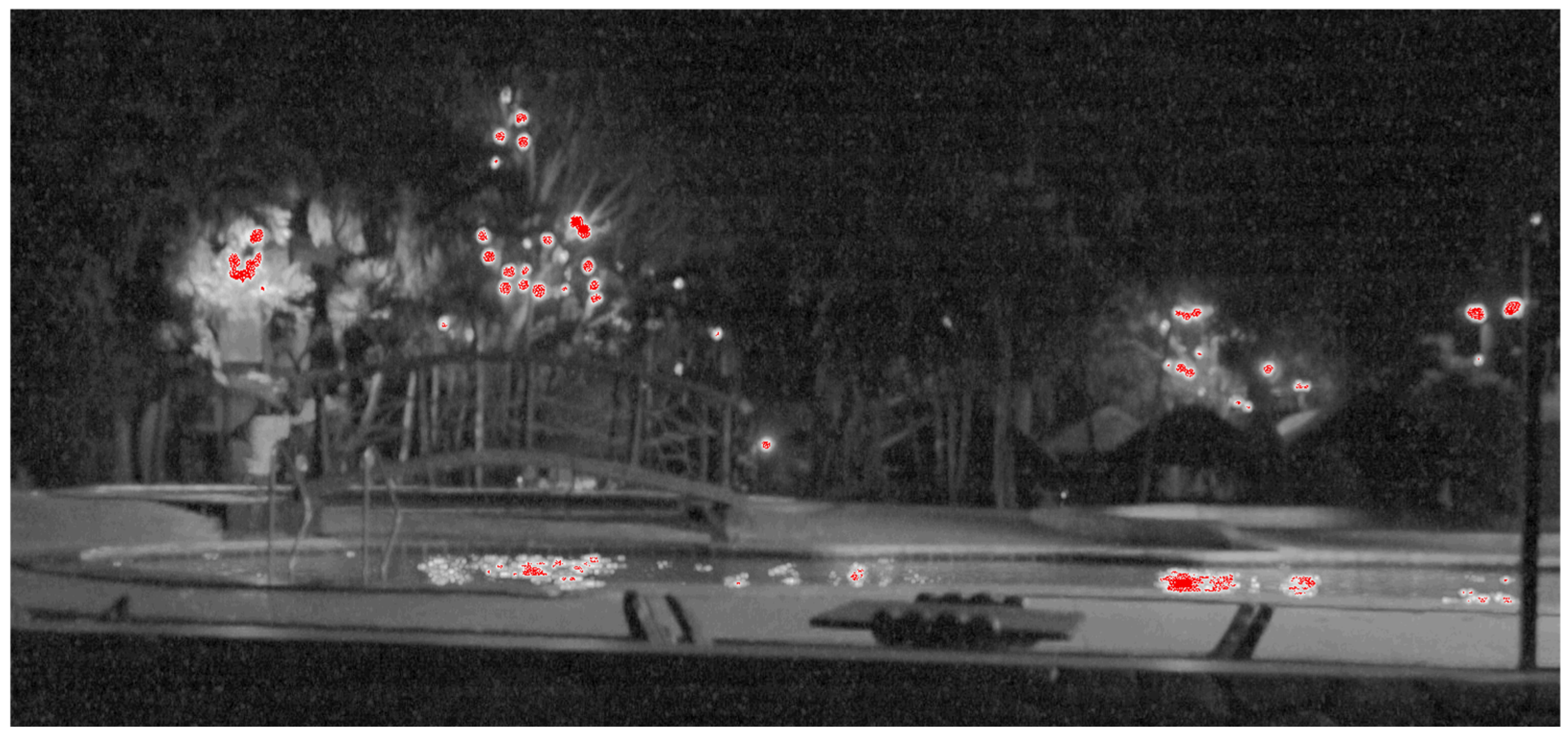
There is a saying that “you can never judge a book by its cover”. This concept is true for the determination of whether a particular artificial light has flicker or not. In our 2021 Flickerfest measurements with a high-speed camera [20], we found that none of the four LED streetlights had flicker above 1% (Table 2), while all four of the metal halide lamps had flicker above 13%. It was not until the current second round of measurements in 2023 that we found LED lights with flicker and metal halide streetlights lacking flicker. While the LED streetlights we measured in 2023 had near-zero flicker, smaller LED devices that we measured commonly had flicker. We even found a population of small LED lights at the Villa Elizabeth where flickering and non-flickering LED lights coexisted. So, it is best to measure the flicker and not make any assumptions based on previous samples measured. The identification of flickering versus non-flickering lights can be determined in the field during the Sony camera’s slow-motion MP4 playback during the recording phase of the data collection.

6. Conclusions

Lighting flicker continues to be widespread around the world. There is substantial evidence that lighting flicker is an endocrine disruptor, similar to blue light. Most studies on the impact of artificial lighting on organisms do not include the measurement of flicker in their experimental designs and focus only on the spectral characteristics of lights and their brightness level. Lighting effects on organisms can arise in response to five aspects of artificial lighting: the time of day, the duration of the exposure, the spectral distribution, the brightness, and the flicker state. To properly attribute the response of organisms to artificial light, each of these aspects must be varied and measured. A good way to design an experiment to determine the impacts of flicker on organisms is by using identical lights—one set with flicker and another set with no flicker. Insects and birds are particularly susceptible to lighting flicker due to their high critical fusion frequencies (Table 1).

Our analysis of percent flicker and the flicker index found that the two are related logarithmically. As the percent flicker reaches the highest levels (above 80%), the flicker index also reaches its highest state, above 0.8. Even lights with no obvious flicker can continue to have flicker detected in the autocorrelation function and percent flicker. We set the threshold for flickering light to 1% flicker.

Flickering and non-flickering varieties of luminaires have been developed for several lighting types, including LED, metal halide, fluorescent, and compact fluorescent lights. LED luminaires are prone to high percent flicker due to their operation near ambient temperatures. Percent flicker is much lower in luminaires that operate at high temperatures such as incandescent, metal halide, and high-pressure sodium. Thermal inertia in luminaires that rely on high temperatures results in a dampening of the percent flicker as the time span of the voltage trough is small compared to the time required for the light to cease radiant emission.

It appears that the high percent flicker of early LED luminaires [49,51] spurred manufacturers to develop LED lights that are free of flicker. This has been achieved through the implementation of built-in digital drivers to smooth AC cycling and through the use of slow-decay phosphor coatings [52,53,54,55].

One of the new findings from our study is that some offshore vessels have flickering lights. Thousands of boats worldwide use strings of metal halide lights above ship decks to attract sea life at night. This is an additional source of exposure to light pollution for sea life, birds, and insects.

Another new finding is that exposure to lighting flicker can come from light reflected from the Earth’s surfaces. This was found at the Henderson playing fields but was also noticed in the Villa Elizabeth and Tayabas Bay MP4 collections. This can be a substantial source of flicker exposure for organisms who tend to keep their eyes on the surrounding Earth’s surface.

High-speed cameras are particularly useful for the identification of flicker luminaires on a landscape scale. We successfully collected usable temporal profiles for light that was placed 1–2 km from the camera. However, when the lights are farther away, the occurrence of spurious temporal profiles is more frequent, resulting in unstable brightness levels. The source of the instability may be wind, atmospheric turbulence, obstruction by vegetation, or the destructive inference of unsynchronized lighting sources. Spurious profiles can be omitted from the dataset used for the quantitative analysis of flicker.

We found several spurious temporal profiles at the Henderson playing fields that have 11 Hz flickering. These profiles will need additional measurements and investigation to determine the source of low Hz flickering.

Lighting synchronization is an important variable to assess in terms of the satellite remote sensing of flicker. The high-speed camera is particularly well suited for identifying synchronized flickering. This has relevance to the satellite detection of flickering. The VIIRS DNB can detect dim lighting down to 1000 watts on the ground and has 742 × 742 meter pixel footprints. While the repeat cycle of VIIRS does not permit the direct detection of flickering cycles, the dwell time of 2–3 ms is in a range where the recorded radiances could fluctuate over time if flicker is synchronized. The effect of flicker is to increase the variance in DNB temporal profiles. A recent study [20] found that the conversion from flickering HPS streetlights to non-flickering LED resulted in a decrease in variance in the DNB temporal profile [20]. What we found in this study is that lighting flickers are often synchronized at the site level. For instance, we found that lighting flickers are synchronized at both the Westin Hotel and Reflection Bay Golf Club on the North Shore of Lake Las Vegas, Nevada. However, the flickers at the two sites are out of phase by about a quarter cycle. This results in some decay in the amplitude of flicker from the full-scene temporal profile. However, the flicker persists even at the full-scene level. The partial destructive inference resulted in a sawtooth temporal profile with 120 Hz cycling.

Another issue we found with the high-speed camera was saturation. The Sony camera collects data in byte format, with a digital number range of 0 to 255. The maximum of 255 indicates that the light has reached saturation. We identified saturated pixels with the maximum DN in composite images produced by the MP4 processing algorithm by color coding the 255 DN pixels with a specific color. Many of the 2023 collections had some level of saturation. Saturation dampens the flicker peaks and, thus, acts to lower the percent flicker and flicker index. Experiments with neutral density filters show that it is possible to reduce or eliminate saturation. High speed camera data collected through low transmissivity neutral density filters results in the loss of detection from dimmer luminaires in the MP4. So, if the dimmer luminaires are of interest, collections can be made with and without a neutral density filter. Data collections with saturation can be used to identify flickering lights, but the flicker amplitude will be dampened.

In conclusion, high-speed cameras provide a valuable method for expanding the study of flickering luminaires. These cameras may enable the inclusion of flicker state in future studies on the impact of artificial lighting on organisms.

References

1. Kyba, C.C.M.; Mohar, A.; Posch, T. How bright is moonlight? Astron. Geophys. 2017, 58, 1.31–1.32. [Google Scholar] [CrossRef]
2. Augustin, A.J. The physiology of scotopic vision, contrast vision, color vision, and circadian rhythmicity: Can these parameters be influenced by blue-light-filter lenses? Retina 2008, 28, 1179–1187. [Google Scholar] [CrossRef] [PubMed]
3. Gowlett, J.A.J. The discovery of fire by humans: A long and convoluted process. Philos. Trans. R. Soc. B Biol. Sci. 2016, 371, 20150164. [Google Scholar] [CrossRef] [PubMed]
4. Weisbuch, C. Historical perspective on the physics of artificial lighting. Comptes Rendus Phys. 2018, 19, 89–112. [Google Scholar] [CrossRef]
5. National Candle Association. Available online: https://candles.org/history/ (accessed on 19 December 2023).
6. Burgin, R. The development of tungsten filament lamps. Light. Res. Technol. 1984, 16, 61–72. [Google Scholar] [CrossRef]
7. Lossev, O.V. CII. Luminous carborundum detector and detection effect and oscillations with crystals. Lond. Ed-Inburgh Dublin Philos. Mag. J. Sci. 1928, 6, 1024–1044. [Google Scholar] [CrossRef]
8. International Energy Agency. Available online: https://www.iea.org/energy-system/buildings/lighting (accessed on 19 December 2023).
9. Kyba, C.C.; Kuester, T.; Sánchez de Miguel, A.; Baugh, K.; Jechow, A.; Hölker, F.; Bennie, J.; Elvidge, C.D.; Gaston, K.J.; Guanter, L. Artificially lit surface of Earth at night increasing in radiance and extent. Sci. Adv. 2017, 3, e1701528. [Google Scholar] [CrossRef] [PubMed]
10. Russart, K.L.; Nelson, R.J. Light at night as an environmental endocrine disruptor. Physiol. Behav. 2018, 190, 82–89. [Google Scholar] [CrossRef] [PubMed]
11. Rich, C.; Longcore, T. (Eds.) Ecological Consequences of Artificial Night Lighting; Island Press: Washington, DC, USA, 2013. [Google Scholar]
12. Lafitte, A.; Sordello, R.; Legrand, M.; Nicolas, V.; Obein, G.; Reyjol, Y. Does a flashing artificial light have more or conversely less impacts on animals than a continuous one? A systematic review. Nat. Conserv. 2023, 54, 149–177. [Google Scholar] [CrossRef]
13. Seymoure, B.M.; Linares, C.; White, J. Connecting spectral radiometry of anthropogenic light sources to the visual ecology of organisms. J. Zool. 2019, 308, 93–110. [Google Scholar] [CrossRef]
14. Cougnard-Gregoire, A.; Merle, B.M.J.; Aslam, T.; Seddon, J.M.; Aknin, I.; Klaver, C.C.W.; Garhöfer, G.; Layana, A.G.; Minnella, A.M.; Silva, R.; et al. Blue Light Exposure: Ocular Hazards and Prevention—A Narrative Review. Ophthalmol. Ther. 2023, 12, 755–788. [Google Scholar] [CrossRef] [PubMed]
15. Chaves, I.; Pokorny, R.; Byrdin, M.; Hoang, N.; Ritz, T.; Brettel, K.; Essen, L.O.; Van Der Horst, G.T.; Batschauer, A.; Ahmad, M. The cryptochromes: Blue light photoreceptors in plants and animals. Annu. Rev. Plant Biol. 2011, 62, 335–364. [Google Scholar] [CrossRef] [PubMed]
16. Wahl, S.; Engelhardt, M.; Schaupp, P.; Lappe, C.; Ivanov, I.V. The inner clock—Blue light sets the human rhythm. J. Biophotonics 2019, 12, e201900102. [Google Scholar] [CrossRef]
17. Hatori, M.; Gronfier, C.; Van Gelder, R.N.; Bernstein, P.S.; Carreras, J.; Panda, S.; Marks, F.; Sliney, D.; Hunt, C.E.; Hirota, T.; et al. Global rise of potential health hazards caused by blue light-induced circadian disruption in modern aging societies. NPJ Aging Mech. Dis. 2017, 3, 9. [Google Scholar] [CrossRef] [PubMed]
18. Falchi, F.; Cinzano, P.; Elvidge, C.D.; Keith, D.M.; Haim, A. Limiting the impact of light pollution on human health, environment and stellar visibility. J. Environ. Manag. 2011, 92, 2714–2722. [Google Scholar] [CrossRef] [PubMed]
19. Wilkins, A.; Veitch, J.; Lehman, B. LED lighting flicker and potential health concerns: IEEE standard PAR 1789 update. In Proceedings of the 2010 IEEE Energy Conversion Congress and Exposition, Atlanta, GA, USA, 12–16 September 2010; pp. 171–178. [Google Scholar]
20. Elvidge, C.D.; Zhizhin, M.; Keith, D.; Miller, S.D.; Hsu, F.C.; Ghosh, T.; Anderson, S.J.; Monrad, C.K.; Bazilian, M.; Taneja, J.; et al. The VIIRS Day/Night Band: A Flicker Meter in Space? Remote Sens. 2022, 14, 1316. [Google Scholar] [CrossRef]
21. Shady, S.; MacLeod, D.I.A.; Heidi, S.F. Adaptation from invisible flicker. Proc. Natl. Acad. Sci. USA 2004, 101, 5170–5173. [Google Scholar] [CrossRef]
22. Mander, S.; Alam, F.; Lovreglio, R.; Ooi, M. How to measure light pollution—A systematic review of methods and applications. Sustain. Cities Soc. 2023, 92, 104465. [Google Scholar] [CrossRef]
23. Gokus, A.; Hänel, A.; Ruby, A.; Dröge-Rothaar, A.; Küchly, B.; Kyba, C.C.; Fischer, D.; Gruber, D.; Weiß, E.C.; Klan, F.; et al. The Nachtlichter App: A citizen science tool for documenting outdoor light sources in public spaces. Int. J. Sustain. Light. 2023, 25, 24–66. [Google Scholar] [CrossRef]
24. Drapela, J.; Slezingr, J. Design and utilization of a light flickermeter. In Proceedings of the 2012 IEEE International Workshop on Applied Measurements for Power Systems (AMPS) Proceedings, Aachen, Germany, 26–28 September 2012; pp. 1–6. [Google Scholar]
25. Inger, R.; Bennie, J.; Davies, T.W.; Gaston, K.J. Potential biological and ecological effects of flickering artificial light. PLoS ONE 2014, 9, e98631. [Google Scholar] [CrossRef]
26. Mankowska, N.D.; Marcinkowska, A.B.; Waskow, M.; Sharma, R.I.; Kot, J.; Winklewski, P.J. Critical flicker fusion frequency: A narrative review. Medicina 2021, 57, 1096. [Google Scholar] [CrossRef] [PubMed]
27. Gautam, D.; Vinay, D. A Study of Critical Flicker Fusion Threshold among Smartphone Users. Int. J. Curr. Microbiol. Appl. Sci. 2020, 9, 2381–2386. [Google Scholar] [CrossRef]
28. Lafitte, A.; Sordello, R.; Legrand, M.; Nicolas, V.; Obein, G.; Reyjol, Y. A flashing light may not be that flashy: A systematic review on critical fusion frequencies. PLoS ONE 2022, 17, e0279718. [Google Scholar] [CrossRef] [PubMed]
29. Berman, S.M.; Greenhouse, D.S.; Bailey, I.L.; Clear, R.D.; Raasch, T.W. Human electroretinogram responses to video displays, fluorescent lighting and other high frequency sources. Optom. Vis. Sci. 1991, 68, 645–662. [Google Scholar] [CrossRef]
30. Davis, J.; Hsieh, Y.-H.; Lee, H.-C. Humans perceive flicker artifacts at 500 Hz. Sci. Rep. 2015, 5, 78. [Google Scholar] [CrossRef]
31. Wilkins, A.J. Health and efficiency in lighting practice. Energy 1993, 18, 123–129. [Google Scholar] [CrossRef]
32. Price, L.L.A. Can the Adverse Health Effects of Flicker from LEDs and Other Artificial Lighting Be Prevented? Leukos 2017, 13, 191–200. [Google Scholar] [CrossRef]
33. Boyce, P.R. Light, lighting and human health. Light. Res. Technol. 2022, 54, 101–144. [Google Scholar] [CrossRef]
34. Kozaki, T.; Hidaka, Y.; Takakura, J.-Y.; Kusano, Y. Salivary melatonin suppression under 100-Hz flickering blue light and non-flickering blue light conditions. Neurosci. Lett. 2020, 722, 134857. [Google Scholar] [CrossRef]
35. Illuminating Engineering Society. Percent Flicker. Available online: https://www.ies.org/definitions/percent-flicker/ (accessed on 1 January 2024).
36. Illuminating Engineering Society. Flicker Index. Available online: https://www.ies.org/definitions/flicker-index/ (accessed on 1 January 2024).
37. International Illumination Commission (CIE). Visual Aspects of Time-Modulated Lighting Systems—Definitions and Measurement Models; Technical Note; CIE TN 006:2016; CIE: Vienna, Austria, 2016; pp. 1–23. [Google Scholar]
38. Perz, M.; Vogels, I.M.L.C.; Sekulovski, D.; Wang, L.; Tu, Y.; Heynderickx, I.E.J. Modeling the visibility of the stroboscopic effect occurring in temporally modulated light systems. Light. Res. Technol. 2015, 47, 281–300. [Google Scholar] [CrossRef]
39. Klej, A.; Beeckman, P.; Mila, N.; Banerjee, K.; Embrechts, M. Flicker (pstLM) and stroboscopic effect (SVM)–light measurements in photometrical laboratories. Signify developed setup and validation method. In Proceedings of the 29th Quadrennial Session of the CIE, Washington, DC, USA, 14–22 June 2019; pp. 14–22. [Google Scholar]
40. Petrinska, I.; Ivanov, D. Estimation of flicker of contemporary LED lamps and luminaires. In Proceedings of the 2019 11th Electrical Engineering Faculty Conference (BulEF), Varna, Bulgaria, 11–14 September 2019; pp. 1–4. [Google Scholar]
41. Elvidge, C.D.; Hsu, F.-C.; Zhizhin, M.; Ghosh, T.; Taneja, J.; Bazilian, M. Indicators of electric power instability from satellite observed nighttime lights. Remote Sens. 2020, 12, 3194. [Google Scholar] [CrossRef]
42. Román, M.O.; Wang, Z.; Sun, Q.; Kalb, V.; Miller, S.D.; Molthan, A.; Schultz, L.; Bell, J.; Stokes, E.C.; Pandey, B.; et al. NASA’s Black Marble nighttime lights product suite. Remote Sens. Environ. 2018, 210, 113–143. [Google Scholar] [CrossRef]
43. Berne, B.J.; Boon, J.P.; Rice, S.A.; Berne, B.J.; Boon, J.P.; Rice, S.A. On the calculation of autocorrelation functions of dynamical variables. J. Chem. Phys. 1966, 45, 1086–1096. [Google Scholar] [CrossRef]
44. Elvidge, C.D.; Keith, D.M.; Tuttle, B.T.; Baugh, K.E. Spectral identification of lighting type and character. Sensors 2010, 10, 3961–3988. [Google Scholar] [CrossRef] [PubMed]
45. Wang, S.; Ruan, X.; Yao, K.; Tan, S.-C.; Yang, Y.; Ye, Z. A flicker-free electrolytic capacitor-less AC–DC LED driver. IEEE Trans. Power Electron. 2011, 27, 4540–4548. [Google Scholar] [CrossRef]
46. Fromm, D.C.; Lieder, G.H.; Gleixner, K.H. Gleixner. Investigation of the connection between plasma temperature and electrode temperature in metal-halide lamps. J. Phys. D Appl. Phys. 2002, 35, 1668. [Google Scholar] [CrossRef]
47. De Groot, J.J.; Van Vliet, J.A.J.M. The measurement and calculation of the temperature distribution and the spectrum of high-pressure sodium arcs. J. Phys. D Appl. Phys. 1975, 8, 651. [Google Scholar] [CrossRef]
48. MacIsaac, D.; Kanner, G.; Anderson, G. Basic physics of the incandescent lamp (lightbulb). Phys. Teach. 1999, 37, 520–525. [Google Scholar] [CrossRef]
49. Graeme, G.L.; Waymouth, J.F. Light Sources, In Encyclopedia of Physical Science and Technology, 3rd ed.; Academic Press: Cambridge, MA, USA, 2003. [Google Scholar]
50. Fu, H.-K.; Wang, C.-P.; Chiang, H.-C.; Chen, T.-T.; Chen, C.-L.; Chou, P.-T. Evaluation of temperature distribution of LED module. Microelectron. Reliab. 2013, 53, 554–559. [Google Scholar] [CrossRef]
51. Kitsinelis, S.; Arexis-Boisson, L.; Zhang, Y.; Zissis, G. LED Flicker: A drawback or an opportunity? Opt. Photonics J. 2013, 3, 28940. [Google Scholar] [CrossRef]
52. Tan, J.; Narendran, N. Defining phosphor luminescence property requirements for white AC LED flicker reduction. J. Lumin. 2015, 167, 21–26. [Google Scholar] [CrossRef]
53. Tan, J. Investigation of Solutions to Minimize Flicker in LED Lighting; Rensselaer Polytechnic Institute: New York, NY, USA, 2014. [Google Scholar]
54. Tan, J.; Narendran, N. A driving scheme to reduce AC LED flicker. In LED-Based Illumination Systems; SPIE: Bellingham, WA, USA, 2013; Volume 8835, pp. 156–161. [Google Scholar]
55. Mao, Z.; Ge, L.; Hua, G. Removing the LED light strobe flicker by proper driver designs. In Proceedings of the 2013 10th China International Forum on Solid State Lighting (ChinaSSL), Beijing, China, 10–12 November 2013; pp. 210–213. [Google Scholar]
56. Kazimierczuk, M.K.; Szaraniec, W. Electronic ballast for fluorescent lamps. IEEE Trans. Power Electron. 1993, 8, 386–395. [Google Scholar] [CrossRef]
Figure 1. Flickering versus non-flickering LED temporal profiles.
Atmosphere 15 00438 g001
Figure 2. Spectrum of an LED spotlight for AIT’s wall sign at the Highway 1 campus entrance.
Atmosphere 15 00438 g002
Figure 3. Metal halide spectrum from the Heritage Park sport fields in Henderson, Nevada.
Atmosphere 15 00438 g003
Figure 4. Temporal profiles for flickering and non-flickering metal halide bulbs.
Atmosphere 15 00438 g004
Figure 5. Subsets of the maximum count composite images focused on the lighting clusters on the tall pole closest to the camera. On the left is the maximum count image with a linear contrast stretch. The images on the right show the pixels that reached saturation in the maximum count composite as blue and a red rectangle indicating the sampling area.
Atmosphere 15 00438 g005
Figure 6. Temporal profiles from cluster 0 with no ND filter, automatic ND filtering, and the three-stop ND filter.
Atmosphere 15 00438 g006
Figure 7. With the six-stop ND filter, the MP4 processing software identified seven lighting clusters inside the area where the higher transmissivity collections only found a single saturated lighting feature. Number 9 appears to be a single luminaire. Numbers 6, 7, 8, 10, and 11 appear to have more than one luminaire. Number 5 straddles three lighting clusters.
Atmosphere 15 00438 g007
Figure 8. Three synchronized temporal profiles from the six-stop ND collection.
Atmosphere 15 00438 g008
Figure 9. Temporal profiles for clusters 7 and 9 from the six-stop ND collection. The profile for cluster 8 is added to point out that the flicker amplitudes for 7 and 9 are lower and offset from the cycling seen in Figure 8.
Atmosphere 15 00438 g009
Figure 10. Temporal profiles for clusters 5 and 10 from the six-stop ND collection. Cluster 5 straddles three lights, covering large parts of clusters 6 and 7, plus the light between those two. Since lights 6 and 7 are not synchronized (Figure 8 and Figure 9), it is not surprising the cluster 5’s temporal profiles have the classic sawtooth pattern associated with partial destructive interference, similar to that shown in Figure A14. The temporal profile from cluster 10 is similar to those from the saturated collections shown in Figure 6. Cluster 10’s temporal profile contains a hint of flicker that has been heavily dampened by the presence of multiple unsynchronized lights.
Atmosphere 15 00438 g010
Figure 11. USB4000 spectra were collected with an integration time of 3.8 ms on this outdoor LED spotlight in from of Thammasat University on Highway 1 north of Bangkok.
Atmosphere 15 00438 g011
Figure 12. A set of 3.8 ms integration time spectra of an LED spotlight illuminating the wall sign at the entrance to Thammasat University along Highway 1, north of Bangkok. The standard deviation was calculated from five individual spectra.
Atmosphere 15 00438 g012
Figure 13. USB4000 spectra of a tall pole assemblage of metal halide bulb at the Heritage Park sport fields in Henderson, Navada. The chart shows two temporal profiles and the standard deviation calculated from twelve individual spectra.
Atmosphere 15 00438 g013
Figure 14. Percent flicker versus flicker index values for 92 samples, combining the records from the 2021 Flickerfest and the new collections from 2023.
Atmosphere 15 00438 g014
Figure 15. Percent flicker versus flicker index for the neutral density filter collections on a tall pole lamp metal halide cluster at the Heritage Park sport fields in Henderson, Nevada. The no-ND, auto-ND and three-stop ND index values are locked together due to saturation effects. These are to the left of the blue diagonal line. The six-stop ND data points are located to the right of the blue line, eliminated nearly all of the saturation, making it possible to identify seven individual lighting features with substantially higher percent flicker levels than the saturated observations. The regression line from Figure 14 is repeated here, along with the regression formula. The other two boxes are data labels.
Atmosphere 15 00438 g015
Figure 16. North Shore averages from the Westin Hotel, Reflection Bay, and full scene.
Atmosphere 15 00438 g016
Figure 17. Examples of spurious temporal profiles, which can be excluded from quantitative analysis.
Atmosphere 15 00438 g017