Article

CMIP6 Simulation-Based Daily Surface Air Temperature and Precipitation Projections over the Qinghai-Tibetan Plateau in the 21st Century

1
State Key Laboratory of Simulation and Regulation of Water Cycle in River Basin, China Institute of Water Resources and Hydropower Research, Beijing 100038, China
2
School of Hydraulic and Environmental Engineering, Changsha University of Science and Technology, Changsha 410114, China
*
Author to whom correspondence should be addressed.
Atmosphere 2024, 15(4), 434; https://doi.org/10.3390/atmos15040434
Submission received: 12 February 2024 / Revised: 22 March 2024 / Accepted: 28 March 2024 / Published: 30 March 2024

Abstract

:
The Qinghai-Tibetan Plateau (QTP), the source of many major Asian rivers, is sensitive to climate change, affecting billions of people’s livelihoods across Asia. Here, we developed high-resolution projections of precipitation and daily maximum/minimum temperatures at 0.1° spatial resolution over the QTP. The projections are based on the output from seven global climate models (GCMs) from the Coupled Model Intercomparison Project Phase 6 (CMIP6) for historical (1979–2013) and projected (2015–2100) climates across four scenarios (SSP1-2.6, SSP2-4.5, SSP3-7.0, and SSP5-8.5). An updated nonstationary cumulative distribution function matching method (called CNCDFm) was used to remove model systemic bias. We verify the necessity of taking into account altitude in downscaling processes and the validity of nonstationary bias correction. Compared to the historical period, the climate in the QTP in the 21st century is warmer (1.2–5.1 °C, for maximum surface temperature) and wetter (3.9–26.8%) according to the corrected GCM projection. For precipitation, the Indus River (IDR), Tarim River (TMR), Inner of Qiangtang Basin (IQTB), Yarlung Zangbo (YLZBR), and Qaidam Basin (QDB) showed growth well above the global average across high radiative forcing scenarios, which could have a profound impact on the regional hydrological cycle. However, there is great uncertainty in precipitation prediction, which is demonstrated by a very low signal-to-noise ratio (SNR) and a large difference between Bayesian model averaging (BMA) and multi-model averages (MMAs). This bias-corrected dataset is available for climate change impact research in the QTP at the subregion scale.

1. Introduction

The Qinghai-Tibetan Plateau (QTP), called the Asian Water Tower, is the source of many major Asian rivers, such as the Yellow, Yangtze, Mekong, Indus, Salween, and Brahmaputra [1]. Climate change in the QTP affects billions of people in Asia by changing regional water resources, agricultural production, energy security, and disaster risk [2,3,4,5]. That is why the QTP has attracted the attention of academics and policymakers. In previous studies, the QTP was found sensitive to climate change. Based on historical data and reanalysis data, previous research showed that the QTP area had a more significant increase in temperature than the surrounding areas [6]. However, it is difficult to estimate the spatial distribution of changes in meteorological elements. Because of complex topographic conditions, meteorological factors of the QTP have high spatial heterogeneity, especially in near-surface areas [7,8]. These distribution characteristics may exhibit different evolutionary trends under different climatic backgrounds [9]. Furthermore, low-resolution meteorological data lack representativeness and practical value on the plateau [10].
Numerous downscaling and multi-source data methods have been applied in large-scale regions to provide high-resolution data. In recent years, several high-resolution reanalysis datasets have been evaluated and applied in the Qinghai-Tibetan Plateau (QTP), with precipitation and temperature being the most crucial variables [11,12,13,14,15]. These studies not only demonstrate the possibility of generating high-resolution meteorological data in ungauged regions but also provide forcing data to drive a variety of terrestrial models, which is essential for climatic impact studies [16,17,18]. Nevertheless, due to differences in input data, numerical assimilation models, parameterization schemes, and the spatiotemporal resolutions of final products, these reanalysis datasets exhibit varying performances in different regions [19,20]. Therefore, the question of how to apply the reanalysis data remains worthy of discussion.
Global climate models (GCMs) are effective tools for simulating Earth’s climate on continental scales and larger [21]. They are the most important tools and infrastructure for projecting future climatic conditions and assessing the climate change impact [22]. GCMs have been widely used in climate change research [23,24,25], showing growing potential when used as forcing data for land surface models and hydrological models. The Coupled Model Intercomparison Project Phase 6 (CMIP6) indicates an overall improvement in GCMs over the last decade [22,26]. Typically, the cold bias of CMIP5 on air temperature is significantly reduced in CMIP6 for the QTP [27].
However, major problems still exist and prevent researchers from using GCM results directly. At first, the models in CMIP6 still have considerable systematic biases in meteorological simulation of regional scale. Lun et al. [28] found that the multi-model ensembles (MME) of 23 GCMs in CMIP6 overestimated the QTP precipitation by about 84.1% in historical simulation, and the wet biases of the same models were even higher than historical observation. Secondly, the outputs of GCMs still feature a low resolution that is difficult to align with the input requirements of land and hydrological models, especially when compared to the more detailed scales needed for accurately simulating land and hydrological processes [29]. In general, the resolution of GCM outputs is between 0.5° and 2.5°, which is much larger than most land and hydrological processes. For instance, Su et al. [2] developed a hydrological model to simulate the impact of glacier melt in the QTP, and the model was set up on 0.083° × 0.083° grids because glacier areas are from 100 km2 to 10,000 km2. Hence, downscaling GCMs has become a pre-processing step in many studies, but existing studies tend to use the linear interpolation method in downscaling [2,5,30,31,32], ignoring the influence of the underlying surface on the spatial distribution of climate variables, which may cause further systematic errors. Moreover, GCMs still exhibit large uncertainty that shows up in different models and produces widely different results when they simulate the same variable in the same forcing scenario. In the QTP, Zhang and Yang [27] found that GCM-simulated daily precipitation (including both liquid and solid phases, units: mm d−1) values have large variation, with most values ranging from 1.4 mm d−1 to 3.5 mm d−1. Such large variations make it difficult for users to decide which model is the best model or how to ensemble prediction based on several models. These problems become worse when looking at particular uses of GCM simulation output [22]. But on the other hand, although it is still challenging to obtain optimal projection over the QTP, smaller deviation forecasts (compared to the raw output from CMIP6) based on effective statistical methods are essential for regional-scale studies.
Therefore, this study attempts to produce a 0.1° × 0.1° high-resolution projection over the entire QTP (HRP-QTP) based on reanalysis data and CMIP6 simulations, which includes the historical period (from 1979 to 2013) and future period (from 2015 to 2100), and can be used in watershed scale studies (variables information presented in Table 1). In the present study, combined reanalysis data were applied as historical data for ungauged regions. In order to deal with the complex terrain conditions of the QTP, we adopted a downscaling method different from the linear interpolation commonly used in previous studies to fit the effects of altitude on climate change. Furthermore, an updated bias correction method was used to remove systematic bias from GCM projections. The present study also produced ensemble data from several models. The projection is available for researchers who want to learn about climate change and its impact on the QTP. It also provides a robust and universal method to deal with CMIP6 data, which can be used in other regions confronting climate change risk.

2. Materials and Methods

2.1. Definition and Division of Study Area

As for the scope of the Qinghai-Tibet Plateau, there are different definitions in different studies. We adopted the high-frequency use scope of the QTP (HF-QTP) as defined by Zhang et al. [33], which included several major river headwaters and can match most research requirements. The QTP ranges from 25°59′37″ N to 39°49′33″ N and from 73°29′56″ E to 104°40′20″ E, covering an area of 2542.30 × 103 km2 [34]. Its altitudes range from 85 m to 8233 m, and approximately 90.9% belong to high altitude (>3000 m) areas. This range includes the world’s highest mountains and massive deep valleys in terms of topography. The complex terrain of the QTP results in a complicated distribution of precipitation and surface temperature. A brief overview can be seen in Figure 1. These regions can be divided into ten subregions based on watershed [35,36], as follows: I. Tarim River (TMR); II. Qaidam Basin (QDB); III. Hexi Basin (HXB); IV. Yellow River (YR); V. Inner of Qiangtang Basin (IQTB); VI. Yangtze River (YZR); VII. Indus River (IDR); VIII. Salween River (SWR); IX. Mekong River (MKR); and X. Yarlung Zangbo (YLZBR). Among these, IQTB and QDB belong to the inland river basin, and some of the river channels are seasonal. We obtained the river distribution of QDB from National Basic Geographic Information [37]. Currently, there are only 131 long-observed meteorological stations in the QTP (Figure 1) maintained by the China Meteorological Administration (CMA). They are primarily situated in the eastern part of the QTP, with observations lacking in the western part of the plateau. The digital elevation model (measured from sea level, DEM, units: m) used in this section and Section 2.5 is provided by the National Tibetan Plateau Data Center “https://data.tpdc.ac.cn/ (24 March 2021)” [38].
In Figure 1, the lower Yarlung Zangbo valley (LYZV) is highlighted with red dots. Its boundary is defined by the watershed of lower Yarlung Zangbo and is the joint part of the Yarlung Zangbo River and Brahmaputra River. Unlike other regions in the QTP, LYZV belongs to the south of the Himalayas, is controlled by the Indian monsoon [39,40,41,42,43], and has greatly varied elevations (from 85 m to 6941 m). Because of water vapor transport by monsoons and the uplift effect of the valley, precipitation in LYZV is greater than in other regions [44]. Although LYZV is an ungauged region, we can estimate its annual precipitation ranging from 2500 mm to 3500 mm by using observations from similar neighborhoods in the south of the Himalayas and early investigation findings [43,45,46,47]. Thus, it is essential to provide reasonable estimations in LYZV. Special methods are required to deal with meteorological data in LYZV. We designed a method that combines two high-resolution grid datasets to reduce the underestimation of precipitation, which can be seen in Section 2.3.

2.2. Historical Meteorological Data

(1)
Observation data from CMA.
As Figure 1 demonstrates, the Qinghai-Tibet Plateau is indeed a data-sparse region, with limited and unevenly distributed meteorological stations across the area. In the CMA published ground observation data (from “http://data.cma.cn (24 March 2021)”), there are about 147 observation meteorological stations with continuous long series on the Qinghai-Tibet Plateau, and the density of stations is 0.058 per 1000 km2. Ma et al. [12] have demonstrated the impact of overly sparse sites on downscaling representativeness, so in previous studies, CMA site observations were generally used to validate reanalysis methods and results [13,14,15,19,20]. In the present study, CMA data were used to verify the availability of the downscaling method (Section 2.6). Among them, 8 stations are used as verification stations to represent climate characteristics at different altitudes (white dots in Figure 1) and the remaining 139 stations are interpolation stations (black dots in Figure 1). The precipitation and temperature data of interpolation stations from 1979 to 2013 were interpolated into the verification station grids (the grids are consistent with HRP-QTP) by different methods to compare the fitting effects of different interpolation methods on the verification stations. Further, a suitable interpolation method is selected for downscaling. Basic information on the verification stations is shown in Table 2.
(2)
Reanalysis data.
It is crucial to select appropriate meteorological data for the historical period because multi-model ensemble prediction and bias correction are highly dependent on historical data. In other words, historical data determine whether the output reanalysis data are reasonable and available. We used two high-resolution reanalysis (0.1 × 0.1°) datasets from He et al. [11] (the China Meteorological Forcing Dataset, CMFD, from 1979 to 2013) and Ma et al. [12] (Gridded Precipitation for Quantile Mapping, GPQM, from 1980 to 2009) as historical data in our study. Data were downloaded from the National Tibetan Plateau Data Center “http://data.tpdc.ac.cn (24 March 2021)”; basic information about CMFD and GPQM is presented in Table 3.

2.3. Combination of Reanalysis Data

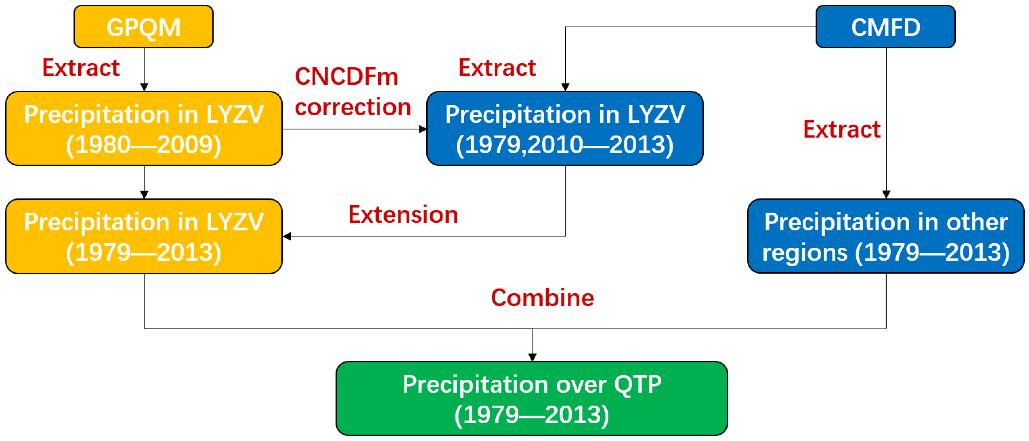
CMFD provides a high-resolution meteorological forcing dataset across China and has been evaluated for its temperature performance in western China. It shows better performance in surface temperature results in the QTP’s ungauged regions compared to other reanalysis data [11]; hence, the present study uses CMFD as the historical temperature source directly. However, CMFD precipitation is unverified in the western part of the QTP because of the lack of surface observational data, and it shows obvious bias in specified areas. What stands out is that it underestimates the precipitation in the LYZV compared with observations from ground stations in the Motuo and its immediate surrounding areas [48]. Hence, we adopt GPQM as a historical precipitation source in LYZV, which is validated with no obvious bias. GPQM considers observation stations both inside and surrounding the QTP [12]. It includes decades of gauge data from the south of the Himalayas, which can comprehensively reflect the precipitation characteristics of the QTP. To align the GPQM with the historical period of the HRP-QTP, we extend it using CMFD, and the extended method is shown in Figure 2.
Figure 2 employs three background colors to denote grid data from distinct sources: orange for GPQM data, purple for CMFD data, and green for the final 0.1° × 0.1° grid output of QTP’s precipitation data. Initially, we extracted QTP’s precipitation data, excluding the LYZV areas, from CMFD to serve as the historical precipitation source for other regions. Then, precipitation data for the LYZV were extracted from GPQM to the same grids as CMFD. Given that GPQM and CMFD share the same resolution, we applied GPQM data grid by grid to correct CMFD within the LYZV region. This correction allowed us to extend the GPQM data, ensuring that precipitation data from both sources matched the time dimension. We utilized an updated nonstationary CDF-matching method (CNCDFm), detailed in Section 2.5, for this correction. Finally, the extended GPQM precipitation data for LYZV were combined with the CMFD-extracted precipitation data for other regions, creating a comprehensive historical precipitation dataset for the entire QTP. This combined dataset will serve as the observed precipitation in subsequent steps.

2.4. Simulation and Prediction Data from GCMs

Seven CMIP6 GCMs were used to produce HRP-QTP (See Table 4). The GCM outputs were obtained from “https://esgf-node.llnl.gov/search/cmip6/ (24 March 2021)”. These GCMs were selected because precipitation, maximum temperature, and minimum temperature data were available for the 7 GCMs across most future scenarios. Moreover, they represent different resolutions, from 1.12° to 2.5°. In an assessment by Lun et al. [28], the 7 GCMs overestimate the precipitation of the QTP by 0.8–1.2 mm d−1 in the historical period, compared with CMFD. We interpolated them to a resolution of 0.1° and used historical data to correct their systemic bias. The CMIP6’s global simulation results of these climate models come from institutions worldwide, using different modeling methods. Compared with the representative concentration pathways (RCPs) of CMIP5, CMIP6 developed a new framework called shared socioeconomic pathways (SSPs) to quantitatively describe the relationship between climate change and socioeconomic development [26]. In this study, we selected SSP1-2.6, SSP2-4.5, SSP3-7.0, and SSP5-8.5 to represent different development and concentration pathways. These scenarios correspond to a sustainable development scenario, a medium challenge scenario for mitigation and adaptation, a high challenge scenario for mitigation and adaptation, and a high radiative forcing scenario with fossil fuels in the future period [49]. The four SSPs present varied global scenarios of radiative forcing, ranging from low to high. SSP1-2.6, SSP2-4.5, and SSP5-8.5 each align with the radiative forcing assumptions of RCP2.6, RCP4.5, and RCP8.5, respectively. In contrast, SSP3-7.0 serves as an alternative to the high radiative forcing scenario. Although it projects lower greenhouse gas concentrations than SSP5-8.5, it suggests that human society will face a greater risk of climate hazards [50]. We chose the first 3 SSPs to align our results with those of CMIP5 and SSP3-7.0 to represent a more likely high radiative forcing scenario.

2.5. Methods of Processing CMIP6 Data

Methods used to process CMIP6 data are divided into three steps: downscaling, multi-model ensemble forecasting, and bias correction. At first, we used a statistical method to downscale 7 GCM outputs from different resolutions. Secondly, a prior-based method was used to generate an ensemble forecast from GCMs. Finally, all results from the downscaling and multi-model ensemble were corrected by a nonstationary method. Details of the three steps are as follows:
(1)
Downscaling.
Most previous studies used linear interpolation methods to downscale GCM data and ignored the relationship between altitude and meteorological elements [2,4,25]. However, orographic studies demonstrated an approximately linear correlation between precipitation and temperature with elevation in high-altitude regions [51]. Several studies showed that it is necessary to consider altitude when generating high-resolution meteorological forcing [52,53]. Hence, we utilized ANUSPLIN (V4.36) to downscale the GCM data. ANUSPLIN is a software package that is based on the theory of thin-plate smoothing splines, and is an extension of linear regression, which considers distance, altitude, and other variables. Ma et al. [12] confirmed that ANUSPLIN is more accurate than inverse distance weighted and ordinary kriging methods in monthly precipitation interpolation over the QTP. In this study, ANUSPLIN was used to downscale daily precipitation and surface temperature, and altitude was considered a covariate in ANUSPLIN. More details about ANUSPLIN can be seen in the paper from M.F. Hutchinson and P.E. Gessler [54].
(2)
Multi-model ensemble forecast.
Due to the uncertainty in GCMs, the results of different climate models are widely distributed, and it is necessary to provide certain projection results for specific studies [55]. In this research, Bayesian model averaging (BMA) was used to produce a multi-model ensemble forecast result based on 7 GCM outputs in the historical period and 4 SSPs. BMA is a statistical method that is based on the posterior probability density functions (pdfs) of model predictions [56]. BMA, which is different from the multi-model average (MMA), could be described as a weighted average, as follows:
M B M A = k = 1 K w k M k
where MBMA is the output result of BMA, Mk is the output of model k, and w k is the weight of model k, denoting the posterior probabilities of model k conditioned. If we assume that the actual climate change process, y, is a combination of k model outputs, w k could be estimated based on fitting the data to the following relationship:
p y | M 1 , M 2 , M K = k = 1 K w k p y | M k
where the left side of Equation (2) denotes the pdf of the truth value in the historical period, and p y | M k denotes the conditional probability distribution of M k ; it represents the probability that y follows the pdf of the output from model k. When p y | M k is assumed to follow a normal distribution, it could be estimated as follows:
p y | M k = 1 2 π σ 2 e x p y t M k t 2 2 σ 2
with y t and M k t representing the y and M k values at time, t, respectively, and σ 2 is the variance of y M k . In this study, a Markov Chain Monte Carlo (MCMC) method proposed by Jasper et al. [57] was used to sample the weights of 7 GCM outputs. The weights were calculated based on historical GCM outputs in every 0.1° grid to maintain the spatial distribution characteristics of meteorological variables. The grid’s daily temperature and precipitation data obtained in Section 2.3 were used as truth values. BMA, which differs from taking the mean value of several models, considers the model’s performance during the training period, which could reduce the uncertainty of the ensemble result effectively [56,57,58]. MMA was also calculated in this study to compare with BMA.
(3)
Bias correction of nonstationary sequence.
Because climate processes are complex and cannot be described accurately by existing methods, all GCMs still have considerable biases in their output results. Previous studies have adopted many statistical methods to eliminate the systematic errors of the model, such as linear and nonlinear corrections or cumulative distribution functions (CDFs) [31,59,60]. Moreover, it is important to retain nonstationary information in future scenarios and avoid the occurrence of abnormality during bias correction. In this research, we adopted a nonstationary bias correction technique proposed by Miao et al. [61], called updated nonstationary CDF-matching (CNCDFm), to correct downscaled GCM data and BMA results. CNCDFm model methods can be presented as follows:
x ~ m _ p = I x , I x > 0 g x , I x < 0 0 , x m _ p = 0
I x = x m _ p + F o 1 F m _ p x m _ p F m _ h 1 F m _ p x m _ p
g x = x m _ p × F o 1 F m _ p x m _ p F m _ h 1 F m _ p x m _ p
where x denotes the meteorological variable from historical observations (o, denoted here as the reanalysis data obtained from Section 2.3) or models (m) during the historical period (h), current climate (c), or future projection (p) periods, F(·) is the CDF for a variable, and F−1(·) is its inverse. CNCDFm is an updated version of the CDF technique. By combining the method by Li et al. [62] with the method from Wang and Chen [63], it effectively retained nonstationary information in future scenarios and avoided the occurrence of abnormality. For instance, this approach could avoid negative values for precipitation or unreasonably high values (when the denominator on the right-hand side of Equation (6) is very small). Miao et al. [61] provided validation within the CMIP5 to approve the method’s efficiency.
Estimating the probability distribution of CDF is the key point of CNCDFm. We used the empirical cumulative distribution function (ECDF) to estimate the CDF in all periods for robust application. We used the 1979–2013 period as a training period to estimate Fo(·) and Fm-p(·) by the ECDFs of observed data and downscaled model output (obtained from Section 2.5 “Downscaling”). The wet day threshold was set at 0.1 mm/day to correct for the drizzle effect in precipitation data [31,64]. Model simulations in the historical period and the output of BMA were corrected in this step.

2.6. Effectiveness Evaluation of Methods

(1)
Applicability test of downscaling method.
This study designed an experiment to compare the effectiveness of different interpolation methods. Using CMA historical observations, 8 stations (white dots in Figure 1) were used for validation due to their long and complete series of observations. Observation data from the remaining 139 stations (black dots in Figure 1) were interpolated to the validation stations using three downscaling methods, namely, ANUSPLIN, inverse distance weight (IDW) [65], and original Kriging (OK) [65]; the latter two methods do not take altitude into consideration, which is used to compare with ANUSPLIN.
Here, IDW is used to represent linear two-dimensional interpolation, defined as follows:
Z x 0 = i = 1 n Z i d i i = 1 n 1 d i
where Z x 0 represents the interpolation result at verification station x 0 , Z i represents the observation from interpolation station i; n is equal to 139, and d i is the planar Euclidean distance in kilometers between x 0 and station i.
OK is used to represent non-linear two-dimensional interpolation, which is equivalent to thin plate spline interpolation without considering covariates. In this paper, OK is also based on ANUSPLIN; for technical details, please refer to Hutchinson and Gessler [54].
The interpolation results were compared with ground observation data by the Wasserstein distance (WD) [66] and quantile-quantile (Q-Q) plot. WD, also named the earth mover’s distance (EMD), is able to measure the distribution similarity between two samples very efficiently [67]; it could be defined as follows:
W D P 1 , P 2 = inf γ ~ P 1 , P 2 E x , y ~ γ x y
where γ ~ ( P 1 , P 2 ) denotes all possible joint probability distributions between P 1 and P 2 , i n f indicates the greatest lower bound, and E x , y ~ γ x y denotes the expectation of distance between samples x and y (which follow P1 and P2 distributions, respectively, representing the interpolated result and the observation at a verification station) when their joint distribution follows γ. In other words, WD indicates the minimum distance needed to move x into the same distribution as y . The smaller the WD, the closer the probability distribution between the interpolation results and the observations. The interpolation method with the minimum WD means that it most effectively captures the statistical distribution characteristics of the verification station.
Due to the inherently high randomness and uncertainty of weather systems, traditional Euclidean metrics, such as the mean absolute error (MAE) and root mean square error (RMSE), are limited to evaluating the effectiveness of interpolation methods [12]. This is because almost all interpolation methods struggle to capture the daily variations at unknown points [68]. In contrast, evaluating the fitting distribution characteristics through WD is more meaningful [69]. Long-term climate change studies may not necessarily require precise daily precipitation or temperature data for specific days, but accurate probability distribution characteristics within specific time periods are essential. This is crucial for research on extreme statistics and is important for both historical simulations and future predictions. Therefore, we adopt the WD as the evaluation metric.
(2)
Statistical validation of bias correction.
To evaluate the absolute mean bias (AMB) of each model before and after correction, we verified the validity of the correction method. The evaluation was performed as follows: First, we randomly selected 20 years from the historical period of 34 years; GCM outputs from this 20-year period were divided into two equal-length parts, x m _ h and x m _ p , as seen in Equations (5) and (6). Secondly, x m _ p was corrected by x m _ h and reanalysis data in the corresponding period; the pre-correction and post-correction AMBs against these observations are calculated as follows:
A M B = x o x m p n
where xo denotes the values extracted from the reanalysis data obtained in Section 2.3, and n denotes the sample size in the validation period.
The above steps were repeated 10 times in each 0.1° resolution grid to ensure the performance of the multi-model ensemble forecast. Bias correction was evaluated by the mean value of the results from these 10 iterations to guarantee the robustness of the evaluation [50], and the AMB was taken using absolute values to prevent the positive and negative from canceling out.
Quantile bias (QB) is used as a supplementary test to evaluate the ability of bias correction to extreme values. The QB of the specified percentage p can be defined as follows:
Q B = F m h 1 p F o 1 p
where F m h 1 and F o 1 are the same as in Equations (5) and (6), and F m h 1 is estimated by ECDF before and after correction.
(3)
Evaluation of multi-model uncertainty.
Uncertainty is a key factor affecting the usability of model prediction results; the signal-to-noise ratio (SNR) was used to quantify the proportion of valid information amid uncertainty. SNR is defined as follows:
S N R = D S D N
with
D S = x ¯ x h
D N = 1 n + 1 i = 1 n x i x ¯ 2
where, x ¯ means the prediction result of MMA, x h denotes the historical simulation result, n denotes the number of climate models, and x i denotes the prediction result of model i. It indicates that reliability is higher than uncertainty when SNR is greater than 1. Furthermore, because SNR is dimensionless, it can be used to compare different variables.

3. Results

3.1. Performance of Downscaling Methods in the Historical Period

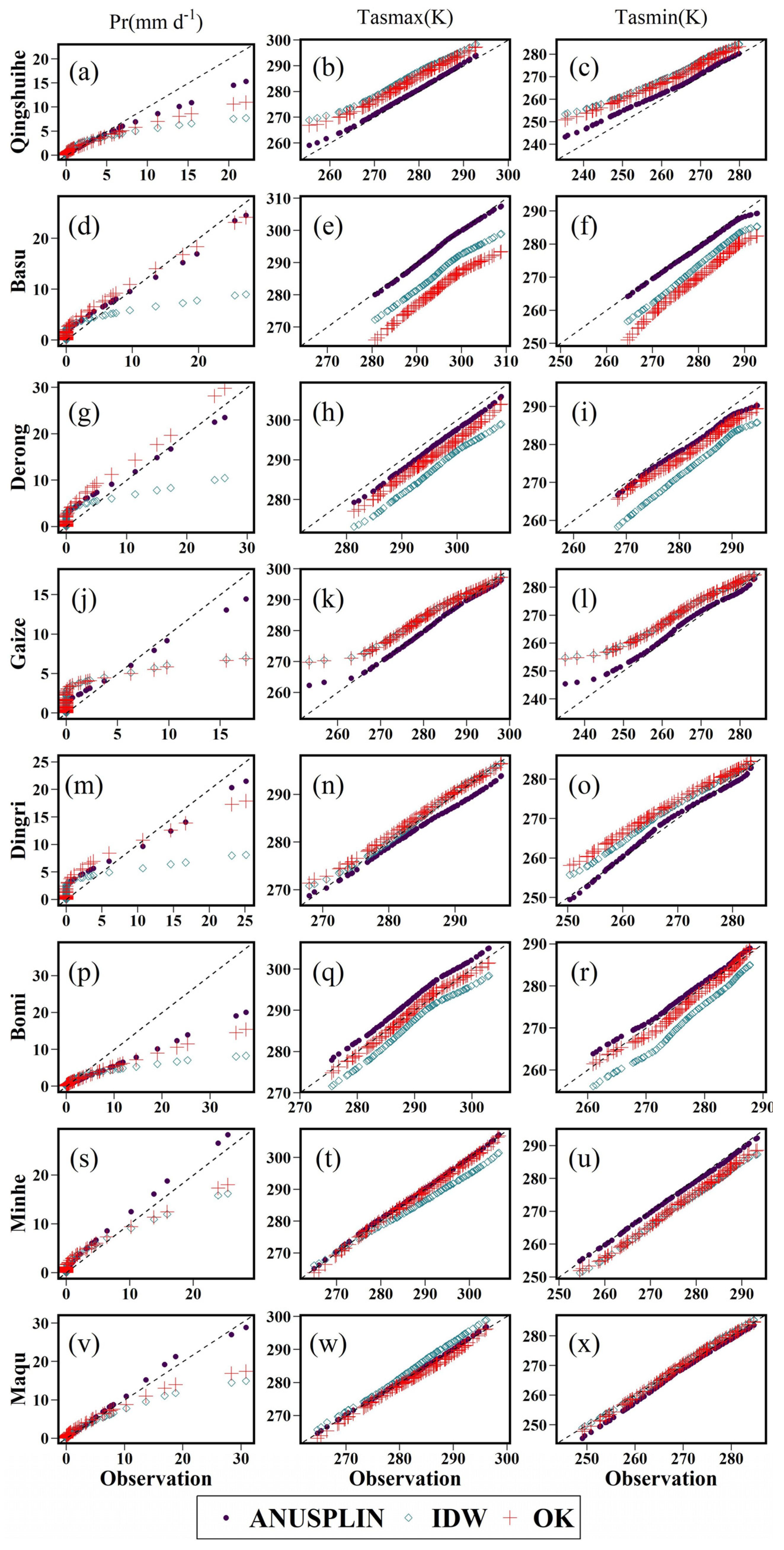
Table 5 and Figure 3 display the effects of different interpolation methods. ANUSPLIN shows the best-fitting results at all eight validation stations for precipitation as well as the minimum temperatures. For maximum temperature, it also presents the best-fitting results at six validation stations. This suggests that considering altitude as a covariate can significantly reduce statistical distribution errors in downscaling. According to Table 5, ANUSPLIN achieves the smallest average WDs (0.49 mm d−1 for precipitation, 1.18 K for maximum temperature, and 1.39 K for minimum temperature, respectively) among the three downscaling methods for all variables. Only in the cases of maximum temperature at Dingri and Bomi and minimum temperature at Bomi and Maqu do IDW and OK methods perform slightly better than ANUSPLIN, respectively.
Figure 3 demonstrates that ANUSPLIN provides a better fit to the ‘x = y’ line at most stations. For precipitation, OK consistently overestimates light rain and underestimates heavy rainfall, as indicated by the red crosses in Figure 3. IDW exhibits the same issue at Gaize and Qingshuihe stations, represented by blue prisms in Figure 3a,j. At other stations, IDW tends to overall overestimate precipitation. For temperature, both IDW and OK consistently overestimate temperatures at high-altitude stations (Qingshuihe, Gaize, and Dingri, whose altitudes are higher than 4000 m) and underestimate at relatively low-altitude stations (Basu, Derong, and Bomi, whose altitudes are lower than 3000 m). This is likely because they do not account for the linear relationship between temperature and elevation. Overall, ANUSPLIN (indicated by purple dots in Figure 3) outperforms the other two methods in addressing the above issues, especially when fitting precipitation extremes, which is crucial for regional hydrological research.
Overall, the results in this section suggest that ANUSPLIN is available for the meteorological element interpolation of the QTP; that is, it is more reasonable than IDW and OK in the performance of precipitation extremes and temperatures. This advantage is likely attributed to its superior ability to model the nearly linear relationship between climate variables and altitude, taking elevation into account as a significant covariate. It also highlights that neglecting altitude’s impact in downscaling efforts within the QTP can lead to significant statistical distribution biases, a finding that aligns with prior studies [8,12,70,71,72].

3.2. Multi-Model Ensemble and Bias Correction Performance

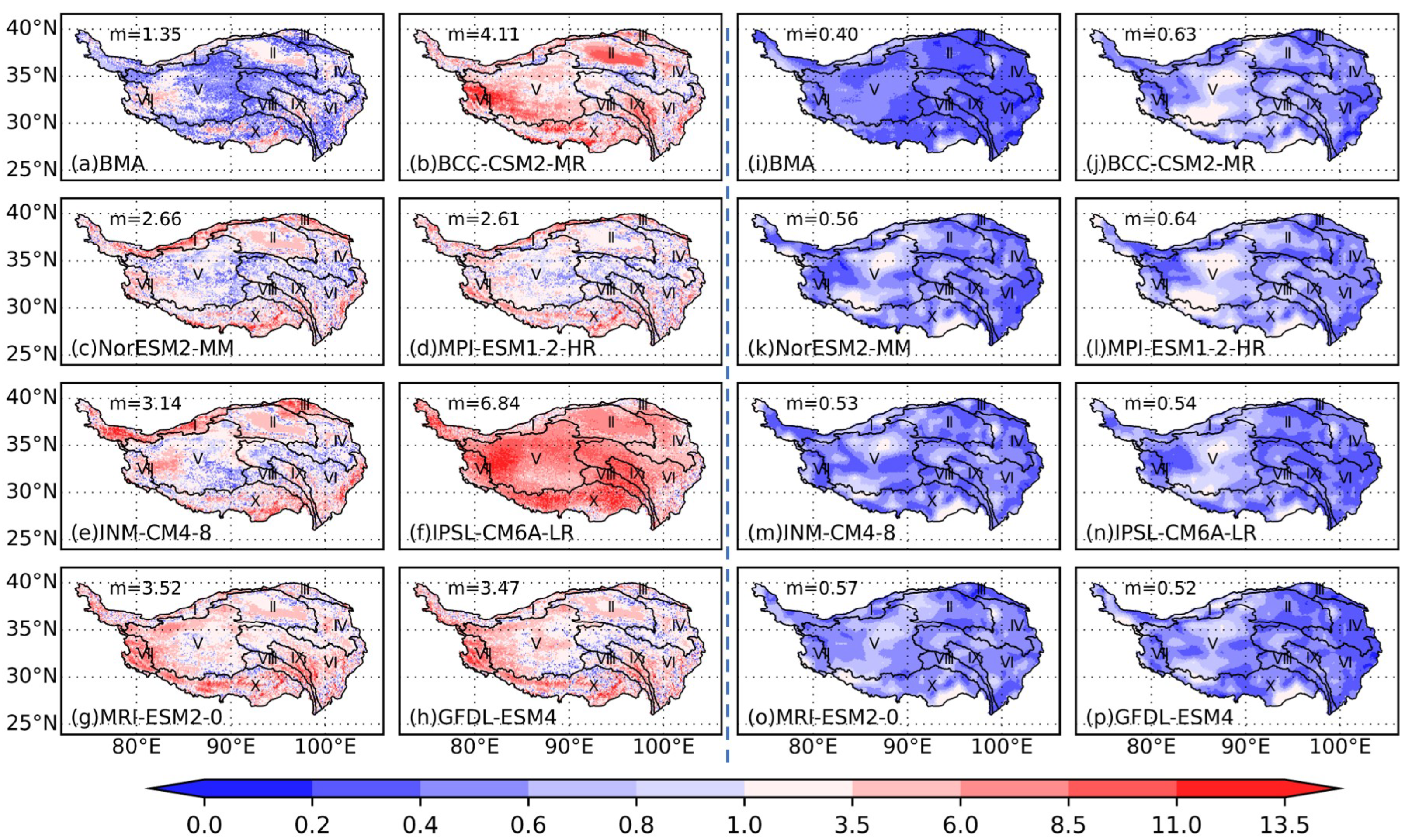
The AMBs before and after correction are shown in Figure 4, Figure 5 and Figure 6, showing a substantial reduction in the AMBs after bias correction across all three variables from the seven GCMs and BMAs for the historical period (1979–2013). The outputs of these three variables from the seven GCMs all showed large biases before correction, as depicted in Figure 4, Figure 5 and Figure 6b–h. For precipitation, the AMBs of seven GCMs ranged from 0.87 to 1.73 mm d−1, some of them were even higher than the mean precipitation over the QTPs (1.24 mm d−1 approximately); the high bias value (≥3.00 mm d−1) occurred in the southeast of the QTP, covering the southern parts of IDR, YLZBR, YZR, MKR, and SWR, before bias correction (Figure 4b–h). For temperature, seven GCM AMBs ranged from 1.35 to 6.84 K (maximum surface temperature, Figure 5b–h) and from 1.23 to 10.63 K (minimum surface temperature, Figure 6b–h). For maximum surface temperature, the high bias value (≥8.50 K) occurred at the edge of QDB and most of TMR, IDR, and YLZBR; for minimum surface temperature, the high bias value (≥8.50 K) occurred in the western part of the QTP (TMR, IDR, and western parts of IQTB and YLZBR) and small parts of QDB, before bias correction. Therefore, such uncorrected data cannot be used for climate research and decision-making at the regional scale [31]. After bias correction, the GCMs’ absolute mean bias was reduced to an acceptable range. For precipitation, it was from 0.13 to 0.19 mm d−1 (about an 85% to 89% reduction Figure 4j–p). For temperature, they were from 0.40 to 0.64 K (maximum surface temperature, Figure 5j–p) and from 0.37 to 0.55 K (minimum surface temperature, Figure 6j–p). High values only occurred in smaller areas compared with uncorrected data. For precipitation, only NorESM2-MM exhibited high AMB (≥3.50 mm d−1) in a small part of LYZV (Figure 4k). The reduction in bias for mean annual precipitation, as well as the maximum and minimum temperatures, demonstrates the effectiveness of our bias correction based on CNCDFm.
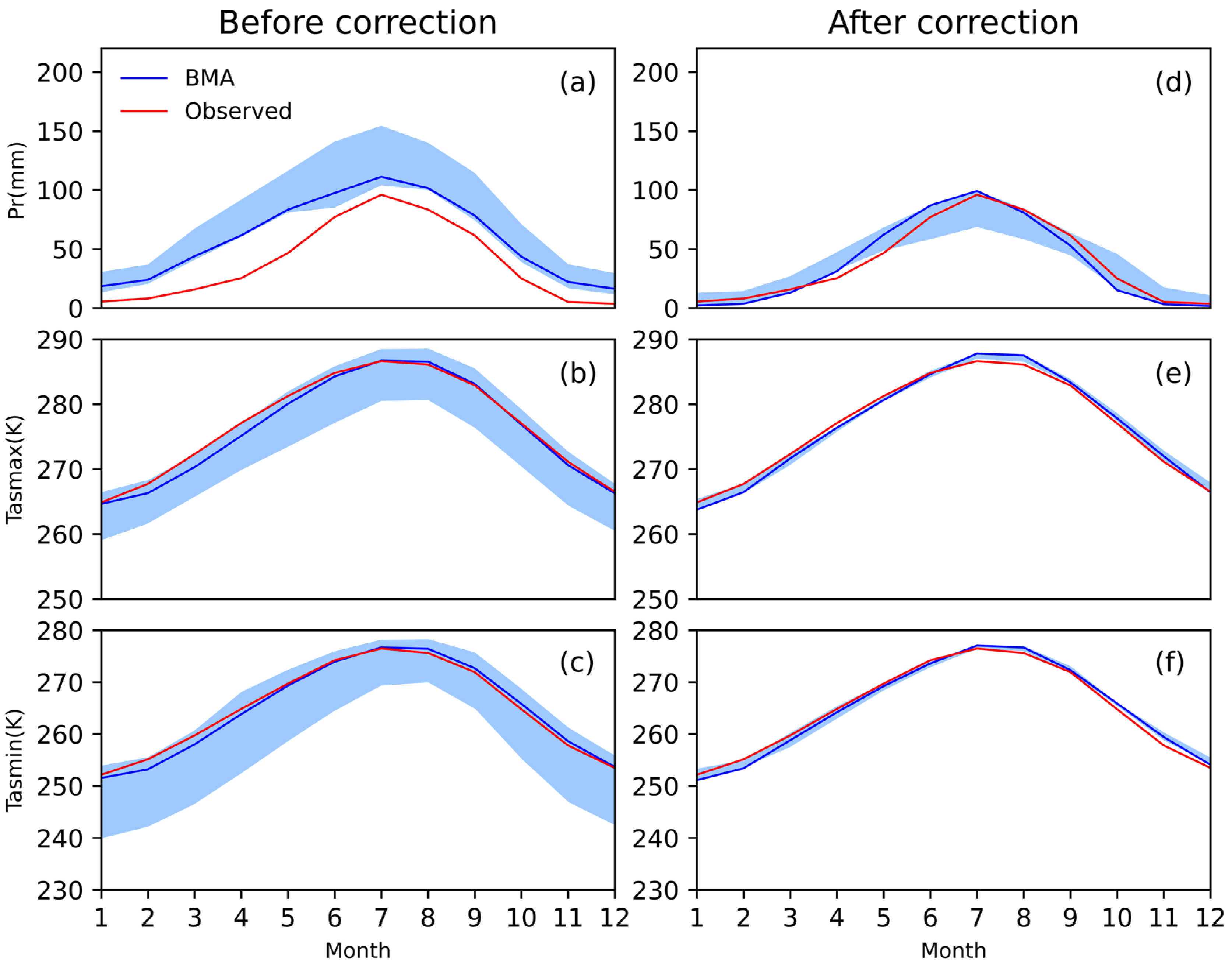
To verify the correctness of the corrected data, we separately analyzed the seasonal cycles before and after bias correction (Figure 7) and the mean annual values after bias correction (Figures S1–S3) for three variables over the historical period. The data show a wet bias for precipitation and a relatively cold bias for temperature in the GCMs’ seasonal cycles compared to observations from before bias correction (Figure 7a–c), typically due to systematic errors overlooking the monsoon effect and surface meteorological processes in GCMs [27,28,73]. Compared to the uncorrected data, the seasonal cycles of the corrected data more closely align with observations (Figure 7d–f), as CNCDFm has corrected biases for both high and low values [61]. The uncertainty in GCM outputs has been significantly reduced post-bias correction, as evidenced by the narrowed ranges (shaded areas in Figure 7d–f). Figures S1–S3 show the spatial distributions of mean annual values for the corrected data, indicating a strong agreement with observations. Precipitation data, in particular, show a consistent decline from the southeast to the northwest of the QTP (Figure S1c–i), aligning with prior studies [7,8,74]. Regarding temperature, all seven GCMs indicate lower values in the IQTB due to its high altitudes and latitudes, with higher temperatures primarily found in the southeastern part (Figures S2c–i and S3c–i), which is consistent with orographic findings [51]. Overall, our results indicate that the CNCDFm method has produced a reasonably corrected dataset based on CMIP6 GCMs, which is suitable for climate impact studies in the QTP.
At the same time, we calculate the mean biases, seasonal cycles, and mean annual values for the BMA (as shown in Figure 4, Figure 5 and Figure 6a,i, the blue line in Figure 7 and Figures S1–S3b). Before the bias correction, BMA exhibited the lowest absolute mean bias (AMB) compared to the outputs from the seven GCMs, attributed to the consideration of the models’ posterior probability distributions (Figure 4, Figure 5 and Figure 6a). After bias correction, BMA showed the lowest AMB for precipitation (Figure 4i) and avoided the high-temperature AMB that occurred in every individual model (Figure 5i and Figure 6i). In terms of seasonal cycles, the corrected BMA data align well overall with observations after bias correction (Figure 7d–f). Furthermore, the spatial distribution of the corrected BMA output is consistent with the observations (Figures S1–S3b). Overall, BMA provides a robust multi-model ensemble forecast result for precipitation, as well as maximum and minimum temperatures across the Tibetan Plateau.
Studying extreme events is a crucial aspect of climate change research. To evaluate the performance of bias correction in extremes, the QBs for uncorrected and corrected BMA 95th percentiles were compared against observations for the historical period (1979–2013) for three variables, as shown in Table 1 (Figure S4). The analysis revealed that biases in the 95th percentiles were successfully mitigated, with the corrected BMA data bias approaching 0 (Figure S4b,c,f) compared with the uncorrected. Thus, the corrected data also demonstrate improved performance for extreme values.

3.3. Future Climate Change Projection in the QTP

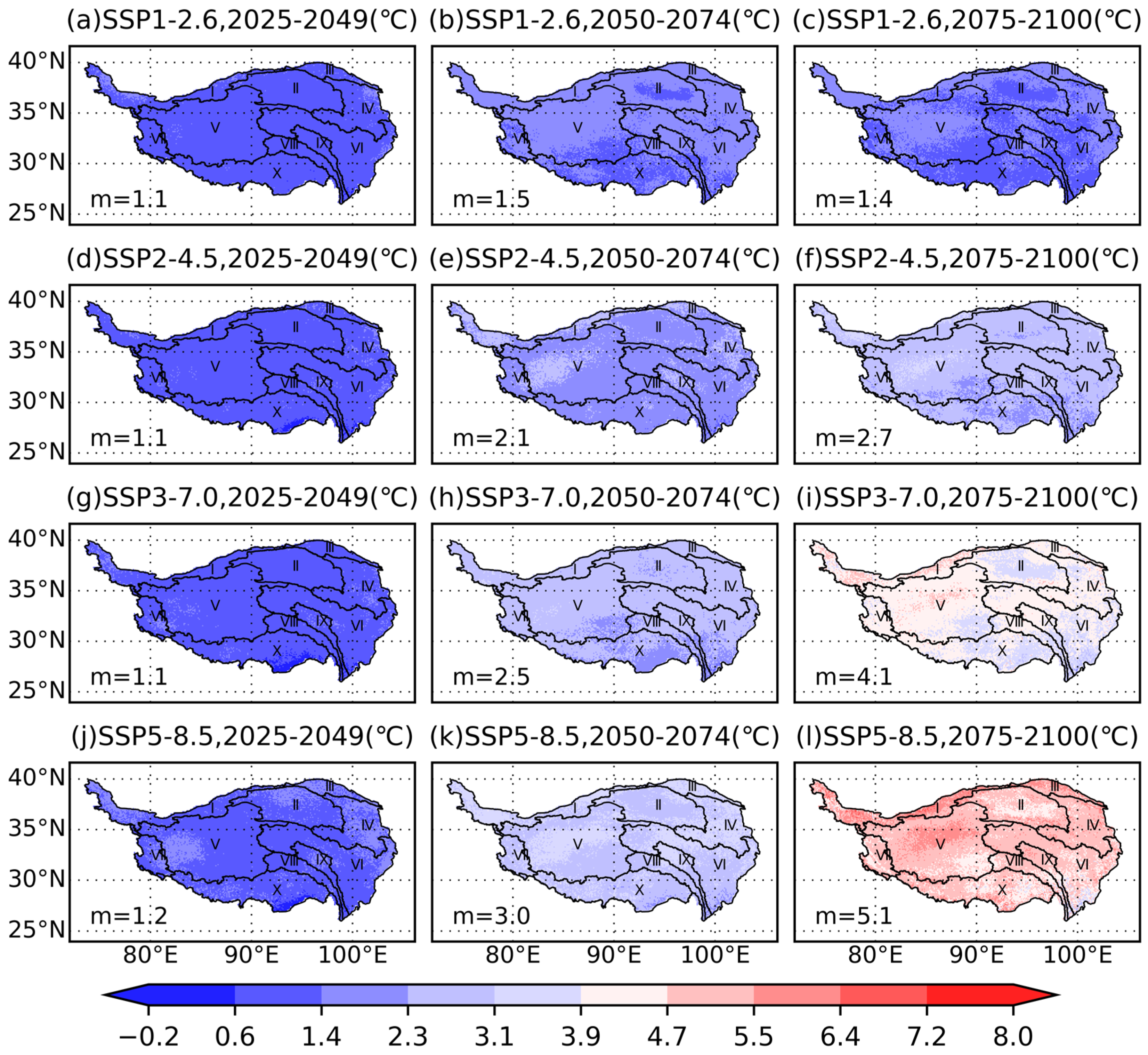
Projected changes in precipitation and maximum/minimum surface temperatures in the QTP for the 21st century, based on outputs from the corrected BMA and seven GCMs, span from 2025 to 2100. We estimated these changes for the near (2025–2049), medium (2050–2074), and far (2075–2100) future periods, using a historical baseline of 1985–2013, across all four scenarios (SSP1-2.6, SSP2-4.5, SSP3-7.0, and SSP5-8.5), as shown in Figure 8, Figure 9 and Figure 10. Overall, the projections indicate consistent warming and wetting trends for the QTP in the 21st century, aligning with historical trends [6,75], except for SSP1-2.6, where the rate of increase in precipitation and temperature is projected to slow down significantly in the far future (Figure 8, Figure 9 and Figure 10c). Compared to the low radiative forcing pathway (SSP1-2.6), high radiative forcing pathways (SSP3-7.0 and SSP5-8.5) have considerably large increases in precipitation and temperature. For instance, under SSP5-8.5, mean precipitation is projected to rise by 26.8% in the far future (Figure 9i), with mean maximum and minimum surface temperature increases of 5.1 °C and 5.7 °C, respectively (Figure 9 and Figure 10i). Excessive warming may accelerate the retreat of plateau glaciers, especially in the TMR and IQTB regions. Furthermore, it shows a consistent spatial pattern in the different SSPs. For instance, a higher precipitation increase was found in the northern parts of the IQTB and IDR, TMR, and QDB under SSP3-7.0 and SSP5-8.5 in the far future.
Future precipitation and temperature were also estimated in 10 subregions based on corrected BMA (Tables S1–S3), as seen in the Supplementary Materials, Figure 8, Figure 9 and Figure 10. The projections indicate increases in the mean annual precipitation and maximum and minimum temperatures across these subregions under middle and high radiative forcing pathways (SSP2-4.5, SSP3-7.0, and SSP5-8.5), with significantly higher increases across high radiative forcing scenarios compared to low radiative forcing ones, aligning with projections for South Asia [31]. Notably, under SSP3-7.0 and SSP5-8.5, all three variables are projected to continue to rise, which is consistent with the overall trend across the QTP. Under SSP1-2.6, the precipitation trend in HXB, IDR, IQTB, QDB, and TMR in the far future is lower than in the middle future, a trend likely attributed to the mitigating effects of reduced greenhouse gas concentrations on climate change. Overall, the bias-corrected dataset produced a reasonable projection for subregions in the QTP, and it is available for hydroclimatic research at the regional scale.
Figure 11 illustrates the time series for BMA (represented by solid lines) and MMA (represented by dotted lines), demonstrating a more continuous growth trend in temperature (both maximum and minimum) in SSP2-4.5, SSP3-7.0, and SSP5-8.5, as observed after applying a 30-year moving average. Conversely, a distinct turning point occurs mid-century in SSP1-2.6, where warming shifts to cooling across all subregions, highlighting the impact of carbon emission limitations on regional temperature trends. This warming trajectory parallels the global warming process projected by the IPCC’s Sixth Assessment Report (AR6), which predicts a global surface temperature increase of 4 °C by the century’s end under SSP5-8.5 compared to 1995–2014 [76]. Notably, the rate of warming in the QTP exceeds the global average, underscoring the region’s sensitivity to climate change, as historically observed [6].
Furthermore, noteworthy changes in the spatial distribution of precipitation and temperature across the Tibetan Plateau merit attention. Specifically, future projections indicate a significant increase in precipitation rates in IDR, QDB, TMR, and the northwest of IQTB (Figure 8 and Figure 11(b1,c1,e1,g1), Table S1), which is not only far ahead of global future growth but also far ahead of the rest of the QTP. The future moistening trend in the northern region is consistent with historical trends. Zhang et al. estimated a historical precipitation growth rate of 1.5–3.0 mm yr−1 in this area [77]. The significant growth rate may be partly due to the historically low precipitation in this area (Table S1), and partly due to the enhanced atmospheric circulation caused by warming [78], which accelerates the local moisture recycling and increases the input of external moisture [77,79,80]. However, the drastic change in precipitation is bound to have a profound impact on the regional hydrological cycle. For temperature, there is no obvious spatial differentiation in the near future change (Figure 9 and Figure 10a,d,g,j), while in the far future, spatial differentiation is prominent. For instance, IQTB and TMR have shown higher warming than other regions in SSP5-8.5, which may be due to the underlying positive feedback of the radiation absorption and will accelerate the ablation of regional glacial permafrost [81,82,83,84]. These spatial differences highlight the necessity of high-resolution projection for research in the QTP.
Table S4 provides statistics on the mean rate and change rate of the annual maximum five-day precipitation for future years based on BMA. Notably, IDR exhibits the highest change rate among the 10 sub-regions in the vast majority of scenarios and periods, with growth rates reaching 22.9 to 41.2% in the distant future. The significant increase in the annual maximum five-day precipitation, as an indicator of extreme precipitation, implies an elevated risk of hydrogeological disasters, such as floods, landslides, and debris flow [85,86,87]. Most areas in IDR are above 4000 m, given its higher elevation (Figure 1). Geological disasters in this region will likely cause more significant damage downstream [88], highlighting the need for enhanced observation and monitoring in this area.

4. Discussion

In the present study, the effectiveness of downscaling and bias correction methods were evaluated. The projection results are presented at a basin scale and compared with previous research. Such results could verify the rationality of HRP-QTP, but some issues remain that deserve further discussion.

4.1. Availability of Reanalysis Precipitation

In numerous areas worldwide, the scarcity of observation data significantly hampers the execution of various environmental research initiatives, especially for precipitation [89]. He et al. [11] evaluated the accuracy of CMFD in simulating conditions in regions across western China that are poorly monitored, using additional data from measuring stations in IDR, IQTB, YZR, and SWR. The findings indicate that CMFD provides a more accurate representation of temperature in areas of the QTP that lack direct observational data, leading us to adopt CMFD temperature data as a proxy for historical observations. However, the dataset’s precipitation measurements have not been similarly validated in the QTP.
Through the extension and correction of GPQM and CMFD data, we derived a combined dataset aimed at correcting the CMFD’s underestimation of precipitation in the LYZV area, using additional station information from GPQM beyond the QTP. The historical annual mean precipitation across 12 subregions of the QTP (as shown in Figure 12) was estimated based on the data generated in Section 2.3. The results indicate that the QTP’s historical annual mean precipitation is 456 mm/year, with a slight increase over historical periods, aligning closely with ground station measurements [75]. Spatial analysis reveals that the eastern and southern subregions, such as MKR, SWR, YZR, and YR, exhibit higher precipitation levels (602 mm/year, 653 mm/year, 598 mm/year, and 500 mm/year, respectively) compared to the central and northern subregions (HXB, IQTB, QTB, and TMR, with annual mean precipitation of 241 mm/year, 261 mm/year, 168 mm/year, and 145 mm/year, respectively), reflecting the patterns of water vapor transport in the QTP [8,47]. Notably, due to its high precipitation, at approximately 3120 mm/year, the YLZBR region records the highest precipitation among all subregions at 1108 mm/year.
Generally, gauge data are considered the most accurate precipitation data [90]. However, it is difficult to estimate and validate LYZV precipitation due to a lack of observations (Figure 1), and reanalysis based on multi-source data is the only method currently available to estimate precipitation in LYZV. Due to differences in methods and data sources, different reanalysis datasets have demonstrated a wide range of estimated results, ranging from 1000 mm/year (for instance, He et al. [11] estimated the LYZV annual mean precipitation at 1001 mm/year by combining upstream ground station data with satellite reanalysis data) to 4000 mm/year (the estimation by Ma et al. [12] is 3011 mm/year using interpolation of downstream gauge data; the estimation by Li et al. [8] is from 1000 to 4000 mm/year at different altitudes using grid data from the Global Precipitation Measurement, GPM). We tend to use the higher precipitation estimates for LYZV because they are more consistent with precipitation characteristics in the southern Himalayas, which are close to the same altitude regions in Bhutan [45] and corroborate early findings by Yang et al. [91]. Nonetheless, given the QTP’s extensive area and complex topography, different reanalysis datasets offer distinct advantages across various regions [20]. Accurately estimating precipitation across the QTP remains an unresolved challenge that requires further observational evidence.

4.2. Availability of Downscaling Methods

In Section 3.1, we present a simple comparative experiment to demonstrate the effectiveness of ANUSPLIN, which takes elevation into account, in downscaling climatic elements in the QTP. Herein, IDW represents linear two-dimensional interpolation, and OK represents non-linear two-dimensional interpolation, both of which are compared with the non-linear three-dimensional interpolation of ANUSPLIN.
The interpolation result of IDW equals the weighted average of all known stations, with the weights being inversely proportional to the distance between the known points and the interpolation point. Therefore, once the locations of the sites are determined, the interpolation relationship is also established. OK and ANUSPLIN perform interpolation by constructing non-linear relationships to fit the climate surface of known stations [54]. The fitting relationship is time-varying (in this study, both use annual fitting). The difference lies in that ANUSPLIN considers covariates.
Compared to ANUSPLIN, the limitation of two-dimensional interpolations lies in their focus on spatial relationships between stations, leading to a reliance on information from nearby stations and overlooking the decisive role of elevation on plateau climates. Taking temperature as an example, a common rule is that temperature decreases with the increase in elevation [7]. The elevation of stations near the Basu station is higher than that of Basu (Figure 1), with the nearest five having an average elevation of 3082 m, significantly higher than Basu’s 2589.2 m. This results in the two-dimensional interpolations significantly underestimating the temperature at Basu (Figure 3e,f). This bias is corrected in ANUSPLIN. Furthermore, the fitting performed by ANUSPLIN is time-varying, meaning that if the correlation between climate elements and elevation changes in future scenarios, the new correlation can also be captured [92]. This reduces the systematic bias caused by limitations in fitting capability during downscaling.
However, downscaling climate models continues to be an exceedingly complex issue. Identifying the optimal downscaling method and understanding how systematic errors are transmitted during the downscaling process urgently require further investigation. This study merely demonstrates the viability of applying ANUSPLIN in plateau areas.

4.3. Uncertainty and Reliability in Future Projections

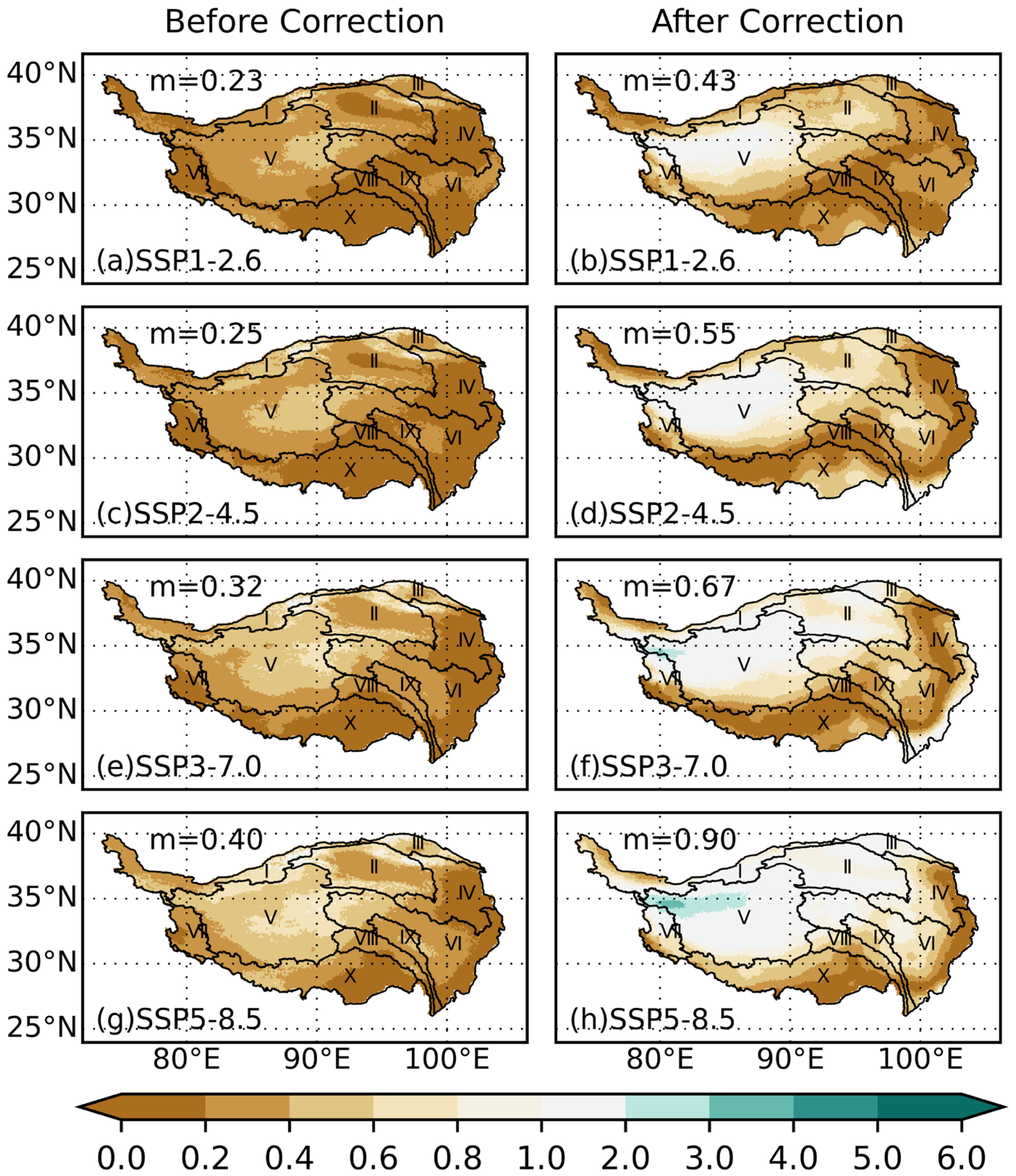
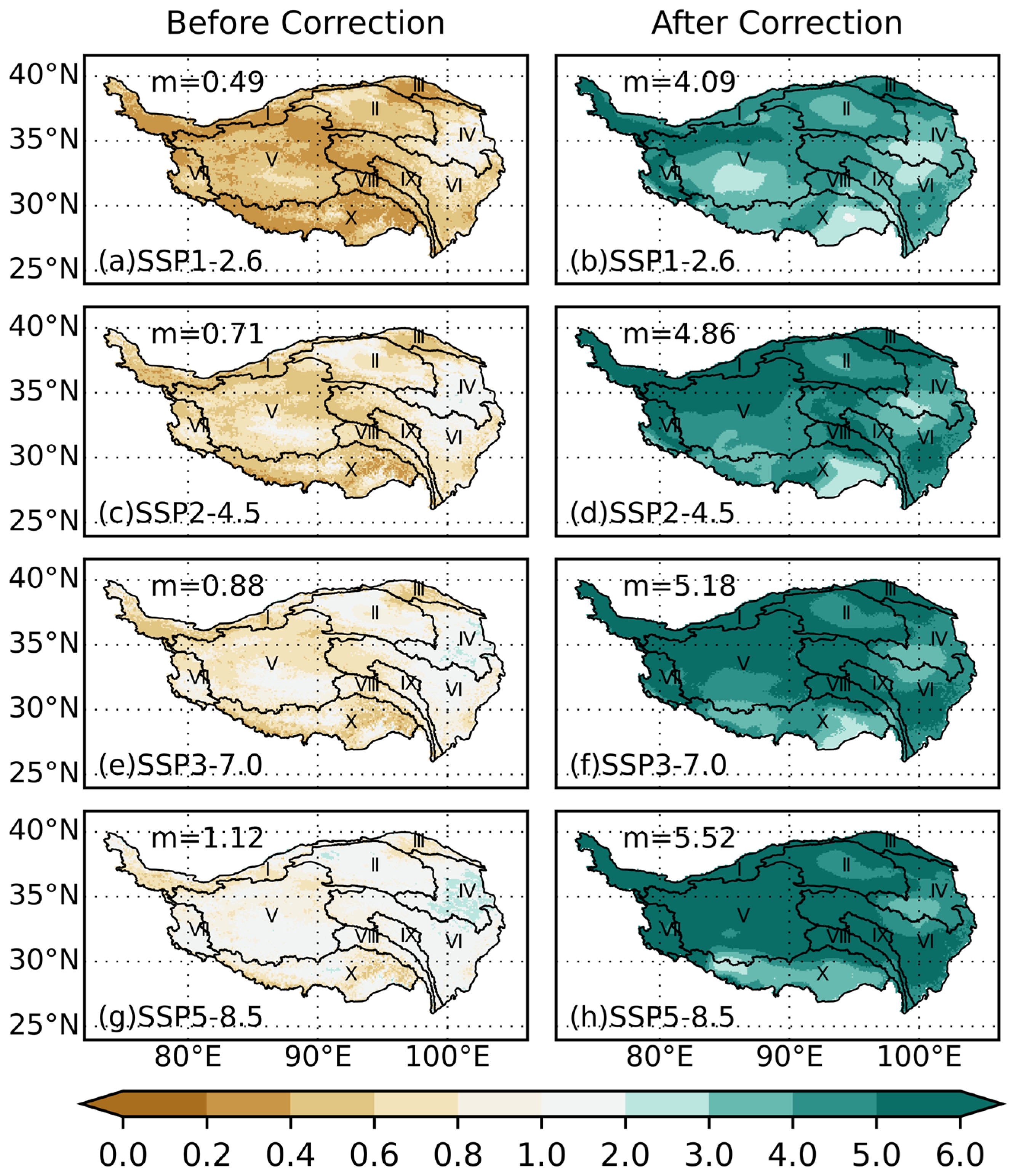
Previous studies have indicated significant divergence in climate projections for the QTP from GCMs [27,28,30], leading to low SNRs. As shown in Figure 13, Figure 14 and Figure 15, bias correction significantly increases the SNR for three variables: for precipitation, the SNR range increased from 0.23–0.40 to 0.43–0.90; for temperature, it rose from 0.37–1.12 to 3.67–5.52. This suggests that bias correction effectively eliminates systemic model biases, making future model projections more reliable. However, reliability varies greatly among different variables. For temperature, both maximum and minimum, the SNR exceeds 1 in all subregions (Figure 14 and Figure 15) after correction, indicating a clear trend in the future temperature rise and reduced uncertainty. In contrast, precipitation shows an overall SNR below 1, with several regions, including LYZV, MKR, SWR, YZR, and YR (Figure 14b,d,f,h), exhibiting SNRs far below 1. This suggests that future changes in precipitation for these regions are not pronounced and are subject to considerable uncertainty, a conclusion supported by Figure 11(d1,f1,h1,i1,j1).
We compare our findings with those from Cui et al. [30], who projected precipitation for several major river basins using a broader set of GCMs, albeit at a lower spatial resolution. Their results, showing SNRs in Table 6, reveal that SNRs exceeding 1 only occur in the Indus, Mekong, Salween, and Yellow River basins under SSP2-4.5 when future temperatures increase by 3 °C. Contrasting these findings with ours (Figure 13, Figure 14 and Figure 15) indicates that the SNRs for multi-model projections remain consistently low, suggesting that merely increasing the number of predictive models does not necessarily enhance prediction reliability. Mechanistically, precipitation predictions depend on factors such as wind, humidity, and aerosols [93,94,95]. The approximation and parameterization of these factors in GCMs might introduce more uncertainty into precipitation forecasts than temperature forecasts.
Furthermore, while current studies often prioritize MMA, we advocate for BMA based on our belief that historical simulations can inform and constrain future climate predictions. Unlike BMA, MMA does not incorporate prior information from historical periods, which is particularly relevant for temperature projections where the differences between BMA and MMA are minimal. However, for precipitation, especially in regions like IQTB, MKR, and YZR post-2050, BMA projections are significantly higher than those from MMA, as illustrated in Figure 11. Precipitation, subject to considerable model uncertainty, poses challenges. Ferguglia et al. [96] demonstrated that the emergent constraint approach—relying on a physically explainable link between historical and future data—does not robustly address systematic uncertainties, indicating the limitations of depending solely on multi-model precipitation outcomes. However, due to the lack of historical data and the unclear precipitation mechanism, statistical correction is still a widely used reanalysis method in existing research. We retained the correction results of each model in the final forecast dataset provided for further study.

5. Conclusions

The QTP serves as Asia’s most crucial water source, with climate change in the QTP poised to profoundly affect water security and geopolitical relations across the continent. The region’s complex terrain necessitates high-resolution climate projections to underpin studies on regional climate change and guide adaptation strategies. To address this need, our research developed a high-resolution projection by utilizing reanalyzed meteorological datasets alongside outputs from seven GCMs. We employed a downscaling method that accounts for altitude variations and implemented an updated nonstationary bias correction technique, both of which were rigorously tested for validity. Key findings from our study include the following:
  • There is an approximately linear relationship between climatic factors and altitude in high-altitude areas. Therefore, the ANUSPLIN software, which incorporates DEM as a covariate, can more accurately fit the probability distributions of meteorological elements. Ignoring altitude’s impact on the distribution of meteorological elements during downscaling leads to the overestimation or underestimation of temperatures and overlooks extreme precipitation events. Thus, incorporating elevation data as prior information in downscaling processes is crucial. Despite significant systematic biases in GCM simulations and predictions for the QTP climate, these can be substantially mitigated by employing an advanced nonstationary bias correction method, CNCDFm. For example, this method has been shown to minimize the deviation of extreme values to nearly zero. Consequently, our research enhances the applicability and accuracy of GCM results for regional studies in the QTP.
  • Based on high-resolution projections, the QTP is expected to continue experiencing warming and wetting trends. The projected temperature change range remains consistent across the QTP subregions, mirroring the historical trend where the QTP temperature increase surpasses the global surface temperature rise. Under the Shared Socioeconomic Pathway SSP1-2.6, the region is anticipated to reach a warming inflection point by the mid-21st century. Furthermore, future precipitation projections indicate significant spatial variations, with growth rates in regions such as IDR, IQTB, QDB, and TMR far exceeding the global average. Such marked increases in temperature and precipitation are likely to fundamentally transform the regional hydrological cycle.
  • Two significant challenges hinder the accurate forecasting of future precipitation trends in the QTP. Firstly, the historical period lacks global high-resolution precipitation data that are convincing enough for detailed analysis, especially in ungauged regions such as the IQTB, YLZBR, TMR, and IDR. This scarcity complicates the analysis of historical precipitation changes and the calibration of GCMs. Secondly, there remains substantial uncertainty in GCM projections. While bias correction techniques can mitigate some systematic biases inherent in GCMs, the reliance on historical data to constrain future precipitation projections proves to be less effective than for temperature, rendering precipitation forecasts less reliable. This uncertainty also leads to significant discrepancies between the precipitation forecasts of BMA and MMA, both of which indicate an increasing trend across all basins. Further research is imperative to enhance the reliability of multi-model precipitation predictions.
Despite the limitations outlined above, this research provides a high-resolution future prediction for regional-scale studies of the QTP that is openly accessible for further testing, research, and decision-making purposes.

Supplementary Materials

The following supporting information can be downloaded at https://www.mdpi.com/article/10.3390/atmos15040434/s1, Figure S1: Mean annual precipitation (mm) for (a) observation and corrected data of (b) BMA and (c–i) individual GCMs for the historical period (1979–2013). The mean value of annual precipitation across the entire QTP is denoted in each subgraph as m; Figure S2: The mean annual value is the same as in Figure S1 but for the maximum surface temperature; Figure S3: The mean annual value is the same as in Figure S1 but for the minimum surface temperature; Figure S4: Quantile Bias (QB) of BMA in the 95th percentile of precipitation, as well as maximum and minimum temperatures, for the historical period (1979–2013); Table S1: Subregion-wise BMA-projected change in the mean annual precipitation (mm), the division of three futures is the same as in Figure 12, and the historical mean is from 1985 to 2010; Table S2: Subregion-wise BMA-projected change in the maximum surface temperature (°C); Table S3: Subregion-wise BMA-projected change in the minimum surface temperature (°C); Table S4: Subregion-wise BMA-projected change in the average annual maximum five-day precipitation (mm).

Author Contributions

Conceptualization, X.S. and K.W.; methodology, X.S. and K.W.; validation, K.W., S.Y., F.L. and J.S.; formal analysis, K.W.; data curation, K.W. and Y.Z.; writing—original draft preparation, K.W.; writing—review and editing, K.W., X.S., F.L. and Y.Z.; visualization, K.W. and S.Y.; supervision, F.L.; project administration, F.L.; funding acquisition, F.L. and Y.Z. All authors have read and agreed to the published version of the manuscript.

Funding

This research was funded by the Second Tibetan Plateau Scientific Expedition and Research Program (STEP, no. 2019QZKK0207-02), the National Natural Science Foundation of China (no. 51909275), IWHR Research & Development Support Program (no. WR110145B0052021), and Qinghai Central Government Guided Local Science and Technology Development Fund Project (no. 2022ZY020).

Institutional Review Board Statement

Not applicable.

Informed Consent Statement

Not applicable.

Data Availability Statement

All bias-corrected GCMs and BMA output for different scenarios were stored in Network Common Data Form (NetCDF) files. These files were named following a standard form as MODEL_scenario_variable.nc. For instance, bias-corrected precipitation from GFDL-ESM4 in SSP1-2.6 was named GFDL-ESM4_126_pr.nc, historical output was denoted ‘hist’ in the scenario, and BMA was denoted as a model name. The full dataset is available from the National Tibetan Plateau Data Center (“https://cstr.cn/18406.11.Atmos.tpdc.272514 (9 December 2023)”). The code used in this work is not published along with the dataset because a non-free software named ANUSPLIN is invoked by this code and cannot be redistributed without permission.

Acknowledgments

We acknowledge the data availability from the National Tibetan Plateau Data Center, Yang, K., He, J. (“https://cstr.cn/18406.11.AtmosphericPhysics.tpe.249369.file (24 March 2021)”) and Ma, J., Li, H. (“https://cstr.cn/18406.11.Meteoro.tpdc.270993 (24 March 2021)”). Output from the CMIP6 models from “https://esgf-node.llnl.gov/projects/cmip6/ is greatly acknowledged (24 March 2021)”.

Conflicts of Interest

The authors declare no conflicts of interest. The funders had no role in the design of the study; in the collection, analyses, or interpretation of data; in the writing of the manuscript; or in the decision to publish the results.

References

  1. Tang, Q.H.; Lan, C.; Su, F.G.; Liu, X.C.; Sun, H.; Ding, J.; Wang, L.; Leng, G.Y.; Zhang, Y.Q.; Sang, Y.F.; et al. Streamflow change on the Qinghai-Tibet Plateau and its impacts. Chin. Sci. Bull. Chin. 2019, 64, 2807–2821. [Google Scholar] [CrossRef]
  2. Su, F.; Zhang, L.; Ou, T.; Chen, D.; Yao, T.; Tong, K.; Qi, Y. Hydrological response to future climate changes for the major upstream river basins in the Tibetan Plateau. Glob. Planet. Chang. 2016, 136, 82–95. [Google Scholar] [CrossRef]
  3. Zhou, Y.K.; Zhang, X.Y.; Yu, H.; Liu, Q.Q.; Xu, L.L. Land Use-Driven Changes in Ecosystem Service Values and Simulation of Future Scenarios: A Case Study of the Qinghai-Tibet Plateau. Sustainability 2021, 13, 4079. [Google Scholar] [CrossRef]
  4. Yun, X.B.; Tang, Q.H.; Li, J.B.; Lu, H.; Zhang, L.; Chen, D.L. Can reservoir regulation mitigate future climate change induced hydrological extremes in the Lancang-Mekong River Basin? Sci. Total Environ. 2021, 785, 9. [Google Scholar] [CrossRef]
  5. Ni, J.; Wu, T.H.; Zhu, X.F.; Wu, X.D.; Pang, Q.Q.; Zou, D.F.; Chen, J.; Li, R.; Hu, G.J.; Du, Y.Z.; et al. Risk assessment of potential thaw settlement hazard in the permafrost regions of Qinghai-Tibet Plateau. Sci. Total Environ. 2021, 776, 14. [Google Scholar] [CrossRef] [PubMed]
  6. Duan, J.P.; Li, L.; Chen, L.; Zhang, H.X. Time-dependent warming amplification over the Tibetan Plateau during the past few decades. Atmos. Sci. Lett. 2020, 21, e998. [Google Scholar] [CrossRef]
  7. You, Q.L.; Kang, S.C.; Pepin, N.; Flugel, W.A.; Yan, Y.P.; Behrawan, H.; Huang, J. Relationship between temperature trend magnitude, elevation and mean temperature in the Tibetan Plateau from homogenized surface stations and reanalysis data. Glob. Planet. Chang. 2010, 71, 124–133. [Google Scholar] [CrossRef]
  8. Li, G.P.; Yu, Z.B.; Wang, W.G.; Ju, Q.; Chen, X. Analysis of the spatial Distribution of precipitation and topography with GPM data in the Tibetan Plateau. Atmos. Res. 2021, 247, 15. [Google Scholar] [CrossRef]
  9. Yan, Y.P.; You, Q.L.; Wu, F.Y.; Pepin, N.; Kang, S.C. Surface mean temperature from the observational stations and multiple reanalyses over the Tibetan Plateau. Clim. Dyn. 2020, 55, 2405–2419. [Google Scholar] [CrossRef]
  10. Lu, N. Scale effects of topographic ruggedness on precipitation over Qinghai-Tibet Plateau. Atmos. Sci. Lett. 2019, 20, e904. [Google Scholar] [CrossRef]
  11. He, J.; Yang, K.; Tang, W.J.; Lu, H.; Qin, J.; Chen, Y.Y.; Li, X. The first high-resolution meteorological forcing dataset for land process studies over China. Sci. Data 2020, 7, 11. [Google Scholar] [CrossRef]
  12. Ma, J.; Li, H.; Wang, J.; Hao, X.; Shao, D.; Lei, H. Reducing the statistical distribution error in gridded precipitation data for the Tibetan Plateau. J. Hydrometeorol. 2020, 21, 2641–2654. [Google Scholar] [CrossRef]
  13. Wang, Y.W.; Wang, L.; Li, X.P.; Zhou, J.; Hu, Z.D. An integration of gauge, satellite, and reanalysis precipitation datasets for the largest river basin of the Tibetan Plateau. Earth Syst. Sci. Data 2020, 12, 1789–1803. [Google Scholar] [CrossRef]
  14. Jiang, Y.Z.; Yang, K.; Qi, Y.C.; Zhou, X.; He, J.; Lu, H.; Li, X.; Chen, Y.Y.; Li, X.D.; Zhou, B.R.; et al. TPHiPr: A long-term (1979–2020) high-accuracy precipitation dataset (1/30 degrees, daily) for the Third Pole region based on high-resolution atmospheric modeling and dense observations. Earth Syst. Sci. Data 2023, 15, 621–638. [Google Scholar] [CrossRef]
  15. Ding, L.R.; Zhou, J.; Zhang, X.D.; Liu, S.M.; Cao, R.Y. A long-term 0.01 degrees surface air temperature dataset of Tibetan Plateau. Data Brief 2018, 20, 748–752. [Google Scholar] [CrossRef]
  16. Wu, W.B.; Ma, J.; Meadows, M.E.; Banzhaf, E.; Huang, T.Y.; Liu, Y.F.; Zhao, B. Spatio-temporal changes in urban green space in 107 Chinese cities (1990–2019): The role of economic drivers and policy. Int. J. Appl. Earth Obs. Geoinf. 2021, 103, 102525. [Google Scholar] [CrossRef]
  17. Zhang, Z.Y.; Arnault, J.; Laux, P.; Ma, N.; Wei, J.H.; Shang, S.S.; Kunstmann, H. Convection-permitting fully coupled WRF-Hydro ensemble simulations in high mountain environment: Impact of boundary layer- and lateral flow parameterizations on land-atmosphere interactions. Clim. Dyn. 2022, 59, 1355–1376. [Google Scholar] [CrossRef]
  18. Gao, M.L.; Li, Z.H.; Tan, Z.Y.; Liu, Q.; Shen, H.F. Simulating the Response of the Surface Urban Heat Environment to Land Use and Land Cover Changes: A Case Study of Wuhan, China. Remote Sens. 2021, 13, 4495. [Google Scholar] [CrossRef]
  19. Huang, X.L.; Han, S.; Shi, C.X. Evaluation of Three Air Temperature Reanalysis Datasets in the Alpine Region of the Qinghai-Tibet Plateau. Remote Sens. 2022, 14, 4447. [Google Scholar] [CrossRef]
  20. Bai, L.; Wen, Y.Q.; Shi, C.X.; Yang, Y.F.; Zhang, F.; Wu, J.; Gu, J.X.; Pan, Y.; Sun, S.; Meng, J.Y. Which Precipitation Product Works Best in the Qinghai-Tibet Plateau, Multi-Source Blended Data, Global/Regional Reanalysis Data, or Satellite Retrieved Precipitation Data? Remote Sens. 2020, 12, 683. [Google Scholar] [CrossRef]
  21. Pitman, A.J.; Arneth, A.; Ganzeveld, L. Regionalizing global climate models. Int. J. Climatol. 2012, 32, 321–337. [Google Scholar] [CrossRef]
  22. Touze-Peiffer, L.; Barberousse, A.; Le Treut, H. The Coupled Model Intercomparison Project: History, uses, and structural effects on climate research. Wiley Interdiscip. Rev. Clim. Chang. 2020, 11, e648. [Google Scholar] [CrossRef]
  23. Immerzeel, W.W.; van Beek, L.P.H.; Bierkens, M.F.P. Climate Change Will Affect the Asian Water Towers. Science 2010, 328, 1382–1385. [Google Scholar] [CrossRef]
  24. Vilasa, L.; Miralles, D.G.; de Jeu, R.A.M.; Dolman, A.J. Global soil moisture bimodality in satellite observations and climate models. J. Geophys. Res. Atmos. 2017, 122, 4299–4311. [Google Scholar] [CrossRef]
  25. Liu, X.; Tang, Q.; Voisin, N.; Cui, H. Projected impacts of climate change on hydropower potential in China. Hydrol. Earth Syst. Sci. 2016, 20, 3343–3359. [Google Scholar] [CrossRef]
  26. Eyring, V.; Bony, S.; Meehl, G.A.; Senior, C.A.; Stevens, B.; Stouffer, R.J.; Taylor, K.E. Overview of the Coupled Model Intercomparison Project Phase 6 (CMIP6) experimental design and organization. Geosci. Model Dev. 2016, 9, 1937–1958. [Google Scholar] [CrossRef]
  27. Zhu, Y.Y.; Yang, S.N. Evaluation of CMIP6 for historical temperature and precipitation over the Tibetan Plateau and its comparison with CMIP5. Adv. Clim. Chang. Res. 2020, 11, 239–251. [Google Scholar] [CrossRef]
  28. Lun, Y.R.; Liu, L.; Cheng, L.; Li, X.P.; Li, H.; Xu, Z.X. Assessment of GCMs simulation performance for precipitation and temperature from CMIP5 to CMIP6 over the Tibetan Plateau. Int. J. Climatol. 2021, 41, 3994–4018. [Google Scholar] [CrossRef]
  29. Liu, J.F.; Lu, Y.Q. How Well Do CMIP6 Models Simulate the Greening of the Tibetan Plateau? Remote Sens. 2022, 14, 4633. [Google Scholar] [CrossRef]
  30. Cui, T.; Li, Y.; Yang, L.; Nan, Y.; Li, K.; Tudaji, M.; Hu, H.; Long, D.; Shahid, M.; Mubeen, A.; et al. Non-monotonic changes in Asian Water Towers’ streamflow at increasing warming levels. Nat. Commun. 2023, 14, 1176. [Google Scholar] [CrossRef] [PubMed]
  31. Mishra, V.; Bhatia, U.; Tiwari, A.D. Bias-corrected climate projections for South Asia from Coupled Model Intercomparison Project-6. Sci. Data 2020, 7, 13. [Google Scholar] [CrossRef] [PubMed]
  32. Thrasher, B.; Wang, W.L.; Michaelis, A.; Melton, F.; Lee, T.; Nemani, R. NASA Global Daily Downscaled Projections, CMIP6. Sci. Data 2022, 9, 262. [Google Scholar] [CrossRef]
  33. Zhang, Y.; Ren, H.; Pan, X. Integration Dataset of Tibet Plateau Boundary; National Tibetan Plateau Data Center: Beijing, China, 2019. [Google Scholar] [CrossRef]
  34. Zhang, Y.; Li, B.; Zheng, D. Datasets of the boundary and area of the Tibetan Plateau. Acta Geogr. Sin. 2014, 69 (Suppl. 1), 65–68. [Google Scholar]
  35. Zhang, G. Dataset of river basins map over the TP (2016). Geophys. Res. Lett. 2019, 40, 2125–2130. [Google Scholar] [CrossRef]
  36. Ran, Y.; Wang, L.; Zeng, T.; Ge, C.; Li, H. "One Belt, one Road" Boundary Map of Key Basins in Asia; National Tibetan Plateau Data Center: Beijing, China, 2020. [Google Scholar] [CrossRef]
  37. National, B. 1:250000 River Distribution Data Set of Qaidam River Basin (2000); National Tibetan Plateau Data Center: Beijing, China, 2020; Available online: https://data.tpdc.ac.cn/zh-hans/data/c77dce15-8d92-43e5-ace5-b5d781ff867c (accessed on 27 March 2024).
  38. FAO. SRTM DEM Data on the Tibetan Plateau (2012); National Tibetan Plateau Data Center: Beijing, China, 2019. [Google Scholar]
  39. Xu, X.D.; Dong, L.L.; Zhao, Y.; Wang, Y.J. Effect of the Asian Water Tower over the Qinghai-Tibet Plateau and the characteristics of atmospheric water circulation. Chin. Sci. Bull. Chin. 2019, 64, 2830–2841. [Google Scholar] [CrossRef]
  40. Li, C.Q.; Zuo, Q.J.; Xu, X.D.; Gao, S.T. Water vapor transport around the Tibetan Plateau and its effect on summer rainfall over the Yangtze River valley. J. Meteorol. Res. 2016, 30, 472–482. [Google Scholar] [CrossRef]
  41. Chen, B.; Xu, X.D.; Yang, S.; Zhang, W. On the origin and destination of atmospheric moisture and air mass over the Tibetan Plateau. Theor. Appl. Climatol. 2012, 110, 423–435. [Google Scholar] [CrossRef]
  42. Davis, M.E.; Thompson, L.G.; Yao, T.D.; Wang, N.L. Forcing of the Asian monsoon on the Tibetan Plateau: Evidence from high-resolution ice core and tropical coral records. J. Geophys. Res. Atmos. 2005, 110, 14. [Google Scholar] [CrossRef]
  43. Karadan, M.M.; Raju, P.V.S.; Mishra, A. Simulations of Indian summer monsoon using RegCM: A comparison with ERA and GFDL analysis. Theor. Appl. Climatol. 2021, 143, 1381–1391. [Google Scholar] [CrossRef]
  44. Guo, X.Y.; Wang, L.; Tian, L.D.; Zhou, J.; Wang, Y.W. Possible widths of Indian summer monsoon trajectories in Tibetan Plateau revealed by the direction of maximum summer precipitation decreases in recent decades. Clim. Dyn. 2022, 60, 2315–2330. [Google Scholar] [CrossRef]
  45. Dorji, S.; Herath, S.; Mishra, B.K.; Chophel, U. Predicting summer monsoon of Bhutan based on SST and teleconnection indices. Meteorol. Atmos. Phys. 2019, 131, 541–551. [Google Scholar] [CrossRef]
  46. Deka, R.L.; Mahanta, C.; Pathak, H.; Nath, K.K.; Das, S. Trends and fluctuations of rainfall regime in the Brahmaputra and Barak basins of Assam, India. Theor. Appl. Climatol. 2013, 114, 61–71. [Google Scholar] [CrossRef]
  47. Li, X.Y.; Long, D. An improvement in accuracy and spatiotemporal continuity of the MODIS precipitable water vapor product based on a data fusion approach. Remote Sens. Environ. 2020, 248, 111966. [Google Scholar] [CrossRef]
  48. Li, H.; Liu, L.; Koppa, A.; Shan, B.Y.; Liu, X.C.; Li, X.P.; Niu, Q.K.; Cheng, L.; Miralles, D. Vegetation greening concurs with increases in dry season water yield over the Upper Brahmaputra River basin. J. Hydrol. 2021, 603, 126981. [Google Scholar] [CrossRef]
  49. Riahi, K.; van Vuuren, D.P.; Kriegler, E.; Edmonds, J.; O’Neill, B.C.; Fujimori, S.; Bauer, N.; Calvin, K.; Dellink, R.; Fricko, O.; et al. The Shared Socioeconomic Pathways and their energy, land use, and greenhouse gas emissions implications: An overview. Glob. Environ. Change Hum. Policy Dimens. 2017, 42, 153–168. [Google Scholar] [CrossRef]
  50. O’Neill, B.C.; Kriegler, E.; Riahi, K.; Ebi, K.L.; Hallegatte, S.; Carter, T.R.; Mathur, R.; van Vuuren, D.P. A new scenario framework for climate change research: The concept of shared socioeconomic pathways. Clim. Chang. 2014, 122, 387–400. [Google Scholar] [CrossRef]
  51. Korner, C. The use of ‘altitude’ in ecological research. Trends Ecol. Evol. 2007, 22, 569–574. [Google Scholar] [CrossRef]
  52. Karger, D.N.; Schmatz, D.R.; Dettling, G.; Zimmermann, N.E. High-resolution monthly precipitation and temperature time series from 2006 to 2100. Sci. Data 2020, 7, 248. [Google Scholar] [CrossRef]
  53. Karger, D.N.; Conrad, O.; Bohner, J.; Kawohl, T.; Kreft, H.; Soria-Auza, R.W.; Zimmermann, N.E.; Linder, H.P.; Kessler, M. Data Descriptor: Climatologies at high resolution for the earth’s land surface areas. Sci. Data 2017, 4, 20. [Google Scholar] [CrossRef]
  54. Hutchinson, M.F.; Gessler, P.E. Splines—more than just a smooth interpolator. Geoderma 1994, 62, 45–67. [Google Scholar] [CrossRef]
  55. Gao, C.; Booij, M.J.; Xu, Y.P. Assessment of extreme flows and uncertainty under climate change: Disentangling the uncertainty contribution of representative concentration pathways, global climate models and internal climate variability. Hydrol. Earth Syst. Sci. 2020, 24, 3251–3269. [Google Scholar] [CrossRef]
  56. Hoge, M.; Guthke, A.; Nowak, W. The hydrologist’s guide to Bayesian model selection, averaging and combination. J. Hydrol. 2019, 572, 96–107. [Google Scholar] [CrossRef]
  57. Vrugt, J.; Diks, C.; Clark, M. Ensemble Bayesian model averaging using Markov Chain Monte Carlo sampling. Environ. Fluid Mech. 2008, 8, 579–595. [Google Scholar] [CrossRef]
  58. Radaideh, M.I.; Borowiec, K.; Kozlowski, T. Integrated framework for model assessment and advanced uncertainty quantification of nuclear computer codes under Bayesian statistics. Reliab. Eng. Syst. Saf. 2019, 189, 357–377. [Google Scholar] [CrossRef]
  59. Watterson, I.G. Calculation of probability density functions for temperature and precipitation change under global warming. J. Geophys. Res. Atmos. 2008, 113, D12106. [Google Scholar] [CrossRef]
  60. Ines, A.V.M.; Hansen, J.W. Bias correction of daily GCM rainfall for crop simulation studies. Agric. For. Meteorol. 2006, 138, 44–53. [Google Scholar] [CrossRef]
  61. Miao, C.Y.; Su, L.; Sun, Q.H.; Duan, Q.Y. A nonstationary bias-correction technique to remove bias in GCM simulations. J. Geophys. Res. Atmos. 2016, 121, 5718–5735. [Google Scholar] [CrossRef]
  62. Li, H.B.; Sheffield, J.; Wood, E.F. Bias correction of monthly precipitation and temperature fields from Intergovernmental Panel on Climate Change AR4 models using equidistant quantile matching. J. Geophys. Res. Atmos. 2010, 115, D10101. [Google Scholar] [CrossRef]
  63. Wang, L.; Chen, W. A CMIP5 multimodel projection of future temperature, precipitation, and climatological drought in China. Int. J. Climatol. 2014, 34, 2059–2078. [Google Scholar] [CrossRef]
  64. Gutowski, W.J.; Decker, S.G.; Donavon, R.A.; Pan, Z.T.; Arritt, R.W.; Takle, E.S. Temporal-spatial scales of observed and simulated precipitation in central U.S. climate. J. Clim. 2003, 16, 3841–3847. [Google Scholar] [CrossRef]
  65. Burrough, P.A.; McDonnell, R.A.; Lloyd, C.D. Principles of Geographical Information Systems; Oxford University Press: Oxford, UK, 2015. [Google Scholar]
  66. Piccoli, B.; Rossi, F. Generalized Wasserstein Distance and its Application to Transport Equations with Source. Arch. Ration. Mech. Anal. 2014, 211, 335–358. [Google Scholar] [CrossRef]
  67. Ruschendorf, L. The Wasserstein Distance and approximation theorems. Z. Wahrscheinlichkeitstheorie Verwandte Geb. 1985, 70, 117–129. [Google Scholar] [CrossRef]
  68. Cho, D.; Yoo, C.; Im, J.; Lee, Y.; Lee, J. Improvement of spatial interpolation accuracy of daily maximum air temperature in urban areas using a stacking ensemble technique. Giscience Remote Sens. 2020, 57, 633–649. [Google Scholar] [CrossRef]
  69. Vissio, G.; Lembo, V.; Lucarini, V.; Ghil, M. Evaluating the Performance of Climate Models Based on Wasserstein Distance. Geophys. Res. Lett. 2020, 47, e2020GL089385. [Google Scholar] [CrossRef]
  70. Zhao, H.; Huang, W.; Xie, T.; Wu, X.; Xie, Y.; Feng, S.; Chen, F. Optimization and evaluation of a monthly air temperature and precipitation gridded dataset with a 0.025° spatial resolution in China during 1951–2011. Theor. Appl. Climatol. 2019, 138, 491–507. [Google Scholar] [CrossRef]
  71. Chen, C.F.; Hu, B.J.; Li, Y.Y. Easy-to-use spatial random-forest-based downscaling-calibration method for producing precipitation data with high resolution and high accuracy. Hydrol. Earth Syst. Sci. 2021, 25, 5667–5682. [Google Scholar] [CrossRef]
  72. Jiang, Y.; Yang, K.; Shao, C.; Zhou, X.; Zhao, L.; Chen, Y.; Wu, H. A downscaling approach for constructing high-resolution precipitation dataset over the Tibetan Plateau from ERA5 reanalysis. Atmos. Res. 2021, 256, 105574. [Google Scholar] [CrossRef]
  73. You, Q.L.; Cai, Z.Y.; Wu, F.Y.; Jiang, Z.H.; Pepin, N.; Shen, S.S.P. Temperature dataset of CMIP6 models over China: Evaluation, trend and uncertainty. Clim. Dyn. 2021, 57, 17–35. [Google Scholar] [CrossRef]
  74. Yuan, X.; Yang, K.; Lu, H.; He, J.; Sun, J.; Wang, Y. Characterizing the features of precipitation for the Tibetan Plateau among four gridded datasets: Detection accuracy and spatio-temporal variabilities. Atmos. Res. 2021, 264, 9. [Google Scholar] [CrossRef]
  75. Li, L.; Yang, S.; Wang, Z.Y.; Zhu, X.D.; Tang, H.Y. Evidence of Warming and Wetting Climate over the Qinghai-Tibet Plateau. Arct. Antarct. Alp. Res. 2010, 42, 449–457. [Google Scholar] [CrossRef]
  76. IPCC. Climate Change 2021: The Physical Science Basis. Contribution of Working Group I to the Sixth Assessment Report of the Intergovernmental Panel on Climate Change; Cambridge University Press: Cambridge, UK; New York, NY, USA, 2021; in press. [Google Scholar]
  77. Zhang, C.; Tang, Q.; Chen, D. Recent Changes in the Moisture Source of Precipitation over the Tibetan Plateau. J. Clim. 2017, 30, 1807–1819. [Google Scholar] [CrossRef]
  78. Liu, L.; Zhang, W.; Lu, Q.; Wang, G. Variations in the Sensible Heating of Tibetan Plateau and Related Effects on Atmospheric Circulation Over South Asia. Asia-Pac. J. Atmos. Sci. 2021, 57, 499–510. [Google Scholar] [CrossRef]
  79. Chen, H.; Zhu, L.P.; Hou, J.Z.; Steinman, B.A.; He, Y.; Brown, E.T. Westerlies effect in Holocene paleoclimate records from the central Qinghai-Tibet Plateau. Palaeogeogr. Palaeoclimatol. Palaeoecol. 2022, 598, 111036. [Google Scholar] [CrossRef]
  80. Zhao, P.; Li, Y.L.; Jia, C.H.; Che, J.H. Atmospheric Meridional Circulation Between South Asia and Tibetan Plateau Caused by the Change of Planetary Boundary Layer Depth. J. Geophys. Res. Atmos. 2023, 128, e2023JD039506. [Google Scholar] [CrossRef]
  81. Wu, T.H.; Zhao, L.; Li, R.; Wang, Q.X.; Xie, C.W.; Pang, Q.Q. Recent ground surface warming and its effects on permafrost on the central Qinghai-Tibet Plateau. Int. J. Climatol. 2013, 33, 920–930. [Google Scholar] [CrossRef]
  82. Li, Y.J.; Zhang, C.J.; Li, Z.C.; Yang, L.W.; Jin, X.; Gao, X.Q. Analysis on the temporal and spatial characteristics of the shallow soil temperature of the Qinghai-Tibet Plateau. Sci. Rep. 2022, 12, 19746. [Google Scholar] [CrossRef]
  83. Luo, D.L.; Jin, H.J.; He, R.X.; Wang, X.F.; Muskett, R.R.; Marchenko, S.S.; Romanovsky, V.E. Characteristics of Water-Heat Exchanges and Inconsistent Surface Temperature Changes at an Elevational Permafrost Site on the Qinghai-Tibet Plateau. J. Geophys. Res. Atmos. 2018, 123, 10404–10422. [Google Scholar] [CrossRef]
  84. Xie, Z.H. Review of Qinghai-Tibet Plateau Impacting on Atmospheric Circulation. In Proceedings of the International Conference on Energy Development and Environmental Protection (EDEP), Beijing, China, 11–12 June 2016; pp. 355–359. [Google Scholar]
  85. Maraun, D.; Knevels, R.; Mishra, A.N.; Truhetz, H.; Bevacqua, E.; Proske, H.; Zappa, G.; Brenning, A.; Petschko, H.; Schaffer, A.; et al. A severe landslide event in the Alpine foreland under possible future climate and land-use changes. Commun. Earth Environ. 2022, 3, 87. [Google Scholar] [CrossRef]
  86. Ren, Z.; Ma, X.; Wang, K.; Li, Z. Effects of Extreme Precipitation on Runoff and Sediment Yield in the Middle Reaches of the Yellow River. Atmosphere 2023, 14, 1415. [Google Scholar] [CrossRef]
  87. Touma, D.; Stevenson, S.; Swain, D.L.; Singh, D.; Kalashnikov, D.A.; Huang, X. Climate change increases risk of extreme rainfall following wildfire in the western United States. Sci. Adv. 2022, 8, eabm0320. [Google Scholar] [CrossRef]
  88. Suhas, D.L.; Ramesh, N.; Kripa, R.M.; Boos, W.R. Influence of monsoon low pressure systems on South Asian disasters and implications for disaster prediction. npj Clim. Atmos. Sci. 2023, 6, 48. [Google Scholar] [CrossRef]
  89. Araghi, A.; Adamowski, J.F. Assessment of 30 gridded precipitation datasets over different climates on a country scale. Earth Sci. Inform. 2024, 17, 1301–1313. [Google Scholar] [CrossRef]
  90. Beck, H.E.; van Dijk, A.; Levizzani, V.; Schellekens, J.; Miralles, D.G.; Martens, B.; de Roo, A. MSWEP: 3-hourly 0.25 degrees global gridded precipitation (1979–2015) by merging gauge, satellite, and reanalysis data. Hydrol. Earth Syst. Sci. 2017, 21, 589–615. [Google Scholar] [CrossRef]
  91. Yang, Y.; Gao, D.; Li, B. Preliminary study on water vapor channel in the lower Brahmaputra River Valley. Sci. China 1987, B, 893–902. [Google Scholar]
  92. Xu, X.M.; Zhang, X.Q.; Li, X. Evaluation of the Applicability of Three Methods for Climatic Spatial Interpolation in the Hengduan Mountains Region. J. Hydrometeorol. 2023, 24, 35–51. [Google Scholar] [CrossRef]
  93. Wu, T.W.; Lu, Y.X.; Fang, Y.J.; Xin, X.G.; Li, L.; Li, W.P.; Jie, W.H.; Zhang, J.; Liu, Y.M.; Zhang, L.; et al. The Beijing Climate Center Climate System Model (BCC-CSM): The main progress from CMIP5 to CMIP6. Geosci. Model Dev. 2019, 12, 1573–1600. [Google Scholar] [CrossRef]
  94. Muller, W.A.; Jungclaus, J.H.; Mauritsen, T.; Baehr, J.; Bittner, M.; Budich, R.; Bunzel, F.; Esch, M.; Ghosh, R.; Haak, H.; et al. A Higher-resolution Version of the Max Planck Institute Earth System Model (MPI-ESM1.2-HR). J. Adv. Model. Earth Syst. 2018, 10, 1383–1413. [Google Scholar] [CrossRef]
  95. Boucher, O.; Servonnat, J.; Albright, A.L.; Aumont, O.; Balkanski, Y.; Bastrikov, V.; Bekki, S.; Bonnet, R.; Bony, S.; Bopp, L.; et al. Presentation and Evaluation of the IPSL-CM6A-LR Climate Model. J. Adv. Model. Earth Syst. 2020, 12, e2019MS002010. [Google Scholar] [CrossRef]
  96. Ferguglia, O.; von Hardenberg, J.; Palazzi, E. Robustness of precipitation Emergent Constraints in CMIP6 models. Clim. Dyn. 2023, 612, 1439–1450. [Google Scholar] [CrossRef]
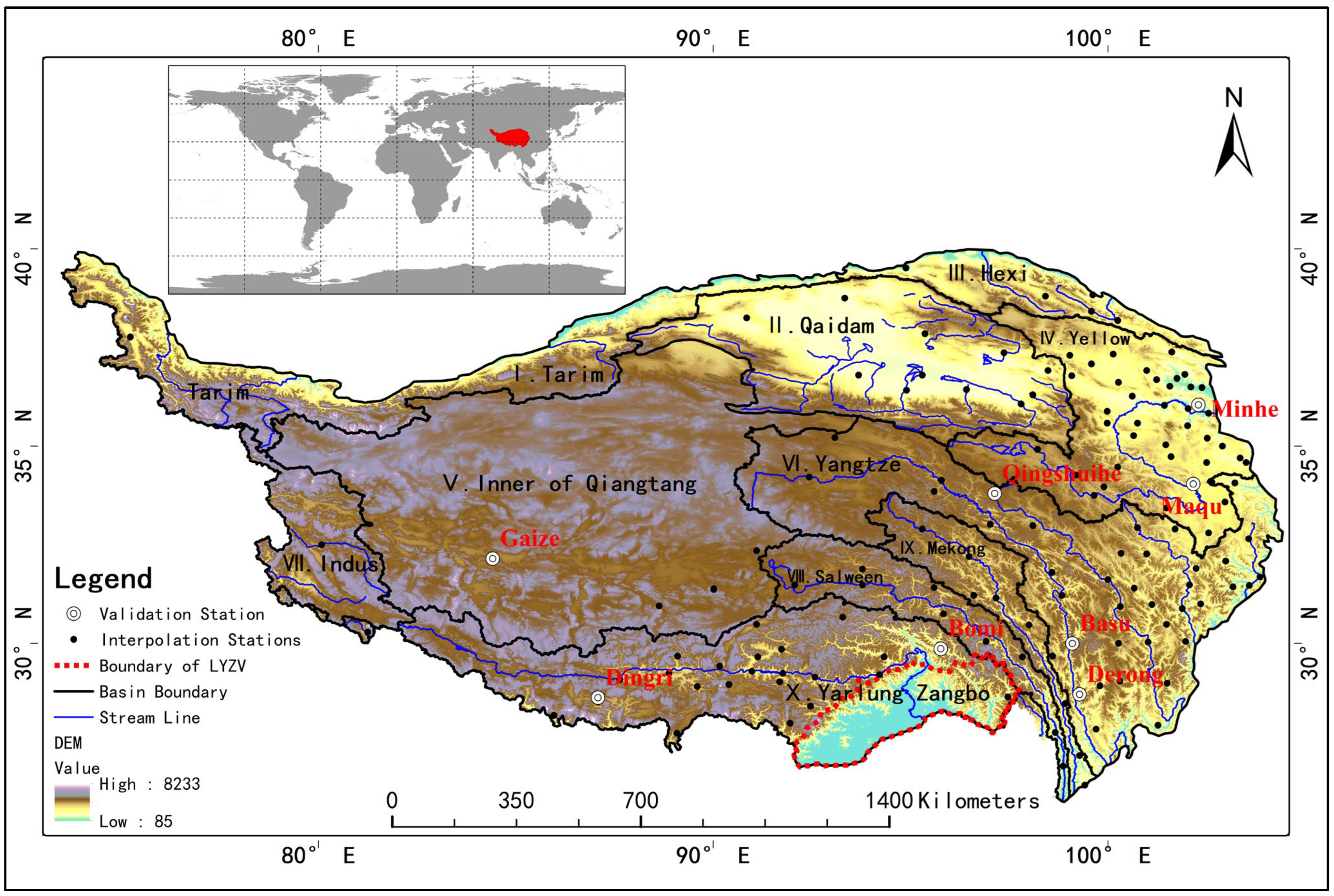
Figure 1. Location and geographical domains for HF-QTP. Black dots and white dots denote the meteorological stations from CMA, white dots are used as verification stations, and black dots are used as interpolation stations in Section 2.6. The QTP’s major river basin boundaries are in black and the main streams are in blue. Due to the absence of surveying and mapping data, the rivers within the Qiangtang region are not depicted on the map. Names of the major river basin boundaries are written within each basin boundary. DEM is shown as the color scale in the background. The boundary of the low Yarlung Zangbo Valley (LYZV) is shown with a red dotted line.
Atmosphere 15 00434 g001
Figure 2. Flowchart for producing historical precipitation data over the QTP based on GPQM and CMFD.
Atmosphere 15 00434 g002
Figure 3. The Q-Q plot between downscaling results and observations from CMA in validation stations. The subfigures are numbered in sequence from (ax) and labeled in the top left corner of each subfigure according to their order. Different colors and dot types denote different downscaling methods. Horizontal axes denote observation values and vertical axes denote downscaling results; they have the same units. The gray dotted line, “x = y”, indicates the 1:1 line. Values closer to this line indicate a more accurate statistical distribution.
Atmosphere 15 00434 g003
Figure 4. Absolute mean bias (AMB) for precipitation (mm d−1) between individual models in CMIP6 and observational data over the QTP, AMB before correction on the left of the blue dotted line (ah), AMB after correction on the right side (ip). The mean value of AMB across the entire QTP is denoted in each subgraph as m; m is defined as the sum of all grid point values divided by the total number of grid points over the Tibetan Plateau, as shown in the following figure. The numbering (I–X) of each subregion (consistent with Figure 1) is also indicated in each subfigure.
Atmosphere 15 00434 g004
Figure 5. AMB is the same as in Figure 4 but for the maximum surface temperature (K).
Atmosphere 15 00434 g005
Figure 6. AMB is the same as in Figure 4 but for minimum surface temperature (K).
Atmosphere 15 00434 g006
Figure 7. The seasonal cycle of precipitation, as well as maximum and minimum temperature, before ((ac), on the left side) and after ((df), on the right side) bias correction. Comparison of the Bayesian model averaging (BMA, blue) mean seasonal cycle of bias-corrected (a,d) precipitation, (b,e) maximum temperature, and (c,f) minimum temperature against the observations for the 1979–2013 period (red). The shaded area represents the uncertainty (from minimum to maximum) of all 7 CMIP6 GCMs.
Atmosphere 15 00434 g007
Figure 8. Future change of precipitation (%) against historical baseline (1985–2010) based on corrected BMA. (ac) The projected change in mean annual precipitation for the SSP1-2.6 in the near (2025–2049), medium (2050–2074), and far (2075–2100) future; (df), (gi) and (jl), the same as (ac) but for SSP2-4.5, SSP3-7.0, and SSP5-8.5, respectively. The mean change across the entire QTP (m) is shown in each panel as m. The numbering of each subregion (consistent with Figure 1) is also indicated in each subfigure. The numbering (I–X) of each subregion (consistent with Figure 1) is also indicated in each subfigure.
Atmosphere 15 00434 g008
Figure 9. Future changes based on BMA; the same as in Figure 8 but for the maximum surface temperature.
Atmosphere 15 00434 g009
Figure 10. Future changes based on BMA; the same as in Figure 8 but for the minimum surface temperature.
Atmosphere 15 00434 g010
Figure 11. Future change time series of BMA and multi-model average (MMA) in precipitation, as well as maximum and minimum temperatures in different subregions (Numbered as (aj), marked in the top left corner of each subfigure) of the QTP. Changes in the BMA and MMA for mean annual precipitation (%), maximum temperature (°C), and minimum temperature (°C) were estimated using a 30-year moving window against the historical reference period of 1979–2013. The shaded region shows uncertainty (estimated using one standard deviation) based on 7 GCMs. Different colors denote the 4 SSPs, and different types of lines denote BMA and MMA, respectively.
Atmosphere 15 00434 g011
Figure 12. Annual mean from 1979 to 2013 (a) and seasonal cycle mean (b) of precipitation from combined data in different subregions of the QTP; the black lines represent the mean values of the QTP, and the colored lines denote multiple subregions.
Atmosphere 15 00434 g012
Figure 13. Signal-to-noise ratio (SNR) of MMA precipitation in different SSPs. The mean values of SNR across the entire QTP are denoted in each subgraph as m. The numbering (I–X) of each subregion (consistent with Figure 1) is also indicated in each subfigure.
Atmosphere 15 00434 g013
Figure 14. SNR, as in Figure 13 but for maximum temperature.
Atmosphere 15 00434 g014
Figure 15. SNR, as in Figure 13 but for minimum temperature.
Atmosphere 15 00434 g015
Table 1. Definition of variables in the HRP-QTP.
VariablesVariable NameUnitPhysical Meaning
PrecipitationPrmm d−1Daily precipitation, both liquid and solid
Maximum temperatureTasmaxKDaily surface (2 m) maximum temperature in one day
Minimum temperatureTasminKDaily surface (2 m) minimum temperature in one day
Table 2. Basic information on verification stations.
NameAltitude (m)Latitude (°)Longitude (°)Year of Initial Observation
Qingshuihe4415.433.8097.131956
Basu2589.230.0099.101952
Derong2422.928.7299.281960
Gaize4414.932.1584.421973
Dingri4300.028.6387.081959
Bomi2736.029.8795.771955
Minhe1813.936.33102.831955
Maqu3471.434.00102.081967
Table 3. Basic information about CMFD and GPQM.
NameResolution (°)Data Time RangeCoverage AreaVariables Used in Present Study
CMFD0.11979–2018Mainland of ChinaPrecipitation rate and temperature
GPQM0.11980–2010A square area covers 70° to 99° east and 25° to 41° northPrecipitation
Table 4. 7 GCMs used in this study.
Modeling GroupModel NameApproximate Grid Spacing (Latitude × Longitude)
Beijing Climate Center (China)BCC-CSM2-MR1.125° × 1.125°
Bjerknes Centre for Climate Research, Norwegian Meteorological Institute (Norway)NorESM2-MM2.5° × 1.875°
Max Planck Institute for Meteorology (Germany)MPI-ESM1-2-HR0.9° × 0.9°
Institute for Numerical Mathematics, Russian Academy of Science (Russia)INM-CM4-81.5° × 2°
Institute Pierre Simon Laplace (France)IPSL-CM6A-LR1.2676° × 2.5°
Meteorological Research Institute, Japan Meteorological Agency (Japan)MRI-ESM2-01.121° × 1.125°
Geophysical Fluid Dynamics Laboratory (America)GFDL-ESM41.25° × 1.00°
Table 5. WD for different methods at 8 independent validation stations. The bold terms indicate the best method for statistical distribution validation.
NameAltitude (m)Pr (mm d−1)Tasmax (K)Tasmin (K)
ANUSPLINIDWOKANUSPLINIDWOKANUSPLINIDWOK
Qingshuihe4415.40.250.820.571.077.695.972.678.687.27
Basu2589.20.551.240.820.418.0513.040.846.599.94
Derong2422.90.691.340.982.378.284.721.968.253.71
Gaize4414.90.241.051.080.393.663.511.465.955.94
Dingri4300.00.561.150.721.80.390.870.783.214.59
Bomi2736.01.051.51.142.863.040.551.234.831.04
Minhe1813.90.390.630.630.393.110.520.664.744.2
Maqu3471.40.150.590.510.151.740.991.50.780.55
Average——0.491.040.811.184.503.771.395.384.66
Table 6. SNRs for precipitation projection results from Cui et al. [30]. The bold terms indicate SNRs greater than 1; SNRs were calculated using Equation (11) ignoring models with no data, and the division of subregions is slightly different from our study.
NameScenariosTemperature Rise Range
1.5 °C2.0 °C3.0 °C
IndusSSP2-4.50.110.351.09
SSP5-8.50.130.100.51
MekongSSP2-4.50.380.241.14
SSP5-8.50.520.330.71
SalweenSSP2-4.50.280.161.32
SSP5-8.50.610.430.80
YangtzeSSP2-4.50.340.790.95
SSP5-8.50.050.380.91
Yarlung ZangboSSP2-4.50.310.260.94
SSP5-8.50.680.380.62
YellowSSP2-4.50.090.561.15
SSP5-8.50.210.140.85
Disclaimer/Publisher’s Note: The statements, opinions and data contained in all publications are solely those of the individual author(s) and contributor(s) and not of MDPI and/or the editor(s). MDPI and/or the editor(s) disclaim responsibility for any injury to people or property resulting from any ideas, methods, instructions or products referred to in the content.