Modification and Validation of the Soil–Snow Module in the INM RAS Climate Model

Abstract

This paper describes the modification of a simple land snow cover module of the INM RAS climate model. The possible liquid water and refreezing of meltwater in the snow layer are taken into account by the proposed parameterization. This is particularly important for modelling the transition season, as this phenomenon is mainly observed during the formation and melting of the snow cover when the surface temperature fluctuates around $0 °$C. The snow density evolution simulation is also added. This parameterization is implemented in the INM-CM snow module and verified on observation data using the ESM-SnowMIP-like protocol. As a result, the INM-CM mean climate snow melt periods are refined, particularly in middle and high latitudes. The snow-covered area according to the model is also improved. In the future, a modified version of the land snow module can be used, coupled with a snow albedo model that takes into account snow metamorphism. This module can also be applied to sea ice snow.

1. Introduction

Simulations using climate models are primary tools for studying climate change. This approach supplements natural observations with numerical experiments, allowing for significant advancements in the study of Earth’s climate. Snow cover has a powerful impact on the climate system, affecting many processes on the Earth.

Seasonal snow cover greatly influences energy balance at the surface (in particular, albedo) [1], the hydrological cycle [2], and other phenomena, for example, winter-time circulation anomalies over mid–high latitudes [3,4].

Snow cover is a complex system controlled by various factors. For example, during transitional seasons with temperature fluctuations around $0 °$C, when the snow melts, not all of the meltwater drains into the soil, but some of its quantity is retained in the snow layer and can be refrozen. These phenomena change the morphology of the snow cover, which can eventually lead to later snowmelt and, thus, affect the hydrological cycle and surface radiation balance. On the other hand, over time, snow becomes denser, absorbs moisture, and can also be contaminated, leading to changes in its optical properties and surface radiation imbalance.

Snow cover models are actively developed both as stand-alone products and as parts of larger projects, such as land surface models (LSMs) or global climate models (GCMs). Verification of snow models takes place in several stages. For example, there are independent model intercomparison projects for land surface (LS3MIP, land surface, snow, and soil moisture model intercomparison project) [5] and snow (ESM-SnowMIP, the Earth system model–snow model intercomparison project) [6] linked to the global climate model comparison project (CMIP6, coupled model intercomparison project–Phase 6) [7,8].

ESM-SnowMIP [6] is an international project that aims to simulate and evaluate modern snow modules integrated into the Earth system models. Within the framework of this project, model data is compared with both local (station) and global observations. One of the objectives is to identify the physical processes that have the greatest impact on the simulation of snow cover features. Another goal is to better assess the Earth system feedback associated with snow in multi-model experiments.

There is a family of global climate models developed at the Marchuk Institute of Numerical Mathematics RAS (INM-CM). This group of models is constantly evolving, and today it includes a set of coupled models with different spatial resolutions, as well as various special modules. Model version INM-CM-48 [9] participates in CMIP6 [7] and shows good results compared to other models [10]. This version includes a soil module with a previous generation of snow cover parameterization. Its description and verification results are given in [11,12]. Future climate change modelling with the INM RAS climate model is discussed in [13], and changes in the Russian Federation are presented in [14]. There is a new version of the INM RAS climate model, INM-CM-60 [15]. This version differs from the previous one, INM-CM-48, with changes in the cloud and condensation scheme, aerosol evolution calculations and their indirect effects, newly implemented land snow and atmospheric boundary-layer parameterizations, and other schemes.

When a new version of any climate model is prepared, it is often not easy to state the reason for climate change from a previous one, because a lot of updates are introduced to it. Here, the response to only one improvement of land snow cover parameterization for the INM RAS climate model is estimated.

This paper proposes a very simple parameterization of snow water refreezing and snow compaction, capable of improving results in single-column simulations proposed in ESM-SnowMIP [6] and as part of the INM RAS Earth system model. The described parameterization is applied to land surface snow only. The new INM-CM snow module is verified against meteorological observations in stand-alone tests and reanalyses, as well as satellite data implemented as part of the INM RAS climate model. It should be noted that the original INM-CM 1D soil module was tested earlier, but the focus was not on snow properties but on surface flows, soil temperature, and freezing depth, which are only indirectly dependent on snow properties [11]. However, here, a direct investigation of snow properties in a single-column mode is presented for both snow parameterization versions. The main novelty of this study is that the implementation of the modified snow parameterization leads to an improvement in the snow simulation in the global climate model.

2. INM-CM Modification

The INM RAS climate model consists of three main modules: atmosphere, ocean, and aerosol dynamics. In this study, the INM-CM-48 [9] version is taken as the base. The spatial resolution of its global atmosphere circulation model is $2°\times 1.5°$ in longitude and latitude and it has 21 vertical $\sigma$ levels. The interactive aerosol module [16], which simulates the evolution of concentrations of 10 substances, is included in the atmosphere model. The ocean global circulation model has a horizontal resolution of $1°\times 0.5°$ in longitude and latitude and 40 vertical $\sigma$ levels. It includes dynamic and thermodynamic modules for the sea ice with elastic–viscous–plastic rheology [17].

2.1. Initial Version of INM-CM Soil–Snow Module

The soil–snow module of the INM-CM family is a part of the atmosphere dynamics model. This one-dimensional module [11,12], describes processes of heat and moisture transfer in soil, vegetation, and snow cover, as well as heat and moisture exchange with the atmosphere. The snow module described here is used as the top layer of the soil–snow module.

The main characteristics of the snow cover are the SWE (snow water equivalent) layer thickness (S, [m]), its density (${\rho }_{sn}$, [kg/${\mathrm{m}}^3$]), and its depth ($H_{sn}$, [m]). In the original version of this module, the SWE calculation is based on the balance equation (Equation (1)), which takes into account snowfall (P—atmospheric precipitation at a negative temperature of underlying surface), snowmelt (M—snowmelt intensity), as well as snow sublimation ($\mathcal{E}$—latent heat flux at the surface spent on snow sublimation, $\mathcal{L}$—specific heat of snow sublimation, ${\rho }_w$–water density).

$${\displaystyle \frac{\mathsf{\partial }S}{\mathsf{\partial }t}}=P-M-{\displaystyle \frac{\mathcal{E}}{\mathcal{L}·{\rho }_w}}$$

(1)

Snow starts to melt when the underlying surface temperature becomes equal to $0 °$C, and the heat balance at the surface is positive. In this scenario, all melted snow, along with any rain that falls on the snow cover, enters the soil immediately. The snowmelt intensity, M, is determined by excess heat flux at the surface, $\mathsf{\Delta }E>0$, and the specific heat of snow melting, $\lambda$ (Equation (2)).

$$M={\displaystyle \frac{\mathsf{\Delta }E}{\lambda }}$$

(2)

In this version, the snow density is assumed to be a constant, i.e., ${\rho }_{sn}=185.4$ kg/${\mathrm{m}}^3$. Note that the snow albedo (${\alpha }_{sn}$) in the INM-CM is determined by a simple parameterization, only depending on the surface temperature, as follows:

$${\alpha }_{sn}=\left\{\begin{array}{c}0.8,T\le -1 °\mathrm{C},\hfill \\ 0.8-0.1·(T+1),T>-1 °\mathrm{C}\hfill \end{array}\right.$$

(3)

2.2. Description of Modified Snow Module in INM-CM

The modification of the INM-CM soil–snow module described here can be divided into several parts: snow melt accumulation processes and changes in snow cover density over time. Firstly, the water equivalent of the snow cover is calculated based on the surface heat balance equation. Then, using the updated amount and composition data of snow cover, the density is updated. Figure 1 shows the conceptual flowchart of the described parameterization.

Snow accumulation–melting processes. The new version of the soil–snow module takes into account the porous structure of the snow layer. It is assumed that water gradually seeps through the snow layer, rather than instantly draining into the soil during snow melt. As the meltwater percolates, it can refreeze and release heat to the surrounding snow. Rainwater is presumed to infiltrate the soil without refreezing.

It is assumed that the amount of liquid water in the snow layer ($S_{wat}$, [m]) cannot exceed a critical value, and any excess water immediately drains into the soil. The critical value of liquid water in snow ($S_{wat}^{max}$) depends on its amount (e.g., SWE) and its porosity (${\epsilon }_{sn}$). These quantities are estimated using the following empirical hydrological formulae [18,19]:

$$S_{wat}^{max}=S·{\displaystyle \frac{{\epsilon }_{sn}}{1-{\epsilon }_{sn}}}$$

(4)

$${\epsilon }_{sn}=0.11·\left({\displaystyle \frac{{\rho }_w}{{\rho }_{sn}}}-1\right)$$

(5)

The consideration of a possible liquid fraction in the snow layer requires the correction of the balance equation for SWE. Firstly, at each time step in the soil–snow module, the surface heat balance is calculated without taking into account possible phase transitions. Then, in the case of phase transitions, possible energy excess in the heat balance, $\mathsf{\Delta }E>0$, is spent on snow melting (as in the original version, the intensity of snow melting is determined by Equation (2)), whereas the energy deficit, $\mathsf{\Delta }E<0$, is spent on the refreezing of meltwater contained in snow pores ($S_{rfrz}$, [m]). The refreezing intensity in this case is determined by the following equation:

$$F=-{\displaystyle \frac{\mathsf{\Delta }E}{\lambda }}$$

(6)

Taking into account the described phenomena, the SWE balance equation is written as follows:

$$\left\{\begin{array}{c}S=S_{atm}+S_{wat}+S_{rfrz},\hfill \\ {\displaystyle \frac{\mathsf{\Delta }S}{\mathsf{\Delta }t}}=P-\widehat{M}+{\displaystyle \frac{\mathsf{\Delta }{S}_{wat}}{\mathsf{\Delta }t}}+{\displaystyle \frac{\mathsf{\Delta }{S}_{rfrz}}{\mathsf{\Delta }t}}-{\displaystyle \frac{\mathcal{E}}{\mathcal{L}·{\rho }_w}}\hfill \end{array}\right.$$

(7)

Here, $S_{atm}$ corresponds to snow in its usual form, falling from the atmosphere as snowflakes, $\widehat{M}=max\left\{0,\left(M-{\displaystyle \frac{S_{wat}^{max}}{\mathsf{\Delta }t}}\right)\right\}$ is the flow of excess meltwater, which is not stored in snow pores and drains into the soil, $\mathsf{\Delta }{S}_{wat}=min\{(M·\mathsf{\Delta }t),S_{wat}^{max}\}$, $\mathsf{\Delta }{S}_{rfrz}=min\{(F·\mathsf{\Delta }t),S_{wat}\}$.

Note that in the modified version, the condition for the onset of melting remains unchanged: the underlying surface temperature is $0 °$C, and the surface heat balance is positive.

Snow density evolution. In the modified version of the INM-CM soil–snow module, the snow cover is represented as a certain substance consisting of four fractions. It can simultaneously include snow in its usual form (both old and freshly fallen) as well as meltwater and refrozen snow. It is important to differentiate fresh and old snow: over time, it becomes denser due to snow grain metamorphism into a more rounded shape, compaction under the weight of over-layers, and refreezing of meltwater [20]. Thus, the density of freshly fallen snow is 50–100 kg/${\mathrm{m}}^3$, and it can reach 500–700 kg/${\mathrm{m}}^3$ for old snow (at the age of 1–2 months).

Snow compaction over time is described with the parameterization, following [21], where there is slow densification under loads resisted by the compactive viscosity:

$${\displaystyle \frac{1}{{\rho }_{sn}}}·{\displaystyle \frac{d{\rho }_{sn}}{dt}}={\displaystyle \frac{M_{sn}·g}{\eta }}$$

(8)

$$\eta ={\eta }_0·exp\left(C_1·(T_C-T_{sn})+C_2·{\rho }_{sn}\right)$$

(9)

Here, ${\rho }_{sn}$ is the snow density, calculated in kg/${\mathrm{m}}^3$, $M_{sn}$ is the snow mass per unit area (in kg/${\mathrm{m}}^2$), $g=10$ m/${\mathrm{s}}^2$ is the acceleration of gravity. The parameter ${\eta }_0$ is the viscosity coefficient at ${\rho }_{sn}=0$ and $T_{sn}=T_C$, $T_{sn}$—snow layer temperature (in K), $T_C=273.2$ K. The constants $C_1$ and $C_2$ equal $0.08$ ${\mathrm{K}}^{-1}$ and 21 ×${10}^{-3}$ ${\mathrm{m}}^3$/kg, respectively.

The Equations (8) and (9) can be rewritten in discrete form as follows:

$${\rho }_{sn}\left(t+\mathsf{\Delta }t\right)={\rho }_{sn}\left(t\right)·\left[1+C_0·\mathsf{\Delta }t·S·exp\left(C_1·t_{sn}^{°}-C_2·{\rho }_{sn}\left(t\right)\right)\right]$$

(10)

Here, S is the SWE in m, $t_{sn}^{°}$ is the snow layer temperature in Celsius, and the value $C_0$ is $0.12$×${10}^{-3}$ 1/(m·s) (this corresponds to ${\eta }_0=8.3$ × ${10}^7$ Pa·s) similar to the SWAP (soil–water–atmosphere–plant) land surface model [18].

Snow that has not fallen during the current model time step is considered to be old. The average snow cover density over the layer, taking into account all four described fractions, is calculated as an SWE-weighted average:

$${\rho }_{snow}={\rho }_{old}·{\delta }_{old}+{\rho }_{new}·{\delta }_{new}+{\rho }_w·{\delta }_{wat}+{\rho }_{ice}·{\delta }_{rfrz}$$

(11)

Here, ${\rho }_{old}$ is the old snow density calculated using the evolutionary model (10), ${\rho }_{new}=100$ kg/${\mathrm{m}}^3$ is freshly fallen snow density, ${\rho }_w=1000$ kg/${\mathrm{m}}^3$ is the water density, ${\rho }_{ice}=917$ kg/${\mathrm{m}}^3$ denotes ice density, ${\delta }_{old},{\delta }_{new},{\delta }_{wat},{\delta }_{rfrz}$ is the ratio (in total water equivalent) of old and fresh snow, meltwater, and refrozen, respectively. The value for fresh snow density is chosen according to the limit of the critical value of liquid water in snow, as follows: $S_{wat}^{max}\ge 0\iff 99.1<{\rho }_{sn}\le 1000$ [kg/${\mathrm{m}}^3$].

3. Verification of INM-CM Soil–Snow Module

To verify the INM-CM soil–snow module, numerical experiments similar to the ESM-SnowMIP project [6] are performed. For this purpose, both local simulations for 10 reference sites (

Table 1. Reference sites used in ESM-SnowMIP [6].

Site	Lat	Lon	Elevation	Start	Finish	Tag	Reference
BERM Old Aspen	$53.63°$	$-106.2°$	600 m	1 October 1997	30 September 2010	OAS	[22]
BERMS Old Black Spruce	$53.99°$	$-105.12°$	629 m	1 October 1997	30 September 2010	OBS	[22]
BERMS Old Jack Pine	$53.92°$	$-104.69°$	579 m	1 October 1997	30 September 2010	OJP	[22]
Col de Porte	$45.3°$	$5.77°$	1325 m	1 October 1994	30 September 2014	CDP	[23]
Reynolds Mountain East	$43.19°$	$-116.78°$	2060 m	1 October 1988	30 September 2008	RME	[24]
Sapporo	$43.08°$	$141.34°$	15 m	1 October 2005	30 September 2015	SAP	[25]
Senator Beck	$37.91°$	$-107.73°$	3714 m	1 October 2005	30 September 2015	SNB	[26]
Sodankyla	$67.37°$	$26.63°$	179 m	1 October 2007	30 September 2014	SOD	[27]
Swamp Angel	$37.91°$	$-107.71°$	3371 m	1 October 2005	30 September 2015	SWA	[26]
Weissfluhjoch	$46.83°$	$9.81°$	2540 m	1 September 1996	31 August 2016	WFJ	[28]

) and global simulations are used. The calculations are conducted with the original version of the INM-CM soil–snow module as well as with the modified version described in this paper. Note that INM-CM is not a contributor to ESM-SnowMIP.

3.1. Local Simulations

For local simulations, observation data from 10 meteorological stations (Table 1) are used. They are located in different regions of the world: alpine, arctic, boreal, and marine regions. For these sites, all necessary data are available [29], for use as input to the model and for evaluating the quality of the simulation. Atmospheric forcings (temperature, pressure, humidity, precipitation, radiation fluxes, wind speed) are used as input data. Snow cover and soil parameters are required as outputs for comparison with observations. In these experiments, the model is run in a single-column mode using only the INM-CM soil–snow module.

3.2. Global Simulations

For the global experiment, simulations were performed using the global climate model INM-CM-48 with original and modified soil–snow modules. An ensemble calculation with 6 runs was carried out for 20 years, starting from a prepared control point on 1 January 1997. The start date and duration of the simulations were chosen as such because observational data on global snow cover have been more reliable since the mid-1990s, as well as due to the available periods of CAMS [30] (2003–2017) and NSIDC-Blended5 [31] (1981–2010) reanalysis data for the comparisons.

For global verification, the spatial distribution of SWE, as well as global metrics, such as the snow-covered area, are used. The simulation results are compared with the results of the ESM-SnowMIP experiments [6], reanalysis data, and observations.

In order to compare the snow-covered area, it is necessary to estimate the snow fraction ratio (SFR) of the model grid cell. For this purpose, the following empirical parameterization [32] is used in the output post-processing stage:

$$SFR=tanh\left({\displaystyle \frac{H_{sn}}{C·{\left({\displaystyle \frac{{\rho }_{sn}}{{\rho }_{new}}}\right)}^{1.6}}}\right)$$

(12)

Here, $H_{sn}$ denotes snow depth (in meters), ${\rho }_{sn}$ and ${\rho }_{new}$ [kg/${\mathrm{m}}^3$] denote current and fresh snow densities, and $C=2.5z_0$, $z_0={10}^{-2}$ m—ground roughness length. Here, the values $2.5$ and $1.6$ are empirical constants according to [33]). The optimal limit value for the SWE of 5 mm is used, corresponding to minimum grid cell coverage [6,34]. If the SWE is less than this value, the snow cover fraction is assumed to be 0.

4. Results

4.1. Local Simulations

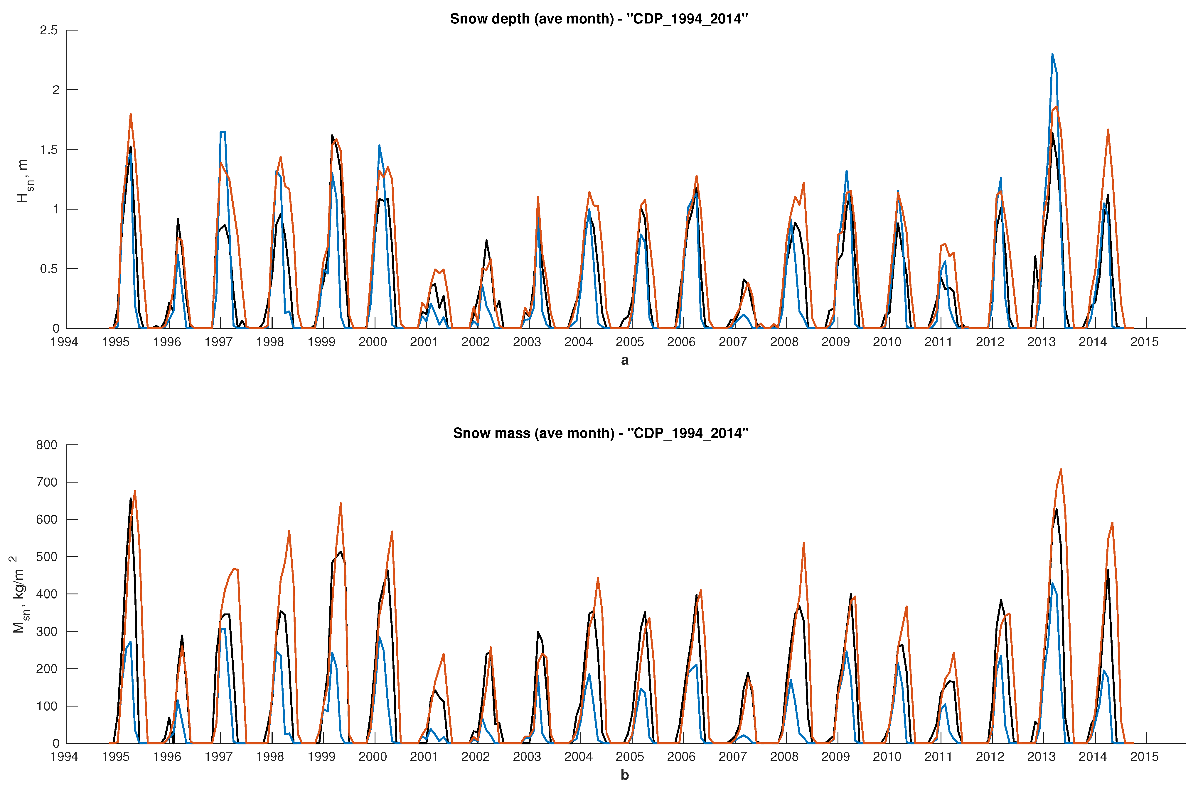
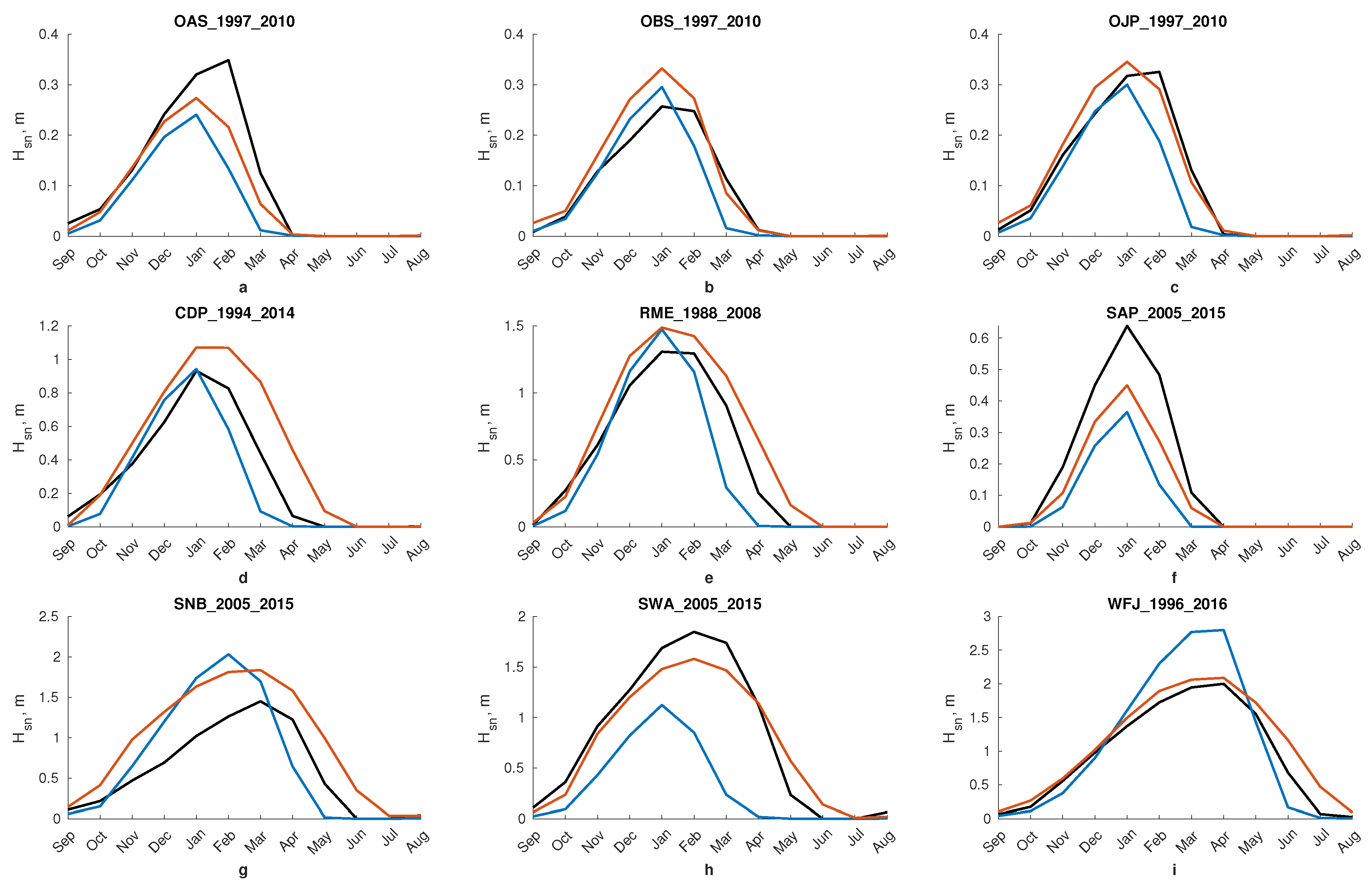
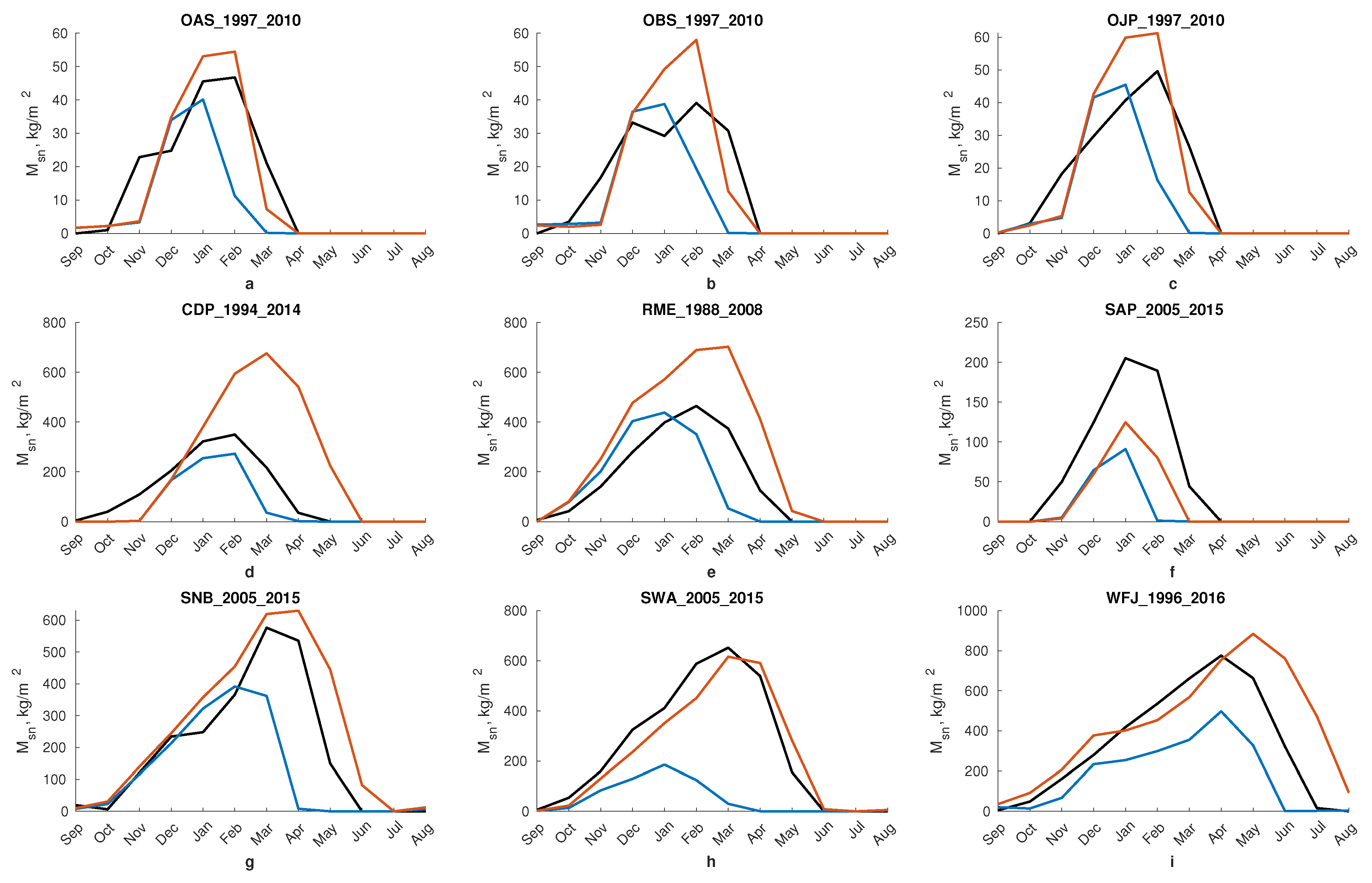
The results of calculations using the soil–snow module of the INM RAS climate model with input data from the ESM-SnowMIP sites show good agreement with the observed data for snow cover and surface and soil temperatures at these stations. Both versions of the snow model (the original INM-CM-48 and the modified one) correctly reproduce the thickness (Figure 2 and Figure 3) and mass (Figure 2 and Figure 4) of the snow cover and the surface temperature (Figure 5). The modified version shows better agreement with observations for the majority of sites, particularly during the spring months when refreezing and changes in snow structure usually occur. According to this version, the snow cover melts an average of 1 month later, which is in agreement with the data from the sites. However, there is an overestimation of the snow amount at some sites. The reasons for this may be the use of a single-layer snow scheme and an overly simple snow albedo parameterization, which leads to slower melting. Nevertheless, as a result of modifications, peak values of SWE and $H_{sn}$ are corrected (most noticeably for the stations Sapporo, Swamp Angel, and Weissfluhjoch), which indicates a more accurate simulation of snow accumulation by the new version of the model. Note that the clarification of modeled snow cover mass is also associated with more accurate modelling of its density, but not only with changes in its depth.

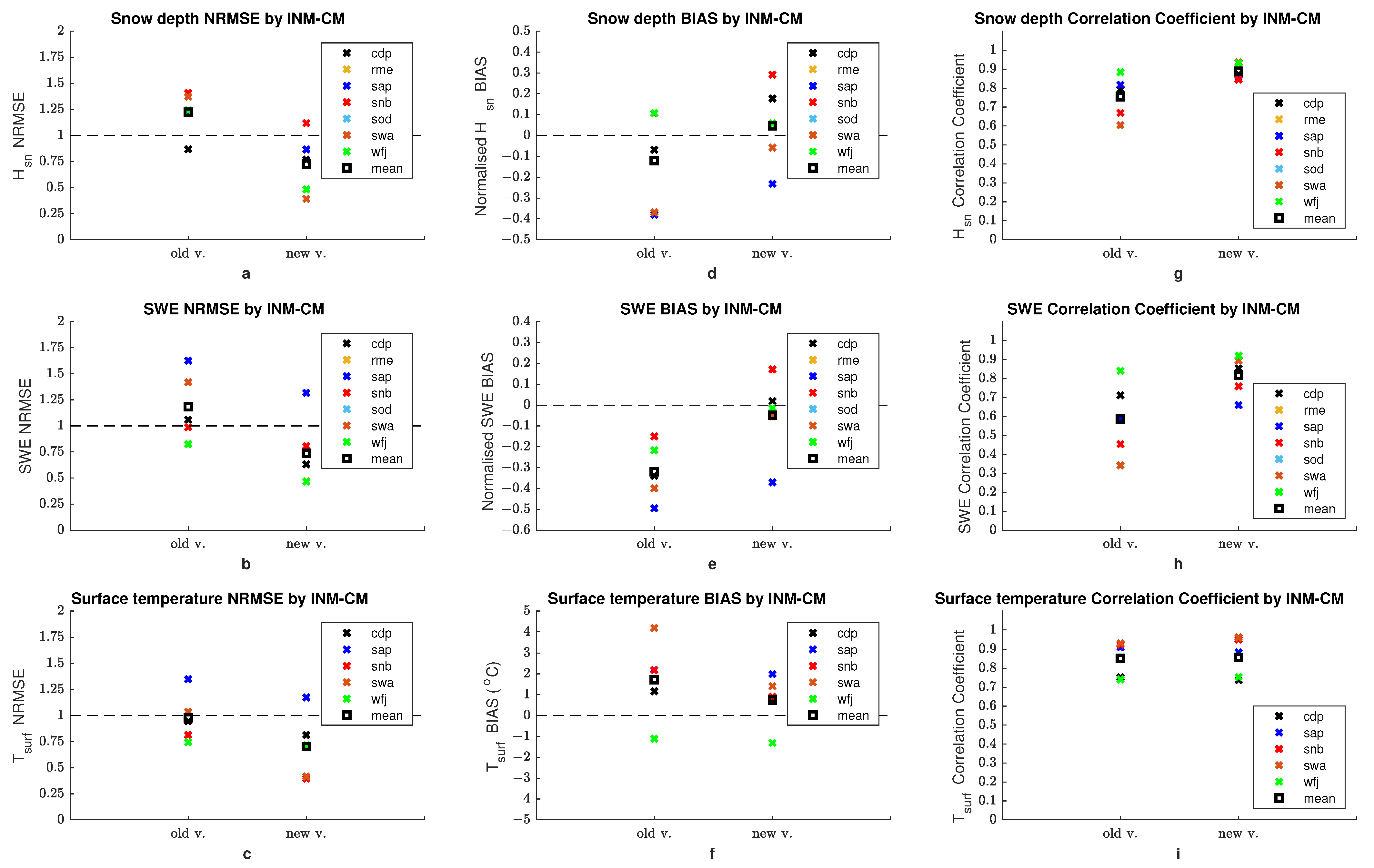
To compare the accuracy of snow cover modelling by the INM-CM and similar models participating in the ESM-SnowMIP project [6,35], basic quality metrics for soil time series data (NRMSE—root mean square error normalized by the standard deviation of observation data, bias, and correlation coefficient) [36] are calculated for the daily height ($H_{sn}$), snow water equivalent (SWE), and surface temperature ($T_{surf}$). Figure 6 shows values for the original and modified versions of the model with respect to observations for available stations, as well as averaged over all such stations. These mean magnitudes are also shown in

Table 2. Quality metrics averaged over stations.

Quality Metrics	INM-CM (Old v.)	INM-CM (New v.)
$H_{sn}$ NRMSE	$1.22$	$0.73$
Normalized $H_{sn}$ bias	$-0.12$	$0.05$
$H_{sn}$ correlation coefficient	$0.82$	$0.91$
SWE NRMSE	$1.18$	$0.73$
Normalized SWE bias	$-0.32$	$-0.05$
SWE correlation coefficient	$0.71$	$0.83$
$T_{surf}$ NRMSE	$0.98$	$0.70$
$T_{surf}$ bias (°C)	$1.72$	$0.74$
$T_{surf}$ correlation coefficient	$0.85$	$0.86$
$T_{soil}$ (at $-0.1$ m) NRMSE	$0.35$	$0.49$
$T_{soil}$ (at $-0.1$ m) bias (°C)	$0.35$	$-0.51$
$T_{soil}$ (at $-0.1$ m) correlation coefficient	$0.96$	$0.86$

. Note that only the days with snow depth greater than $0.1$ m and surface temperature below $0 °$C are included. According to similar plots for snow model errors in [35], the modified version of the INM-CM has an accuracy comparable to other known models.

During testing of the INM-CM soil–snow module, it was noticed that for the mountainous area (stations Col de Porte, Reynolds Mountain East, Senator Beck, Swamp Angel, and Weissfluhjoch), the maximum snow cover strongly differs from the observations, although there is a good agreement on average over the year. To correct this effect, additional model tuning was carried out. Initially, in the INM RAS model, the sensible heat flux between the Earth’s surface and the air $F_{heat}$ was calculated using the following equation [11]:

$$F_{heat}=-{\rho }_a·C_T·V_a·\left({\theta }_a-{\theta }_s\right)$$

(13)

Here, ${\rho }_a$ [kg/${\mathrm{m}}^3$] is the air density at 2 m, $C_T$ is a dimensionless coefficient of heat transfer between the surface and atmosphere, $V_a$ [m/s] is the wind speed module at 2 m, and ${\theta }_a$ and ${\theta }_s$ are the potential temperatures of the air at 2 m and of the surface, respectively. Under typical snowmelt conditions (where the surface temperature is below $0 °$C, the snow temperature is at $0 °$C, and there is stable stratification), $C_T$ is approximately ${10}^{-3}$ or less.

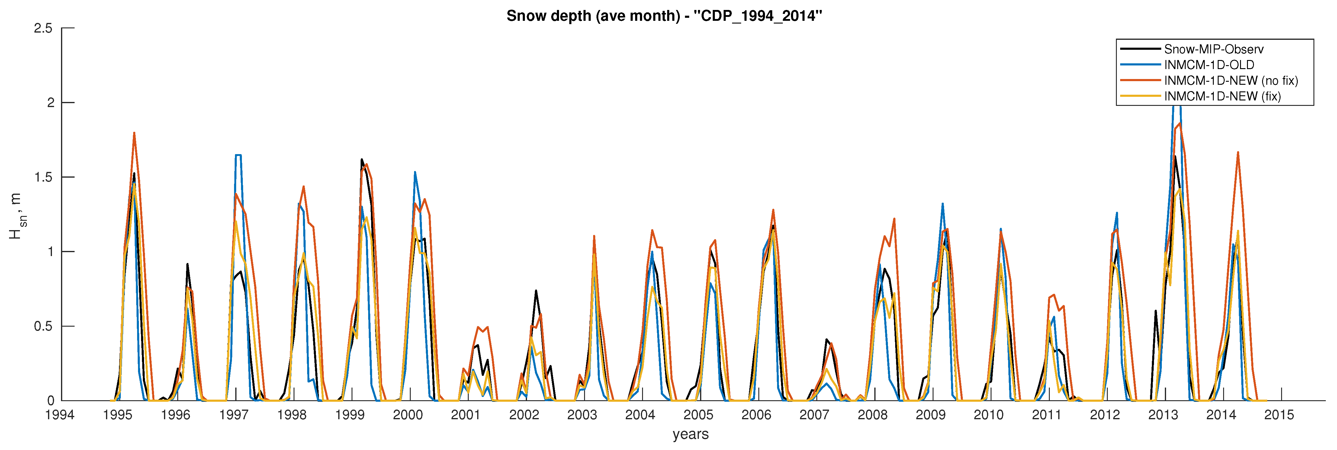
Although the classical Monin–Obukhov theory assumes stable stratification, there is strong turbulence in the mountains, leading to an increased exchange between the surface and atmosphere. Thus, the overestimation of maximum snow cover, as well as the delayed start of melting for stations in the mountains, may be associated with an underestimated sensible heat flux arising from too low of an exchange coefficient. Therefore, for heights over 500 m above sea level, the dimensionless coefficient of heat exchange is bounded from below: $C_T\ge 5$×${10}^{-3}$. As a result, the maximum snow amount is corrected (Figure 7), and the quality value averaged over the snow season is also refined (Figure 8).

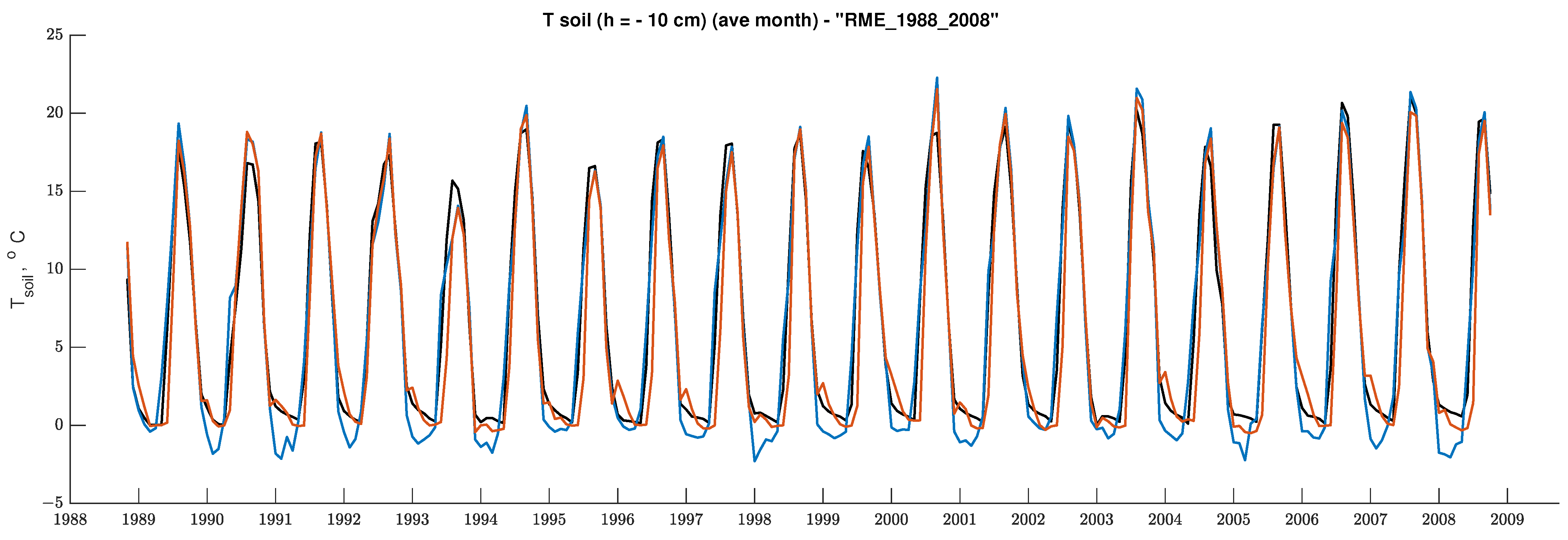
The INM-CM soil–snow module also outputs soil temperature at 23 horizons from 1 cm to 10 m in depth. For most of the stations considered, temperature observation data are available for at least one level within the soil. So, the soil temperature is compared with observations at a depth of 10 cm. There is a strong agreement (Figure 9) with all available site observations for both model versions. Figure 10 shows that the updated snow model does not lead to a sensible decline in the quality of the upper soil layer temperature simulation. However, the positive bias in the soil temperature at 10 cm is changed by a negative one. Snow refreezing in the new version leads to later snowmelt followed by late soil heating in the spring, resulting in an increase in soil water as well as surface latent heat flux during the spring and early summer. Moreover, the correlation coefficient for the temperature of the soil’s top layer decreases from $0.96$ to $0.86$. This may be due to the soil settings specific to the original version of the snow model.

Based on the results of the numerical experiments in the single-column mode, an updated version of the soil–snow module is implemented in the INM RAS global climate model.

4.2. Global Simulations

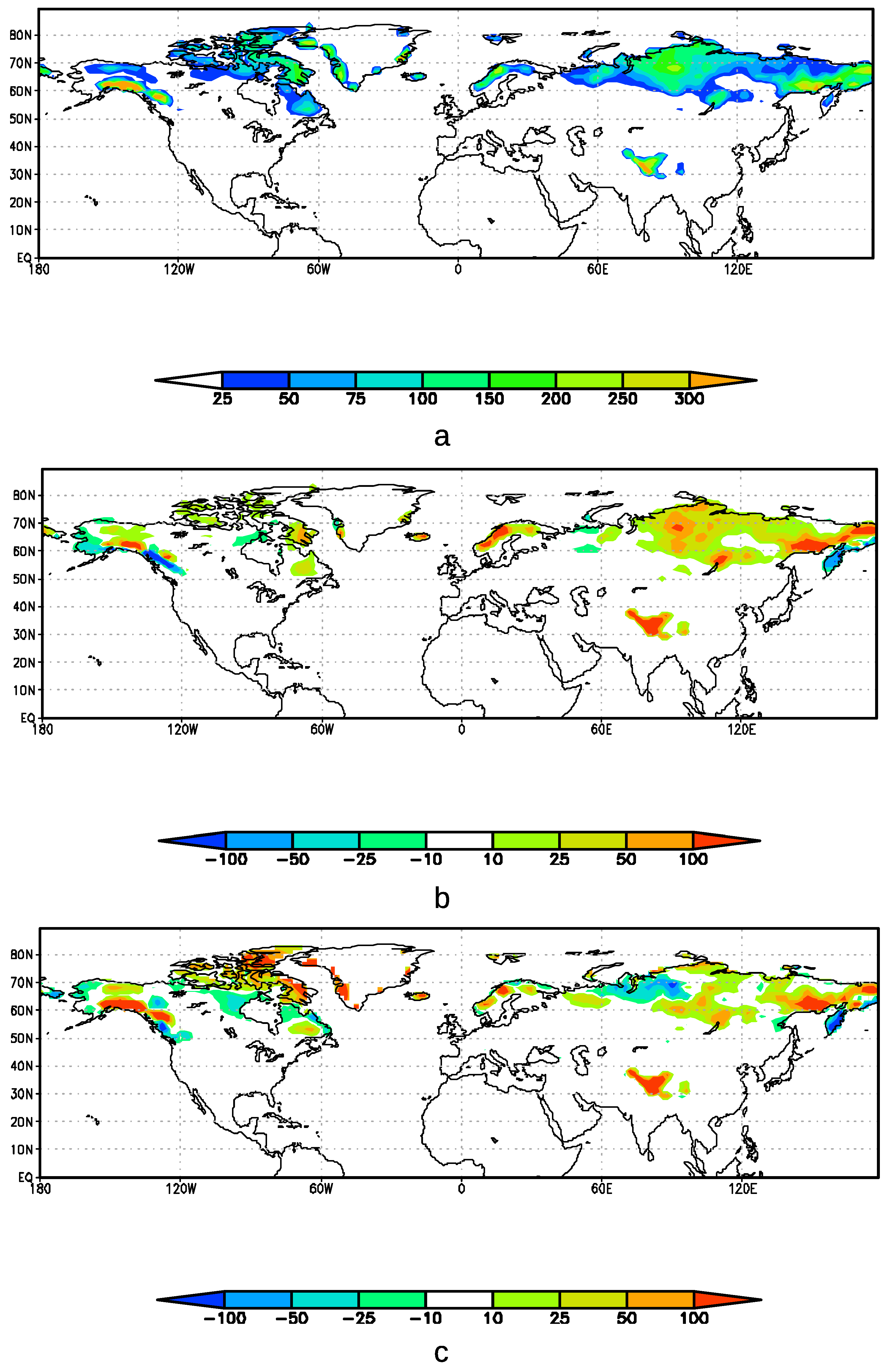
Simulations using the global climate model show results similar to the single column one. The changes in the soil–snow module also lead to later snowmelt (up to a month later in some regions) and more intensive snow cover formation. These effects are especially notable in middle and high latitudes and in the highlands. Now, in the Arctic, as well as in the mountains along the west coast of Canada and Alaska and the Himalayas, snow cover persists into June, whereas in the old version, almost all snow melted in May (Figure 11).

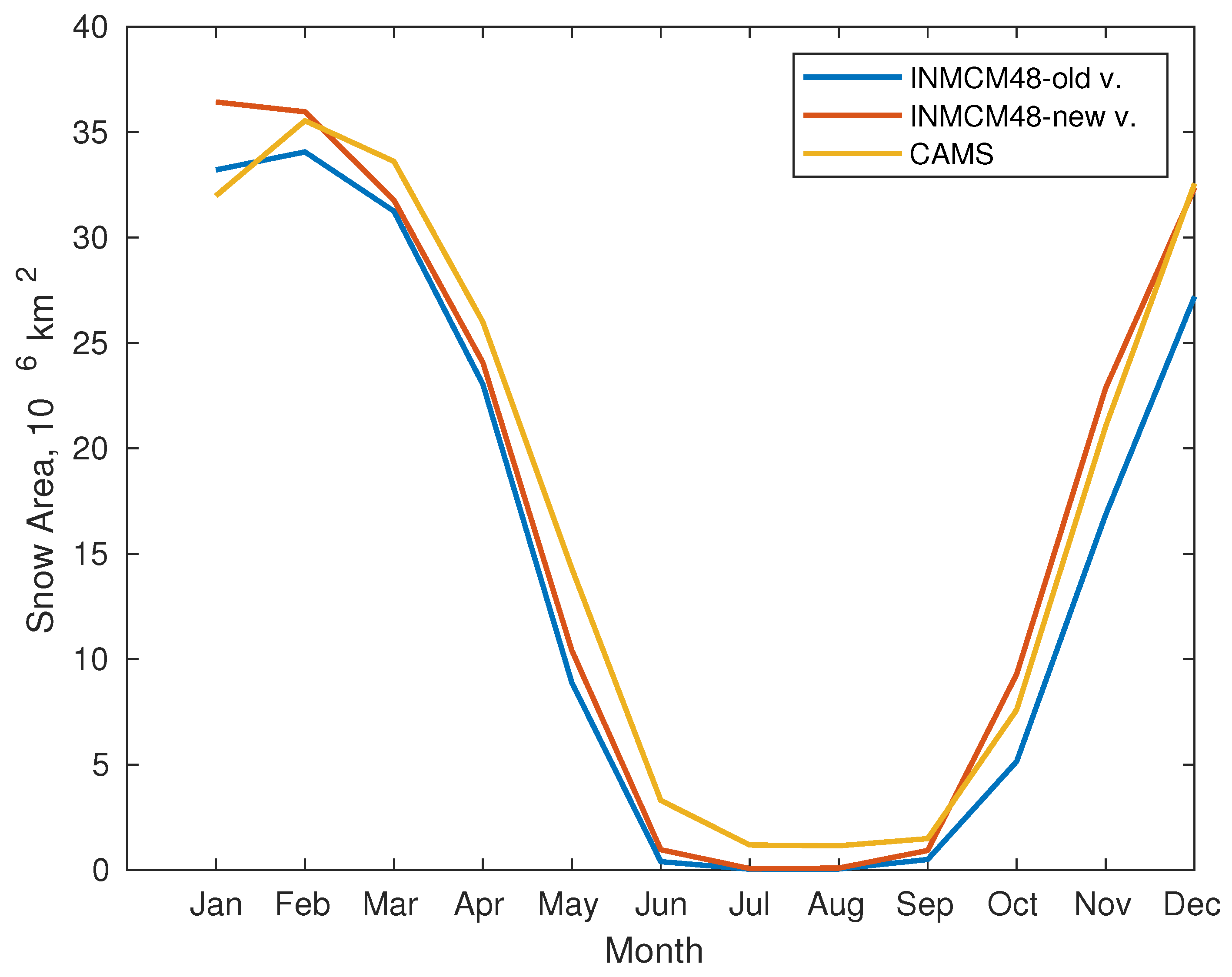
The contribution of the described processes in snow cover formation is also noticeable in late autumn–early winter in the Arctic regions of Eurasia and the Himalayas. These results are consistent with observational data in various regions, e.g., [37]. Figure 12 and Figure 13 show good agreement in the forecasts of snow-covered areas with the CAMS global reanalysis (EAC4) by the European Centre for Medium-Range Weather Forecasts [30] and the NSIDC-Blended5 5-product-based SWE database [31]. The different averaging periods in Figure 12 and Figure 13 are due to the time limits of the available model and reanalysis data.

5. Discussion

The results of the INM-CM soil–snow module are comparable with other snow-covered models. According to the ESM-SnowMIP model ranking by errors [35], the INM RAS climate model version with the new simple snow physics implementation could be placed at about 20th out of 27 models on the quality of SWE simulation. For surface temperature, this version could be ranked between 10th and 12th place out of 27.

In [36], the same soil and surface block [11] was incorporated into the weather forecast model SLAV, and data assimilation results for soil temperature were compared with observations from several groups of European stations. It was found that, in general, the correlation coefficient for the model and observed soil temperature ranged from $0.80$ to $0.95$, while the RMSE was about $0.5$–$1.5$ degrees. This study reports similar correlation coefficient values for the model and observed soil temperatures, with similar or lower RMSE values.

The simulation of SWE and soil temperature in the intermediate complexity climate model IAP RAS is presented in [38,39]. In the IAP RAS model, snow parameterization is similar to the original snow parameterization considered in this study. Detailed parameterization of soil heat and water conductivity is used. In [38], it is shown that the total amount of SWE in their model is simulated reasonably, but the IAP RAS climate model tends to underestimate SWE in Arctic regions and tends to overestimate SWE in middle latitudes, probably due to too simple parameterization of advection of moisture. In this study, the spatial distribution of SWE is simulated better due to the explicit treatment of moisture advection. Also, the IAP RAS climate model tends to overestimate the upper soil temperature in Arctic and Northern Siberia regions, and underestimate the soil temperature in central European Russia, likely because of the simplified treatment of atmospheric advection. The results presented in this study show a better simulation of upper soil temperature because of the explicit treatment of atmosphere dynamics.

Taking into account the different snow layer fractions allows us to describe the snowflake metamorphism, not only for dry but also for wet snow, with the modified version of the model (for example, similar to [40,41]). Snow particle size modelling is one of the approaches used to simulate the snow albedo affecting the radiation balance on the surface. The INM-CM could also take into account the aerosol contamination of snow [42], which is important for the albedo. However, this feature is not currently implemented in the current version of the model. All of these issues could become the subject of future studies that continue the research under discussion.

This study is devoted to snow lying on land, but its results can also be applied to describe sea ice snow with the necessary adjustments. This also accounts for snow blowing and redistribution due to the sea ice movement, puddling, etc.

6. Conclusions

The modified land snow module of the INM RAS climate model is presented. It takes into account the influence of liquid water in the snow and the snow layer densification over time. Here, several well-known parameterizations are used, but their combination may be too new to be incorporated into one snow model.

The land surface module with old and updated snow models was tested in single-column experiments on data from 10 widely scattered sites, covering almost all land areas where snow cover can occur. Snow simulation is improved overall in the modified model, as evidenced by all key metrics for soil modules (except for topsoil temperature) at local sites. The simulation quality of local snow cover data is consistent with the spread of snow models [6], although it is not the best.

The improved version of the snow module was incorporated into the climate model, and long-term global numerical experiments were also carried out. Performed numerical simulations show that the quality of snow cover reproduction is improved with the new version of the INM-CM. As a result, the average climate dates of snow cover melting and the reproduction of a snow-covered surface area, as well as its mass, are improved. Additionally, the updated description of snow layer physics allows for more accurate modelling of related phenomena, such as the radiation balance at the surface.

The main conclusion of this research is that the incorporation of the selected snow parameterization into the climate model leads to improvements in snow simulations in both local and global climate model runs. Furthermore, the presented snow layer parameterization shows results comparable to other models.

References

1. Flanner, M.G.; Shell, K.M.; Barlage, M.; Perovich, D.K.; Tschudi, M.A. Radiative forcing and albedo feedback from the Northern Hemisphere cryosphere between 1979 and 2008. Nat. Geosci. 2011, 4, 151–155. [Google Scholar] [CrossRef]
2. Cohen, J.; Rind, D. The Effect of Snow Cover on the Climate. J. Clim. 1991, 4, 689–706. [Google Scholar] [CrossRef]
3. Cohen, J.; Entekhabi, D. Eurasian snow cover variability and northern hemisphere climate predictability. Geophys. Res. Lett. 1999, 26, 345–348. [Google Scholar] [CrossRef]
4. Cohen, J.; Barlow, M.; Kushner, P.J.; Saito, K. Stratosphere–Troposphere Coupling and Links with Eurasian Land Surface Variability. J. Clim. 2007, 20, 5335–5343. [Google Scholar] [CrossRef]
5. Van den Hurk, B.; Kim, H.; Krinner, G.; Seneviratne, S.I.; Derksen, C.; Oki, T.; Douville, H.; Colin, J.; Ducharne, A.; Cheruy, F.; et al. LS3MIP (v1.0) contribution to CMIP6: The Land Surface, Snow and Soil moisture Model Intercomparison Project—Aims, setup and expected outcome. Geosci. Model Dev. 2016, 9, 2809–2832. [Google Scholar] [CrossRef]
6. Krinner, G.; Derksen, C.; Essery, R.; Flanner, M.; Hagemann, S.; Clark, M.; Hall, A.; Rott, H.; Brutel-Vuilmet, C.; Kim, H.; et al. ESM-SnowMIP: Assessing snow models and quantifying snow-related climate feedbacks. Geosci. Model Dev. 2018, 11, 5027–5049. [Google Scholar] [CrossRef]
7. Eyring, V.; Bony, S.; Meehl, G.A.; Senior, C.A.; Stevens, B.; Stouffer, R.J.; Taylor, K.E. Overview of the Coupled Model Intercomparison Project Phase 6 (CMIP6) experimental design and organization. Geosci. Model Dev. 2016, 9, 1937–1958. [Google Scholar] [CrossRef]
8. Mudryk, L.; Santolaria-Otín, M.; Krinner, G.; Ménégoz, M.; Derksen, C.; Brutel-Vuilmet, C.; Brady, M.; Essery, R. Historical Northern Hemisphere snow cover trends and projected changes in the CMIP6 multi-model ensemble. Cryosphere 2020, 14, 2495–2514. [Google Scholar] [CrossRef]
9. Volodin, E.M.; Mortikov, E.V.; Kostrykin, S.V.; Galin, V.Y.; Lykossov, V.N.; Gritsun, A.S.; Diansky, N.A.; Gusev, A.V.; Iakovlev, N.G.; Shestakova, A.A.; et al. Simulation of the modern climate using the INM-CM48 climate model. Russ. J. Numer. Anal. Math. Model. 2018, 33, 367–374. [Google Scholar] [CrossRef]
10. Kim, Y.H.; Min, S.K.; Zhang, X.; Sillmann, J.; Sandstad, M. Evaluation of the CMIP6 multi-model ensemble for climate extreme indices. Weather Clim. Extrem. 2020, 29, 100269. [Google Scholar] [CrossRef]
11. Volodin, E.; Lykossov, V. Parameterization of Heat and Moisture Transfer in the Soil-Vegetation System for Use in Atmospheric General Circulation Models: 1. Formulation and Simulations Based on Local Observational Data. Izv. Atmos. Ocean. Phys. 1998, 34, 405–416. [Google Scholar]
12. Volodina, E.E.; Bengtsson, L.; Lykossov, V. Parametrization of heat and water transfer through snowpack for simulation of seasonal variability of hydrological land parameters. Meteorol. Hydrol. 2000, 10, 1–8. [Google Scholar]
13. Volodin, E.M.; Gritsun, A.S. Simulation of Possible Future Climate Changes in the 21st Century in the INM-CM5 Climate Model. Izv. Atmos. Ocean. Phys. 2020, 56, 218–228. [Google Scholar] [CrossRef]
14. Volodin, E.M. Possible Climate Change in Russia in the 21st Century Based on the INM-CM5-0 Climate Model. Russ. Meteorol. Hydrol. 2022, 47, 327–333. [Google Scholar] [CrossRef]
15. Volodin, E.M. Simulation of Present-Day Climate with the INMCM60 Model. Izv. Atmos. Ocean. Phys. 2023, 59, 16–22. [Google Scholar] [CrossRef]
16. Volodin, E.M.; Kostrykin, S.V. The aerosol module in the INM RAS climate model. Russ. Meteorol. Hydrol. 2016, 41, 519–528. [Google Scholar] [CrossRef]
17. Yakovlev, N.G. Reproduction of the large-scale state of water and sea ice in the Arctic Ocean in 1948–2002: Part 1. Numerical model. Izv. Atmos. Ocean. Phys. 2009, 45, 357–371. [Google Scholar] [CrossRef]
18. Gusev, Y.M.; Nasonova, O.N. The simulation of heat and water exchange at the land–atmosphere interface for the boreal grassland by the land-surface model SWAP. Hydrol. Process. 2002, 16, 1893–1919. [Google Scholar] [CrossRef]
19. Kuchment, L.S.; Demidov, V.N.; Motovilov, Y.G. Formirovanie rechnogo stoka: Fisiko-matematicheskie modeli (River Runoff Formation: Physically Based Models); Nauka: Moscow, Soviet Union, 1983. (In Russian) [Google Scholar]
20. Essery, R.; Morin, S.; Lejeune, Y.; B Ménard, C. A comparison of 1701 snow models using observations from an alpine site. Adv. Water Resour. 2013, 55, 131–148. [Google Scholar] [CrossRef]
21. Anderson, E.A. A Point Energy and Mass Balance Model of a Snow Cover; NOAA Technical Report NWS 19; Stanford University: Stanford, CA, USA, 1976. [Google Scholar]
22. Bartlett, P.A.; MacKay, M.D.; Verseghy, D.L. Modified snow algorithms in the Canadian land surface scheme: Model runs and sensitivity analysis at three boreal forest stands. Atmosphere-Ocean 2006, 44, 207–222. [Google Scholar] [CrossRef]
23. Lejeune, Y.; Dumont, M.; Panel, J.M.; Lafaysse, M.; Lapalus, P.; Le Gac, E.; Lesaffre, B.; Morin, S. 57 years (1960–2017) of snow and meteorological observations from a mid-altitude mountain site (Col de Porte, France, 1325 m of altitude). Earth Syst. Sci. Data 2019, 11, 71–88. [Google Scholar] [CrossRef]
24. Reba, M.L.; Marks, D.; Seyfried, M.; Winstral, A.; Kumar, M.; Flerchinger, G. A long-term data set for hydrologic modeling in a snow-dominated mountain catchment. Water Resour. Res. 2011, 47, W07702. [Google Scholar] [CrossRef]
25. Niwano, M.; Aoki, T.; Kuchiki, K.; Hosaka, M.; Kodama, Y. Snow Metamorphism and Albedo Process (SMAP) model for climate studies: Model validation using meteorological and snow impurity data measured at Sapporo, Japan. J. Geophys. Res. Earth Surf. 2012, 117, F03008. [Google Scholar] [CrossRef]
26. Landry, C.C.; Buck, K.A.; Raleigh, M.S.; Clark, M.P. Mountain system monitoring at Senator Beck Basin, San Juan Mountains, Colorado: A new integrative data source to develop and evaluate models of snow and hydrologic processes. Water Resour. Res. 2014, 50, 1773–1788. [Google Scholar] [CrossRef]
27. Essery, R.; Kontu, A.; Lemmetyinen, J.; Dumont, M.; Ménard, C.B. A 7-year dataset for driving and evaluating snow models at an Arctic site (Sodankylä, Finland). Geosci. Instrum. Methods Data Syst. 2016, 5, 219–227. [Google Scholar] [CrossRef]
28. Wever, N. Weissfluhjoch Dataset for ESM-SnowMIP. 2017. Available online: https://envidat.ch/#/metadata/snowmip (accessed on 15 December 2023). [CrossRef]
29. Ménard, C.B.; Essery, R.; Barr, A.; Bartlett, P.; Derry, J.; Dumont, M.; Fierz, C.; Kim, H.; Kontu, A.; Lejeune, Y.; et al. Meteorological and evaluation datasets for snow modelling at 10 reference sites: Description of in situ and bias-corrected reanalysis data. Earth Syst. Sci. Data 2019, 11, 865–880. [Google Scholar] [CrossRef]
30. Inness, A.; Ades, M.; Agustí-Panareda, A.; Barré, J.; Benedictow, A.; Blechschmidt, A.; Dominguez, J.; Engelen, R.; Eskes, H.; Flemming, J.; et al. CAMS Global Reanalysis (EAC4) Monthly Averaged Fields. 2019. Available online: https://www.copernicus.eu/en/access-data/copernicus-services-catalogue/cams-global-reanalysis-eac4 (accessed on 30 September 2021).
31. Mudryk, L.R.; Derksen, C. CanSISE Observation-Based Ensemble of Northern Hemisphere Terrestrial Snow Water Equivalent, Version 2. 2017. Available online: https://nsidc.org/data/nsidc-0668/versions/2 (accessed on 29 September 2021). [CrossRef]
32. Niu, G.Y.; Yang, Z.L. An observation-based formulation of snow cover fraction and its evaluation over large North American river basins. J. Geophys. Res. Atmos. 2007, 112. [Google Scholar] [CrossRef]
33. Swenson, S.C.; Lawrence, D.M. A new fractional snow-covered area parameterization for the Community Land Model and its effect on the surface energy balance. J. Geophys. Res. Atmos. 2012, 117. [Google Scholar] [CrossRef]
34. Robinson, D.A.; Hall, D.K.; Mote, T.L. PMEaSUREs Northern Hemisphere Terrestrial Snow Cover Extent Daily 25 km EASE-Grid 2.0, Version 1; NASA National Snow and Ice Data Center Distributed Active Archive Center: Boulder, CO, USA, 2014; Available online: https://nsidc.org/data/nsidc-0530/versions/1 (accessed on 10 October 2021). [CrossRef]
35. Menard, C.B.; Essery, R.; Krinner, G.; Arduini, G.; Bartlett, P.; Boone, A.; Brutel-Vuilmet, C.; Burke, E.; Cuntz, M.; Dai, Y.; et al. Scientific and Human Errors in a Snow Model Intercomparison. Bull. Am. Meteorol. Soc. 2021, 102, E61–E79. [Google Scholar] [CrossRef]
36. Travova, S.V.; Stepanenko, V.M.; Medvedev, A.I.; Tolstykh, M.A.; Bogomolov, V.Y. Quality of Soil Simulation by the INM RAS–MSU Soil Scheme as a Part of the SL-AV Weather Prediction Model. Russ. Meteorol. Hydrol. 2022, 47, 159–173. [Google Scholar] [CrossRef]
37. Robinson, D.A.; Estilow, T.W.; NOAA Climate Data Record Program. NOAA Climate Data Record (CDR) of Northern Hemisphere (NH) Snow Cover Extent (SCE), Version 1; NOAA National Centers for Environmental Information: Asheville, NC, USA, 2014. Available online: https://www.ncei.noaa.gov/access/metadata/landing-page/bin/iso?id=gov.noaa.ncdc:C00756 (accessed on 30 November 2023). [CrossRef]
38. Arzhanov, M.M.; Demchenko, P.F.; Eliseev, A.V.; Mokhov, I.I. Simulation of characteristics of thermal and hydrologic soil regimes in equilibrium numerical experiments with a climate model of intermediate complexity. Izv. Atmos. Ocean. Phys. 2008, 44, 548–566. [Google Scholar] [CrossRef]
39. Eliseev, A.V.; Mokhov, I.I.; Arzhanov, M.M.; Demchenko, P.F.; Denisov, S.N. Interaction of the methane cycle and processes in wetland ecosystems in a climate model of intermediate complexity. Izv. Atmos. Ocean. Phys. 2008, 44, 139–152. [Google Scholar] [CrossRef]
40. Flanner, M.G.; Zender, C.S.; Randerson, J.T.; Rasch, P.J. Present-day climate forcing and response from black carbon in snow. J. Geophys. Res. Atmos. 2007, 112. [Google Scholar] [CrossRef]
41. Brun, E. Investigation on Wet-Snow Metamorphism in Respect of Liquid-Water Content. Ann. Glaciol. 1989, 13, 22–26. [Google Scholar] [CrossRef]
42. Chernenkov, A.Y.; Kostrykin, S.V. Estimation of Radiative Forcing from Snow Darkening with Black Carbon Using Climate Model Data. Izv. Atmos. Ocean. Phys. 2021, 57, 133–141. [Google Scholar] [CrossRef]
43. Menard, C.; Essery, R. ESM-SnowMIP meteorological and evaluation datasets at ten reference sites (in situ and bias corrected reanalysis data). Pangaea 2019. [Google Scholar] [CrossRef]
44. Chernenkov, A.; Volodin, E.; Kostrykin, S.; Tarasevich, M.; Vorobyeva, V. Modification and Verification of Soil-Snow Module of INM RAS Climate Model. 2023. Available online: https://b2share.eudat.eu (accessed on 15 December 2023). [CrossRef]
Figure 1. Conceptual flowchart of the modified snow model.
Atmosphere 15 00422 g001
Figure 2. Monthly average depth (a) and mass (b) of snow cover during the entire simulation period for the Col de Porte site, according to the INM-CM snow module (blue—original version, red—modified) and observations (black).
Atmosphere 15 00422 g002
Figure 3. Annual variation of snow depths averaged over the simulation period, according to the INM-CM snow module (blue—original version, red—modified) and site observations (black).
Atmosphere 15 00422 g003
Figure 4. Annual variation of snow mass averaged over the simulation period, according to the INM-CM snow module (blue—original version, red—modified) and site observations (black).
Atmosphere 15 00422 g004
Figure 5. Monthly average surface temperatures for Col de Porte (a), Swamp Angel (b), and Weissfluhjoch (c) sites during the entire simulation period, according to the INM-CM snow module (blue—original version, red—modified) and observations (black).
Atmosphere 15 00422 g005
Figure 6. Quality metrics (normalized root-mean-square errors, bias, and correlation coefficient) for snow depth, snow water equivalent thickness, and surface temperature.
Atmosphere 15 00422 g006
Figure 7. Monthly average snow depth during the simulation period for the Col de Porte site, according to the different INM-CM snow module versions (including the version with the correction of the heat transfer coefficient, C T ) and observation data.
Atmosphere 15 00422 g007
Figure 8. Quality metrics (normalized root-mean-square errors, bias, and correlation coefficient) for snow depth and SWE for mountain sites (for the original, modified, and modified with the additional tuning of the INM-CM snow module versions).
Atmosphere 15 00422 g008
Figure 9. Monthly average soil temperature at a depth of 10 cm during the simulation period for the Reynolds Mountain East site, according to the INM-CM snow module (blue—original version, red—modified) and observations (black).
Atmosphere 15 00422 g009
Figure 10. Quality metrics (normalized root-mean-square errors, bias, and correlation coefficient) for the temperature in the upper soil layers (at a depth of ∼10 cm) according to the different INM-CM snow module versions.
Atmosphere 15 00422 g010
Figure 11. (a) Mean monthly SWE according to the INM RAS global climate model with the modified version of the soil–snow module, (b) difference with the original version (INM-CM48), and (c) with the NSIDC-Blended5 reanalysis data (in [mm]; model data averaged over the ensemble and all simulation period; month—May).
Atmosphere 15 00422 g011
Figure 12. Annual snow-covered area variation in the Northern Hemisphere (averaged over the ensemble and for 2003–2017) according to the original and modified versions of INM-CM and CAMS reanalysis data.
Atmosphere 15 00422 g012
Figure 13. Annual snow-covered area variation in the Northern Hemisphere (averaged over the ensemble and for 1998–2010) according to the original and modified versions of INM-CM and the NSIDC-Blended5 reanalysis data.
Atmosphere 15 00422 g013