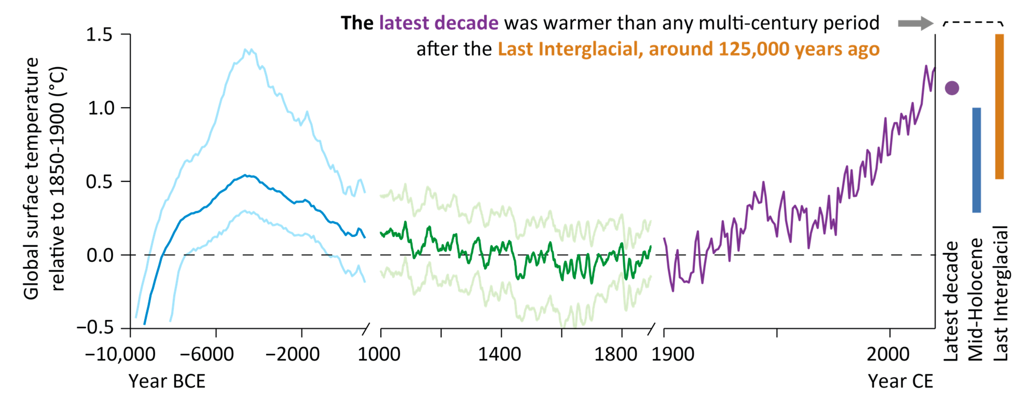
Is Recent Warming Exceeding the Range of the Past 125,000 Years?

Abstract

The Intergovernmental Panel on Climate Change (IPCC) concluded that the latest decade was warmer than any multi-century period over the past 125,000 years. This statement rests on a comparison of modern instrumental measurements against the course of past temperatures reconstructed from natural proxy archives, such as lake and marine sediments, and peat bogs. Here, we evaluate this comparison with a focus on the hundreds of proxy records developed by paleoclimatologists across the globe to reconstruct climate variability over the Holocene (12,000 years) and preceded by the Last Glacial Period (125,000 years). Although the existing proxy data provide a unique opportunity to reconstruct low-frequency climate variability on centennial timescales, they lack temporal resolution and dating precision for contextualizing the most recent temperature extremes. While the IPCC’s conclusion on the uniqueness of latest-decade warming is thus not supported by comparison with these smoothed paleotemperatures, it is still likely correct as ice core-derived forcing timeseries show that greenhouse gases were not elevated during any pre-instrumental period of the Holocene.

1. Background and Motivation

Working Group 1 of the Intergovernmental Panel on Climate Change [1] included a figure in their Technical Summary showing a comparison of (i) instrumental global surface temperatures (GSTs) since 1900 CE with (ii) a high-resolution, mostly tree-ring-based, GST reconstruction from 1000 to 1900 CE, and (iii) a smoothed proxy-based GST reconstruction from 10,000 BCE to 1000 CE (Figure 1). The figure illustrates that the instrumental GSTs recorded over the last decade from 2011 to 2020 CE exceeded the range of proxy-reconstructed GSTs during the mid-Holocene culminating at roughly 4500 BCE. The latter represents the so-called Holocene Optimum (HOP) during which GSTs were elevated in response to increased orbital forcing [2,3]. Since the HOP was preceded by the Last Glacial Period and followed by a long-term cooling trend culminating in the 15th-to-19th century Little Ice Age (see the green curve in Figure 1), the IPCC figure included a statement saying that the latest decade was warmer than any multi-century period over the past 125,000 years. The likelihood of this statement is described to be “more likely than not”, which translates to a level of confidence range from >50 to 100%.

The figure included in the IPCC report founded the basis for a public discourse on record-breaking warmth, such as the 4th of July that was described as the hottest day, and the 3rd to 10th of July as the hottest week in over 100,000 years [4,5]. While it is without question that these extremes are forced by greenhouse gases, and accelerated by an impending El Niño, it remains unclear why the IPCC related a single decade with a multi-century period and, more generally, how meaningful such comparisons including different temporal scales are. Here, we address these questions by reviewing some of the key characteristics of the underlying proxy data used to reconstruct GST back to 10,000 BCE. Our assessment focusses on the spatial coverage, data replication, and temporal resolution of the global Holocene proxy network, with the aim to provide guidance for the possibilities and limitations of contextualizing recent extremes with pre-Anthropocene climate variability.

Figure 1. Recorded and reconstructed GSTs since 10,000 BCE from the IPCC AR6 Technical Summary (p. 61) [1]. The purple curve shows instrumental temperatures recorded since 1900 CE at annual resolution (HadCRUT 5) [6]. The green and blue curves are temperature reconstructions derived from multiple proxies from 1000 to1900 CE and 10,000 BCE to 1000 CE at decadal and centennial resolutions, respectively [7,8]. The light color curves are uncertainty estimates. All temperatures are shown as anomalies from an 1850–1900 CE reference period.

Figure 1. Recorded and reconstructed GSTs since 10,000 BCE from the IPCC AR6 Technical Summary (p. 61) [1]. The purple curve shows instrumental temperatures recorded since 1900 CE at annual resolution (HadCRUT 5) [6]. The green and blue curves are temperature reconstructions derived from multiple proxies from 1000 to1900 CE and 10,000 BCE to 1000 CE at decadal and centennial resolutions, respectively [7,8]. The light color curves are uncertainty estimates. All temperatures are shown as anomalies from an 1850–1900 CE reference period.

2. Data Sources and Methods

2.1. Instrumental and Proxy Data in the IPCC Figure

The instrumental data shown in the IPCC figure (Figure 1) combine terrestrial surface air temperatures measured in white boxes ~2 m above ground with sea surface temperatures measured in the upper few meters of the ocean water column. Whereas the daily measurement procedures, instruments, and numbers of data points varied dramatically over the past 120 years [6,9,10], the displayed GST trend from thousands of locations across the globe is highly accurate and demonstrates a greenhouse gas-forced temperature increase of >1 °C. This instrumental period since 1900 CE is preceded by a warm-season-weighted temperature reconstruction back to 1000 CE, mainly from annually resolved tree-ring data that were smoothed here to emphasize decadal-scale variability. This record (shown in green in Figure 1) is in line with previous large-scale reconstructions revealing warmer conditions during medieval times followed by a cooling trend into the Little Ice Age culminating in the 15th–19th centuries [11,12,13]. Prior to 1000 CE, the proxies display ~0.5 °C warmer conditions during the HOP centered around 4500 BCE and preceded by much colder GSTs at the transition from the Last Glacial Period to the Holocene (the blue curve in Figure 1). A comparison of mid-Holocene conditions with GSTs recorded from 2011 to 2020 (see the bars and symbols on the right side of Figure 1) indicates the latest decade to fall outside the range of temperature variability since the Last Interglacial 125,000 years ago.

2.2. Holocene Proxy Network

The Holocene GST record displayed in the Technical Summary is composed of a total of 1319 proxy records from 679 sites across the globe (Figure 2). The proxy locations are heavily weighted towards the Northern Hemisphere as the network’s latitudinal mean is situated at 46.7° N, challenging the representation of the Tropics and Southern Hemisphere. This bias is mitigated back in time as the network mean gradually shifts from 50° N towards 15° N before 5500 BCE when several shorter proxy records drop out. The majority of proxies used in the Holocene network are from lake sediments (54%), followed by marine sediments (27%), peat bogs (15%), and other archives (4%). A proportion of 46% of the proxies are described to represent annual mean temperatures, 34% summer temperatures, and 20% winter temperatures, though it is important to bear boreal and austral summers in mind when aggregating such data [14,15,16,17].

2.3. Single Proxy Records

The proxy records included in the global network have been developed by dozens of research teams over several decades and are the result of hundreds of field, measurement, and analysis campaigns. They form the backbone of any empirical assessment of Holocene climate variability and serve as a blueprint for climate modeling [18]. Each temperature record from these campaigns, whether derived from pollen assemblages, stable isotopes, alkenone, chironomids, or otherwise, represents an individual timeseries with singular characteristics. To value this variety, we display here 6 of the 1319 proxy records used in the IPCC report in their original units in °C to emphasize individual differences in variance, resolution, and seasonality (Figure 3).

The tree-ring chronology from northern Finland (top panel in Figure 3) represents one of the most highly resolved proxies of the network; yet, the reconstructed summer temperature variability is confined to the low-frequency domain as the necessary dendrochronological detrending removed any long-term trend from the data [19]. Such records can therefore not contribute to the long-term temperature evolution throughout the Holocene but attenuate the network mean towards zero. The second record, a pollen-based temperature reconstruction from a lake in Spain, matches the average resolution of all 1319 records included in the Holocene network (165 years). The temporally increasing spacing between data points back in time—from more data points in the second millennium CE to only a few points before 1000 BCE—is characteristic to many Holocene proxies. Finally, the δ¹⁸O record from the Brazilian margin represents a proxy from the lower end of the resolution spectrum including a data point only every 640 years. Such low-resolution records are primarily considered in the Southern Hemisphere and Tropics to mitigate effects of low sample replication in these areas.

Figure 3. Varying resolution and seasonality among individual proxy records. (a) Annually resolved (1-year resolution) summer temperature reconstruction from a northern Finland tree-ring width chronology [20], shown together with a medium-resolution (167 years) annual temperature reconstruction from pollen assemblages of a 206 cm lake core from Spain [21], and a low-resolution (640 years) annual temperature reconstruction from δ¹⁸O isotopes of a 208 cm marine core from coastal Brazil [22]. (b) Top curves show a summer and winter temperature reconstruction from pollen compositions of a 723 cm lake core in Switzerland [23]. Bottom panel shows the annual temperature timeseries derived from averaging the summer and winter reconstructions.

Figure 3. Varying resolution and seasonality among individual proxy records. (a) Annually resolved (1-year resolution) summer temperature reconstruction from a northern Finland tree-ring width chronology [20], shown together with a medium-resolution (167 years) annual temperature reconstruction from pollen assemblages of a 206 cm lake core from Spain [21], and a low-resolution (640 years) annual temperature reconstruction from δ¹⁸O isotopes of a 208 cm marine core from coastal Brazil [22]. (b) Top curves show a summer and winter temperature reconstruction from pollen compositions of a 723 cm lake core in Switzerland [23]. Bottom panel shows the annual temperature timeseries derived from averaging the summer and winter reconstructions.

The other example (Figure 3b) illustrates how an annual temperature record is produced by simply averaging two seasonal timeseries, in this case, a pollen-derived summer and a winter temperature record from a lake in Switzerland. Whereas the summer record has a mean of ~18.5 °C and includes a modest long-term warming trend, the winter record is much colder (~0.5 °C) and characterized by a long-term cooling trend. Averaging these records attenuates these features and produces a timeseries with a temperature mean at ~9.5 °C. This procedure of producing annual temperature records, when both a summer and a winter proxy are available at a single site, is regularly conducted in the global network (43% of all annual records) and massively affects the estimated response to seasonally varying orbital forcing [24].

3. Network Replication and Resolution

The varying length and resolution of individual proxy records affect the calculation of mean replication curves of the Holocene proxy network. If the entire period covered by each of the 1319 proxies is considered, network replication sharply declines towards the present, preceded by a plateau at >1280 series from 2154–627 BCE, a steady decline back to 8700 BCE, and a drop to ~400 series prior to this time (Figure 4a). This representation of replication, however, treats each proxy record as a continues timeseries and does not reflect the changing resolution among proxies and throughout time as shown in the previous section. The effects of these individual features become visible when calculating the number of proxy data points in 50-year bins (Figure 4b), which shows that the global network is characterized by a constant decline in replication from >750 to <250 proxies back over the past 12,000 years. This decline is the result of (i) a loss of shorter records, and (ii) an increase in spacing between data points, from 151 to 184 years, back in time (Figure 5). The latter demonstrates a tendency of longer proxy records being more coarsely resolved. Similar patterns are also found spatially, as the average spacing between proxy data points is only 157 years in the Northern Hemisphere but increases to 203 years in the Southern Hemisphere and 205 years in the Tropics.

4. Consequences for Modern-Day Analogs

The overall low (165 years) and temporally fading (up to 184 years) resolution of the global proxy network, plus the generally high and temporally increasing dating uncertainty characteristic to many of the records (schematically illustrated in Figure 5), massively mutes the variability in Holocene GST reconstructions derived from these data, and obscures any comparison with modern-day, short-term, temperature observation [25,26]. We therefore argue that comparisons of decadal-scale instrumental GSTs with centennial-scale proxy-derived GSTs, as included in the IPCC Technical Summary, are of limited meaning. This does not mean that such statements are necessarily wrong, particularly when associated with the notation of a >50–100% likelihood, but that we simply do not have the high-resolution data needed to test and validate such statements. The inability of the Holocene GST reconstruction to represent decadal- or even shorter-scale temperature variations is concealed by the semi-logarithmic scale of the IPCC figure x-axis (Figure 1), which we recommend changing to a linear scale (Figure 6). Such a linear visualization makes the differing temporal characteristics of highly variable, short-term instrumental-versus-smoothed, long-term proxy data obvious and illustrates the futility of comparing a single decade with a multi-century mean.

5. Conclusions

The hundreds of proxy records developed over the past decades form the backbone of our understanding of Holocene GST variability and serve as a template to test and improve climate models [27]. While being a unique source of information, our analysis revealed that the derived estimates cannot be used to benchmark short-term temperature variations such as the most recent ten years of greenhouse gas-forced warmth. This is because the variance in Holocene GST reconstructions is massively muted due to the coarse resolution and dating uncertainties inherent to the underlying proxy network. Conclusions, such as the latest decade being warmer than any smoothed multi-centennial period over the past 125,000 years, are therefore not meaningful without suitable contextualization, and should be neglected when evaluating future research priorities and funding. To the contrary, because of our limited understanding of high-resolution GST variability throughout the Holocene, funding agencies should prioritize applications that aim to improve existing and develop new proxy records using state-of-the-art methodology.

In their pioneering paper on the Holocene climate, Marcott et al. (2013) concluded that the GST record preserves no variability at periods shorter than 300 years [14]. Our assessment is effectively a reminder of this statement and underscores that we are still in the dark when attempting to place greenhouse gas-forced temperature extremes into a long-term context. This being said, the IPCC’s conclusion on the uniqueness of latest-decade temperatures could very well be correct, as highly resolved, ice-core-based reconstructions clearly demonstrate that globally distributed greenhouse gases were at no point during the Holocene elevated to values comparable to the Anthropocene (Figure 7). The variance in these reconstructions is not blurred by averaging hundreds of records of varying resolution and dating uncertainty as is the case with Holocene GSTs.

References

1. IPCC. Climate change 2021: The physical science basis. In Contribution of Working Group I to the Sixth Assessment Report of the Intergovernmental Panel on Climate Change; Masson-Delmotte, V.P., Zhai, A., Pirani, S.L., Connors, C., Péan, S., Berger, N., Caud, Y., Chen, L., Goldfarb, M.I., Gomis, M., et al., Eds.; Cambridge University Press: Cambridge, UK, 2021. [Google Scholar]
2. Wanner, H.; Beer, J.; Bütikofer, J.; Crowley, T.J.; Cubasch, U.; Flückiger, J.; Goosse, H.; Grosjean, M.; Joos, F.; Kaplan, J.O.; et al. Mid-to Late Holocene climate change: An overview. Quat. Sci. Rev. 2008, 27, 1791–1828. [Google Scholar] [CrossRef]
3. Esper, J.; Frank, D.C.; Timonen, M.; Zorita, E.; Wilson, R.; Luterbacher, J.; Holzkämper, S.; Fischer, N.; Wagner, S.; Nievergelt, D.; et al. Orbital forcing of tree-ring data. Nat. Clim. Chang. 2012, 2, 862–866. [Google Scholar] [CrossRef]
4. The Guardian. Available online: https://www.theguardian.com/world/2023/jul/16/red-alert-the-worlds-hottest-week-ever-and-more-is-to-forecast-to-come/ (accessed on 28 July 2023).
5. The Washington Post. Available online: https://www.washingtonpost.com/climate-environment/2023/07/05/hottest-day-ever-recorded/ (accessed on 28 July 2023).
6. Morice, C.P.; Kennedy, J.J.; Rayner, N.A.; Winn, J.P.; Hogan, E.; Killick, R.E.; Dunn, R.J.H.; Osborn, T.J.; Jones, P.D.; Simpson, I.R. An updated assessment of near-surface temperature change from 1850: The HadCRUT5 data set. J. Geophys. Res. Atmos. 2021, 126, e2019JD032361. [Google Scholar] [CrossRef]
7. Neukom, R.; Barboza, L.A.; Erb, M.P.; Shi, F.; Emile-Geay, J.; Evans, M.N.; Franke, J.; Kaufman, D.S.; Lücke, L.; Rehfeld, K.; et al. Consistent multi-decadal variability in global temperature reconstructions and simulations over the Common Era. Nat. Geosci. 2019, 12, 643. [Google Scholar] [PubMed]
8. Kaufman, D.; McKay, N.; Routson, C.; Erb, M.; Dätwyler, C.; Sommer, P.S.; Heiri, O.; Davis, B. Holocene global mean surface temperature, a multi-method reconstruction approach. Sci. Data 2020, 7, 201. [Google Scholar] [CrossRef] [PubMed]
9. Parker, D.E. Effects of changing exposure of thermometers at land stations. Int. J. Climatol. 1994, 14, 1–31. [Google Scholar] [CrossRef]
10. Parker, D.; Horton, B. Uncertainties in central England temperature 1878–2003 and some improvements to the maximum and minimum series. Int. J. Climatol. 2005, 25, 1173–1188. [Google Scholar] [CrossRef]
11. Anchukaitis, K.J.; Smerdon, J.E. Progress and uncertainties in global and hemispheric temperature reconstructions of the Common Era. Quat. Sci. Rev. 2022, 286, 107537. [Google Scholar] [CrossRef]
12. Esper, J.; George, S.S.; Anchukaitis, K.; D’Arrigo, R.; Ljungqvist, F.C.; Luterbacher, J.; Schneider, L.; Stoffel, M.; Wilson, R.; Büntgen, U. Large-scale, millennial-length temperature reconstructions from tree-rings. Dendrochronologia 2018, 50, 81–90. [Google Scholar] [CrossRef]
13. Esper, J.; Büntgen, U. The future of paleoclimate. Clim. Res. 2021, 83, 57–59. [Google Scholar] [CrossRef]
14. Marcott, S.A.; Shakun, J.D.; Clark, P.U.; Mix, A.C. A reconstruction of regional and global temperature for the past 11,300 years. Science 2013, 339, 1198–1201. [Google Scholar] [CrossRef] [PubMed]
15. Rehfeld, K.; Trachsel, M.; Telford, R.J.; Laepple, T. Assessing performance and seasonal bias of pollen-based climate reconstructions in a perfect model world. Clim. Past 2016, 12, 2255–2270. [Google Scholar] [CrossRef]
16. Bova, S.; Rosenthal, Y.; Liu, Z.; Godad, S.P.; Yan, M. Seasonal origin of the thermal maxima at the Holocene and the last interglacial. Nature 2021, 589, 548–553. [Google Scholar] [CrossRef] [PubMed]
17. Osman, M.B.; Tierney, J.E.; Zhu, J.; Tardif, R.; Hakim, G.J.; King, J.; Poulsen, C.J. Globally resolved surface temperatures since the Last Glacial Maximum. Nature 2021, 599, 239–244. [Google Scholar] [CrossRef]
18. Bader, J.; Jungclaus, J.; Krivova, N.; Lorenz, S.; Maycock, A.; Raddatz, T.; Schmidt, H.; Toohey, M.; Wu, C.-J.; Claussen, M. Global temperature modes shed light on the Holocene temperature conundrum. Nat. Commun. 2020, 11, 4726. [Google Scholar] [CrossRef] [PubMed]
19. Esper, J.; Cook, E.R.; Schweingruber, F.H. Low-frequency signals in long tree-ring chronologies for reconstructing past temperature variability. Science 2002, 295, 2250–2253. [Google Scholar] [CrossRef] [PubMed]
20. Helama, S.; Timonen, M.; Holopainen, J.; Ogurtsov, M.G.; Mielikäinen, K.; Eronen, M.; Lindholm, M.; Meriläinen, J. Summer temperature variations in Lapland during the Medieval Warm Period and the Little Ice Age relative to natural instability of thermohaline circulation on multi-decadal and multi-centennial scales. J. Quat. Sci. 2009, 24, 450–456. [Google Scholar] [CrossRef]
21. Marsicek, J.; Shuman, B.N.; Bartlein, P.J.; Shafer, S.L.; Brewer, S. Reconciling divergent trends and millennial variations in Holocene temperatures. Nature 2018, 554, 92–96. [Google Scholar] [CrossRef]
22. Carlson, A.E.; Oppo, D.W.; Came, R.E.; LeGrande, A.N.; Keigwin, L.D.; Curry, W.B. Subtropical Atlantic salinity variability and Atlantic meridional circulation during the last deglaciation. Geology 2008, 36, 991–994. [Google Scholar] [CrossRef]
23. Ammann, B. Litho- and palynostratigraphy at Lobsigensee: Evidences for trophic changes during the Holocene. Hydrobiologia 1986, 143, 301–307. [Google Scholar] [CrossRef]
24. Essel, H.; Esper, J.; Wanner, H.; Büntgen, U. Rethinking the Holocene temperature conundrum. Clim. Res. 2024, 92, 61–64. [Google Scholar] [CrossRef]
25. Minière, A.; von Schuckmann, K.; Sallée, J.B.; Vogt, L. Robust acceleration of Earth system heating observed over the past six decades. Sci. Rep. 2023, 13, 22975. [Google Scholar] [CrossRef]
26. Voosen, P. Is the world 1.3 °C or 1.5 °C warmer? Science 2024, 383, 466–467. [Google Scholar] [CrossRef]
27. Cartapanis, O.; Jonkers, L.; Moffa-Sanchez, P.; Jaccard, S.L.; de Vernal, A. Complex spatio-temporal structure of the Holocene Thermal Maximum. Nat. Commun. 2022, 13, 5662. [Google Scholar] [CrossRef]
28. Köhler, P.; Nehrbass-Ahles, C.; Schmitt, J.; Stocker, T.F.; Fischer, H. A 156 kyr smoothed history of the atmospheric greenhouse gases CO2, CH4, and N2O and their radiative forcing. Earth Sys. Sci. Data 2017, 9, 363–387. [Google Scholar] [CrossRef]
Figure 2. Site locations of the 1319 proxy records used for reconstructing Holocene GSTs (a), and changing latitudinal mean calculated in 50-year bins since 10,000 BCE (b). The value of 46.7° N is the average latitudinal mean of the proxy network throughout the Holocene.
Atmosphere 15 00405 g002
Figure 4. Replication of the Holocene proxy network since 10,000 BCE, (a) considering the periods covered by each of the 1319 proxy records included in the global network, and (b) considering the sum of proxy values in 50-year bins over the past 12,000 years. The latter is a count of the data points across all proxy records and does not consider the linear interpolations between data points in each of the records.
Atmosphere 15 00405 g004
Figure 5. Proxy network resolution and dating uncertainty. Top panel shows schematically the changing dating uncertainty of single data points characteristic for Holocene proxies. Bottom panel shows the decreasing mean resolution (i.e., spacing between data points) over the past 12,000 years.
Atmosphere 15 00405 g005
Figure 6. Reprint of Figure 1 [1] but using a linear instead of semi-logarithmic scale for the x-axis.
Atmosphere 15 00405 g006
Figure 7. Combined recorded and reconstructed atmospheric CO2 timeseries from Mauna Loa Observatory in Hawaii, and Law Dome, WAIS Divide, and EPICA Dome ice cores from Antarctica since 10,000 BCE [28]. Due to the rapid distribution of atmospheric CO2, data from single locations are globally representative.
Atmosphere 15 00405 g007
Disclaimer/Publisher’s Note: The statements, opinions and data contained in all publications are solely those of the individual author(s) and contributor(s) and not of MDPI and/or the editor(s). MDPI and/or the editor(s) disclaim responsibility for any injury to people or property resulting from any ideas, methods, instructions or products referred to in the content.