
Comparison of Coupled Model Intercomparison Project Phases 5 and 6 in Simulating Diurnal Cloud Cycle

Abstract
1. Introduction
2. Data and Methods
3. Results and Discussion
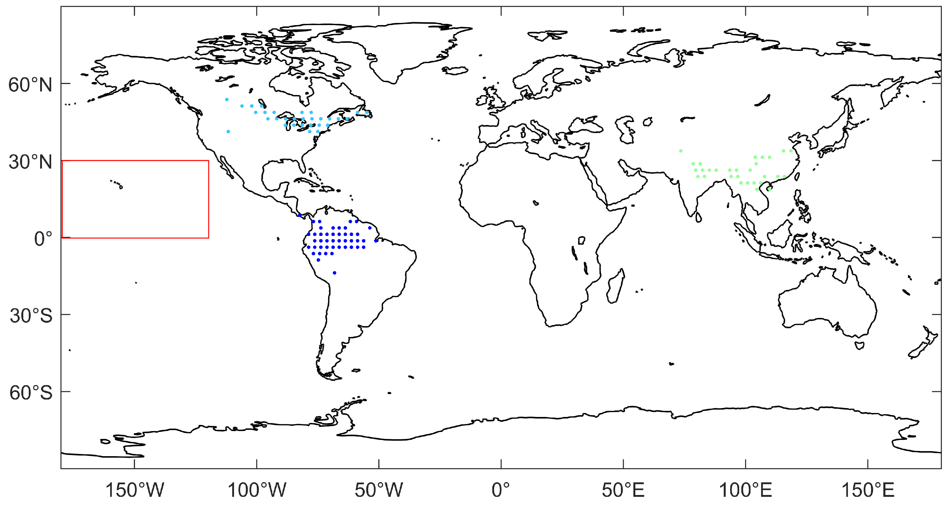
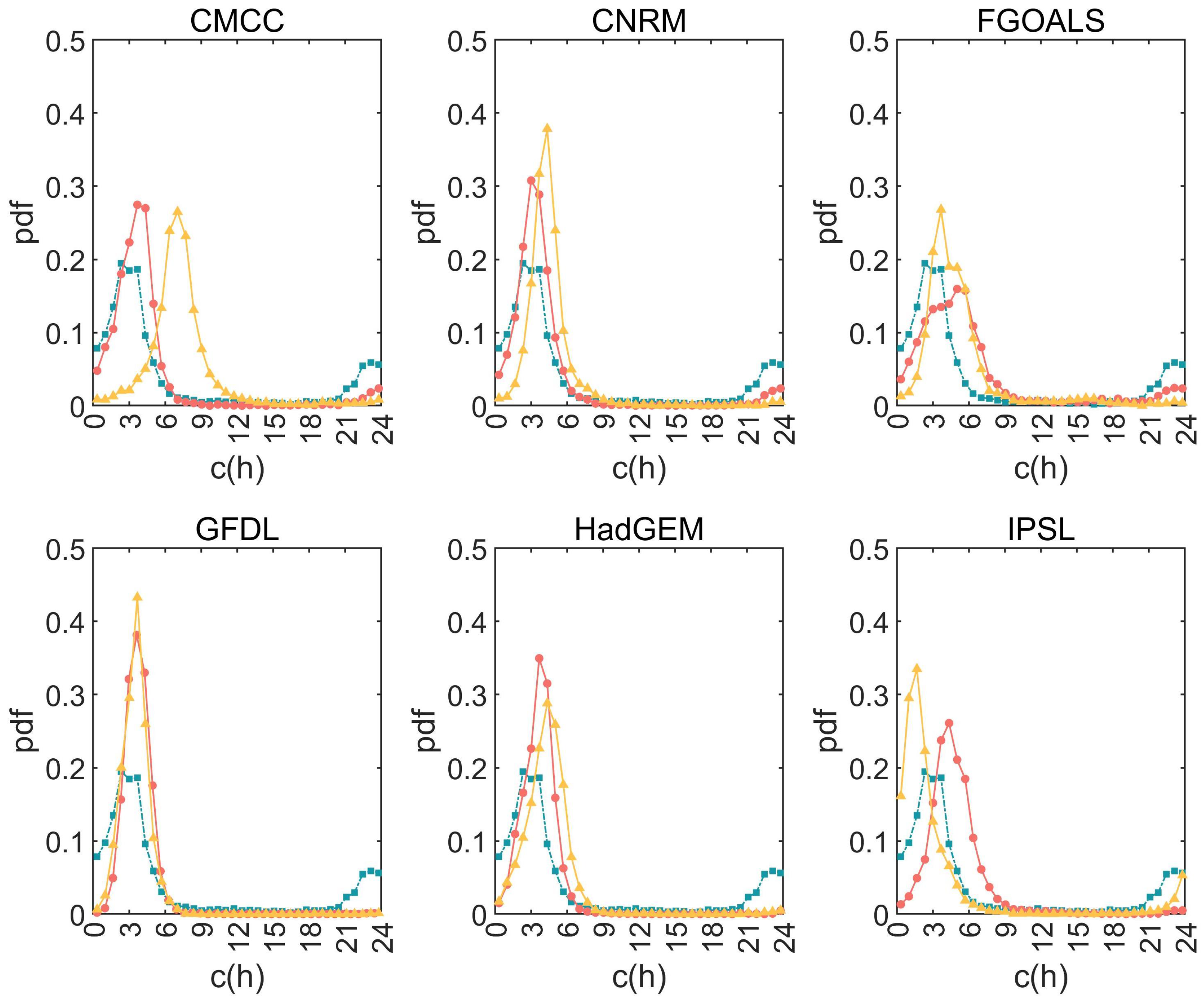
3.1. Regional Comparisons
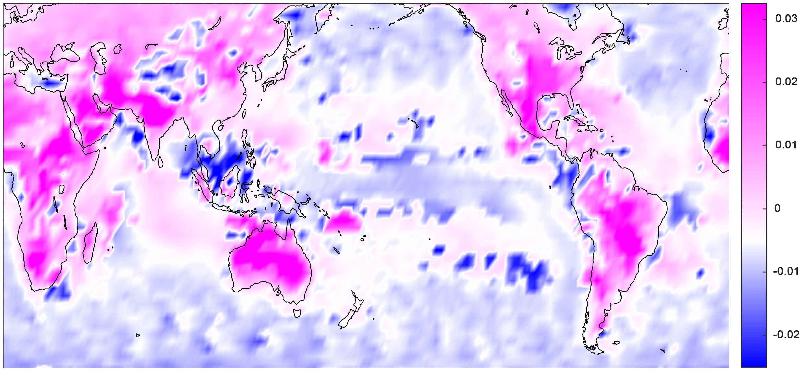
3.2. Global Distribution of DCC
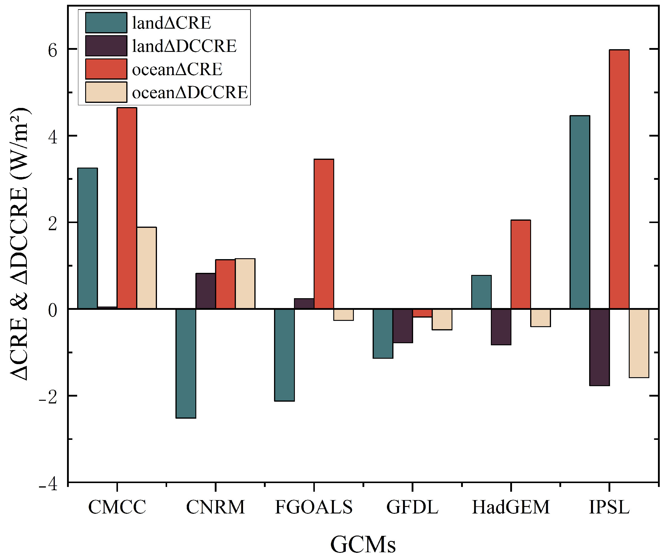
3.3. Radiative Effects of DCC Variations
4. Conclusions
Author Contributions
Funding
Institutional Review Board Statement
Informed Consent Statement
Data Availability Statement
Acknowledgments
Conflicts of Interest
Abbreviations
| DCC | Diurnal cloud cycle |
| CRE | Cloud radiative effects |
| DCCRE | Diurnal cloud cycle radiative effects |
| rlut | TOA outgoing longwave radiative flux (Wm−2) |
| rlutcs | TOA outgoing clear-sky longwave radiative flux (Wm−2) |
| rsut | TOA outgoing shortwave radiative flux (Wm−2) |
| rsutcs | TOA outgoing clear-sky shortwave radiative flux (Wm−2) |
References
- Norris, J.R.; Allen, R.J.; Evan, A.T.; Zelinka, M.D.; O’Dell, C.W.; Klein, S.A. Evidence for climate change in the satellite cloud record. Nature 2016, 536, 72–75. [Google Scholar] [CrossRef]
- Masson-Delmotte, V.; Zhai, P.; Pirani, A.; Connors, S.L.; Péan, C.; Berger, S.; Caud, N.; Chen, Y.; Goldfarb, L.; Gomis, M.; et al. Climate Change 2021: The Physical Science Basis. Contribution of Working Group I to the Sixth Assessment Report of the Intergovernmental Panel on Climate Change; Cambridge University Press: Cambridge, UK, 2021; Volume 2. [Google Scholar]
- Boucher, O.; Randall, D.; Artaxo, P.; Bretherton, C.; Feingold, G.; Forster, P.; Kerminen, V.M.; Kondo, Y.; Liao, H.; Lohmann, U.; et al. Clouds and aerosols. In Climate Change 2013: The Physical Science Basis. Contribution of Working Group I to the Fifth Assessment Report of the Intergovernmental Panel on Climate Change; Cambridge University Press: Cambridge, UK, 2013; pp. 571–657. [Google Scholar]
- Stephens, G.L. Cloud feedbacks in the climate system: A critical review. J. Clim. 2005, 18, 237–273. [Google Scholar] [CrossRef]
- Yin, J.; Porporato, A. Diurnal cloud cycle biases in climate models. Nat. Commun. 2017, 8, 2269. [Google Scholar] [CrossRef]
- Yin, J.; Porporato, A. Radiative effects of daily cycle of cloud frequency in past and future climates. Clim. Dyn. 2020, 54, 1625–1637. [Google Scholar] [CrossRef]
- Chen, G.; Wang, W.C.; Bao, Q.; Li, J. Evaluation of simulated cloud diurnal variation in CMIP6 climate models. J. Geophys. Res. Atmos. 2022, 127, e2021JD036422. [Google Scholar] [CrossRef]
- Wu, R.; Chen, G.; Luo, Z.J. Strong Coupling in Diurnal Variations of Clouds, Radiation, Winds, and Precipitation during the East Asian Summer Monsoon. J. Clim. 2023, 36, 1347–1368. [Google Scholar] [CrossRef]
- Emanuel, K.A. Atmospheric Convection; Oxford University Press on Demand: Oxford, UK, 1994. [Google Scholar]
- Zhang, Y.; Klein, S.A. Mechanisms affecting the transition from shallow to deep convection over land: Inferences from observations of the diurnal cycle collected at the ARM Southern Great Plains site. J. Atmos. Sci. 2010, 67, 2943–2959. [Google Scholar] [CrossRef]
- Yin, J.; Albertson, J.D.; Porporato, A. A probabilistic description of entrainment instability for cloud-topped boundary-layer models. Q. J. R. Meteorol. Soc. 2017, 143, 650–660. [Google Scholar] [CrossRef]
- Gentine, P.; Massmann, A.; Lintner, B.R.; Hamed Alemohammad, S.; Fu, R.; Green, J.K.; Kennedy, D.; Vilà-Guerau de Arellano, J. Land–atmosphere interactions in the tropics–a review. Hydrol. Earth Syst. Sci. 2019, 23, 4171–4197. [Google Scholar] [CrossRef]
- Wang, Z.; Ge, J.; Yan, J.; Li, W.; Yang, X.; Wang, M.; Hu, X. Interannual shift of tropical high cloud diurnal cycle under global warming. Clim. Dyn. 2022, 59, 3391–3400. [Google Scholar] [CrossRef]
- Mitchell, D.M.; Lo, Y.T.E.; Seviour, W.J.M.; Haimberger, L.; Polvani, L.M. The vertical profile of recent tropical temperature trends: Persistent model biases in the context of internal variability. Environ. Res. Lett. 2020, 15, 1040b4. [Google Scholar] [CrossRef]
- Ek, M.; Mahrt, L. Daytime evolution of relative humidity at the boundary layer top. Mon. Weather Rev. 1994, 122, 2709–2721. [Google Scholar] [CrossRef]
- Yin, J.; Albertson, J.D.; Rigby, J.R.; Porporato, A. Land and atmospheric controls on initiation and intensity of moist convection: CAPE dynamics and LCL crossings. Water Resour. Res. 2015, 51, 8476–8493. [Google Scholar] [CrossRef]
- Newman, M.; Alexander, M.A.; Ault, T.R.; Cobb, K.M.; Deser, C.; Di Lorenzo, E.; Mantua, N.J.; Miller, A.J.; Minobe, S.; Nakamura, H.; et al. The Pacific decadal oscillation, revisited. J. Clim. 2016, 29, 4399–4427. [Google Scholar] [CrossRef]
- Meehl, G.A.; Senior, C.A.; Eyring, V.; Flato, G.; Lamarque, J.F.; Stouffer, R.J.; Taylor, K.E.; Schlund, M. Context for interpreting equilibrium climate sensitivity and transient climate response from the CMIP6 Earth system models. Sci. Adv. 2020, 6, eaba1981. [Google Scholar] [CrossRef] [PubMed]
- Zelinka, M.D.; Myers, T.A.; McCoy, D.T.; Po-Chedley, S.; Caldwell, P.M.; Ceppi, P.; Klein, S.A.; Taylor, K.E. Causes of Higher Climate Sensitivity in CMIP6 Models. Geophys. Res. Lett. 2020, 47, e2019GL085782. [Google Scholar] [CrossRef]
- Schiro, K.A.; Su, H.; Ahmed, F.; Dai, N.; Singer, C.E.; Gentine, P.; Elsaesser, G.S.; Jiang, J.H.; Choi, Y.S.; David Neelin, J. Model spread in tropical low cloud feedback tied to overturning circulation response to warming. Nat. Commun. 2022, 13, 7119. [Google Scholar] [CrossRef] [PubMed]
- Eyring, V.; Bony, S.; Meehl, G.A.; Senior, C.A.; Stevens, B.; Stouffer, R.J.; Taylor, K.E. Overview of the Coupled Model Intercomparison Project Phase 6 (CMIP6) experimental design and organization. Geosci. Model Dev. 2016, 9, 1937–1958. [Google Scholar] [CrossRef]
- Soden, B.J.; Held, I.M.; Colman, R.; Shell, K.M.; Kiehl, J.T.; Shields, C.A. Quantifying climate feedbacks using radiative kernels. J. Clim. 2008, 21, 3504–3520. [Google Scholar] [CrossRef]
- Doelling, D.R.; Sun, M.; Nordeen, M.L.; Haney, C.O.; Keyes, D.F.; Mlynczak, P.E. Advances in geostationary-derived longwave fluxes for the CERES synoptic (SYN1deg) product. J. Atmos. Ocean. Technol. 2016, 33, 503–521. [Google Scholar] [CrossRef]
- Bergman, J.W.; Salby, M.L. The role of cloud diurnal variations in the time-mean energy budget. J. Clim. 1997, 10, 1114–1124. [Google Scholar] [CrossRef]
- Jammalamadaka, S.R.; Sengupta, A. Topics in Circular Statistics; World Scientific: Singapore, 2001; Volume 5. [Google Scholar]
- Jolliffe, I.T.; Cadima, J. Principal component analysis: A review and recent developments. Philos. Trans. R. Soc. A Math. Phys. Eng. Sci. 2016, 374, 20150202. [Google Scholar] [CrossRef]
- Beck, H.E.; Zimmermann, N.E.; McVicar, T.R.; Vergopolan, N.; Berg, A.; Wood, E.F. Present and future Köppen-Geiger climate classification maps at 1-km resolution. Sci. Data 2018, 5, 180214. [Google Scholar] [CrossRef] [PubMed]
- Webb, M.J.; Andrews, T.; Bodas-Salcedo, A.; Bony, S.; Bretherton, C.S.; Chadwick, R.; Chepfer, H.; Douville, H.; Good, P.; Kay, J.E.; et al. The cloud feedback model intercomparison project (CFMIP) contribution to CMIP6. Geosci. Model Dev. 2017, 10, 359–384. [Google Scholar] [CrossRef]
- Bony, S.; Webb, M.; Bretherton, C.; Klein, S.; Siebesma, P.; Tselioudis, G.; Zhang, M. CFMIP: Towards a better evaluation and understanding of clouds and cloud feedbacks in CMIP5 models. Clivar Exch. 2011, 56, 20–22. [Google Scholar]
- Schneider, T.; Bischoff, T.; Haug, G.H. Migrations and dynamics of the intertropical convergence zone. Nature 2014, 513, 45–53. [Google Scholar] [CrossRef] [PubMed]
- Nesbitt, S.W.; Zipser, E.J. The diurnal cycle of rainfall and convective intensity according to three years of TRMM measurements. J. Clim. 2003, 16, 1456–1475. [Google Scholar] [CrossRef]
- Lee, Y.C.; Wang, Y.C. Evaluating Diurnal Rainfall Signal Performance from CMIP5 to CMIP6. J. Clim. 2021, 34, 7607–7623. [Google Scholar] [CrossRef]
- Bai, L.; Chen, G.; Huang, L. Convection Initiation in Monsoon Coastal Areas (South China). Geophys. Res. Lett. 2020, 47. [Google Scholar] [CrossRef]
- Li, J.; Yu, R.; Zhou, T. Seasonal Variation of the Diurnal Cycle of Rainfall in Southern Contiguous China. J. Clim. 2008, 21, 6036–6043. [Google Scholar] [CrossRef]
- Li, X.; Lu, R.; Wang, X. Effect of Large-scale Circulation Anomalies on Summer Rainfall over the Yangtze River Basin: Tropical versus Extratropical. J. Clim. 2023, 36, 4571–4587. [Google Scholar] [CrossRef]
- Deser, C.; Wallace, J.M. Large-Scale Atmospheric Circulation Features of Warm and Cold Episodes in the Tropical Pacific. J. Clim. 1990, 3, 1254–1281. [Google Scholar] [CrossRef]
- Watters, D.; Battaglia, A.; Allan, R.P. The Diurnal Cycle of Precipitation according to Multiple Decades of Global Satellite Observations, Three CMIP6 Models, and the ECMWF Reanalysis. J. Clim. 2021, 34, 5063–5080. [Google Scholar] [CrossRef]
- Christopoulos, C.; Schneider, T. Assessing biases and climate implications of the diurnal precipitation cycle in climate models. Geophys. Res. Lett. 2021, 48, e2021GL093017. [Google Scholar] [CrossRef]
- Sun, Q.; Miao, C.; Duan, Q.; Ashouri, H.; Sorooshian, S.; Hsu, K.L. A review of global precipitation data sets: Data sources, estimation, and intercomparisons. Rev. Geophys. 2018, 56, 79–107. [Google Scholar] [CrossRef]
- Tang, S.; Gleckler, P.; Xie, S.; Lee, J.; Ahn, M.S.; Covey, C.; Zhang, C. Evaluating the diurnal and semidiurnal cycle of precipitation in CMIP6 models using satellite-and ground-based observations. J. Clim. 2021, 34, 3189–3210. [Google Scholar]
- Wild, M. The global energy balance as represented in CMIP6 climate models. Clim. Dyn. 2020, 55, 553–577. [Google Scholar] [CrossRef]
- Cherchi, A.; Fogli, P.G.; Lovato, T.; Peano, D.; Iovino, D.; Gualdi, S.; Masina, S.; Scoccimarro, E.; Materia, S.; Bellucci, A.; et al. Global mean climate and main patterns of variability in the CMCC-CM2 coupled model. J. Adv. Model. Earth Syst. 2019, 11, 185–209. [Google Scholar] [CrossRef]
- Park, S.; Bretherton, C.S. The University of Washington shallow convection and moist turbulence schemes and their impact on climate simulations with the Community Atmosphere Model. J. Clim. 2009, 22, 3449–3469. [Google Scholar] [CrossRef]
- Park, S.; Bretherton, C.S.; Rasch, P.J. Integrating cloud processes in the Community Atmosphere Model, version 5. J. Clim. 2014, 27, 6821–6856. [Google Scholar] [CrossRef]
- Iacono, M.J.; Delamere, J.S.; Mlawer, E.J.; Shephard, M.W.; Clough, S.A.; Collins, W.D. Radiative forcing by long-lived greenhouse gases: Calculations with the AER radiative transfer models. J. Geophys. Res. Atmos. 2008, 113. [Google Scholar] [CrossRef]
- Voldoire, A.; Saint-Martin, D.; Sénési, S.; Decharme, B.; Alias, A.; Chevallier, M.; Colin, J.; Guérémy, J.F.; Michou, M.; Moine, M.P.; et al. Evaluation of CMIP6 deck experiments with CNRM-CM6-1. J. Adv. Model. Earth Syst. 2019, 11, 2177–2213. [Google Scholar] [CrossRef]
- Guérémy, J. A continuous buoyancy based convection scheme: One-and three-dimensional validation. Tellus A Dyn. Meteorol. Oceanogr. 2011, 63, 687–706. [Google Scholar] [CrossRef]
- Piriou, J.M.; Redelsperger, J.L.; Geleyn, J.F.; Lafore, J.P.; Guichard, F. An approach for convective parameterization with memory: Separating microphysics and transport in grid-scale equations. J. Atmos. Sci. 2007, 64, 4127–4139. [Google Scholar] [CrossRef]
- Li, L.; Yu, Y.; Tang, Y.; Lin, P.; Xie, J.; Song, M.; Dong, L.; Zhou, T.; Liu, L.; Wang, L.; et al. The flexible global ocean-atmosphere-land system model grid-point version 3 (FGOALS-g3): Description and evaluation. J. Adv. Model. Earth Syst. 2020, 12, e2019MS002012. [Google Scholar] [CrossRef]
- Wu, X.; Deng, L.; Song, X.; Zhang, G.J. Coupling of convective momentum transport with convective heating in global climate simulations. J. Atmos. Sci. 2007, 64, 1334–1349. [Google Scholar] [CrossRef]
- Guo, Z.; Zhou, T. An improved diagnostic stratocumulus scheme based on estimated inversion strength and its performance in GAMIL2. Sci. China Earth Sci. 2014, 57, 2637–2649. [Google Scholar] [CrossRef]
- Shi, X.; Zhang, W.; Liu, J. Comparison of anthropogenic aerosol climate effects among three climate models with reduced complexity. Atmosphere 2019, 10, 456. [Google Scholar] [CrossRef]
- Stevens, B.; Fiedler, S.; Kinne, S.; Peters, K.; Rast, S.; Müsse, J.; Smith, S.J.; Mauritsen, T. MACv2-SP: A parameterization of anthropogenic aerosol optical properties and an associated Twomey effect for use in CMIP6. Geosci. Model Dev. 2017, 10, 433–452. [Google Scholar] [CrossRef]
- Sun, W.; Li, L.; Wang, B. Reducing the biases in shortwave cloud radiative forcing in tropical and subtropical regions from the perspective of boundary layer processes. Sci. China Earth Sci. 2016, 59, 1427–1439. [Google Scholar] [CrossRef]
- Zhao, M.; Golaz, J.C.; Held, I.; Guo, H.; Balaji, V.; Benson, R.; Chen, J.H.; Chen, X.; Donner, L.; Dunne, J.; et al. The GFDL global atmosphere and land model AM4. 0/LM4. 0: 1. Simulation characteristics with prescribed SSTs. J. Adv. Model. Earth Syst. 2018, 10, 691–734. [Google Scholar] [CrossRef]
- Zhao, M.; Golaz, J.C.; Held, I.; Guo, H.; Balaji, V.; Benson, R.; Chen, J.H.; Chen, X.; Donner, L.; Dunne, J.; et al. The GFDL global atmosphere and land model AM4. 0/LM4. 0: 2. Model description, sensitivity studies, and tuning strategies. J. Adv. Model. Earth Syst. 2018, 10, 735–769. [Google Scholar] [CrossRef]
- Williams, K.; Copsey, D.; Blockley, E.; Bodas-Salcedo, A.; Calvert, D.; Comer, R.; Davis, P.; Graham, T.; Hewitt, H.; Hill, R.; et al. The Met Office global coupled model 3.0 and 3.1 (GC3. 0 and GC3. 1) configurations. J. Adv. Model. Earth Syst. 2018, 10, 357–380. [Google Scholar] [CrossRef]
- Hourdin, F.; Jam, A.; Rio, C.; Couvreux, F.; Sandu, I.; Lefebvre, M.P.; Brient, F.; Idelkadi, A. Unified parameterization of convective boundary layer transport and clouds with the thermal plume model. J. Adv. Model. Earth Syst. 2019, 11, 2910–2933. [Google Scholar] [CrossRef]
- Rochetin, N.; Couvreux, F.; Grandpeix, J.Y.; Rio, C. Deep convection triggering by boundary layer thermals. Part I: LES analysis and stochastic triggering formulation. J. Atmos. Sci. 2014, 71, 496–514. [Google Scholar] [CrossRef]
- Rochetin, N.; Grandpeix, J.Y.; Rio, C.; Couvreux, F. Deep convection triggering by boundary layer thermals. Part II: Stochastic triggering parameterization for the LMDZ GCM. J. Atmos. Sci. 2014, 71, 515–538. [Google Scholar] [CrossRef]
 ), CMIP6 (
 ), and ISCCP (
 ).
), CMIP6 (), and ISCCP ().
).
), CMIP6 (), and ISCCP ().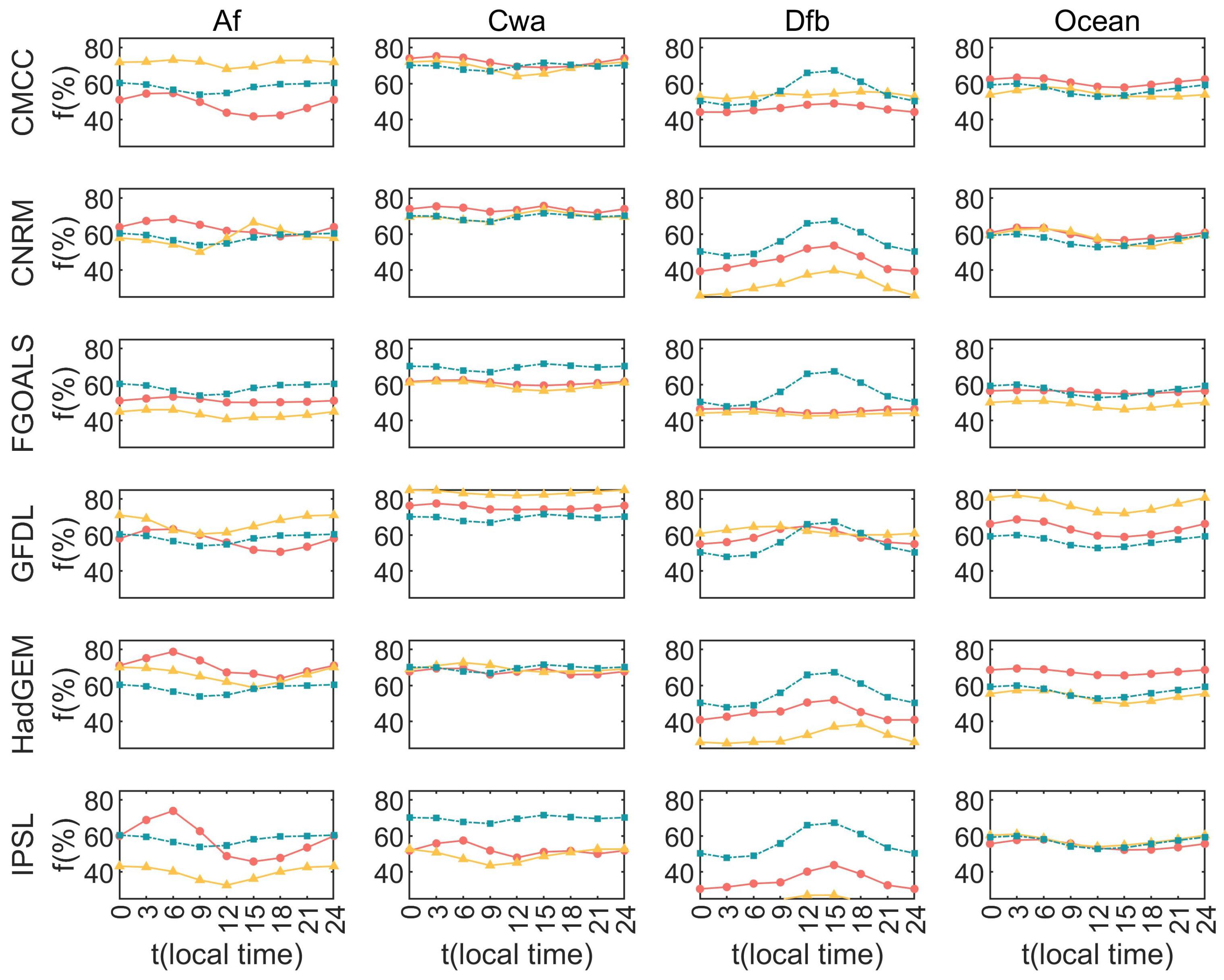
 ), CMIP6 (), and ISCCP ().
), CMIP6 (), and ISCCP ().
), CMIP6 (), and ISCCP ().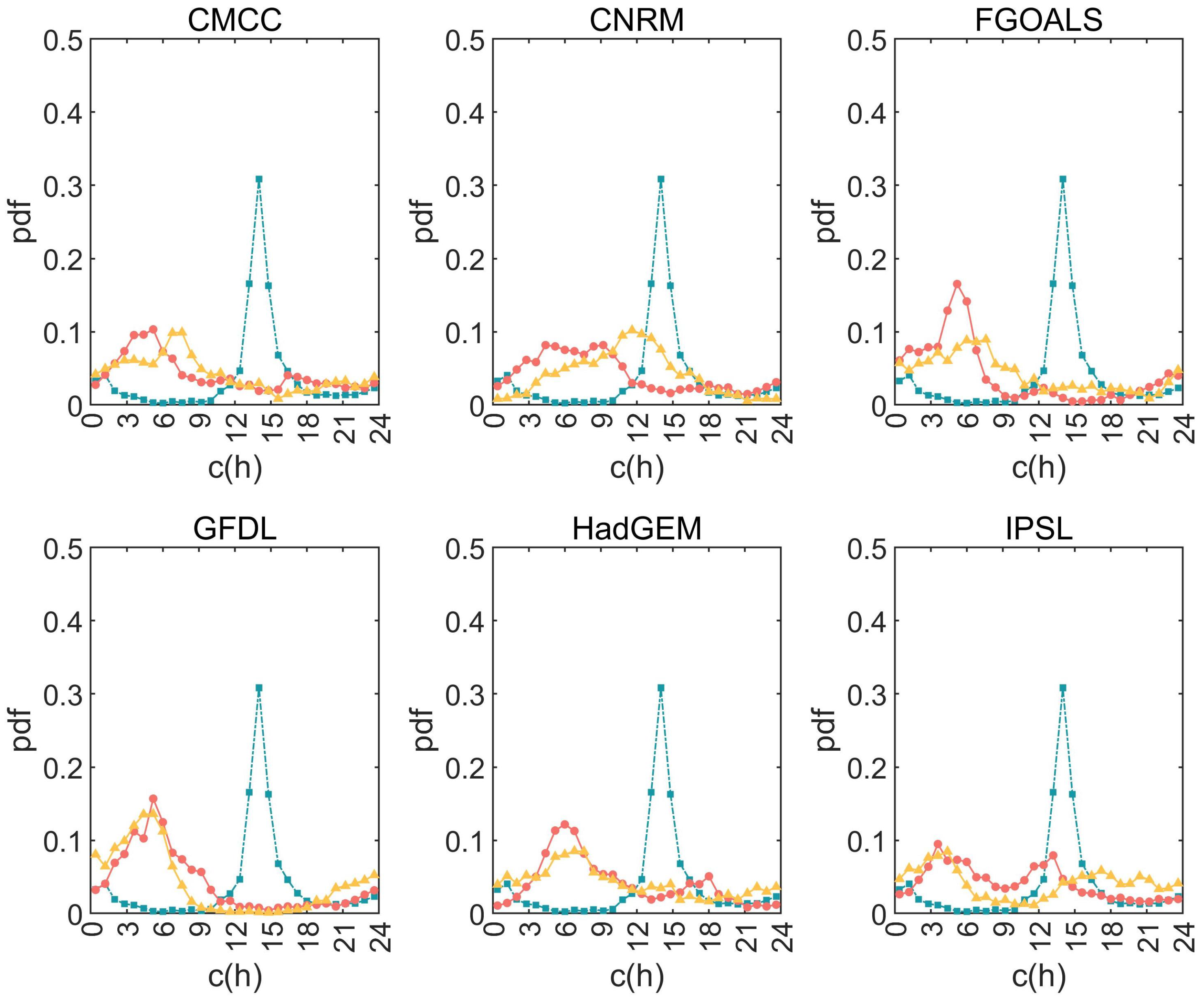


| Institute | Model Name | CMIP | Res. |
|---|---|---|---|
| CMCC | CMCC-CM | 5 | 1.33° × 0.75° |
| CMCC-CM2-SR5 | 6 | 1.25° × 0.94° | |
| CNRM-CERFACS | CNRM-CM5 | 5 | 1.41° × 1.41° |
| CNRM-CM6-1 | 6 | 1.41° × 1.41° | |
| LASG-CESS | FGOALS-g2 | 5 | 2.81° × 3.00° |
| CAS | FGOALS-g3 | 6 | 2.00° × 2.25° |
| NOAA-GFDL | GFDL-CM3 | 5 | 2.5° × 2.00° |
| GFDL-CM4 | 6 | 1.25° × 1.00° | |
| MOHC | HadGEM2-ES | 5 | 1.875° × 1.25° |
| HadGEM3-GC31-LL | 6 | 1.875° × 1.25° | |
| IPSL | IPSL-CM5A-MR | 5 | 2.5° × 1.26° |
| IPSL-CM6A-LR | 6 | 2.5° × 1.25° |
Disclaimer/Publisher’s Note: The statements, opinions and data contained in all publications are solely those of the individual author(s) and contributor(s) and not of MDPI and/or the editor(s). MDPI and/or the editor(s) disclaim responsibility for any injury to people or property resulting from any ideas, methods, instructions or products referred to in the content. |
© 2024 by the authors. Licensee MDPI, Basel, Switzerland. This article is an open access article distributed under the terms and conditions of the Creative Commons Attribution (CC BY) license (https://creativecommons.org/licenses/by/4.0/).
Share and Cite
Jiang, Z.; An, Y.; Yin, J. Comparison of Coupled Model Intercomparison Project Phases 5 and 6 in Simulating Diurnal Cloud Cycle. Atmosphere 2024, 15, 381. https://doi.org/10.3390/atmos15030381
Jiang Z, An Y, Yin J. Comparison of Coupled Model Intercomparison Project Phases 5 and 6 in Simulating Diurnal Cloud Cycle. Atmosphere. 2024; 15(3):381. https://doi.org/10.3390/atmos15030381
Chicago/Turabian StyleJiang, Zhiye, Yahan An, and Jun Yin. 2024. "Comparison of Coupled Model Intercomparison Project Phases 5 and 6 in Simulating Diurnal Cloud Cycle" Atmosphere 15, no. 3: 381. https://doi.org/10.3390/atmos15030381
APA StyleJiang, Z., An, Y., & Yin, J. (2024). Comparison of Coupled Model Intercomparison Project Phases 5 and 6 in Simulating Diurnal Cloud Cycle. Atmosphere, 15(3), 381. https://doi.org/10.3390/atmos15030381