Article

Influence of Various Urban Morphological Parameters on Urban Canopy Ventilation: A Parametric Numerical Study

1
School of Atmospheric Sciences, Sun Yat-sen University, and Southern Marine Science and Engineering Guangdong Laboratory (Zhuhai), Zhuhai 519082, China
2
Key Laboratory of Urban Meteorology, China Meteorological Administration, Beijing 100089, China
3
China Meteorological Administration Xiong’an Atmospheric Boundary Layer Key Laboratory, Xiong’an 071700, China
4
School of Civil Engineering, Chongqing University, Chongqing 400045, China
*
Author to whom correspondence should be addressed.
Atmosphere 2024, 15(3), 352; https://doi.org/10.3390/atmos15030352
Submission received: 29 December 2023 / Revised: 10 March 2024 / Accepted: 11 March 2024 / Published: 13 March 2024
(This article belongs to the Special Issue Urban Micro-Meteorological Researches)

Abstract

:
Numerical simulation is vital for evaluating urban ventilation. However, accurate urban-scale ventilation modeling requires extensive building surface simulation for computational demand. The distributed drag force approach simplifies the urban canopy by modeling buildings as a porous volume that accounts for momentum and turbulence. This method is a practical solution for simulating urban airflow. The drag force coefficient (Cd) is a crucial aerodynamic parameter in this approach. This study examines how Cd varies with urban design parameters such as plan area density (λp), average building height (H), frontal area density (λf), floor aspect ratio (AR), and sky view factor (SVF). Employing extensive numerical simulations conducted under neutral atmospheric conditions, we explore ranges of λp = 0.04–0.07 and λf = 0.1–1.2. The numerical model has been validated against existing wind tunnel data. The results show that Cd is insensitive to the model scale and background wind speed. We discover a nonlinear relationship between Cd and the parameters λp, λf, and SVF. For urban layouts with cubic-shaped buildings, Cd peaks at different λp within the range of 0.2~0.8. When λp and H are constant, Cd has a linear relationship with AR and λf. It is recommended to use λp, SVF, and AR as predictors for Cd across various urban configurations.

1. Introduction

Densely built-up cities suffer from problems such as the accumulation of pollutants from traffic [1], wind discomfort in the pedestrian zones [2], and haze–fog episodes [3,4]. Therefore, it is important to predict, evaluate, and optimize ventilation conditions within the urban canopy. Urban ventilation is a complex phenomenon influenced by the layout and density of buildings and has been the subject of extensive research at scales ranging from individual neighborhoods to entire cities, using experimental, numerical, and analytical methods [5,6,7].
At building and neighborhood scales, computational fluid dynamics (CFD) can predict detailed wind flow characteristics with highly realistic building shapes [8,9], with the stagnant zones and negative wake flow regions between buildings well resolved. However, the high computational cost of these detailed simulations limits their use at larger scales. To overcome this obstacle, some city-level numerical studies simplify an entire city into basic shapes [10,11], but this can compromise accuracy. A promising alternative that can reduce computational cost is to simplify building clusters as porous control volumes. This method is often referred to as the “macroscopic” method or “distributed drag force” method [11,12,13,14,15], where source terms are added to flow and turbulent models [12,13]. These methods can be divided into two types. One is inspired by the vegetation canopy models, where the drag force is determined by the drag force coefficient Cd and the frontal area density λf (hereafter referred to as the Cd·λf method). Cd can be calculated using the total force acting on the surface and the mean velocity in a control volume. Another method is based on the classical porous media approach, where the source terms consist of the Forchheimer and Darcy terms, which are determined by porosity (the total volume of air in the given volume) and permeability [16]. In both methods, the drag force coefficient Cd is a key parameter describing the influence of obstacles on the flow in the canopy.
Various urban morphological parameters are closely related to Cd, such as the plan area density (λp, the percentage of building floor area to the plan area), the frontal area density (λf, the percentage of the frontal area of buildings to the plan area) [17,18,19,20], the average height of the buildings [21,22,23,24], etc. Current knowledge of the relationships between urban morphology and Cd is primarily developed from idealized urban canopy models, in which buildings are simplified as arrays of cubes. These studies have revealed that how spatial parameters affect Cd varies with array configurations [25,26,27,28]. For instance, Kanda et al. [25] investigated cube arrays with a plan area density of 0–40% using large eddy simulation (LES) and found that Cd was sensitive to λp for staggered arrays but not for square arrays. Hagishima et al. [26] expanded on this by conducting wind tunnel experiments on 63 block arrays with different layouts, wind directions, block heights, and plan area densities. They found that Cd was more sensitive to λp and λf for staggered arrays than for square arrays. Ahmad Zaki et al. [27] also used wind tunnel tests to introduce variability in building orientation and height for building blocks and found that for arrays with a plan area density of 7.7~48.1%, vertical random arrays showed a consistent increase in Cd with λf. However, for horizontally random arrays, the estimated Cd peaked at a certain point. Li et al. [24] further investigated the effects of building shape on Cd peaked by wind tunnel experiments on non-uniform building arrays with different shapes (rectangular and H-shaped), wind directions, plan area densities, and frontal area indices. They found that Cd changed significantly when the building floor shape changed from a rectangle to an H shape.
Most of these studies have considered buildings as blocks with square footprints, and these studies have collectively revealed basic relationships between Cd and spatial parameters. For example, the relationship between Cd and λp or λf is not simply linear. Cd typically increases λp until reaching a plateau at about λp = 0.3 [26,28]. Santiago and Martilli [28] have developed a more complex empirical equation, which relates Cd to λp (i.e., Cd = 3.32 λp when λp ≤ 0.29; and Cd = 1.85 when λp > 0.29). This relationship has been used in later studies [29] to perform mesoscale simulations of local wind circulation. However, these correlations have been obtained from small samples, and the relationships between Cd and different spatial parameters (e.g., λp and λf) are often studied separately. Moreover, it is also necessary to extend the range of λp and λf values to cover real cities.
This study aims to investigate how the drag force coefficient Cd of idealized urban canopies behaves in a variety of morphological conditions. A parametric analysis is employed focusing on morphological parameters including SVF, λp, and λf. We conduct an extensive series of three-dimensional Reynolds-averaged Navier–Stokes (RANS) numerical simulations on both cubic and rectangular block arrays with λp = 0.04~0.7 and λf = 0.1~1.2. The findings have the potential to refine the application of the drag force approach in real-world wind environment assessments.

2. Methodology

2.1. RANS Canopy Model with Drag Force Approach

Both the Reynolds-averaged Navier–Stokes (RANS) model and large eddy simulations (LESs) are widely used in CFD simulation for urban micro-climate studies [30,31,32,33]. The LES model has pretty good precision in simulating and predicting turbulence [34,35,36]. However, enormous computational resources are required for the LES model. To save the computational resources, RANS simulation is employed in our study. The standard k-ε model is employed owing to its astonishing performance in predicting airflow [37,38,39]. In our previous work, we also evaluated the performance of three turbulence models (i.e., standard k-ε model, RNG k-ε model, and realizable k-ε model) compared to wind tunnel data [40]. The standard k-ε model has the best performance among the tested models, especially within the layer from the surface to the building rooftop (i.e., Height = 1H), where the drag force impacts crucially on the flow.
The urban context is characterized as a homogeneous control volume with regular building blocks and square floors (Figure 1). For this control volume, the drag force and mean flow parameters can be obtained from steady-state RANS simulation, where building surfaces are explicitly resolved in the mesh.
In this study, we conceptualize an idealized urban canopy as a series of regularly aligned rectangular blocks. As an example of a single control volume with four rectangular blocks (Figure 1a), Ap is the total floor area, Af is the frontal area of all buildings, H is the average height of the blocks, B is the width of block floor facing the wind, L is the length of block floor along the wind direction, and W is the street width. AB is the area of each floor, i.e., AB = B × L. The plan area density λp can be calculated using Equation (1):
λ p = A B / A p = B × L / ( B + W ) / ( L + W )
Frontal area density λf can be calculated with the following equation:
λ f = A f / A p = B × H / ( B + W ) / ( L + W )
Frontal area per unit volume Ai, i.e., projected area normal to the ith direction per unit volume of the control volume can be calculated with the following equation:
A i = A f / ( A p × H ) = B / ( B + W ) / ( L + W )
The porosity ϕ of the control volume can be calculated as follows:
ϕ = 1 λ p
The drag force acting on buildings (rectangular block arrays) can be represented by source terms added to the mean momentum equations, where the total drag force term Si in the ith direction can be calculated using Equation (5) [12,14]:
S i = ρ C d A i u i U S i = ρ C d A i u i U ,
where U is the velocity magnitude and ui is the velocity component in the ith direction. Cd is the drag force coefficient. Ai is not dimensionless, and its value changes with the scale of the model: the models with smaller dimensions have larger Ai. In contrast, for studies using the distributed drag force approach, Ai often refers to the total projected surface area of all buildings facing the wind within the control volume [41]. In this study, the definition of Ai follows the latter definition. The definitions of λf vary across studies with different grid sizes. For example, in [18,19], the total projected frontal areas of the first-row buildings within a 100 m by 100 m area have been considered as λf.
Equations (6) and (7) are listed as follows for further application of the drag force coefficient Cd if it is required. Sk and Sε are source terms added to RANS k-ε equations. They represent the production and destruction of turbulence resulting from building obstruction.
S k = ρ C d A f [ β p U 3 β d U k ]
S ε = ρ C d [ C ε 4 β p ε k U 3 C ε 5 β d U ε ]
Af is the total volumetric frontal area of all the blocks within the control volume. Βp is the fraction of mean airflow kinetic energy lost by drag that is converted into turbulent kinetic energy. Βd is the dimensionless coefficient for the short-circulating turbulence cascade [42]. Cε4 and Cε5 are dimensionless coefficients. In this model, the drag terms play a similar role to the Forchheimer–Darcy terms (see [16] for detailed information), which also represent the turbulent kinetic energy loss due to form drag. The coefficient group (βp, βd, Cε4, Cε5) for the sources in the urban canopy model is still a controversial topic in the published literature. Available values for the coefficient group can be as follows: (βp, βd, Cε4, Cε5) = [(1, 4, 1.5, 1.5), (1, 4, 1.5, 0.6), (1, 5.1, 0.9, 0.9)] [43] for the researchers who are interested in the four coefficients. However, we will not discuss these four coefficients in this paper since this work focuses on how to calculate Cd and how Cd varies with the influence of key factors.
In some drag force approach studies, Cd is obtained at different heights by dividing the whole control volume into various layers of thin slabs [28,44,45]. In this paper, Cd refers to the bulk drag coefficient of the control volume obtained with total drag force and mean flow velocity and can be calculated with Equation (8), where Fi is the total drag force exerted on the building surfaces in the ith direction, v ¯ is the average velocity magnitude of the bulk control volume on the ith direction, and Ai is the frontal area per unit volume of buildings projecting to the ith direction.
C d = F i 0.5 ρ v ¯ 2 A i C d = F i 0.5 ρ v ¯ 2 A i
The drag force coefficient Cd is traditionally defined in the literature, particularly in experimental studies, as the ratio of the total surface shear stress τ0 to the kinetic energy of the fluid, which is related to the free stream wind velocity Uref. This is represented mathematically as Cd = τ0/0.5ρ·Uref [7,26], where ρ is the fluid density. However, the specific definition of Cd can vary depending on the aims of each study. In our study, we aim to understand how Cd varies in a way that can be applied to the drag force approach in macroscopic CFD simulations; the mean streamwise velocity is therefore used to calculate Cd.

2.2. Idealized Building Array Configurations

We conduct RANS simulations using the standard k-ε model to explore how urban canopy layout affects the drag force coefficient Cd. Two sets of spatial configurations have been investigated and the details are listed in Table 1 and Table 2. The geometric dimensions follow the illustrations in Figure 1.
The spatial configurations in Table 1 focus on the impact of plan area density λp, frontal area density λf, and sky view factor SVF on Cd. The building floor is considered to be square (B = L). The average building height (H) is in the range of 5–125 m to ensure that λf is in the range of 0.05–1.21. The street width is assumed to be fixed at 20 m or 30 m. The largest λp is limited to no more than 0.7, allowing for a minimum green coverage ratio (GCR) of 30%.
The second group In Table 2 focuses on the response of Cd to changing floor aspect ratio AR = B/L. This is necessary because real urban environments often feature buildings with rectangular floors. In this case, λf can be changed due to the stretch of the projected frontal plane in both the vertical and the horizontal direction. To reduce sample size and simulation time, 7 combinations of λp and building heights are designed.

2.3. Numerical Settings

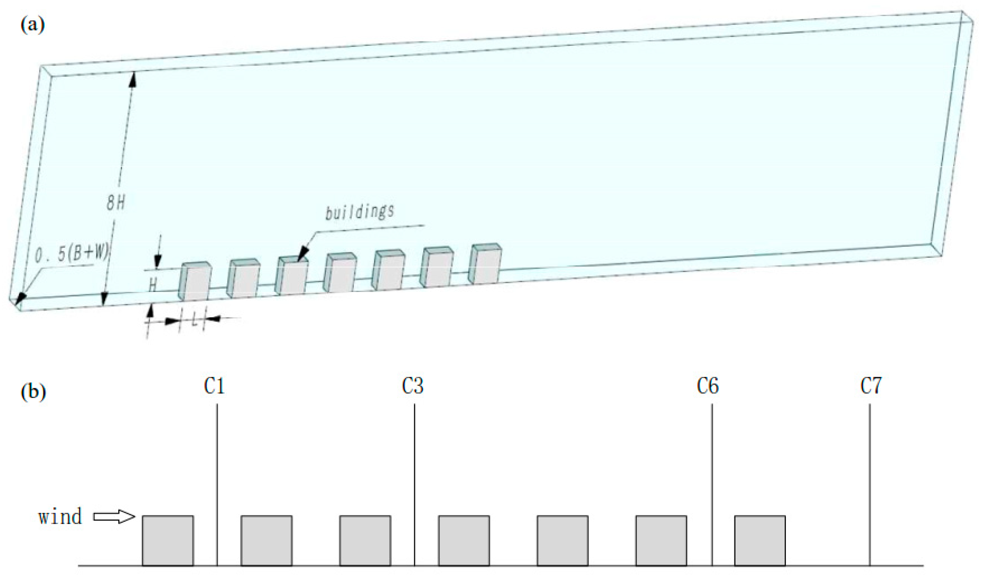
For each RANS simulation, a symmetric model is developed with several rows of building blocks repeated along with the flow direction, as shown in Figure 2a. The number of building rows is set to 14 to ensure a fully developed flow. However, in the validation study described in the following section, the number of rows is set to 7, being consistent with the wind tunnel study [46].
The numerical calculations are performed in Ansys Fluent. The boundary condition of the streamwise velocity for the domain inlet is provided by Equations (9)–(11) [46], where is 0.09, UH is 3.0 m/s, u = 0.24 m/s, kv is von Karman’s constant, and the value is 0.41 in this work.
U ( z ) = U H ( z / H ) 0.16
k ( z ) = u 2 / C μ
ε ( z ) = C μ 3 / 4 k ( z ) 3 / 2 / k v z
Standard wall functions are used for the ground, building walls, and roofs. Zero-gradient boundary conditions are used at the domain outlet and the domain top. The simulations were carried out using the pressure-based model. A second-order upwind discretization scheme was used to solve the momentum and turbulence equations. The PRESTO scheme was used for the pressure correction equation, and the SIMPLE algorithm was used for the pressure–velocity coupling. The convergence criteria for the scaled residuals were set as 10−4 for continuity, momentum, and turbulent equations. The geometry of the computational domain is extended to 8H in height, 8H in the windward direction, and 20H in the leeward direction.

2.4. Validation Study

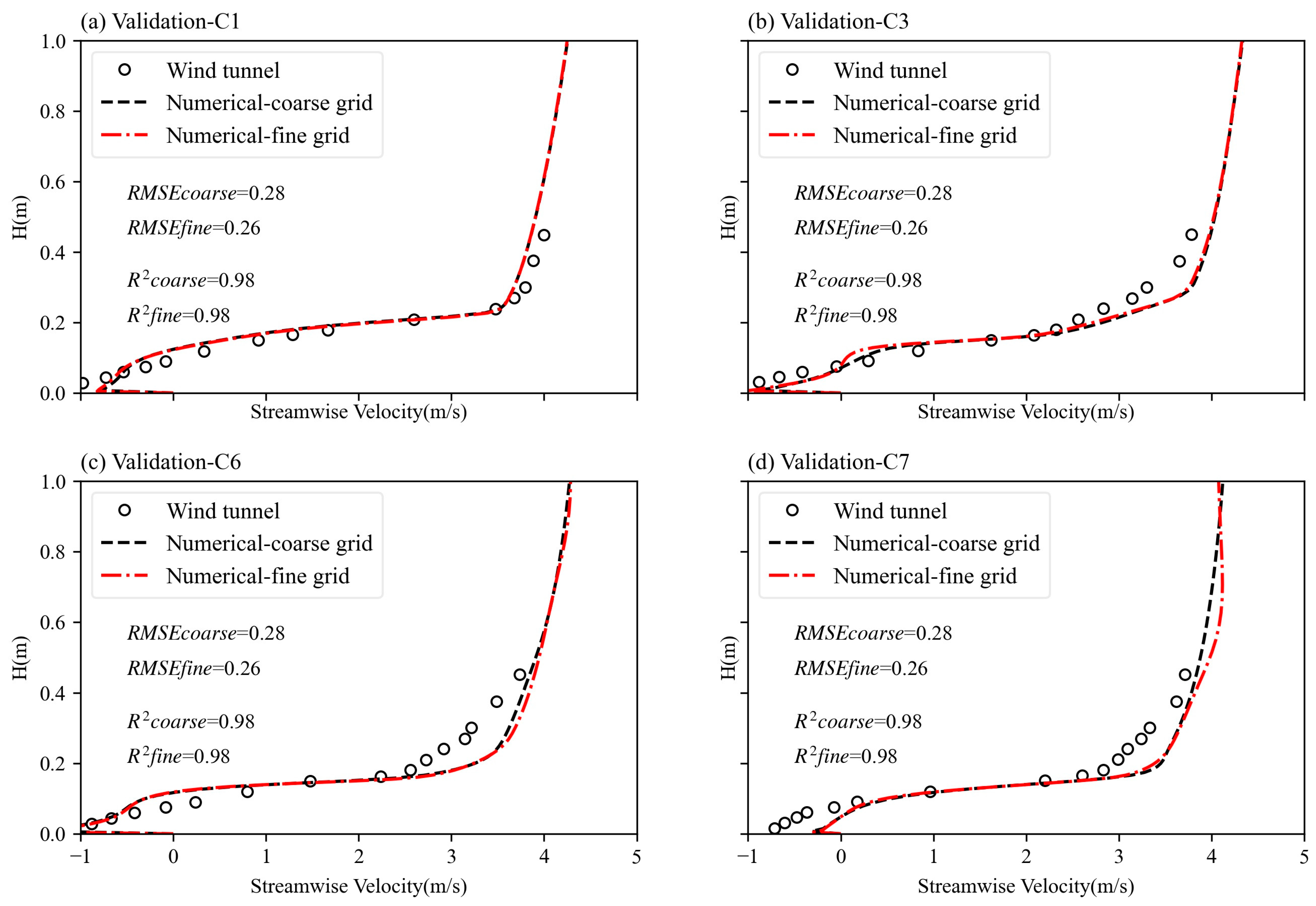
The validation model geometry (Figure 2a) follows the wind tunnel experiment by Lien et al. [46] with λp = 0.25. There are 7 rows of buildings, and the dimension of each cubic block is H = W = B = 0.15 m. The computational domain is 8H high in the vertical direction (z), 6.6H long in the streamwise direction (x), and 1H wide in the lateral direction (y) in the 3D model. The vertical profiles of streamwise velocity obtained from numerical simulations at the midpoints of 4 canyons (Figure 2b) on the leeward side of the 1st, 3rd, 6th, and 7th obstacles are compared to wind tunnel experiment results. The computation employs a structured grid, and to test the sensitivity of the numerical results to mesh size, we have compared 2 mesh sizes: a fine grid contains 962,444 cells (total grid numbers in x-, y-, and z-directions are 449, 28, and 81, respectively), while a coarse grid contains 684,860 cells (total grid numbers in x-, y-, and z-directions are 446, 22, and 73, respectively).
Figure 3 illustrates that the differences in results from the fine and coarse grid simulations are minimal, particularly within the canopy area. Important statistics for the simulation results of coarse and fine grids are also summarized in Figure 3, including the root mean square error (RMSE) and correlation coefficient (R2). The definitions of RMSE and R2 are shown as Equations (12) and (13), where n is the number of data points; ei = SiOi; and Si and Oi are simulated and observed values. The results show that the streamwise velocity (U) is nearly consistent across both grid sizes, indicating low grid sensitivity for the two sets of grids tested. However, some discrepancies occur in the wake region (C7) and just above the roof level. Despite these minor variations, the model well estimates velocities below the rooftop and is suitable for our parametric study.
R M S E = n 1 i = 1 n e i 2 0.5
R 2 = i = 1 n O i S i i = 1 n O i i = 1 n S i n i = 1 n O i 2 i = 1 n O i 2 n i = 1 n S i 2 i = 1 n S i 2 n 2

2.5. Effect of Model Scale and Background Wind Condition

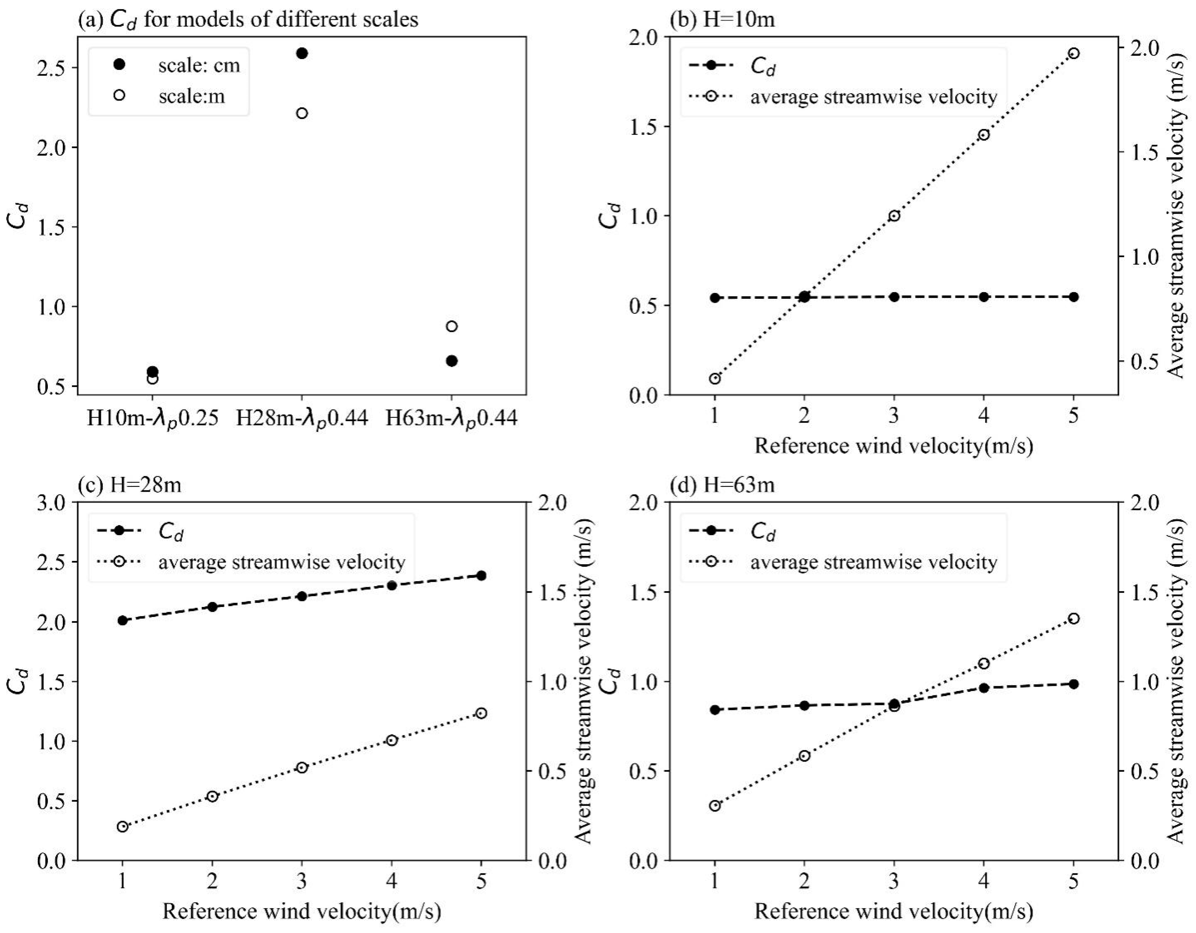
Understanding how the drag coefficient (Cd) varies with the model scale is the precondition of utilizing the drag force approach in wind assessment. Existing parameterization studies on Cd for building arrays tend to use reduced scale models in scales of centimeters and millimeters in wind tunnel and numerical studies. This study examines Cd across different scales (centimeters, decimeters, and meters) for three urban canopy types: low-rise low-density (H = 10 m, λp = 0.25), mid-rise high-density (H = 28 m, λp = 0.44), and high-rise high-density (H = 63 m, λp = 0.44). Figure 4a shows the Cd values for these scenarios, demonstrating that the scale of the model does not significantly affect Cd when morphological parameters are constant. This finding suggests that models with different reduced scales or full scales can use the same Cd value without introducing substantial errors. Subsequent sections of this paper will discuss parametric analyses conducted using full-scale numerical models.
The drag force coefficient Cd has also been compared across varying background wind speeds (1–5 m/s at 15 m height), as depicted in Figure 4b–d. The results show that the changes in Cd across different background wind speeds are small for cases with H = 10 m, λp = 0.25 and H = 63 m, λp = 0.44. For the mid-rise, high-density case (H = 28 m, λp = 0.44), where the value of Cd is comparably higher than the other two cases, there is a marginal increase in Cd with higher wind velocities, though the overall variation remains below 0.3. Therefore, we assume that Cd is insensitive to background wind velocity magnitude, and the values of Cd can thus be conveniently applied in practical wind assessment. On the other hand, though with the same λp, the value of Cd for the mid-rise canopy (H = 28 m, λp = 0.44) is almost double that of the high-rise canopy (H = 63 m, λp = 0.44), indicating that the momentum loss of wind speed per unit volume of the mid-rise dense canopy is larger. This contradicts the intuition that a high-rise cluster would result in greater momentum loss of wind.

3. Results and Discussion

3.1. Influence of Urban Morphology on Urban Ventilation in Rectangular Building Blocks

3.1.1. Influence of Urban Morphology on Surface Drag Force and Streamwise Velocity

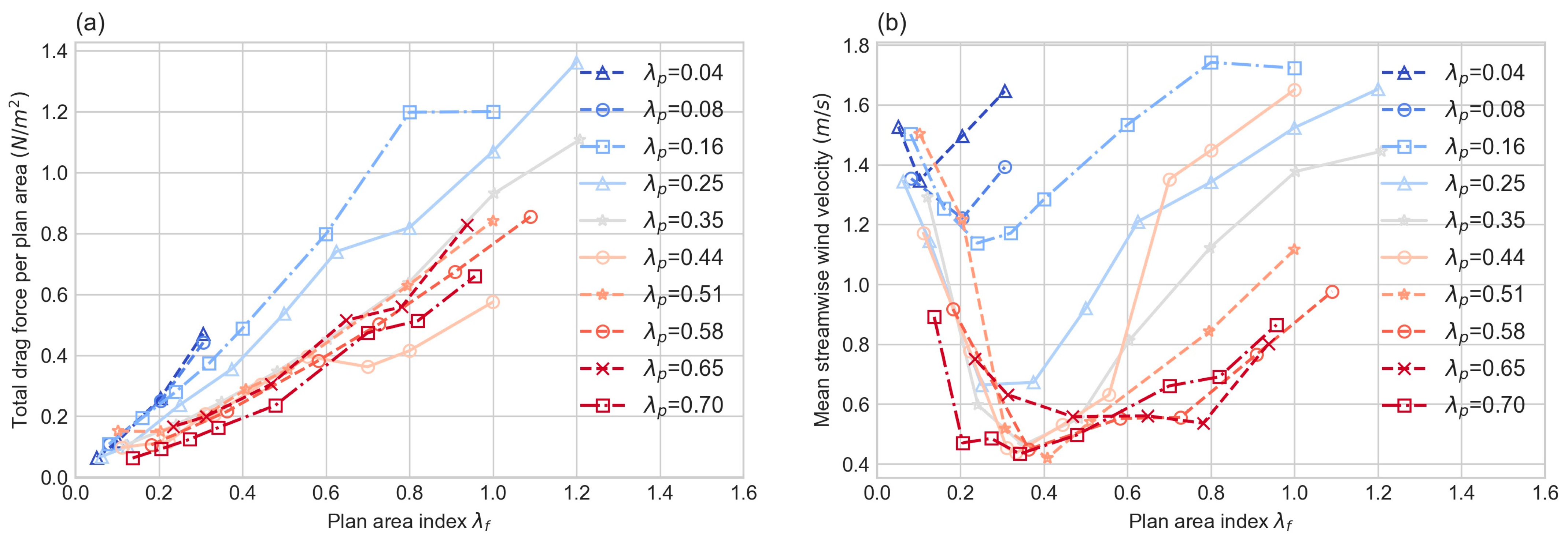
The total drag force in the control volume is directly related to the drag force coefficient Cd, a key non-dimensional parameter that influences the total surface shear stress and reference flow speed in the urban canopy, as described in the previous section. Figure 5a shows a positive linear relationship between the total drag per unit plan area and the frontal area density (λf), with a consistent rate of increase across different plan area densities (λp). This is in line with previous studies that reported an increase in Cd with the increase in λf [24,26]. However, it may appear counterintuitive that canopies with λp ≤ 0.35 experience a higher total drag per unit plan area than those with increased λp.
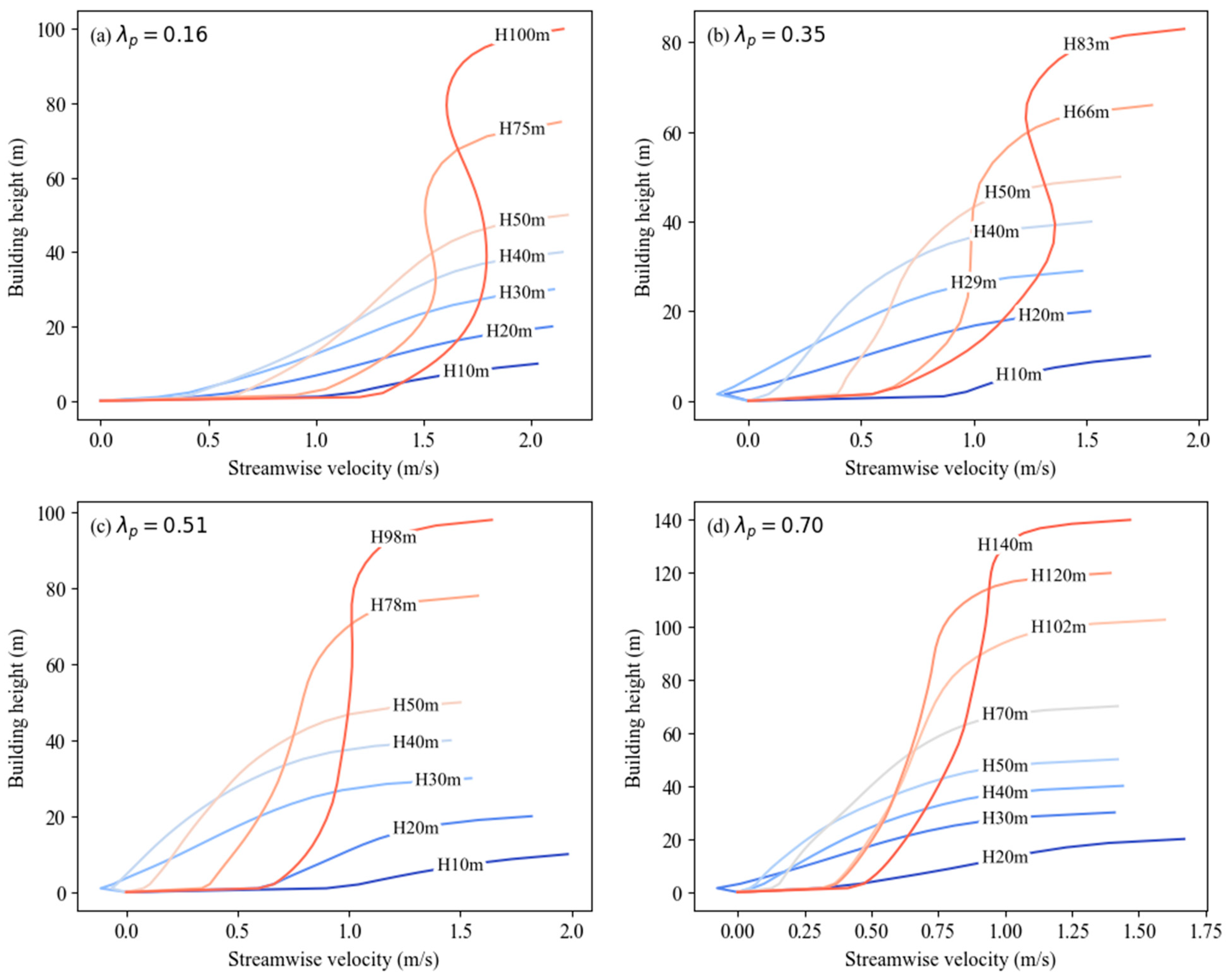
For the mean streamwise wind velocity, Figure 5b depicts its variation with λf and λp. The results reveal a V-shaped curve for the relationship between streamwise wind velocity and λf. The lowest streamwise wind velocity appears at an approximate λf of 0.3–0.4, being consistent across all the examined λp ranges. Furthermore, Figure 6 shows the spatial mean of the intra-canopy streamwise velocity (denoted as <uz>) at different heights for different λp and building heights. The <uz> at each height is obtained by averaging streamwise velocity at all the air cells in the control volume at the same height. The <uz> value consistently rises with height until it reaches a threshold for most canopies. However, <uz> in some canopies with higher heights (H = 75 m, 83 m, 100 m) and smaller λp (λp = 0.16, 0.35) has a distinctive S-shaped curve, which has two inflection points.
The above results suggest that the total drag force per unit area is more sensitive to λf than to λp. Though the drag force per unit area linearly increases with λf for any given λp, this does not imply a direct negative impact on ventilation performance. From the point of view of the city scale, the intra-canopy wind velocity directly reflects the average ventilation performance of one district, while the total drag force denotes the momentum loss of approaching wind at this control volume and directly affects its leeward control volume. Therefore, a medium λf (i.e., λf = 0.4 in our study) results in lower drag force, yet it can also lead to reduced wind velocity and poorer ventilation compared to a higher λf. Conversely, a high λf could cause greater momentum loss and subsequently degrade ventilation in downwind areas. It is the combined effect of both the drag force and the wind velocity in all control volumes of an urban canopy that controls the overall ventilation performance. In other words, the drag force coefficient Cd that developed from both drag force and intra-canopy velocity can be a better choice to denote ventilation performance.

3.1.2. Influence of Urban Morphology on Drag Force Coefficient Cd

With the first set in Table 1, we begin our analysis by considering a widely used assumption in similar studies: λp = λf and B = L = H, i.e., where the building block is cubic with equal dimensions for breadth (B), length (L), and height (H) and where the plan area index (λp) equals the frontal area density (λf) [7,28].
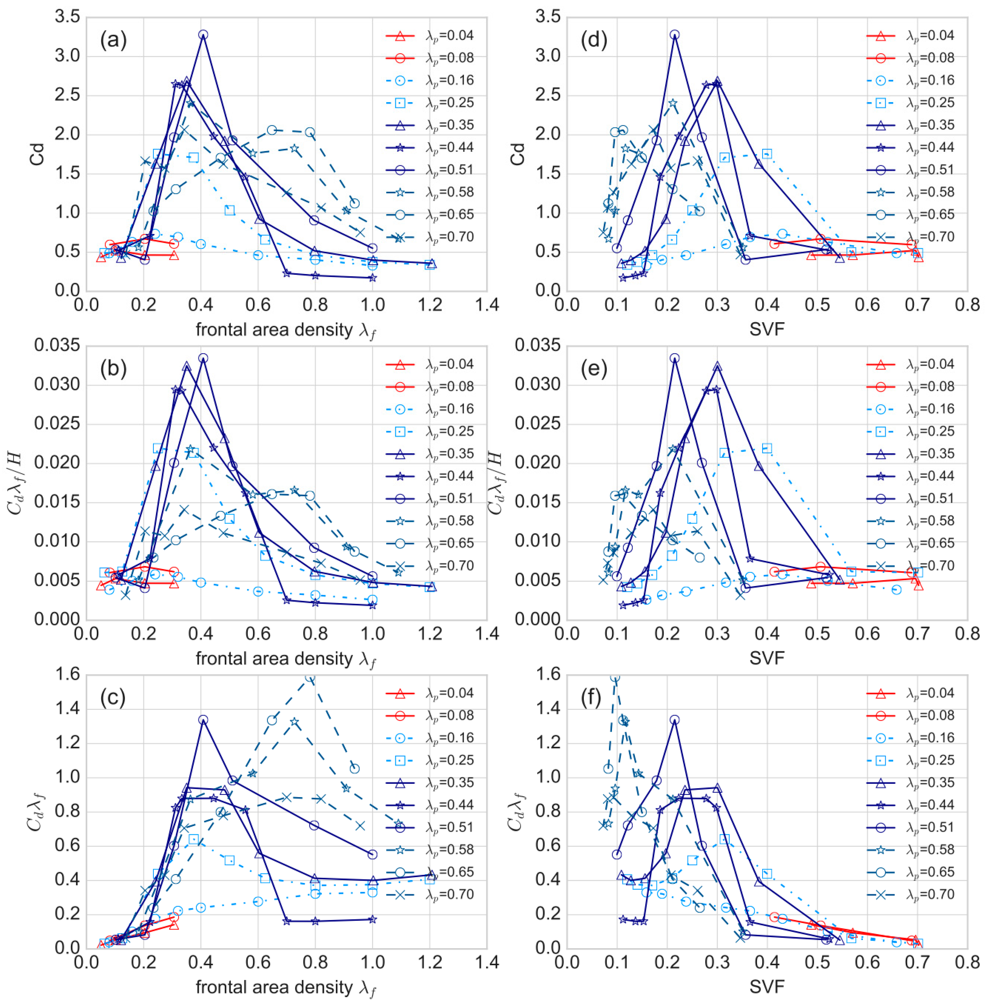
Figure 7a illustrates how the drag coefficient Cd is influenced by λp, λf, and SVF. Cd initially increases with λp before reaching a peak at approximately λp = 0.35, then undergoes a gradual decline, except when λp = 0.65. Notably, the decrease in Cd is more gradual compared to its increase. For a small λp (λp = 0.16), changes in Cd are minimal. However, for higher λp, the obstacles within the control volume increase with the increasing λp, and the momentum loss of wind increases. Owing to the wake interference flow or skimming flow regime, the obstruction of downstream buildings is weakened because of sheltering. This suggests a transition in flow characteristics within the canopy—from isolated flow with lower λp to wake interference or skimming flow with higher λp, where downstream building obstruction is reduced due to sheltering effects [47,48]. Our findings are closely aligned with those of Santiago et al. [28], who performed a parametric analysis on the variation in Cd using a uniform staggered array of cubes (where λp = λf) and derived an empirical equation (Equation (14)). The trend of Cd for λf values below 0.44 reported by Santiago et al. [28] is similar to our results. However, an intriguing behavior is noted where Cd noticeably decreases once λf surpasses 0.44.
C d = 3.32 λ p         λ p     0.29 1.85                 λ p > 0.29
Figure 7b shows the variation in Cd·λf/H with λf; the trend is similar to that of Cd. The maximum value of Cd·λf/H appears at approximately λf = 0.25–0.4. Similar to Cd, the physical meaning of Cd·λf/H is also clear: it represents the obstruction per unit volume of the urban canopy that induces momentum loss in the approaching wind. Cd·λf (Figure 7c) represents the obstruction per unit plan area of the urban canopy acting on the approaching wind, and it increases monotonously with the increase in λp. The trend is different from what is revealed for Cd and Cd·λf /H. For lower λp (0–0.51), Cd·λf peaks at where λf is around 0.35, while for higher λp (0.58–0.7), Cd·λf peaks at where λf is around 0.8.
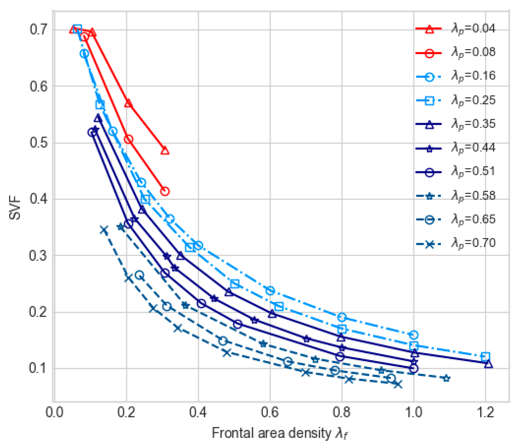
The results show that the effect of SVF on parameters Cd, Cd·λf/H, and Cd·λ (Figure 7d–f) shares both similarities and differences with the effect of λf. Across all cases in this study, we found that Cd is more likely to reach higher values when SVF is between 0.2 and 0.3, not at its lowest when the building clusters show the strongest sheltering effect. This observation diverges from the intuitive expectation that the maximum drag coefficient would coincide with the minimum openness. Particularly, in a densely populated urban area with λp of over 0.65, the peak value of Cd and Cd·λf/H is observed when SVF is approximately 0.1. Moreover, the relationship between SVF and Cd across varying λp values demonstrates a non-linear pattern: as SVF increases, Cd initially rises and then decreases. This trend suggests an SVF range where the drag coefficient is maximized, beyond which further increases in SVF lead to reductions in Cd. Furthermore, the underlying dynamics between SVF and λf (Figure 8) can help to understand this relationship. A relatively regular pattern is observed where an increase in λf leads to a decrease in SVF. This inverse relationship between SVF and λf makes the effect of SVF on parameters Cd, Cd·λf/H, and Cd·λ simpler to explain: in general, the smaller the SVF, the larger the parameters related to resistance.
The choice between using Cd·λf/H or Cd·λf as the indicator to describe the impact of turbulence on urban wind optimization depends on the optimization methodology employed. For example, for a GIS-based least-cost-path method (similar to that in [49]) that divides the city into a grid of patches, Cd·λf could be a more acceptable indicator since it directly implies the total momentum loss of wind on each grid. If only the lower level of the canopy (below the roof of mid-rise building clusters) is the optimized target, Cd·λf/H could also be a favorable indicator. Though current evidence is still insufficient to determine which one of the two indicators is superior, both of them are promising alternatives for the commonly used parameter λf.
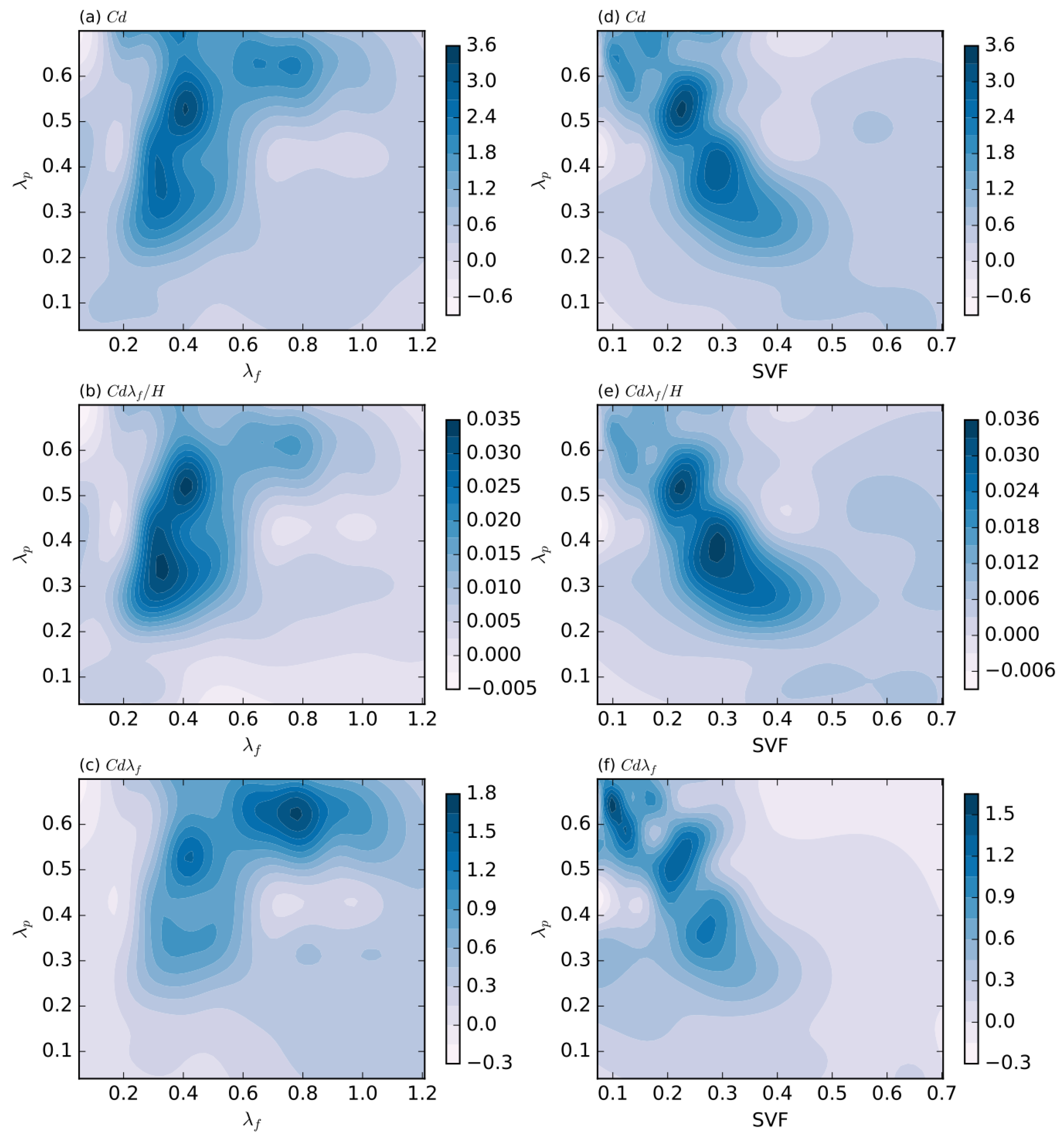
Figure 9a–c illustrate the interpolation results of Cd, Cd·λf/H, and Cd·λf with 2D contour graphs to further reveal the response of these three indicators under the combined effect of λp and λf. It can be seen that a local maximum of Cd and Cd·λf/H appears near (λp, λf) = (0.3~0.5, 0.4). A local maximum of Cd·λf appears near (λp, λf) = (0.6, 0.4~0.8). The trend of Cd in our results is almost identical to that of Santiago et al. [28] when λp is smaller than 0.44. Interestingly, Cd obviously decreases when λp exceeds 0.44. Urban buildings are influenced by their nearest surroundings, but lacking a detailed representation of the area is a huge challenge for accurate ventilation predictions. Figure 9d–f demonstrates how the combination of λp and SVF influences these resistance-related parameters (Cd, Cd·λf/H, and Cd·λf) through interpolation results. Unlike the effect of λf, these resistance parameters show an overall decreasing trend with the increase in SVF. The contour plots of Cd in Figure 9 could be used in macroscopic or drag force approach-based numerical simulations that can reduce mesh number and simplify the physical model (refer to [11,15]).

3.2. Effect of Building Floor AR (Aspect Ratio) on Drag Force Coefficient Cd

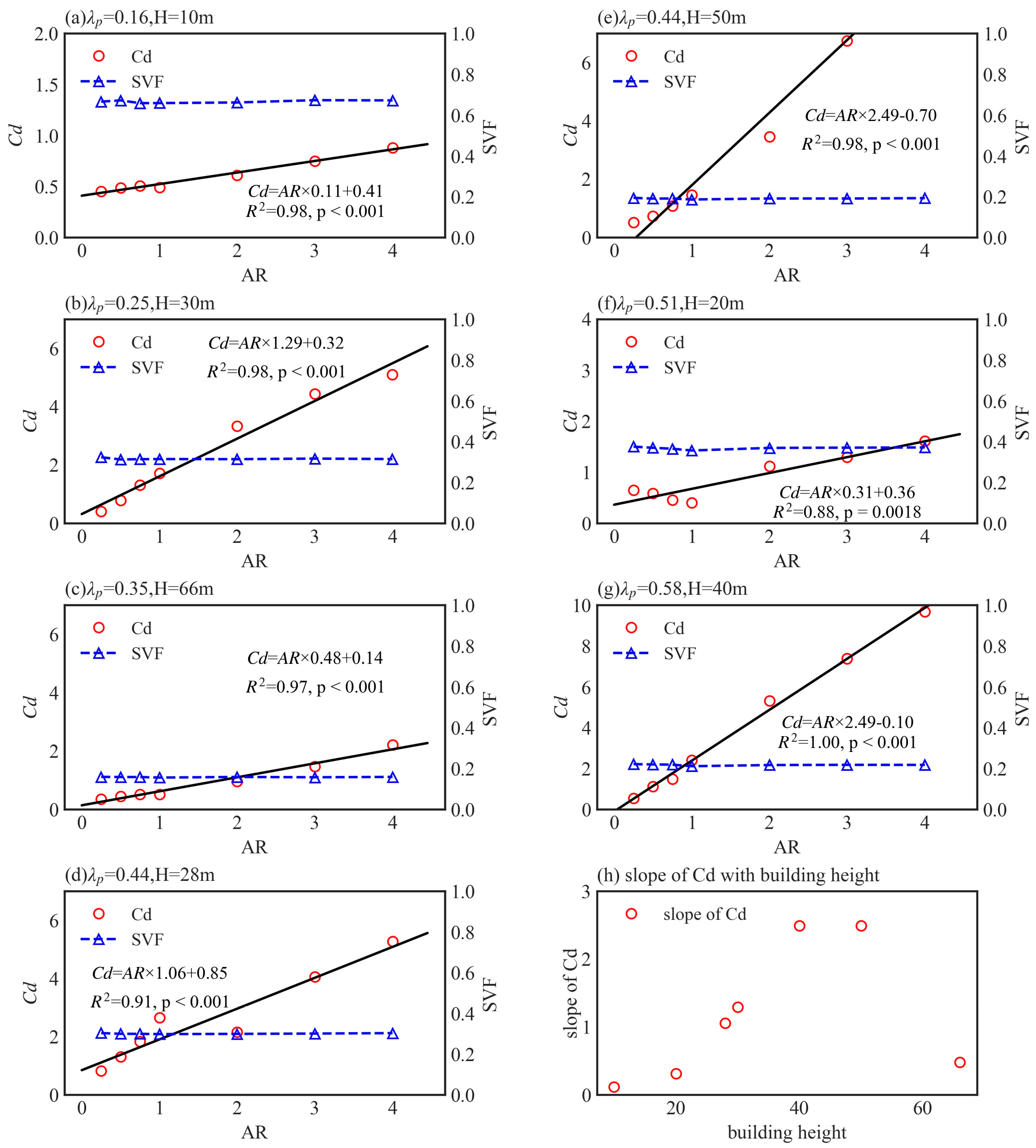
Previous sections focused on scenarios when λf = λp, where λf increases with rising building height. However, in real urban areas, λf also changes with the aspect ratio (AR) of the building floor. This section investigates the variation in Cd with changing building floor AR. This group of cases is designed with fixed variables (i.e., canopy height H, building plan area density λp, and street width W) listed in Table 2. Figure 10 illustrates that Cd increases linearly with AR, and the slope of Cd becomes the largest in canopies with larger λp and larger H (i.e., λp = 0.44, H = 50 m; and λp = 0.58, H = 40 m).
These results suggest that the aspect ratio of the building floor is also a significant factor that affects Cd. Despite having less research interests in GIS-aided urban ventilation studies compared to λp and λf, the significance of building floor AR requires more attention.
λf may increase due to taller buildings or larger building floor AR in urban planning. For a fixed H/W, a linear increase in Cd with rising λf is observed when it is related to floor length. However, Cd initially increases and then decreases with increasing λf for taller buildings. Therefore, considering the building floor AR reveals that neither λf nor λp can fully capture the variations in Cd in isolation. As shown in Figure 10, the sky view factor SVF changes little with building floor AR but is influenced by λp and H/W distinctly. This recommends a two-step approach to estimating Cd, starting with λp and SVF for a rough estimate, then refining it with the floor AR for better precision. Based on the above analysis, it is highly recommended to use three parameters (i.e., λp, SVF, and floor AR) to estimate the drag force coefficient Cd for a given urban area. In addition, using λp, λf, and floor AR for Cd estimation is reasonable too. Although the logic between λf and Cd still needs comprehensive exploration, it is possible to develop relationships and is easier to obtain frontal area density for practical design activities with the GIS technique.
The question of whether taking urban surfaces as regular geometry is still open, and the effect of spatial inhomogeneity can be a future research direction. A limitation of this macroscopic model is the reliance on a substantial number of obstacles within the representative element volume for accurate predictions. The model precision is reduced in areas with few obstacles or where the airflow is not fully developed.

3.3. Limitations and Future Work

In this study, we focused on evaluating the impact of various urban design parameters, such as plan area density (λp), average building height (H), frontal area density (λf), floor aspect ratio (AR), and sky view factor (SVF) on the drag force coefficient (Cd) using numerical simulations under neutral atmospheric conditions. Our research aimed to provide insights into how these parameters influence urban ventilation, leveraging a distributed drag force approach to model buildings as porous volumes. This approach simplifies the complex urban canopy, making it feasible to simulate urban-scale airflow with practical computational demands. The numerical model was validated against existing wind tunnel data, ensuring the reliability of our findings. However, the applicability of the model can be questionable when the airflow is not fully developed.
We also acknowledge that there are additional parameters that could influence Cd, such as building orientation, variability in building height, and the presence of vegetation. However, introducing these parameters as variables would have significantly increased the complexity of the model and the computational demand. Therefore, the question of whether it is appropriate to take urban surfaces as regular geometry is still open, and the effect of spatial inhomogeneity can be a future research direction. Moreover, different validation studies may be required for studies involving these parameters. Future studies can add more parameters, including those mentioned above, to provide a more comprehensive understanding of urban airflow dynamics.
Furthermore, our simulations have been conducted under neutral atmospheric conditions. Although it does not fully capture the variability introduced by different atmospheric stability conditions, it provides a controlled environment for studying the influence of urban design on airflow. Real-world urban airflow dynamics are influenced by a range of complex atmospheric conditions. Future studies have been planned to explore how varying stability conditions affect the relationship between urban design parameters and Cd using either numerical simulations or scaled outdoor measurements [50,51,52,53] that are exposed to varying weather conditions. An observation campaign in the real city is also planned in future work.

4. Conclusions

This study investigates the influences of urban morphology on ventilation, using idealized urban canopy models with square building arrays. We focus on two key parameters, the plan area density (λp) and the frontal area density (λf), which represent urban density and roughness, respectively. Additionally, the sky view factor (SVF) is calculated for each layout. Three-dimensional RANS simulations with varying λp and λf were conducted with building blocks explicitly resolved inside the canopy model. The numerical model has been validated against wind tunnel results from the published literature. We compute the drag force coefficient Cd (an aerodynamic parameter derived from the total drag and average wind speed) within the urban canopy in these simulations. This coefficient Cd can simplify urban airflow modeling by implicitly considering building surfaces, thus reducing computational demands.
The results show that for a constant λp, Cd increases linearly with rising λf, with a consistent rate across different λp values. Conversely, the average wind speed within the canopy firstly decreases and then increases with increasing λf, and the minimum appears at around λf = 0.3–0.4. Effective city-scale ventilation depends on the combined impact of these parameters. Since Cd incorporates both drag and intra-canopy wind speed, it can be a promising indicator for urban ventilation assessment.
Furthermore, the generic pattern of drag coefficient Cd is obtained. The response to the combined effects of λp, λf, and SVF is illustrated with a 2D contour graph. A local maximum of Cd and Cd·λf/H will appear when (λp, λf) = (0.3~0.5, 0.4), and a local maximum of Cd·λf/H would appear when (λp, λf) = (0.6, 0.4~0.8). The variation in Cd with model scale and background wind velocity is insignificant. With the condition of λp = λf, the estimated Cd peaks at a medium value of λp. The changing of Cd with λf behaves in different patterns when λp varies. When λp is small, Cd exhibits little or no sensitivity to changes in λf. However, Cd typically peaks around λf = 0.3–0.4, except when λf is 0.65. Moreover, for a given building height and λp, there is a positive linear relationship between Cd and λf. It is strongly recommended to use λp, SVF, and the building floor AR as key indicators for characterizing the drag force effect of urban areas.
Compared to parameterizations using length scale and displacement height, the use of drag coefficient (Cd)-related parameters enables assessing of urban scale ventilation with 3D numerical models. Employing Cd-related parameters, as opposed to traditional length scale and displacement height metrics, can improve the assessment of urban-scale ventilation through 3D numerical models with a drag force approach. Utilizing a drag force approach within mesh-reduced numerical methods shows considerable promise for practical evaluations of urban ventilation and air quality. Moreover, the approach and methodology set up in this work have significant implications for the monitoring and modeling research on urban climate, and the application of the method can be extended to the area of human exposure and public health. The application of the methodology and the findings in this work also offer scientific references for sustainable urban planning and strengthen the resilience of urban development.

Author Contributions

Conceptualization, L.Z.; methodology, L.Z., X.Z. and H.L.; software, L.Z., X.Z. and H.L.; validation, X.Z. and H.L.; formal analysis, L.Z.; investigation, L.Z., X.Z. and H.L.; resources, J.H. (Jian Hang), L.Z., Y.L., J.L. and J.H. (Jiajia Hua); data curation, H.L. and L.Z.; writing—original draft preparation, L.Z. and H.L.; writing—review and editing, H.L., L.Z., J.L., Y.L., J.H. (Jian Hang), X.Z., J.H. (Jiajia Hua) and B.Z.; visualization, L.Z.; supervision, H.L. and J.H. (Jian Hang); project administration, H.L. and J.L.; funding acquisition, J.H. (Jian Hang), H.L. and L.Z. All authors have read and agreed to the published version of the manuscript.

Funding

This study is supported by the National Natural Science Foundation of China (Nos. 42105070, 42175094, 42175095 and 41875015), the Guangdong Basic and Applied Basic Research Foundation (No. 2020A1515110278), and the Innovation Group Project of Southern Marine Science and Engineering Guangdong Laboratory (No. 311020001).

Institutional Review Board Statement

Not applicable.

Informed Consent Statement

Not applicable.

Data Availability Statement

Data are contained within the article.

Conflicts of Interest

The authors declare no conflicts of interest.

References

  1. Richmond-Bryant, J.; Reff, A. Air pollution retention within a complex of urban street canyons: A two-city comparison. Atmos. Environ. 2012, 49, 24–32. [Google Scholar] [CrossRef]
  2. Blocken, B.; Carmeliet, J. Pedestrian Wind Environment around Buildings: Literature Review and Practical Examples. J. Build. Phys. 2004, 28, 107–159. [Google Scholar] [CrossRef]
  3. Zhang, J.; Chen, J.; Yang, L.; Sui, X.; Yao, L.; Zheng, L.; Wen, L.; Xu, C.; Wang, W. Indoor PM2.5 and its chemical composition during a heavy haze-fog episode at Jinan, China. Atmos. Environ. 2014, 99, 641–649. [Google Scholar] [CrossRef]
  4. Tao, M.; Chen, L.; Xiong, X.; Zhang, M.; Ma, P.; Tao, J.; Wang, Z. Formation process of the widespread extreme haze pollution over northern China in January 2013: Implications for regional air quality and climate. Atmos. Environ. 2014, 98, 417–425. [Google Scholar] [CrossRef]
  5. Blocken, B. 50 years of Computational Wind Engineering: Past, present and future. J. Wind Eng. Ind. Aerodyn. 2014, 129, 69–102. [Google Scholar] [CrossRef]
  6. Barlow, J.F. Progress in observing and modelling the urban boundary layer. Urban Clim. 2014, 10, 216–240. [Google Scholar] [CrossRef]
  7. Cheng, H.; Hayden, P.; Robins, A.G.; Castro, I.P. Flow over cube arrays of different packing densities. J. Wind Eng. Ind. Aerodyn. 2007, 95, 715–740. [Google Scholar] [CrossRef]
  8. Palusci, O.; Monti, P.; Cecere, C.; Montazeri, H.; Blocken, B. Impact of morphological parameters on urban ventilation in compact cities: The case of the Tuscolano-Don Bosco district in Rome. Sci. Total Environ. 2022, 807, 150490. [Google Scholar] [CrossRef]
  9. Brozovsky, J.; Simonsen, A.; Gaitani, N. Validation of a CFD model for the evaluation of urban microclimate at high latitudes: A case study in Trondheim, Norway. Build. Environ. 2021, 205, 108175. [Google Scholar] [CrossRef]
  10. Saitoh, T.S.; Shimada, T.; Hoshi, H. Modeling and simulation of the Tokyo urban heat island. Atmos. Environ. 1996, 30, 3431–3442. [Google Scholar] [CrossRef]
  11. Hang, J.; Sandberg, M.; Li, Y. Age of air and air exchange efficiency in idealized city models. Build. Environ. 2009, 44, 1714–1723. [Google Scholar] [CrossRef]
  12. Coceal, O.; Belcher, S.E. A canopy model of mean winds through urban areas. Q. J. R. Meteorol. Soc. 2004, 130, 1349–1372. [Google Scholar] [CrossRef]
  13. Coceal, O.; Belcher, S.E. Mean winds through an inhomogeneous urban canopy. Bound.-Layer Meteorol. 2005, 115, 47–68. [Google Scholar] [CrossRef]
  14. Liu, J.; Chen, J.M.; Black, T.A.; Novak, M.D. E-epsilon modelling of turbulent air flow downwind of a model forest edge. Bound.-Layer Meteorol. 1996, 77, 21–44. [Google Scholar] [CrossRef]
  15. Lien, F.S.; Yee, E.; Cheng, Y. Simulation of mean flow and turbulence over a 2D building array using high-resolution CFD and a distributed drag force approach. J. Wind Eng. Ind. Aerodyn. 2004, 92, 117–158. [Google Scholar] [CrossRef]
  16. Antohe, B.V.; Lage, J.L. A general two-equation macroscopic turbulence model for incompressible flow in porous media. Int. J. Heat Mass Transf. 1997, 40, 3013–3024. [Google Scholar] [CrossRef]
  17. Ng, E.; Yuan, C.; Chen, L.; Ren, C.; Fung, J.C.H. Improving the wind environment in high-density cities by understanding urban morphology and surface roughness: A study in Hong Kong. Landsc. Urban Plan. 2011, 101, 59–74. [Google Scholar] [CrossRef]
  18. Wong, M.S.A.; Nichol, J.E.A.; Ng, E.Y.Y.B.; Guilbert, E.A.; Kwok, K.H.A.; To, P.H.A.; Wang, J.Z.A. GIS techniques for mapping urban ventilation, using frontal area index and least cost path analysis. Int. Arch. Photogramm. Remote Sens. Spat. Inf. Sci.—ISPRS Arch. 2010, 38, 586–591. [Google Scholar]
  19. Wong, M.S.; Nichol, J.E.; To, P.H.; Wang, J. A simple method for designation of urban ventilation corridors and its application to urban heat island analysis. Build. Environ. 2010, 45, 1880–1889. [Google Scholar] [CrossRef]
  20. Macdonald, R.W. Modelling the Mean Velocity Profile in the Urban Canopy Layer. Bound.-Layer Meteorol. 2000, 97, 25–45. [Google Scholar] [CrossRef]
  21. Srebric, J.; Heidarinejad, M.; Liu, J. Building neighborhood emerging properties and their impacts on multi-scale modeling of building energy and airflows. Build. Environ. 2015, 91, 246–262. [Google Scholar] [CrossRef]
  22. Hang, J.; Li, Y. Macroscopic simulations of turbulent flows through high-rise building arrays using a porous turbulence model. Build. Environ. 2012, 49, 41–54. [Google Scholar] [CrossRef]
  23. Chen, L.; Hang, J.; Sandberg, M.; Claesson, L.; Di Sabatino, S.; Wigo, H. The impacts of building height variations and building packing densities on flow adjustment and city breathability in idealized urban models. Build. Environ. 2017, 118, 344–361. [Google Scholar] [CrossRef]
  24. Li, B.; Liu, J.; Li, M. Wind tunnel study on the morphological parameterization of building non-uniformity. J. Wind Eng. Ind. Aerodyn. 2013, 121, 60–69. [Google Scholar] [CrossRef]
  25. Kanda, M. Large-eddy simulations on the effects of surface geometry of building arrays on turbulent organized structures. Bound.-Layer Meteorol. 2006, 118, 151–168. [Google Scholar] [CrossRef]
  26. Hagishima, A.; Tanimoto, J.; Nagayama, K.; Meno, S. Aerodynamic parameters of regular arrays of rectangular blocks with various geometries. Bound.-Layer Meteorol. 2009, 132, 315–337. [Google Scholar] [CrossRef]
  27. Zaki, S.A.; Hagishima, A.; Tanimoto, J.; Ikegaya, N. Aerodynamic Parameters of Urban Building Arrays with Random Geometries. Bound.-Layer Meteorol. 2011, 138, 99–120. [Google Scholar] [CrossRef]
  28. Santiago, J.L.; Martilli, A. A Dynamic Urban Canopy Parameterization for Mesoscale Models Based on Computational Fluid Dynamics Reynolds-Averaged Navier-Stokes Microscale Simulations. Bound.-Layer Meteorol. 2010, 137, 417–439. [Google Scholar] [CrossRef]
  29. Gutiérrez, E.; Martilli, A.; Santiago, J.L.; González, J.E. A Mechanical Drag Coefficient Formulation and Urban Canopy Parameter Assimilation Technique for Complex Urban Environments. Bound.-Layer Meteorol. 2015, 157, 333–341. [Google Scholar] [CrossRef]
  30. Blocken, B. Computational Fluid Dynamics for urban physics: Importance, scales, possibilities, limitations and ten tips and tricks towards accurate and reliable simulations. Build. Environ. 2015, 91, 219–245. [Google Scholar] [CrossRef]
  31. Gao, Z.L.; Bresson, R.; Qu, Y.F.; Milliez, M.; de Munck, C.; Carissimo, B. High resolution unsteady RANS simulation of wind, thermal effects and pollution dispersion for studying urban renewal scenarios in a neighborhood of Toulouse. Urban Clim. 2018, 23, 114–130. [Google Scholar] [CrossRef]
  32. Li, X.-X.; Britter, R.E.; Norford, L.K. Transport processes in and above two-dimensional urban street canyons under different stratification conditions: Results from numerical simulation. Environ. Fluid Mech. 2015, 15, 399–417. [Google Scholar] [CrossRef]
  33. Wang, W.; Ng, E. Air ventilation assessment under unstable atmospheric stratification—A comparative study for Hong Kong. Build. Environ. 2018, 130, 1–13. [Google Scholar] [CrossRef]
  34. Blocken, B. LES over RANS in building simulation for outdoor and indoor applications: A foregone conclusion? Build. Simul. 2018, 11, 821–870. [Google Scholar] [CrossRef]
  35. Meroney, R.N. Ten questions concerning hybrid computational/physical model simulation of wind flow in the built environment. Build. Environ. 2016, 96, 12–21. [Google Scholar] [CrossRef]
  36. Zhong, J.; Cai, X.-M.; Bloss, W.J. Modelling the dispersion and transport of reactive pollutants in a deep urban street canyon: Using large-eddy simulation. Environ. Pollut. 2015, 200, 42–52. [Google Scholar] [CrossRef] [PubMed]
  37. Ashie, Y.; Kono, T. Urban-scale CFD analysis in support of a climate-sensitive design for the Tokyo Bay area. Int. J. Climatol. 2011, 31, 174–188. [Google Scholar] [CrossRef]
  38. Hang, J.; Wang, Q.; Chen, X.; Sandberg, M.; Zhu, W.; Buccolieri, R.; Di Sabatino, S. City breathability in medium density urban-like geometries evaluated through the pollutant transport rate and the net escape velocity. Build. Environ. 2015, 94, 166–182. [Google Scholar] [CrossRef]
  39. Zhang, K.; Chen, G.W.; Zhang, Y.; Liu, S.H.; Wang, X.M.; Wang, B.M.; Hang, J. Integrated impacts of turbulent mixing and NOx-O3 photochemistry on reactive pollutant dispersion and intake fraction in shallow and deep street canyons. Sci. Total. Environ. 2020, 712, 135553. [Google Scholar] [CrossRef]
  40. Li, Q.; Liang, J.; Wang, Q.; Chen, Y.; Yang, H.; Ling, H.; Luo, Z.; Hang, J. Numerical Investigations of Urban Pollutant Dispersion and Building Intake Fraction with Various 3D Building Configurations and Tree Plantings. Int. J. Environ. Res. Public Health 2022, 19, 3524. [Google Scholar] [CrossRef]
  41. Padhra, A. Estimating the Sensitivity of Urban Surface Drag to Building Morphology; University of Reading: Reading, UK, 2010. [Google Scholar]
  42. Green, S.R. Modelling turbulent air flow in a stand of widely-spaced trees. Phoenics J. 1992, 5, 294–312. [Google Scholar]
  43. da Costa, J.C.P.L. Atmospheric Flow over Forested and Non-Forested Complex Terrain. Ph.D. Thesis, Universidade do Porto, Porto, Portugal, 2007; pp. 1–159. [Google Scholar]
  44. Santiago, J.L.; Coceal, O.; Martilli, A.; Belcher, S.E. Variation of the sectional drag coefficient of a group of buildings with packing density. Bound.-Layer Meteorol. 2008, 128, 445–457. [Google Scholar] [CrossRef]
  45. Martilli, A.; Santiago, J.L. CFD simulation of airflow over a regular array of cubes. Part II: Analysis of spatial average properties. Bound.-Layer Meteorol. 2007, 122, 635–654. [Google Scholar] [CrossRef]
  46. Lien, F.S.; Yee, E. Numerical modelling of the turbulent flow developing within and over a 3-D building array, part I: A high-resolution Reynolds-averaged Navier-Stokes approach. Bound.-Layer Meteorol. 2004, 112, 427–466. [Google Scholar] [CrossRef]
  47. Sadique, J.; Yang, X.I.A.; Meneveau, C.; Mittal, R. Aerodynamic Properties of Rough Surfaces with High Aspect-Ratio Roughness Elements: Effect of Aspect Ratio and Arrangements. Bound.-Layer Meteorol. 2017, 163, 203–224. [Google Scholar] [CrossRef]
  48. Oke, T.R. Street Design and Urban Canopy Layer Cliamte. Energy Build. 1988, 11, 103–113. [Google Scholar] [CrossRef]
  49. Ga, T.; Unger, J.Ã. Detection of ventilation paths using high-resolution roughness parameter mapping in a large urban area. Build. Environ. 2009, 44, 198–206. [Google Scholar] [CrossRef]
  50. Chen, T.H.; Yang, H.Y.; Chen, G.W.; Lam, C.K.C.; Hang, J.; Wang, X.M.; Liu, Y.L.; Ling, H. Integrated impacts of tree planting and aspect ratios on thermal environment in street canyons by scaled outdoor experiments. Sci. Total. Environ. 2021, 764, 142920. [Google Scholar] [CrossRef] [PubMed]
  51. Hang, J.; Chen, G.W. Experimental study of urban microclimate on scaled street canyons with various aspect ratios. Urban Clim. 2022, 46, 101299. [Google Scholar] [CrossRef]
  52. Hang, J.; Wang, D.Y.; Zeng, L.Y.; Ren, L.H.; Shi, Y.R.; Zhang, X.L. Scaled outdoor experimental investigation of thermal environment and surface energy balance in deep and shallow street canyons under various sky conditions. Build. Environ. 2022, 225, 109618. [Google Scholar] [CrossRef]
  53. Lu, M.R.; Zeng, L.Y.; Li, Q.M.; Hang, J.; Hua, J.J.; Wang, X.M.; Wang, W.W. Quantifying cooling benefits of cool roofs and walls applied in building clusters by scaled outdoor experiments. Sustain. Cities Soc. 2023, 97, 104741. [Google Scholar] [CrossRef]
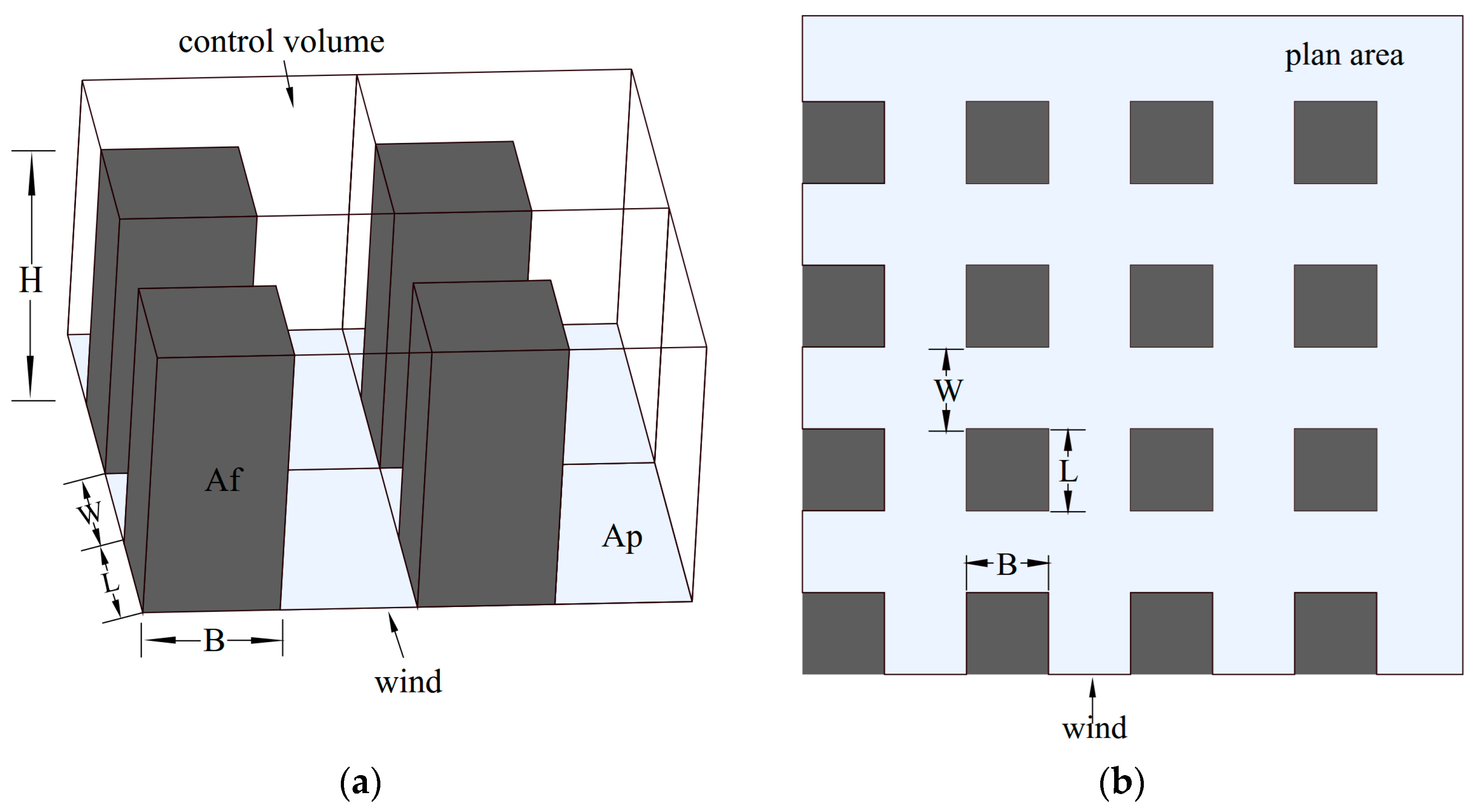
Figure 1. Geometric dimensions of building obstacles in the control volume. (a) perspective-view model sketch, (b) top view of the control volume.
Atmosphere 15 00352 g001
Figure 2. (a) Vertical cross-section in the domain of the canopy model for RANS simulation (14 rows) and wind tunnel experiment (7 rows). (b) The positions of vertical profiles of streamwise velocity in 4 canyons on the leeward side of the 1st, 3rd, 6th, and 7th obstacles. The profiles obtained at the same positions of the wind tunnel experiments are used for validation study.
Atmosphere 15 00352 g002
Figure 3. Vertical profiles of streamwise velocity at 4 points from wind-tunnel data and numerical predictions. Subplots (ad) are the profiles obtained at the location C1, C3, C6, C7, respectively.
Atmosphere 15 00352 g003
Figure 4. (a) Drag force coefficient (Cd) values across different model scales, from full size to wind tunnel scale, and variations of Cd under varying background wind speed (1–5 m/s at 15 m height) and building height: (b) H = 10 m, (c) H = 28 m, and (d) H = 63 m.
Atmosphere 15 00352 g004
Figure 5. (a) Total drag force per unit plan area with different λp, (b) mean streamwise wind velocity per unit plan area with different λp.
Atmosphere 15 00352 g005
Figure 6. Vertical distribution of streamwise velocity in different canopies with various λp: (a) λp = 0.16; (b) λp = 0.35; (c) λp = 0.51; (d) λp = 0.70.
Atmosphere 15 00352 g006
Figure 7. (ac) Variation in Cd, Cd·λf/H, Cd·λf with λf (for λp = 0.04~0.7); (df) Variation in Cd, Cd·λf/H, Cd·λf with SVF (for λp = 0.04~0.7).
Atmosphere 15 00352 g007
Figure 8. Variation in SVF with λf across all cases in Table 1.
Atmosphere 15 00352 g008
Figure 9. (ac) Contours of Cd, Cd·λf/H, and Cd·λf with varying λp and λf; (df) contours of Cd, Cd·λf/H, and Cd·λf with varying λp and SVF.
Atmosphere 15 00352 g009
Figure 10. (ag) Variation in Cd with AR for cases in Table 2; (h) variation in the increasing slope of Cd with building height.
Atmosphere 15 00352 g010
Table 1. Groups of rectangular block arrangements to test the response of Cd to λp, λf, and SVF.
SetλpB = L (m)W (m)H (m)λfSVFSetλpB = L (m)W (m)H (m)λfSVF
10.0452050.05 0.70 60.444020280.31 0.30
0.04520100.10 0.70 0.444020300.33 0.28
0.04520200.20 0.57 0.444020400.44 0.22
0.04520300.31 0.49 0.444020500.56 0.19
20.0882080.08 0.69 0.444020630.70 0.15
0.08820200.20 0.51 0.444020720.80 0.14
0.08820300.31 0.41 0.444020901.00 0.11
30.162030100.08 0.66 70.515020100.10 0.52
0.162030200.16 0.52 0.515020200.20 0.36
0.162030300.24 0.43 0.515020300.31 0.27
0.162030400.32 0.37 0.515020400.41 0.21
0.162030500.40 0.32 0.515020500.51 0.18
0.162030750.60 0.24 0.515020780.80 0.12
0.1620301000.80 0.19 0.515020981.00 0.10
0.1620301251.00 0.16 80.5863.820200.18 0.35
40.25202050.06 0.70 0.5863.820400.36 0.21
0.252020100.13 0.57 0.5863.820640.58 0.14
0.252020200.25 0.40 0.5863.820800.73 0.12
0.252020300.38 0.31 0.5863.8201000.91 0.10
0.252020400.50 0.25 0.5863.8201201.09 0.08
0.252020500.63 0.21 90.6583.2201200.94 0.08
0.252020640.80 0.17 0.6583.2201000.78 0.10
0.252020801.00 0.14 0.6583.220830.65 0.11
0.252020961.20 0.12 0.6583.220600.47 0.15
50.352920100.12 0.54 0.6583.220400.31 0.21
0.352920200.24 0.38 0.6583.220300.23 0.27
0.352920290.35 0.30 100.7102.420200.14 0.35
0.352920400.48 0.24 0.7102.420300.21 0.26
0.352920500.60 0.20 0.7102.420400.27 0.21
0.352920660.80 0.16 0.7102.420500.34 0.17
0.352920831.00 0.13 0.7102.420700.48 0.13
0.3529201001.21 0.11 0.7102.420102.40.70 0.09
60.444020100.11 0.52 0.7102.4201200.82 0.08
0.444020200.22 0.37 0.7102.4201400.96 0.07
Table 2. Groups of rectangular block arrangements to test the response of Cd to floor aspect ratio (for each group: B/L = 0.25, 0.5, 0.75, 1, 2, 3, 4).
Set1234567
λp0.160.250.350.440.440.510.58
W (m)30203020202020
H (m)10306628502040
Disclaimer/Publisher’s Note: The statements, opinions and data contained in all publications are solely those of the individual author(s) and contributor(s) and not of MDPI and/or the editor(s). MDPI and/or the editor(s) disclaim responsibility for any injury to people or property resulting from any ideas, methods, instructions or products referred to in the content.