


Downscaling of Regional Air Quality Model Using Gaussian Plume Model and Random Forest Regression


Abstract
1. Introduction
2. Data and Methods
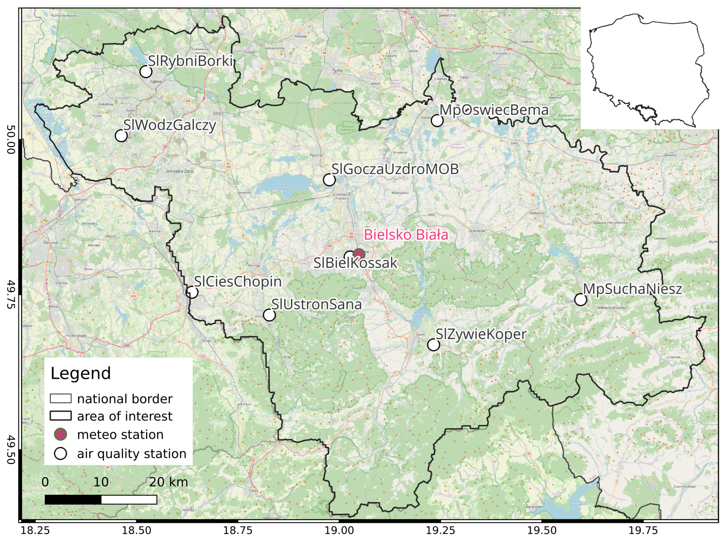
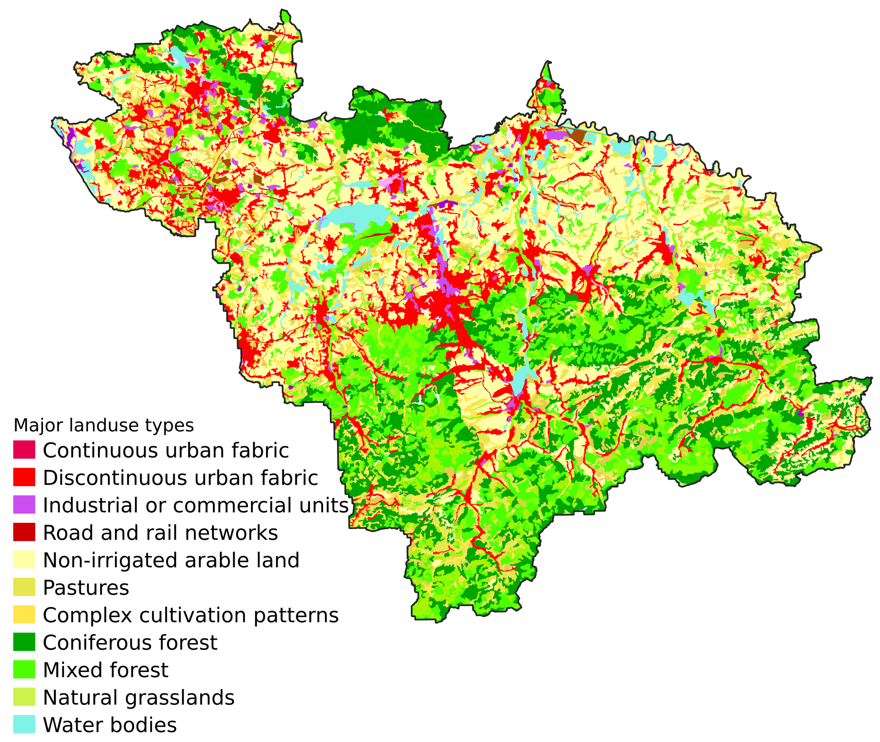
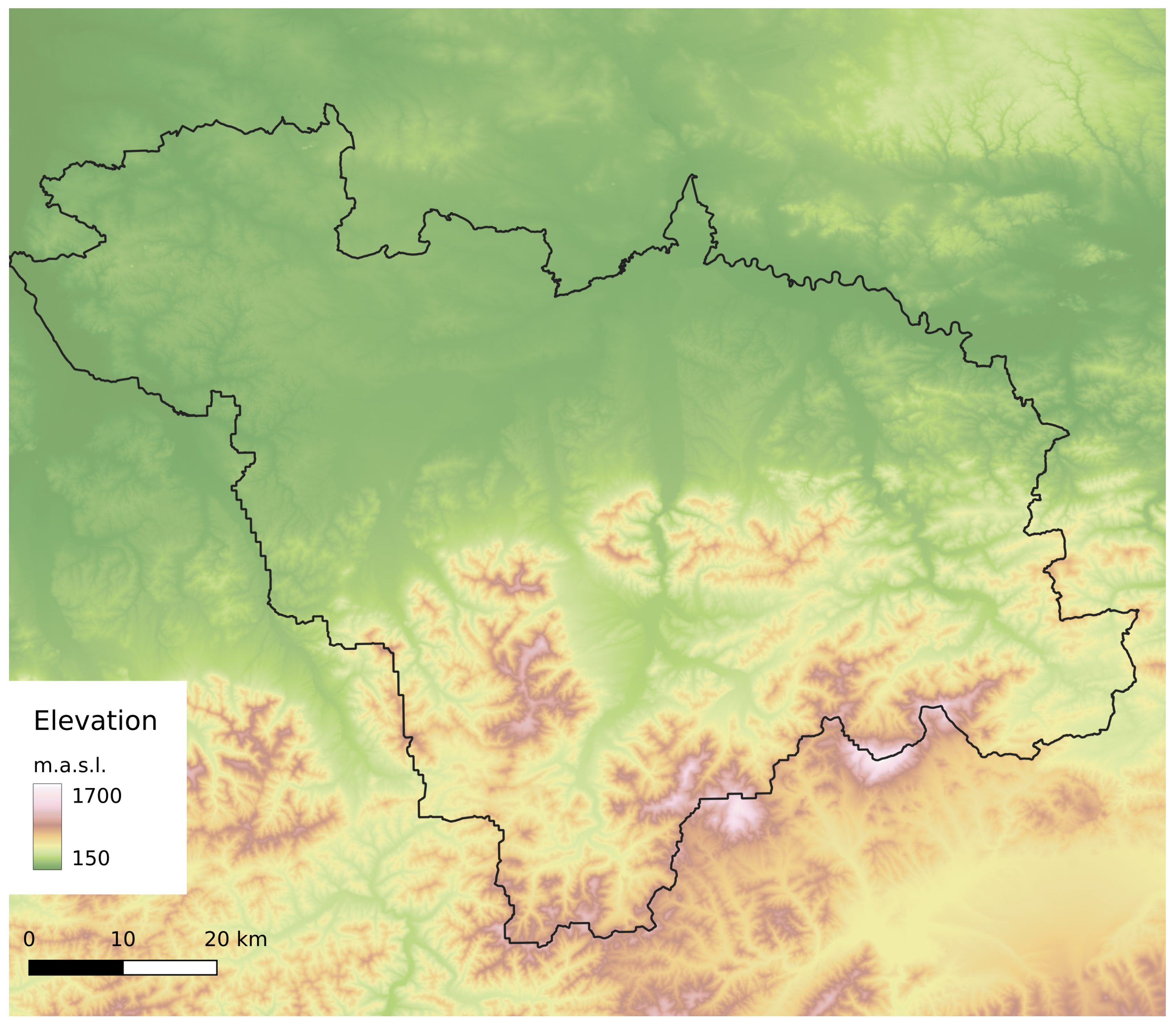
2.1. Study Area
2.2. The GEM-AQ Model
2.3. The Gaussian Plume Model
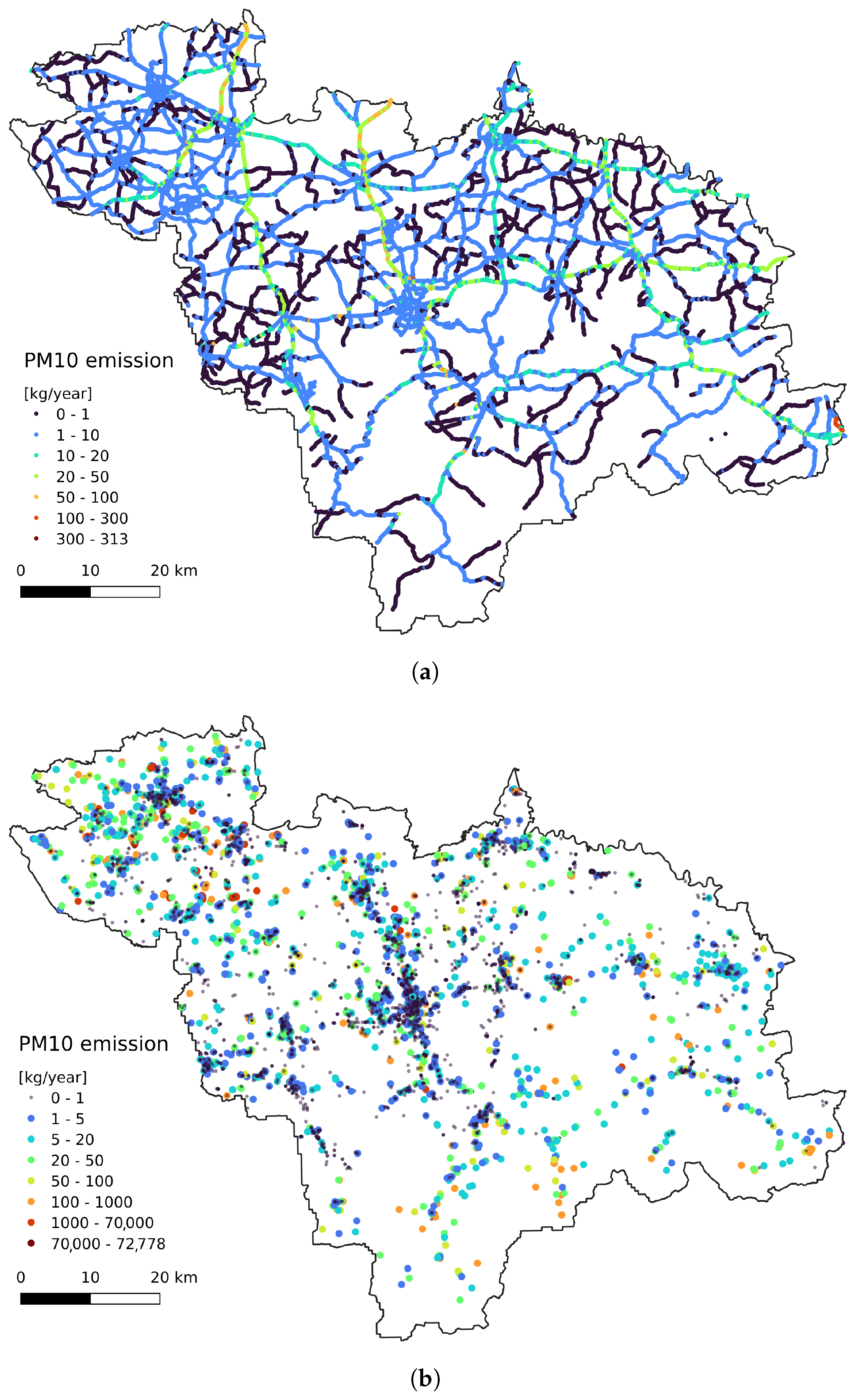
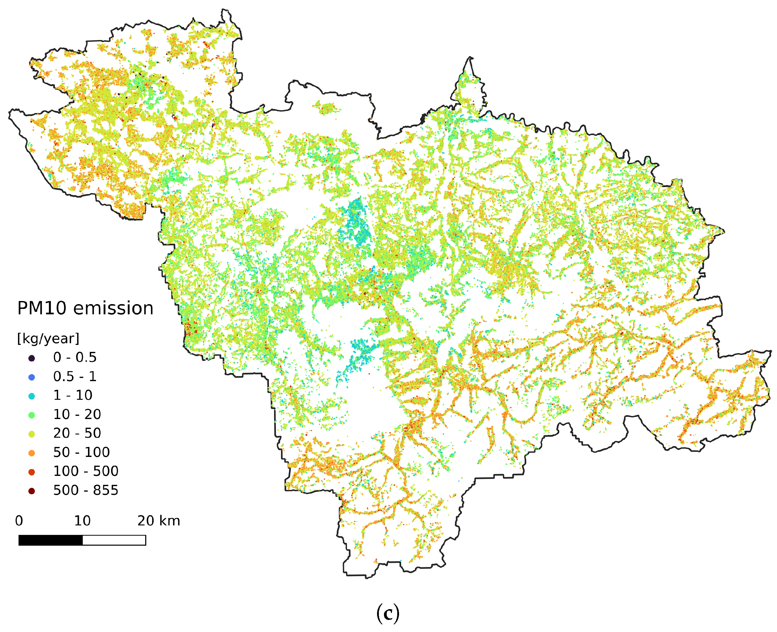
2.4. Emission Data
2.5. Surface Observations
2.6. Random Forest
3. Results
3.1. Overall Performance
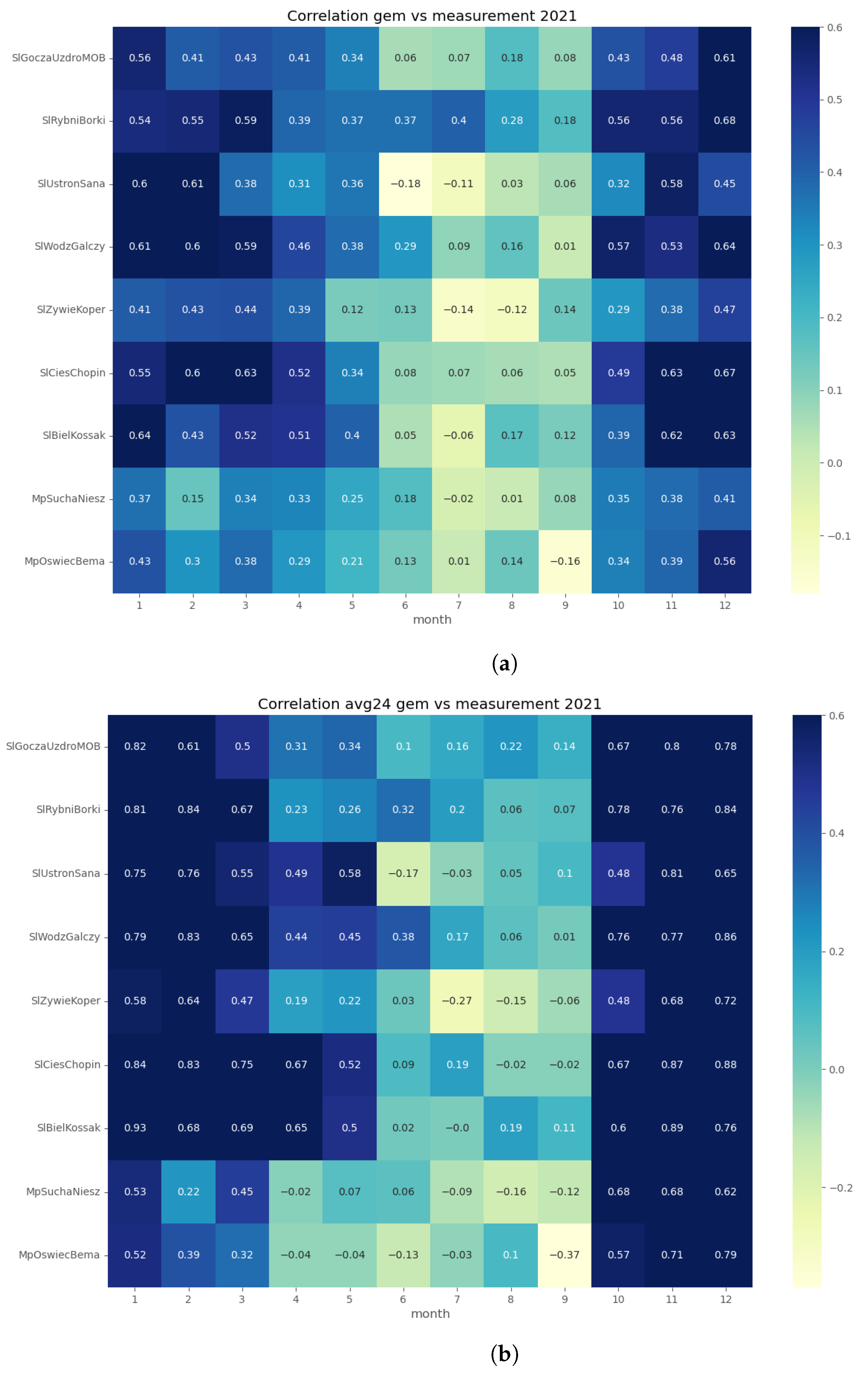
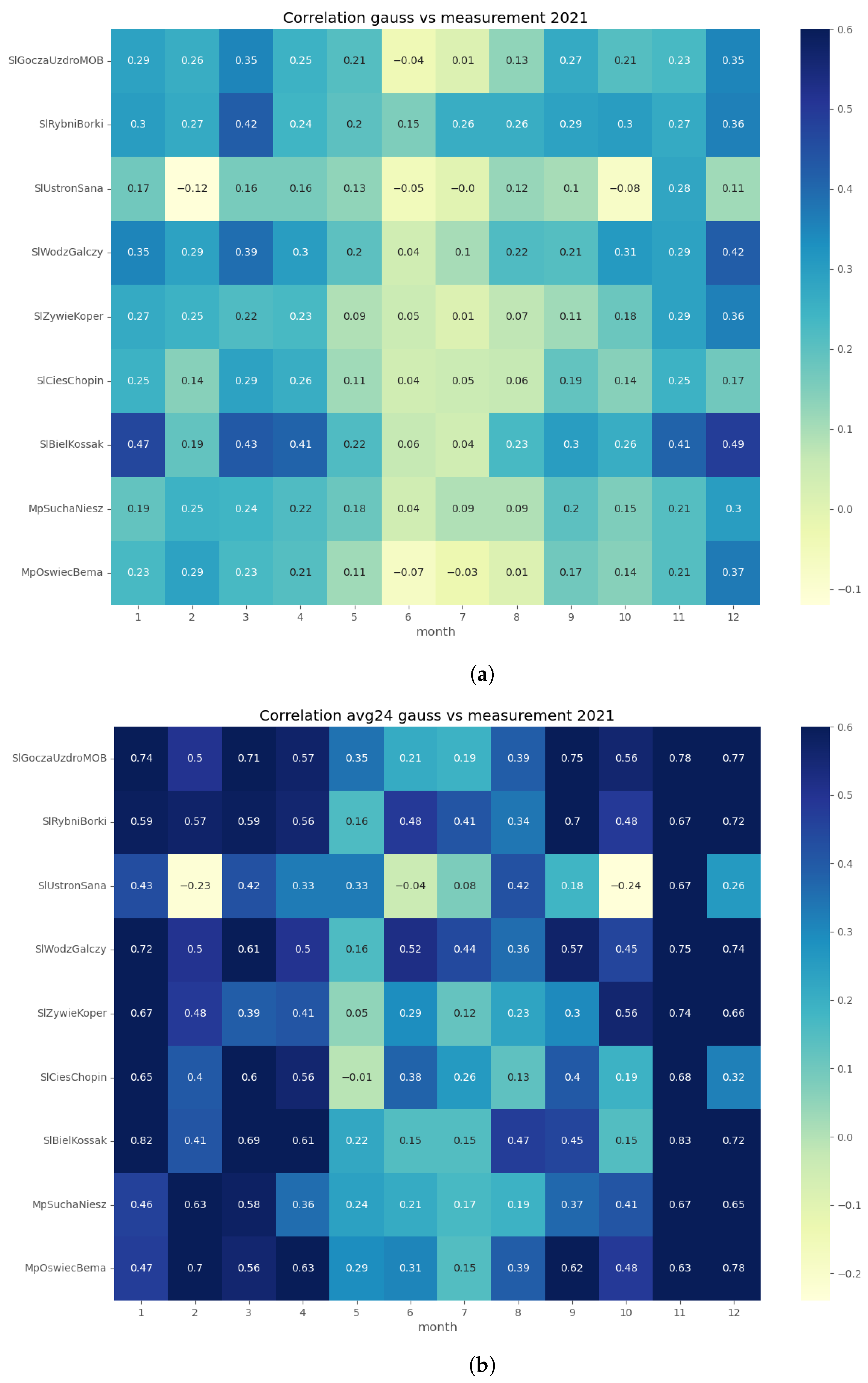
3.2. Temporal Comparison
3.3. Spatial Comparison
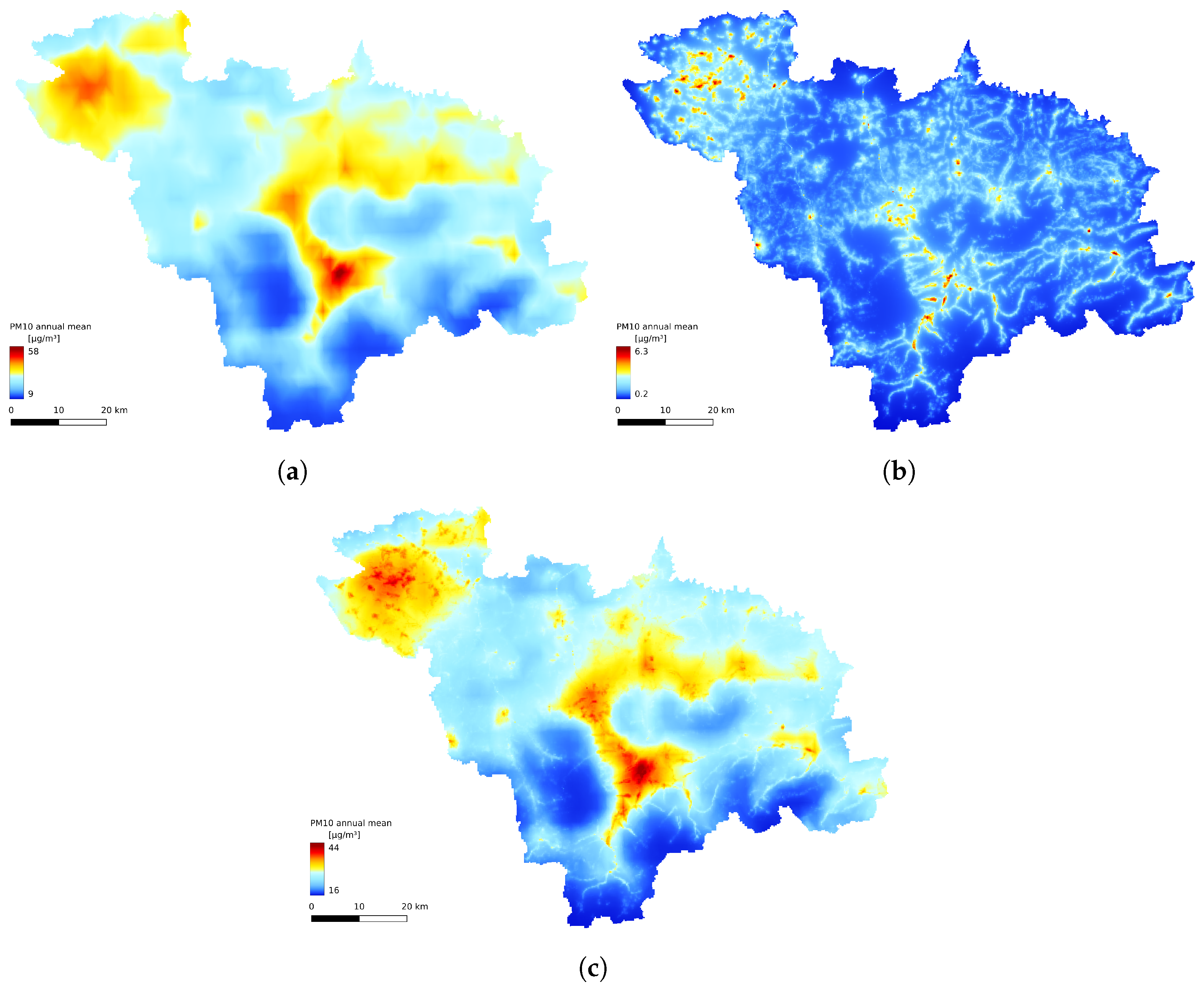
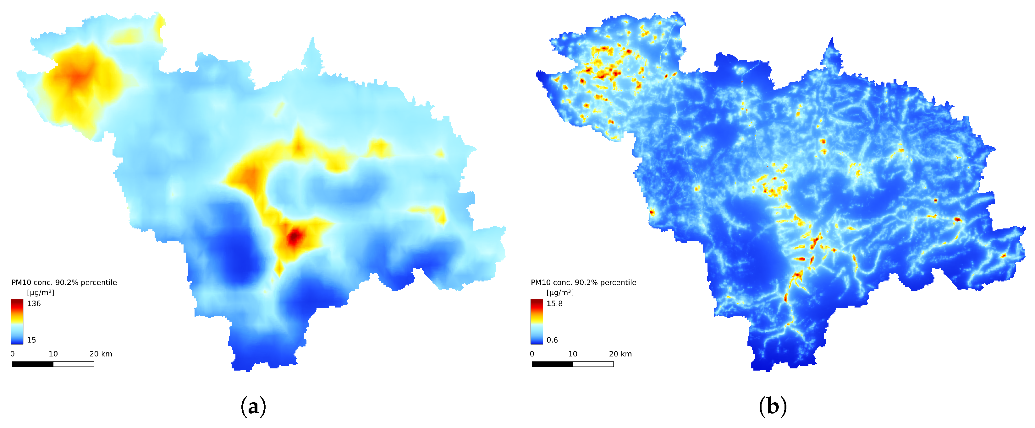
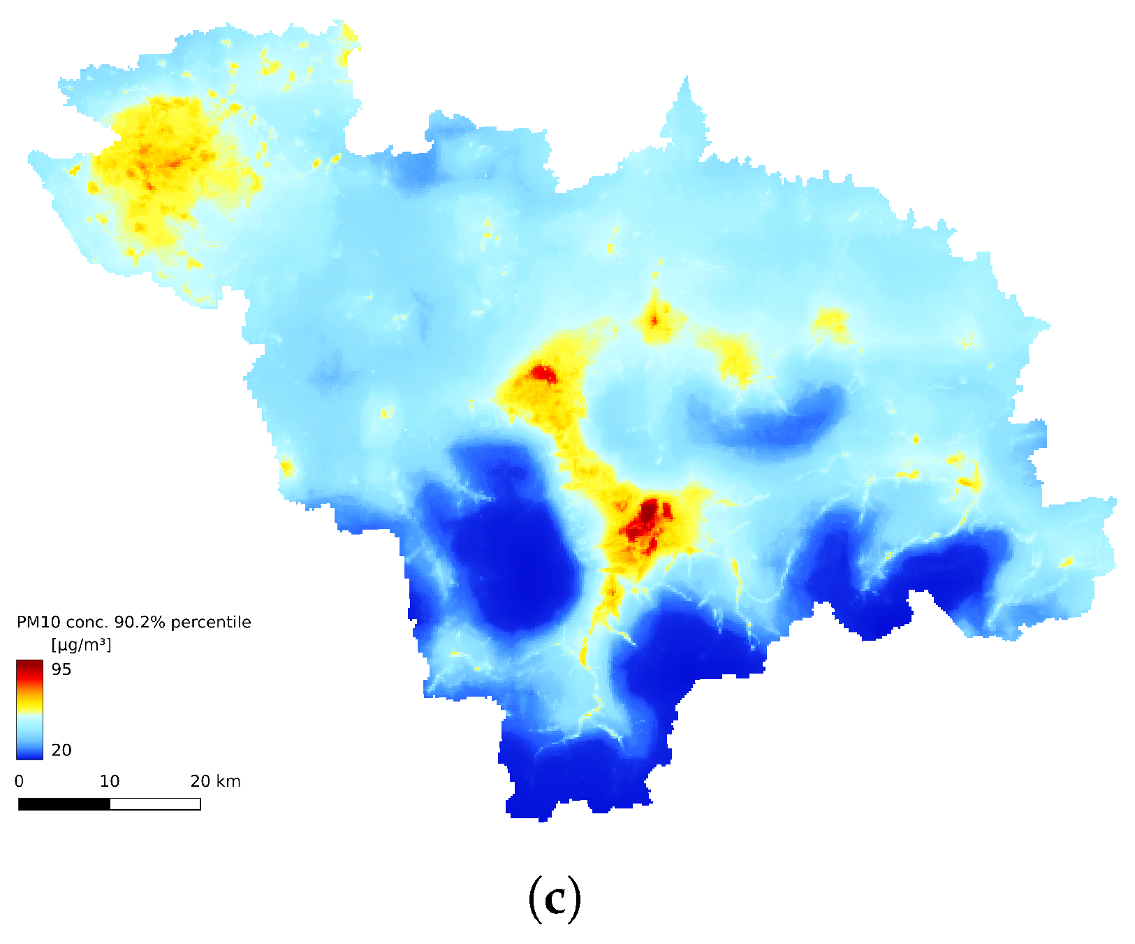
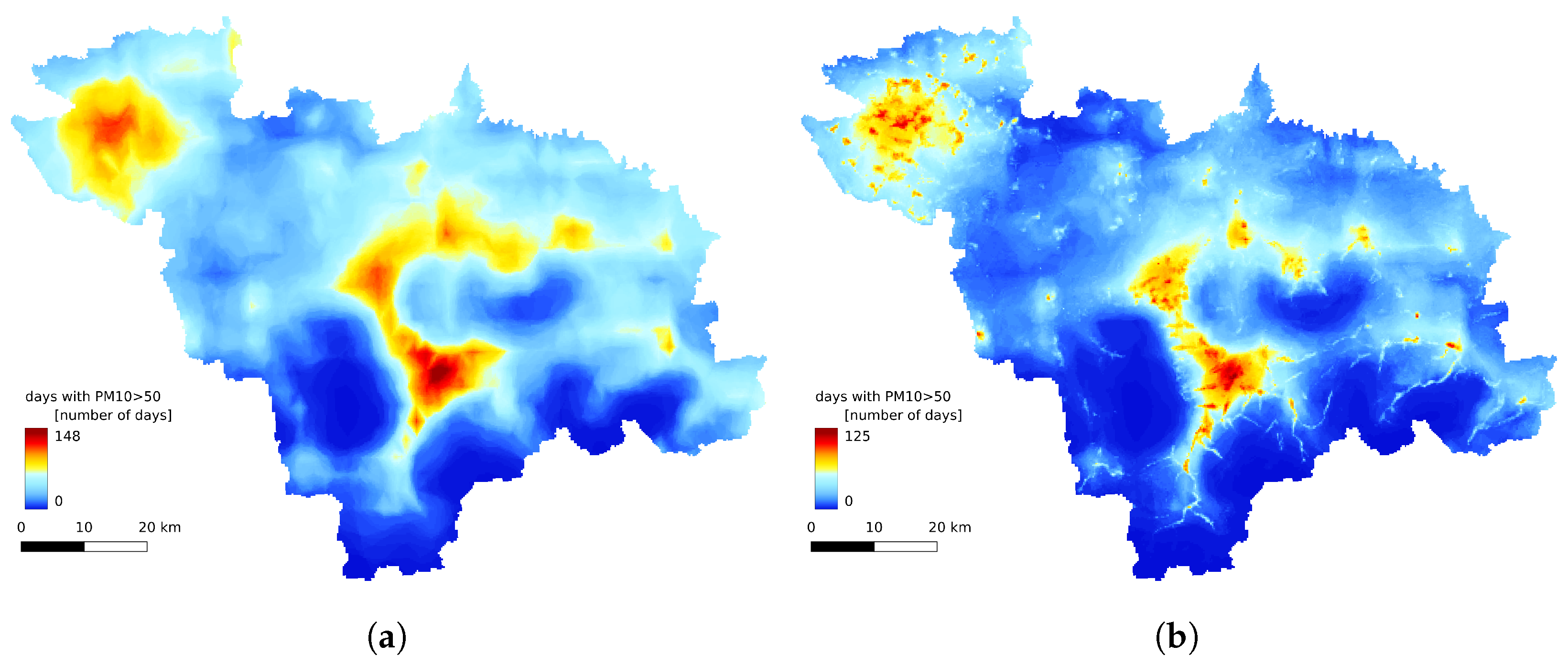
3.4. Annual Statistics
4. Discussion
5. Conclusions
Author Contributions
Funding
Institutional Review Board Statement
Informed Consent Statement
Data Availability Statement
Conflicts of Interest
Appendix A. Timeseries Evaluation
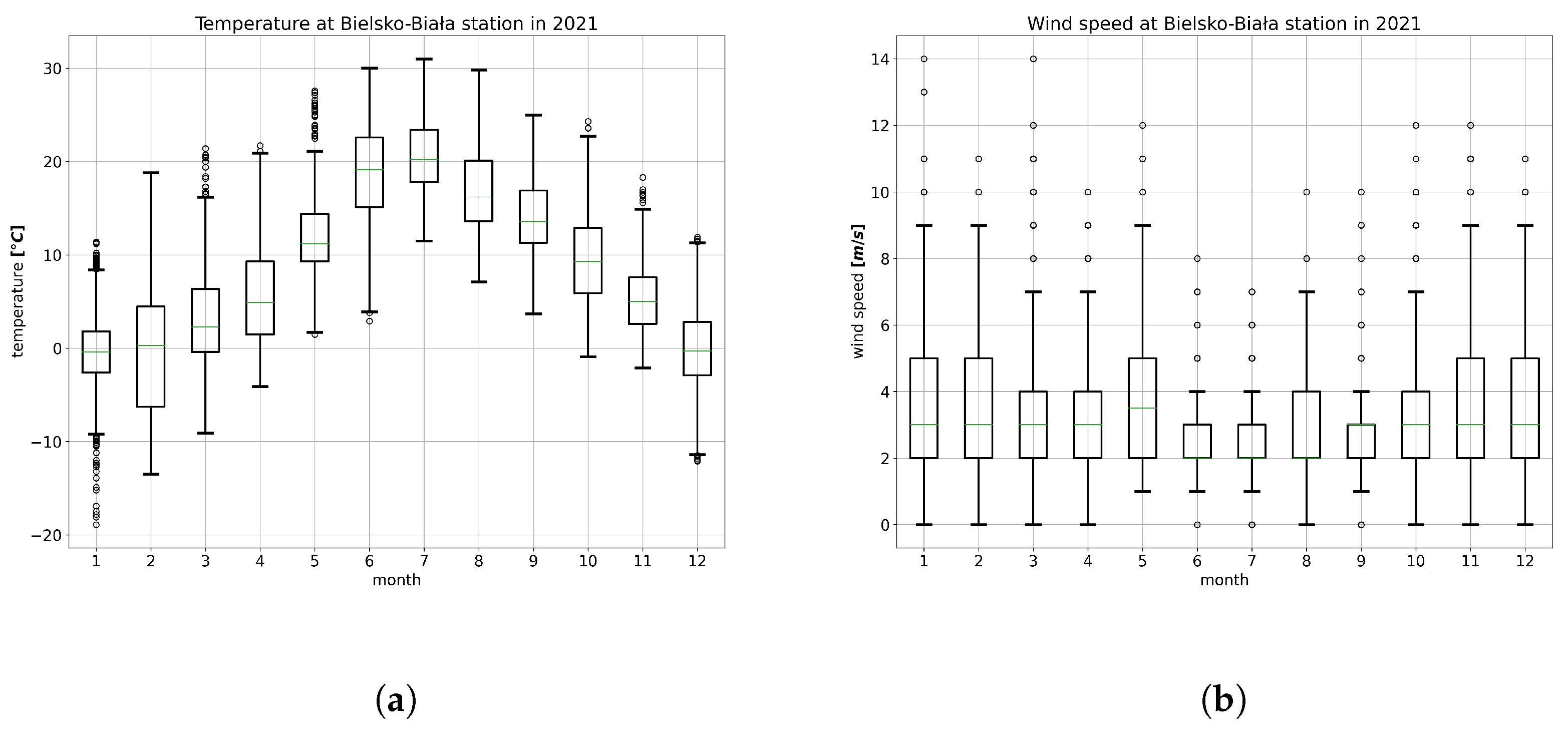
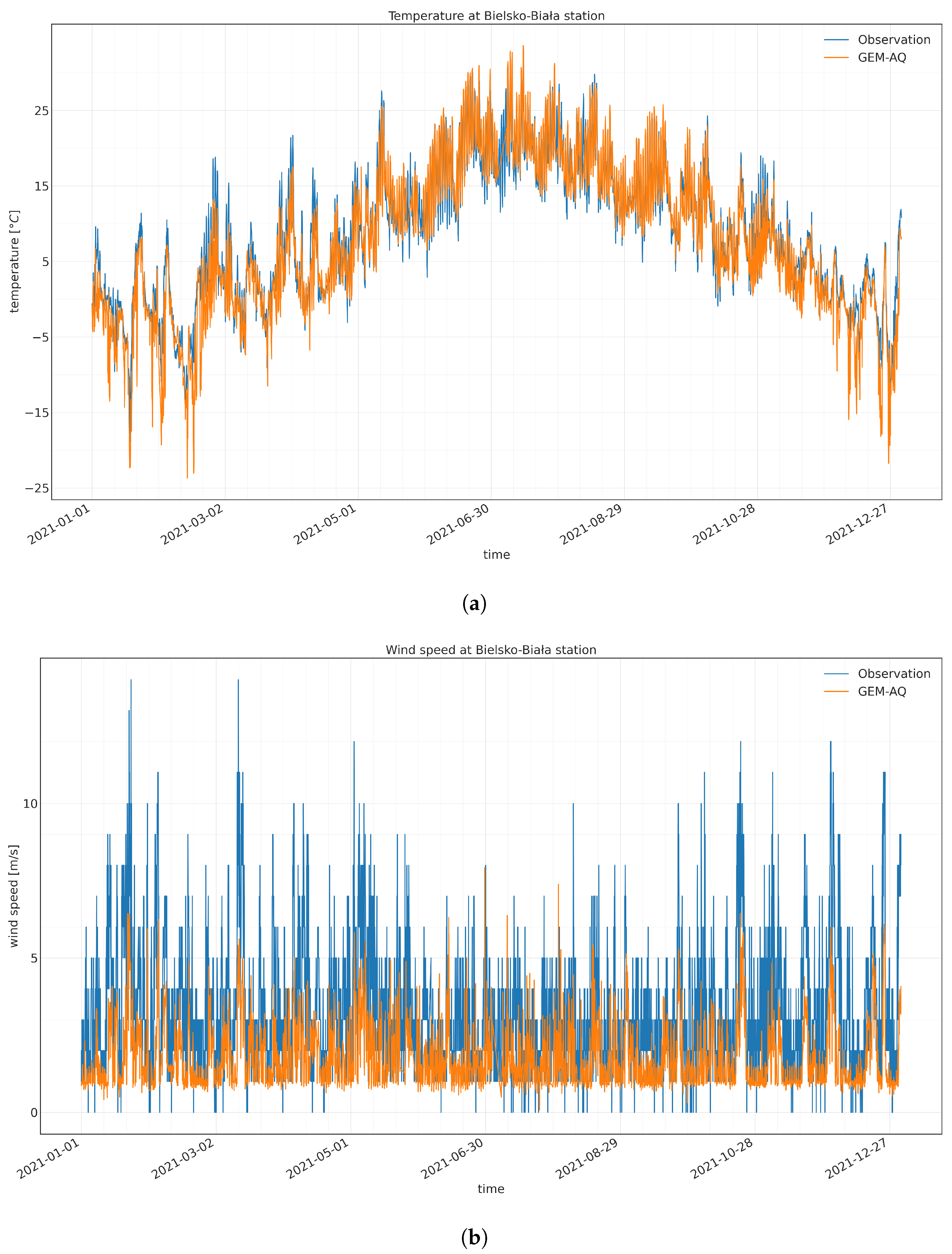
Appendix A.1. Meteorological Model Evaluation
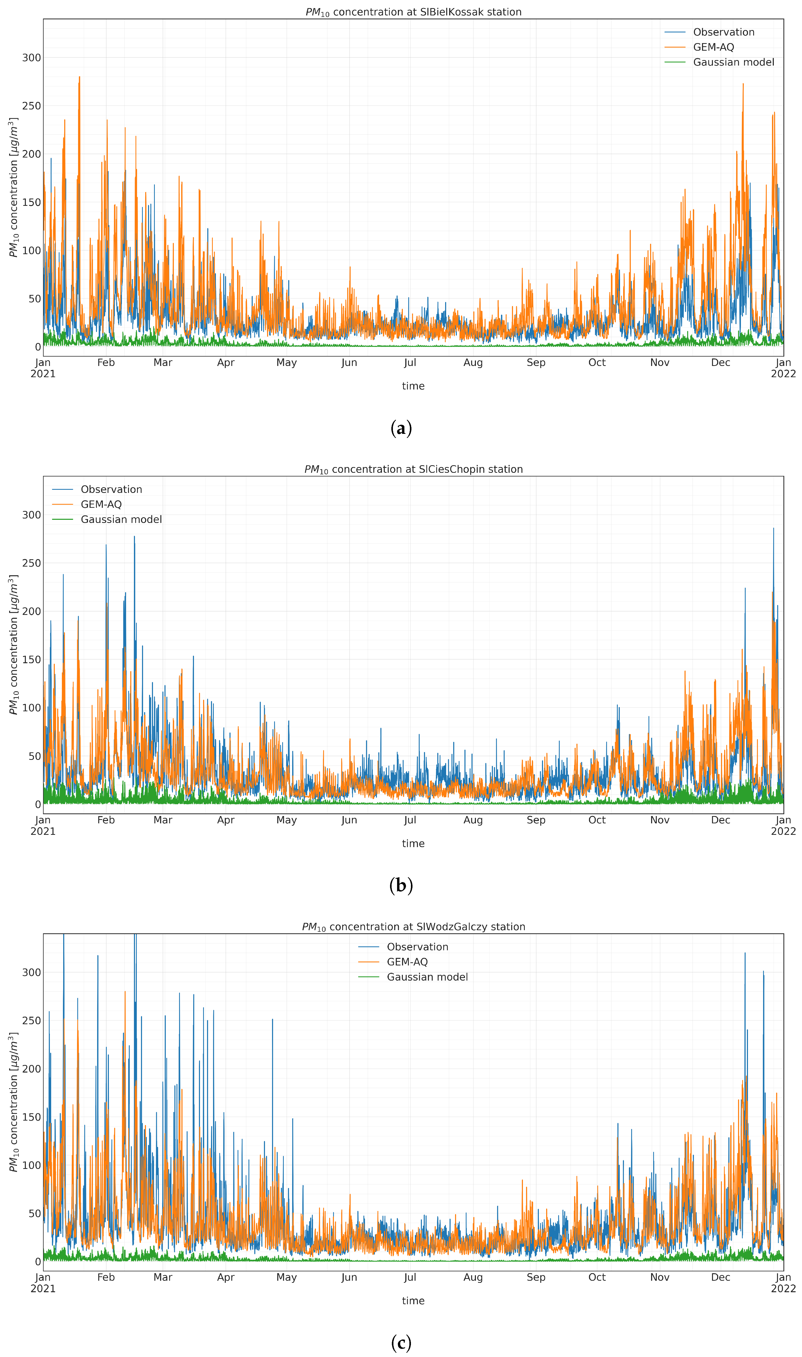
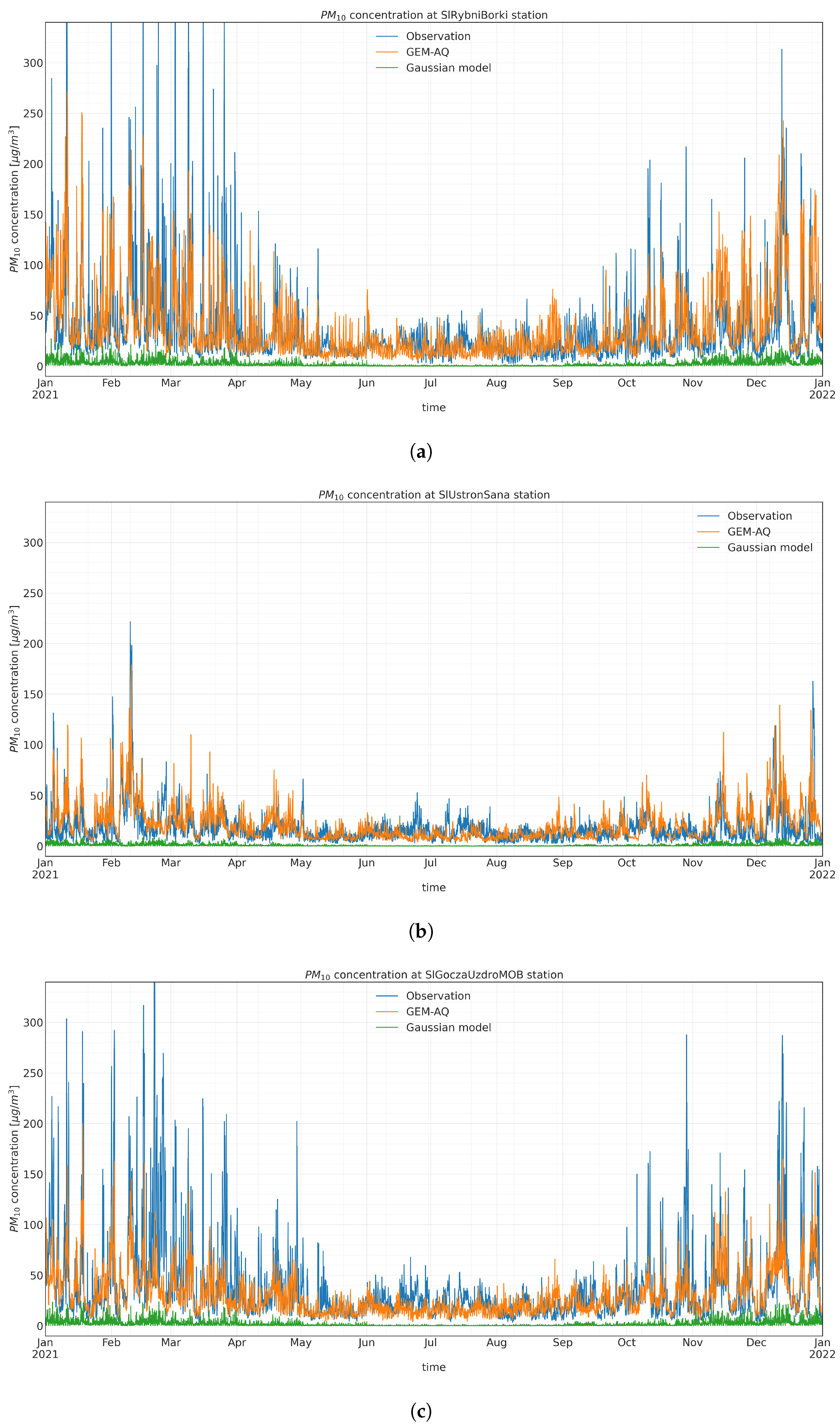
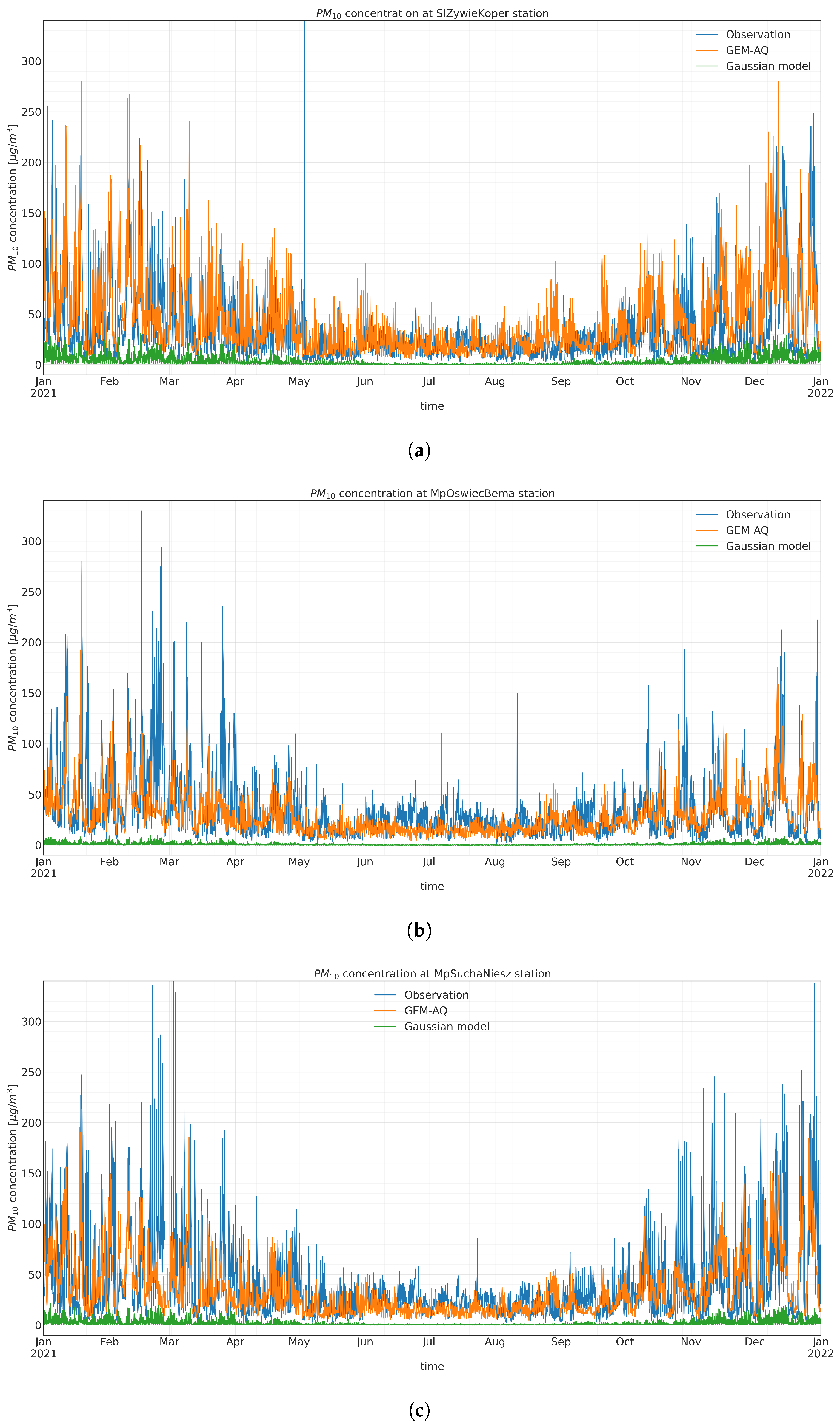
Appendix A.2. PM10 Input Time Series Evaluation
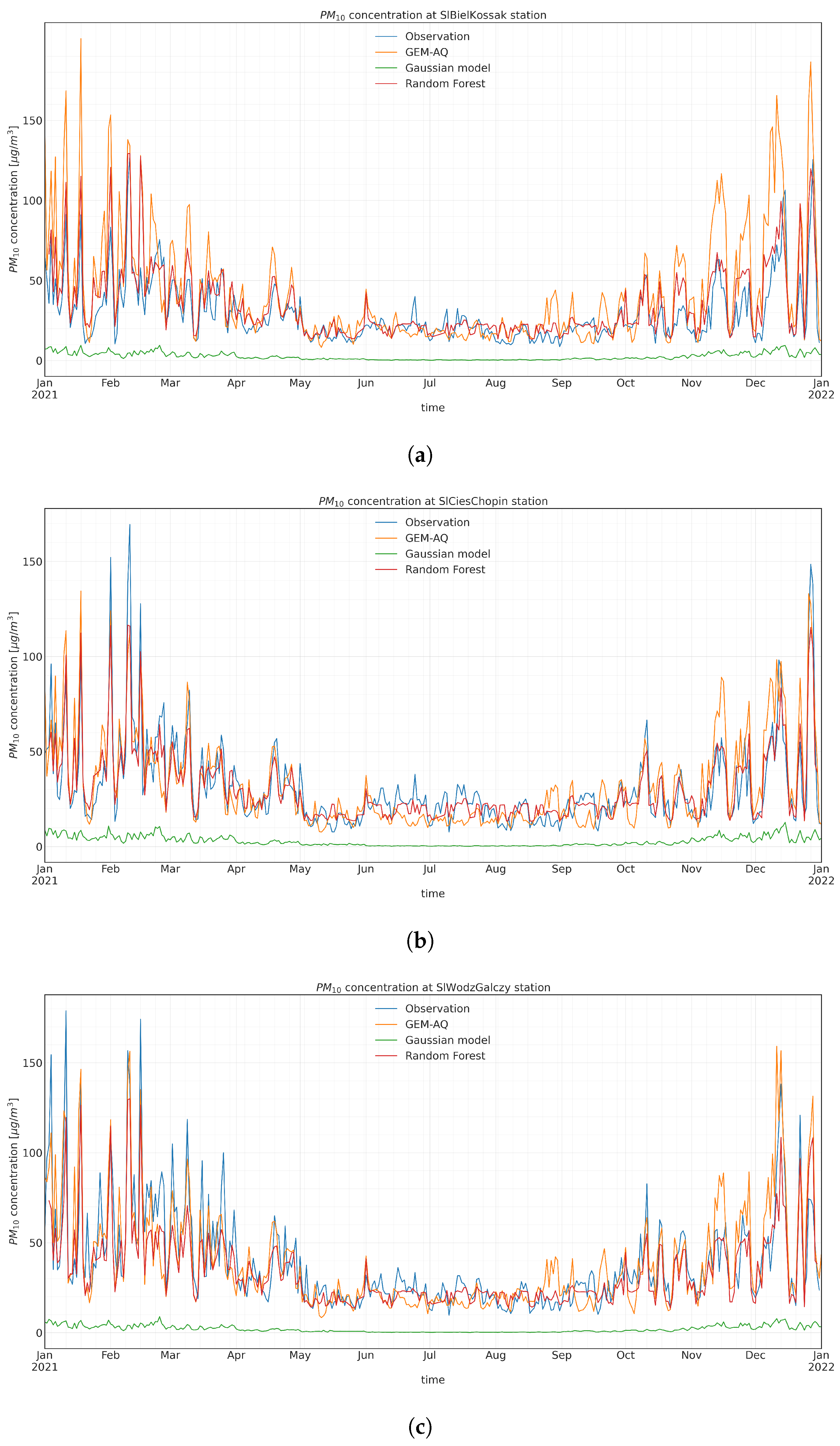
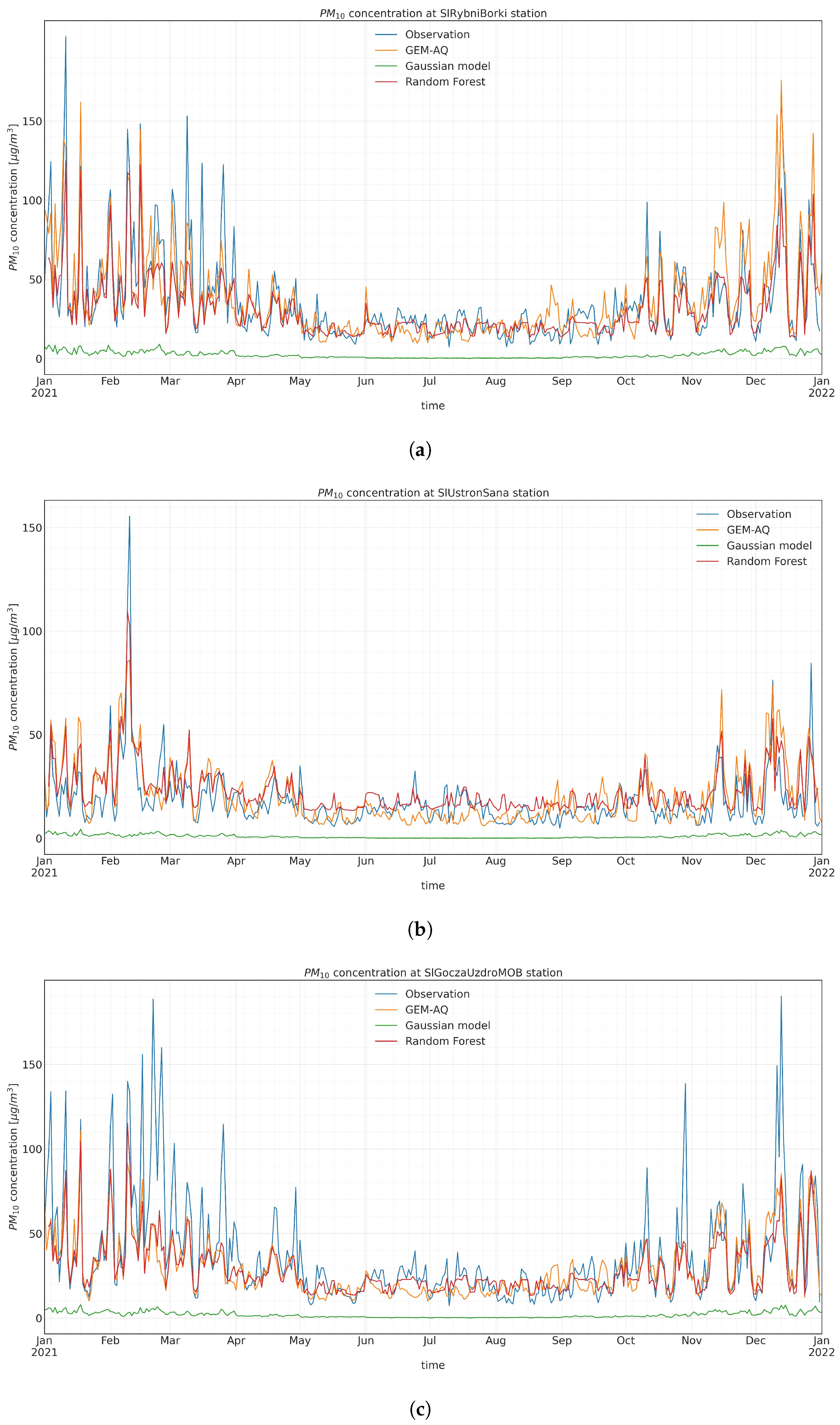
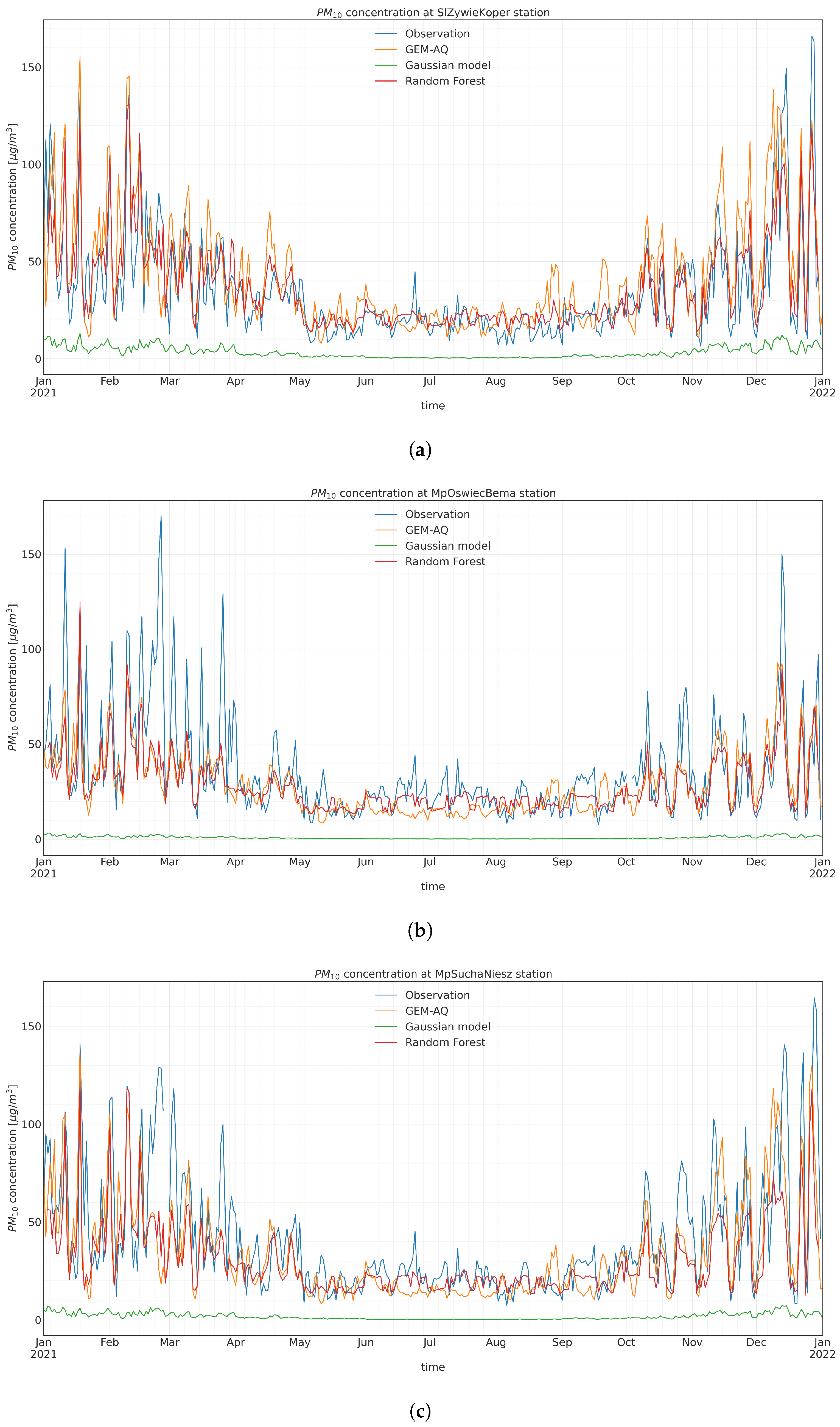
Appendix A.3. Random Forest Output PM 10 Time Series
References
- U.S. Environmental Protection Agency. Particulate Matter (PM) Basics. Available online: https://www.epa.gov/pm-pollution/particulate-matter-pm-basics (accessed on 1 July 2023).
- Jagiello, P.; Struzewska, J.; Jeleniewicz, G.; Kaminski, J.W. Evaluation of the Effectiveness of the National Clean Air Programme in Terms of Health Impacts from Exposure to PM2.5 and NO2 Concentrations in Poland. Int. J. Environ. Res. Public Health 2022, 20, 530. [Google Scholar] [CrossRef]
- Reizer, M.; Juda-Rezler, K. Explaining the high PM10 concentrations observed in Polish urban areas. Air Qual. Atmos. Health 2016, 9, 517–531. [Google Scholar] [CrossRef]
- Kobza, J.; Geremek, M.; Dul, L. Characteristics of air quality and sources affecting high levels of PM10 and PM2.5 in Poland, Upper Silesia urban area. Environ. Monit. Assess. 2018, 190, 515. [Google Scholar] [CrossRef]
- Emili, E.; Popp, C.; Petitta, M.; Riffler, M.; Wunderle, S.; Zebisch, M. PM10 remote sensing from geostationary SEVIRI and polar-orbiting MODIS sensors over the complex terrain of the European Alpine region. Remote Sens. Environ. 2010, 114, 2485–2499. [Google Scholar] [CrossRef]
- Alvarez-Mendoza, C.I.; Teodoro, A.C.; Torres, N.; Vivanco, V. Assessment of remote sensing data to model PM10 estimation in cities with a low number of air quality stations: A case of study in Quito, Ecuador. Environments 2019, 6, 85. [Google Scholar] [CrossRef]
- Park, J.; Lee, P.S.H. Relationship between Remotely Sensed Ambient PM10 and PM2.5 and Urban Forest in Seoul, South Korea. Forests 2020, 11, 1060. [Google Scholar] [CrossRef]
- Leelossy, Á.; Molnár, F.; Izsák, F.; Havasi, Á.; Lagzi, I.; Mészáros, R. Dispersion modeling of air pollutants in the atmosphere: A review. Open Geosci. 2014, 6, 257–278. [Google Scholar] [CrossRef]
- Veigele, W.J.; Head, J.H. Derivation of the Gaussian plume model. J. Air Pollut. Control Assoc. 1978, 28, 1139–1140. [Google Scholar] [CrossRef]
- Lutman, E.; Jones, S.; Hill, R.; McDonald, P.; Lambers, B. Comparison between the predictions of a Gaussian plume model and a Lagrangian particle dispersion model for annual average calculations of long-range dispersion of radionuclides. J. Environ. Radioact. 2004, 75, 339–355. [Google Scholar] [CrossRef]
- Rybarczyk, Y.; Zalakeviciute, R. Machine learning approaches for outdoor air quality modelling: A systematic review. Appl. Sci. 2018, 8, 2570. [Google Scholar] [CrossRef]
- Navares, R.; Aznarte, J.L. Predicting air quality with deep learning LSTM: Towards comprehensive models. Ecol. Inform. 2020, 55, 101019. [Google Scholar] [CrossRef]
- Kaminska, J.A. The use of random forests in modelling short-term air pollution effects based on traffic and meteorological conditions: A case study in Wrocław. J. Environ. Manag. 2018, 217, 164–174. [Google Scholar] [CrossRef] [PubMed]
- Ignaccolo, R.; Mateu, J.; Giraldo, R. Kriging with external drift for functional data for air quality monitoring. Stoch. Environ. Res. Risk Assess. 2014, 28, 1171–1186. [Google Scholar] [CrossRef]
- Liang, F.; Gao, M.; Xiao, Q.; Carmichael, G.R.; Pan, X.; Liu, Y. Evaluation of a data fusion approach to estimate daily PM2.5 levels in North China. Environ. Res. 2017, 158, 54–60. [Google Scholar] [CrossRef] [PubMed]
- Liu, J.; Li, T.; Xie, P.; Du, S.; Teng, F.; Yang, X. Urban big data fusion based on deep learning: An overview. Inf. Fusion 2020, 53, 123–133. [Google Scholar] [CrossRef]
- Sarigiannis, D.A.; Soulakellis, N.A.; Sifakis, N.I. Information fusion for computational assessment of air quality and health effects. Photogramm. Eng. Remote Sens. 2004, 70, 235–245. [Google Scholar] [CrossRef]
- Friberg, M.D.; Kahn, R.A.; Holmes, H.A.; Chang, H.H.; Sarnat, S.E.; Tolbert, P.E.; Russell, A.G.; Mulholland, J.A. Daily ambient air pollution metrics for five cities: Evaluation of data-fusion-based estimates and uncertainties. Atmos. Environ. 2017, 158, 36–50. [Google Scholar] [CrossRef]
- Kaminski, J.; Neary, L.; Struzewska, J.; McConnell, J.; Lupu, A.; Jarosz, J.; Toyota, K.; Gong, S.; Côté, J.; Liu, X.; et al. GEM-AQ, an on-line global multiscale chemical weather modelling system: Model description and evaluation of gas phase chemistry processes. Atmos. Chem. Phys. 2008, 8, 3255–3281. [Google Scholar] [CrossRef]
- Liu, B.; Ma, X.; Ma, Y.; Li, H.; Jin, S.; Fan, R.; Gong, W. The relationship between atmospheric boundary layer and temperature inversion layer and their aerosol capture capabilities. Atmos. Res. 2022, 271, 106121. [Google Scholar] [CrossRef]
- Côté, J.; Gravel, S.; Méthot, A.; Patoine, A.; Roch, M.; Staniforth, A. The operational CMC–MRB global environmental multiscale (GEM) model. Part I: Design considerations and formulation. Mon. Weather Rev. 1998, 126, 1373–1395. [Google Scholar] [CrossRef]
- Venkatram, A.; Karamchandani, P.; Misra, P. Testing a comprehensive acid deposition model. Atmos. Environ. (1967) 1988, 22, 737–747. [Google Scholar] [CrossRef]
- Nielsen, O.K. EMEP/EEA Air Pollutant Emission Inventory Guidebook 2013. Technical Guidance to Prepare National Emission Inventories; European Environment Agency: Copenhagen, Denmark, 2013.
- Tagaris, E.; Sotiropoulou, R.E.P.; Gounaris, N.; Andronopoulos, S.; Vlachogiannis, D. Effect of the Standard Nomenclature for Air Pollution (SNAP) categories on air quality over Europe. Atmosphere 2015, 6, 1119–1128. [Google Scholar] [CrossRef]
- Arystanbekova, N.K. Application of Gaussian plume models for air pollution simulation at instantaneous emissions. Math. Comput. Simul. 2004, 67, 451–458. [Google Scholar] [CrossRef]
- Briant, R.; Seigneur, C.; Gadrat, M.; Bugajny, C. Evaluation of roadway Gaussian plume models with large-scale measurement campaigns. Geosci. Model Dev. 2013, 6, 445–456. [Google Scholar] [CrossRef]
- Lotrecchiano, N.; Sofia, D.; Giuliano, A.; Barletta, D.; Poletto, M. Pollution dispersion from a fire using a Gaussian plume model. Int. J. Saf. Secur. Eng. 2020, 10, 431–439. [Google Scholar] [CrossRef]
- Kukkonen, J.; Nikmo, J.; Sofiev, M.; Riikonen, K.; Petäjä, T.; Virkkula, A.; Levula, J.; Schobesberger, S.; Webber, D. Applicability of an integrated plume rise model for the dispersion from wild-land fires. Geosci. Model Dev. 2014, 7, 2663–2681. [Google Scholar] [CrossRef]
- Stockie, J.M. The mathematics of atmospheric dispersion modeling. SIAM Rev. 2011, 53, 349–372. [Google Scholar] [CrossRef]
- Hanna, S.R.; Briggs, G.A.; Hosker, R.P., Jr. Handbook on Atmospheric Diffusion; Technical Report; National Oceanic and Atmospheric Administration: Oak Ridge, TN, USA, 1982.
- Davidson, G. A modified power law representation of the Pasquill-Gifford dispersion coefficients. J. Air Waste Manag. Assoc. 1990, 40, 1146–1147. [Google Scholar] [CrossRef]
- Mohan, M.; Siddiqui, T. Analysis of various schemes for the estimation of atmospheric stability classification. Atmos. Environ. 1998, 32, 3775–3781. [Google Scholar] [CrossRef]
- Carson, J.E.; Moses, H. The validity of several plume rise formulas. J. Air Pollut. Control Assoc. 1969, 19, 862–866. [Google Scholar] [CrossRef]
- Gawuc, L.; Szymankiewicz, K.; Kawicka, D.; Mielczarek, E.; Marek, K.; Soliwoda, M.; Maciejewska, J. Bottom–Up Inventory of Residential Combustion Emissions in Poland for National Air Quality Modelling: Current Status and Perspectives. Atmosphere 2021, 12, 1460. [Google Scholar] [CrossRef]
- Cutler, D.R.; Edwards, T.C., Jr.; Beard, K.H.; Cutler, A.; Hess, K.T.; Gibson, J.; Lawler, J.J. Random forests for classification in ecology. Ecology 2007, 88, 2783–2792. [Google Scholar] [CrossRef]
- Smith, P.F.; Ganesh, S.; Liu, P. A comparison of random forest regression and multiple linear regression for prediction in neuroscience. J. Neurosci. Methods 2013, 220, 85–91. [Google Scholar] [CrossRef]
- Breiman, L. Random forests. Mach. Learn. 2001, 45, 5–32. [Google Scholar] [CrossRef]
- Pearce, J.L.; Beringer, J.; Nicholls, N.; Hyndman, R.J.; Tapper, N.J. Quantifying the influence of local meteorology on air quality using generalized additive models. Atmos. Environ. 2011, 45, 1328–1336. [Google Scholar] [CrossRef]
- Werner, M.; Kryza, M.; Ojrzyńska, H.; Skjøth, C.A.; WałBszek, K.; Dore, A.J. Application of WRF-Chem to forecasting PM10 concentration over Poland. Int. J. Environ. Pollut. 2015, 58, 280–292. [Google Scholar] [CrossRef]
- Kicińska, A.; Mamak, M. Health risks associated with municipal waste combustion on the example of Laskowa commune (Southern Poland). Hum. Ecol. Risk Assess. Int. J. 2017, 23, 2087–2096. [Google Scholar] [CrossRef]
- Wojdyga, K.; Chorzelski, M.; Rozycka-Wronska, E. Emission of pollutants in flue gases from Polish district heating sources. J. Clean. Prod. 2014, 75, 157–165. [Google Scholar] [CrossRef]


| Stability Class | ||||||
|---|---|---|---|---|---|---|
| A | 0.22 | 0.0001 | −0.5 | 0.20 | 0.0 | 0.0 |
| B | 0.16 | 0.0001 | −0.5 | 0.12 | 0.0 | 0.0 |
| C | 0.11 | 0.0001 | −0.5 | 0.08 | 0.0002 | −0.5 |
| D | 0.08 | 0.0001 | −0.5 | 0.06 | 0.0015 | −0.5 |
| E | 0.06 | 0.0001 | −0.5 | 0.03 | 0.0003 | −1.0 |
| F | 0.04 | 0.0001 | −0.5 | 0.016 | 0.003 | −1.0 |
| Observation Station | Mean Concentration | 90.2% Concentration Percentile | No. of Days with a Concentration Exceeding 50 |
|---|---|---|---|
| MpOswiecBema | 35.81 | 72.32 | 69 |
| MpSuchaNiesz | 40.9 | 90.6 | 98 |
| SlBielKossak | 29.21 | 52.18 | 48 |
| SlCiesChopin | 31.0 | 56.91 | 54 |
| SlGoczaUzdroMOB | 37.27 | 78.88 | 77 |
| SlRybniBorki | 35.94 | 69.43 | 64 |
| SlUstronSana | 18.03 | 31.62 | 8 |
| SlWodzGalczy | 38.8 | 73.79 | 91 |
| SlZywieKoper | 34.54 | 64.83 | 66 |
| Target Variable | No Additional Features | Day of the Week, Month | Day of the Week, Month, Observed Wind, Observed Temperature | |
|---|---|---|---|---|
| hourly concentration | 0.28 | 0.34 | 0.37 | |
| 44.9 | 48.6 | 48.7 | ||
| daily mean concentration | 0.49 | 0.54 | 0.61 | |
| 62.8 | 65.5 | 68.1 | ||
| daily median concentration | 0.43 | 0.46 | 0.55 | |
| 59.9 | 62.6 | 66.0 | ||
| daily maximum concentration | 0.43 | 0.45 | 0.48 | |
| 57.8 | 59.7 | 60.3 |
| Hourly Concentration | Daily Mean | ||||
|---|---|---|---|---|---|
| January | 45 | 0.21 | January | 61 | 0.36 |
| February | 40 | 0.15 | February | 53 | 0.25 |
| March | 46 | 0.17 | March | 59 | 0.17 |
| April | 52 | 0.14 | April | 70 | 0.06 |
| May | 55 | 0.04 | May | 72 | 0.2 |
| June | 64 | 0.02 | June | 78 | 0.02 |
| July | 57 | 0 | July | 71 | −0.07 |
| August | 50 | 0.02 | August | 70 | 0.05 |
| September | 51 | 0.04 | September | 68 | −0.04 |
| October | 44 | 0.13 | October | 60 | 0.14 |
| November | 48 | 0.23 | November | 65 | 0.44 |
| December | 39 | 0.31 | December | 57 | 0.49 |
| Hourly Concentration | Daily Mean | ||||
|---|---|---|---|---|---|
| SlBielKossak | 60 | 0.5 | 72 | 0.64 | |
| SlWodzGalczy | 56 | 0.46 | 71 | 0.63 | |
| SlRybniBorki | 51 | 0.39 | 66 | 0.51 | |
| SlCiesChopin | 48 | 0.43 | 69 | 0.72 | |
| SlUstronSana | 49 | 0.35 | 66 | 0.51 | |
| SlGoczaUzdroMOB | 50 | 0.36 | 62 | 0.53 | |
| SlZywieKoper | 37 | 0.41 | 62 | 0.54 | |
| MpSuchaNiesz | 34 | 0.37 | 59 | 0.59 | |
| MpOswiecBema | 44 | 0.3 | 58 | 0.39 |
Disclaimer/Publisher’s Note: The statements, opinions and data contained in all publications are solely those of the individual author(s) and contributor(s) and not of MDPI and/or the editor(s). MDPI and/or the editor(s) disclaim responsibility for any injury to people or property resulting from any ideas, methods, instructions or products referred to in the content. |
© 2023 by the authors. Licensee MDPI, Basel, Switzerland. This article is an open access article distributed under the terms and conditions of the Creative Commons Attribution (CC BY) license (https://creativecommons.org/licenses/by/4.0/).
Share and Cite
Kawka, M.; Struzewska, J.; Kaminski, J.W. Downscaling of Regional Air Quality Model Using Gaussian Plume Model and Random Forest Regression. Atmosphere 2023, 14, 1171. https://doi.org/10.3390/atmos14071171
Kawka M, Struzewska J, Kaminski JW. Downscaling of Regional Air Quality Model Using Gaussian Plume Model and Random Forest Regression. Atmosphere. 2023; 14(7):1171. https://doi.org/10.3390/atmos14071171
Chicago/Turabian StyleKawka, Marcin, Joanna Struzewska, and Jacek W. Kaminski. 2023. "Downscaling of Regional Air Quality Model Using Gaussian Plume Model and Random Forest Regression" Atmosphere 14, no. 7: 1171. https://doi.org/10.3390/atmos14071171
APA StyleKawka, M., Struzewska, J., & Kaminski, J. W. (2023). Downscaling of Regional Air Quality Model Using Gaussian Plume Model and Random Forest Regression. Atmosphere, 14(7), 1171. https://doi.org/10.3390/atmos14071171