Article

Downscaling and Wind Resource Assessment of Climatic Wind Speed Data Based on Deep Learning: A Case Study of the Tengger Desert Wind Farm

1
Economic Transformation of Climate Resources Key Laboratory, China Meteorological Administration, Chongqing 401120, China
2
Chongqing Shete Meteorological Application Research Institute, Chongqing Meteorological Service, Chongqing 401120, China
3
Haizhuang Wind Power Co., Ltd., China State Shipbuilding Corp (CSSC), Chongqing 401120, China
*
Authors to whom correspondence should be addressed.
Atmosphere 2024, 15(3), 271; https://doi.org/10.3390/atmos15030271
Submission received: 8 January 2024 / Revised: 16 February 2024 / Accepted: 20 February 2024 / Published: 24 February 2024
(This article belongs to the Topic Wind, Wave and Tidal Energy Technologies in China)

Abstract

:
Analyzing historical and reanalysis datasets for wind energy climatic characteristics offers crucial insights for wind farms and short-term electricity generation forecasting. However, large-scale wind farms in Chinese deserts, the Gobi, and barren areas often lack sufficient wind measurement data, leading to challenges in assessing long-term power generation revenue and introducing uncertainty. This study focuses on the Tengger Desert as the study area, processes the Coupled Model Intercomparison Project Phase 6 (CMIP6) data, and analyzes and compares wind energy’s future characteristics utilizing a developed deep learning (DL) downscaling algorithm. The findings indicate that (1) the Convolutional Neural Network (CNN) downscaling model, with the Weather Research and Forecasting Model (WRF) numerical simulation results as the targets, exhibits spatial distribution consistency with WRF simulation results in the experimental area. (2) Through testing and validation with three practical wind measurements, the annual average wind speed error is below 4%. (3) In the mid-term future (~2050), the average wind speed in the experimental area remains stable with a multi-year average of approximately 7.00 m·s−1. The overall wind speed distribution range is significant, meeting the requirements for wind farm development.

1. Introduction

The deserts, Gobi, and barren lands in the northern regions of China constitute a promising area for onshore renewable energy development, particularly in wind power. Due to the rapid growth of wind power in this region, many yet-to-be-developed wind farms often lack wind measurement towers or are constrained by a limited number of such buildings. The traditional wind resource assessment with meteorological towers relies primarily on installing measurement towers at specific locations to observe and collect wind speed and wind direction data. Although this method is directly effective, it often fails to accurately assess the overall wind conditions across the entire wind farm area due to the limited number and representativeness of measurement points. Furthermore, meteorological tower construction and maintenance costs are relatively high, and reliable results require long-term observations.
Wind farms typically have a construction period of one year and an operational lifespan of 20 years. Over the next few decades, wind farms’ long-term electricity generation revenue will also face the uncertain challenge of changes in wind energy resources [1], such as urbanization and land cover changes, which significantly impact the long-term variations in land surface wind speeds. However, the scientific community acknowledges that natural and anthropogenic interactions and forcings within the Earth’s climate system greatly influence surface wind speed. Previous studies have indicated that land surface wind speeds have generally decreased in most regions of the Northern Hemisphere, including Europe (0.01–0.09 m·s−1·decade−1), the United States (0.10–0.19 m·s−1·decade−1), and China (0.12–0.22 m·s−1·decade−1) over the past few decades [2,3,4,5,6].
Global Climate Models (GCMs) have been widely utilized to generate predictions of climate change and weather event patterns related to land surface winds [1,7]. Under the auspices of the World Climate Research Programme (WCRP) Coupled Model Intercomparison Project (CMIP), the global modeling centers conducted the GCM experiments. They shared their simulation results [8]. The latest phase of the Coupled Model Intercomparison Project (CMIP), initiated in 2015 (CMIP6), provides the most advanced multi-model datasets and is one of the most effective tools for enhancing our understanding and forecasting of climate change [9]. These model datasets encompass a range of historical simulations and future scenario experiments. Historical simulation data based on observational records (1850 to 2014) is commonly employed to assess the ability to simulate climate variability and analyze the causes of forced climate change [10]. Moreover, the GCMs provide corresponding future scenarios by specifying greenhouse gas and aerosol concentrations, enabling the setup of different future scenario experiments to help predict potential climate changes in the future. With the assistance of GCMs, understanding of past, present, and future climate change has been enhanced.
The prediction of future wind energy resources is based on the previous phases of the CMIP6 implementation. For the prediction of future wind resources in the upcoming periods, CMIP6 has been extensively utilized in studies related to monsoon variability [11], offshore wind energy resources [12,13,14], onshore wind resources [15], and others. However, the spatial resolution of CMIP6 is 100 km, which is too coarse to provide actionable information for the study of local wind energy resources. Therefore, there is a need to enhance the spatial resolution of CMIP6 for more effective environmental research. The commonly used dynamic downscaling process with high-resolution Regional Climate Models (RCMs) is time-consuming and introduces additional uncertainties [16]. Spatiotemporal statistical downscaling is a practical approach for obtaining high-resolution data. This method is based on establishing correlations between the predictor variable (e.g., wind speed) and environmental variables (predictors) and then using finer-scale predictor variables as input to downscale the predictor variable from coarse resolution to finer resolution [17,18,19]. Due to its ease of implementation, fast computational speed, and low time consumption, statistical downscaling methods have been widely applied in climate change predictions [20,21].
Statistical downscaling methods can be broadly categorized into two types: linear methods, such as multiple linear regression, canonical correlation analysis, singular value decomposition, and model output statistics, and nonlinear methods, such as Convolutional Neural Networks (CNN) and stochastic weather generators [22]. Due to the complex terrain distribution, surface-atmosphere interactions, and thermodynamic processes in the boundary layer in the deserts, Gobi, and barren areas of the northern region of China, the empirical relationship between near-surface wind fields and large-scale climate variations exhibits numerous intricate features. Therefore, local near-surface winds are influenced by currently relevant large-scale and past and future predictor variables. These features pose significant challenges to traditional methods and constrain the achievement of high-quality downscaling processes. This study proposes a novel downscaling method based on deep learning (DL) networks to address this issue and ensure wind turbines’ safe and stable operation in extreme weather conditions over many years. In recent years, DL technology has been increasingly introduced and applied in earth system science and the wind energy industry [23]. The new downscaling method based on DL (CNN) can overcome the limitations in the number of hidden layers and neurons found in classical CNNs and incorporates fundamental differences in the training mechanism of deep networks. DL exhibits significant advantages in non-linear function approximation for data mining, feature extraction, and various levels of precision [24], making it considered an efficient method for handling and analyzing the ‘big data’ of climate in CMIP projects. However, DL methods still face several challenges. It typically requires large-scale annotated data to achieve good performance. Training DL models demands substantial computational resources. The DL models may sometimes overfit the training data, leading to suboptimal performance on unseen data. The DL needs to select appropriate model structures and tuning hyperparameters poses challenges in the DL training process and requires iterative experimentation and adjustment. The DL models are often considered “black boxes”, making it difficult to explain their decision-making processes. Generally, DL methods can assist researchers in identifying detailed correlations and uncovering the underlying physical laws within the Earth’s climate system.
In summary, previous researchers have made significant contributions to assessing onshore wind energy resources in large-scale wind farms. Based on wind measurement data and the analysis of historical climate characteristics related to wind energy, a scientific foundation can be provided for the site selection of wind farms. Short-term predictions can also offer a reference for the operation of wind turbines. Research on the future short- to medium-term (~2050) characteristics of wind energy resources at the onshore wind farm scale is still relatively scarce. However, this knowledge is crucial for long-term wind energy resource development and power scheduling planning. This study analyzes and compares the past and future characteristics of wind energy in the deserts, Gobi, and barren areas of northern China using CMIP6 data. It can effectively reduce the risks of wind power development and provide a reliable basis for scientific decision-making.

2. Materials and Methods

2.1. Study Area

The Alxa League, located in the westernmost part of the Inner Mongolia Autonomous Region, spans from 47.40° N to 42.78° N and from 97.16° E to 106.88° E, covering a total area of 2.7 × 10⁵ km2. It features a diverse landscape, characterized by higher elevation in the south and lower elevation in the north, encompassing desert and Gobi areas, connected hills, and surrounding mountains. The league includes a mountainous area of 3.44 × 10⁴ km2, hilly area of 1.36 × 10⁴ km2, Gobi area of 9.1 × 10⁴ km2, and a desert area of 8.84 × 10⁴ km2. The Helan Mountain in the eastern part serves as a significant geographical feature, acting as the western boundary of China’s monsoon influence and the watershed between internal and external basins.
This study focuses on two experimental wind farms situated in the southeastern part of Alxa League. The northern wind farm (d03), located north of Hanwula Mountain and east of Bayan Wula Mountain, covers an area of approximately 940 km2, with elevations ranging between 1150 m and 1400 m. The southeastern wind farms (d04), adjacent to the Helan Mountain Range, span around 780 km2, with elevations between 1250 m and 1600 m. The combined installed capacity of the three wind farms in the d03 and d04 regions is approximately 4000 MW.
The spatial distribution of the study area is shown in Figure 1.

2.2. Dataset

In this experimental area, the meteorological data from the China Meteorological Administration weather stations and data from the measurement towers are adopted. Among them, three measurement towers have a complete year of wind measurement data with a temporal resolution of 10 min, namely 1822# (106.104° E, 40.31° N), 1823# (106.03° E, 40.34° N), 2137# (107.36° E, 37.45° N), and 2138# (107.16° E, 37.63° N). The observed dataset is used for training and validating the model simulation results. In addition to the observed dataset, the dynamical downscaling of mesoscale wind data for this region is based on the Weather Research & Forecasting Model (WRF), and a spatiotemporal resolution of 1 h and 1 km is also performed. With higher resolution, these data are used as predictor variables for training CNN models. The predictor variables used in the model training include air temperature (K) at 850 hPa, specific humidity (g·kg−1), geopotential height (m), zonal wind speed (m·s−1), meridional wind speed (m·s−1), and vertical wind speed (m·s−1). Each grid has six variables. For the historical period (1980–2014), daily climate data for the selected variables with a spatiotemporal of 1 h and 0.5° are downloaded from the ERA5 reanalysis, while the time series of future global climate models for the recent period (2015–2050) with a spatiotemporal resolution of 1 month and 2.5° are obtained from ESGF, https://esgf-node.llnl.gov/projects/esgf-llnl/ (accessed on 7 January 2024). Among the numerous GCMs in CMIP6, the Canadian Centre for Climate Modeling and Analysis (CanESM5) is selected, including two shared socioeconomic pathways (SSPs), namely, the middle-of-the-road scenario (SSP245) and the business-as-usual scenario (SSP585). The collected data have undergone careful processing and cleansing to establish a reliable and accurate foundation for subsequent analyses and model development. Details of the data used in this study are shown in Table 1.
This study initially generated wind resource maps for two complete years (2017–2018) in the study area through WRF numerical simulations, with a temporal and spatial resolution of daily and 1 km, respectively, serving as the training targets. Concurrent ERA5 data was used as both the input training and testing dataset. A random selection of 60% of the data was utilized for training, 30% for testing, and the remaining 10% for validation.
Table 1. Description of Available Data Information in this study.
Data SourceTemporal ResolutionSpatial ResolutionAvailability
1822#10 min/2017–2018
1823#2017–2018
2137#2017–2018
2138#2017–2018
ERA5 predictor variables (air temperature, specific humidity, geopotential height, zonal wind speed, meridional wind speed, and vertical wind speed)Hourly0.25°1980–2023
CMIP6(CanESM5) forcing datasetMonthly2.5°1982–2100

2.3. Data Preprocessing and Statistical Downscaling Based on the CNN Model

DL effectively analyzes vast amounts of data to uncover patterns and features, and CNN is a widely used DL model. To discover features in the data, the CNN slides convolutional kernels across the input data, multiplying and adding values at each position and summarizing them into a single value [25,26]. This process is used to extract features from the data. While commonly applied to two-dimensional arrays like image data, CNNs can also be effectively employed for analyzing regression data. In this case, a one-dimensional convolutional network is utilized to reshape the input data. Keras, a high-level neural network library running on top of TensorFlow, includes the Conv1D class, allowing you to add one-dimensional convolutional layers to the model [27]. Building upon this foundation, the model was trained using daily predictor variables with a resolution of 50 km from ERA5 and 1 km resolution predictor variables from 1980 to 2014, ultimately producing predictions as the final output. Figure 2 shows three convolution layers (50:25:10), each consisting of three 3 × 3 spatial convolution kernels. The input is provided by the input layer in CNN, which includes stacked spatial predictor variables. The final convolution is fully connected to the output layer (observed dataset) through linear transformations. Given the predictor variables, the network is trained to learn the conditional daily distribution of surface wind speed, minimizing the mean squared error. Although the wind field at a specific moment in the study area is represented as a 2D image, this study still trains the model sequentially from a 1D pixel perspective. This approach offers the advantage of not only increasing the training data volume but also maintaining spatial coherence in the training results based on the spatial consistency of multiple deterministic factors (driving data).
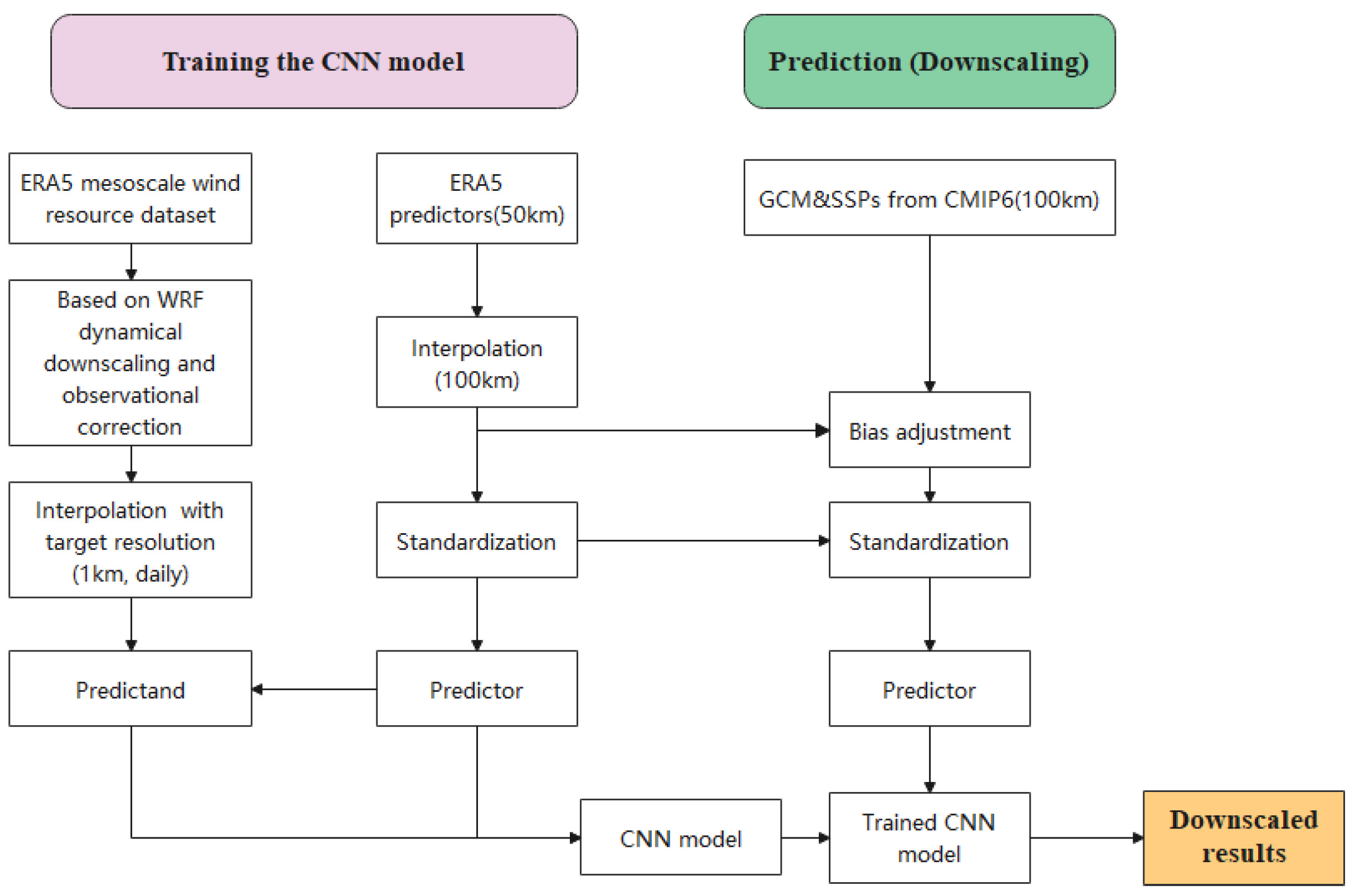
The potential of CNN’s topology lies in its effectiveness in handling complex spatial features. These models can handle high-dimensional predictor variable spaces, automatically selecting variables and geographical regions that influence each site during the downscaling process. This is crucial because modern statistical downscaling methods, such as mature Generalized Linear Models, struggle to handle such high dimensionality without overfitting, often requiring some form of manually guided feature selection (resulting in the loss of relevant information) [28]. This study used high-dimensional input grids and various predictor variables to test the CNN model. Simultaneously, the predictor variables from both the historical period and the observed dataset of surface wind speed for the training of the CNN model are adopted, with a high resolution of 1 km (Figure 3). Subsequently, the predictions of these scenarios using our trained model are downscaled, separately performing downscaled processing for both the historical period (1980–2014) and the SSPs (2015–2100).

2.4. Metrics

The simulated surface wind speed accuracy was assessed by comparing the pixel values (Mi) corresponding to the latitude and longitude of the measurement towers with the observed values (Gi). The several statistical metrics used for validation include four indexes. The Coefficient of Determination (R2) measures the proportion of variance in the observed data (Gi) explained by the simulated data (Mi). A higher R2 value indicates a stronger linear relationship between the two datasets. Mean Bias (MB) represents the average difference between the simulated surface wind speed (Mi) and the observed measured values (Gi). A positive MB value indicates overestimation by the model, while a negative value indicates underestimation. Root Mean Square Error (RMSE) measures the standard deviation of the differences between simulated and observed values (MiGi). A smaller RMSE indicates higher accuracy in the model predictions. Index of Agreement (IOA) indicates the degree of agreement between simulated and observed data, with 1 indicating perfect agreement. A higher IOA value indicates better consistency between the two datasets. The equations for these parameters are as follows:
R 2 = ( i = 1 n ( M i M ¯ ) ( G i G ¯ ) ) 2 i = 1 n ( M i M ¯ ) 2 i = 1 n ( G i G ¯ ) 2 , 0 R 2 1
R M S E = 1 n i = 1 n ( M i G i ) 2
M B = 1 N i = 1 n ( M i G i )
I O A = 1 i = 1 n ( M i G i ) 2 i = 1 n ( | M i G ¯ | + | G i G ¯ | ) 2
The subscript i represents individual samples, and n is the total number of samples used for evaluation. The significance of each parameter contributes to assessing the model’s performance in estimating surface wind speed.

3. Results

3.1. Testing and Validation of the CNN Downscaling Model

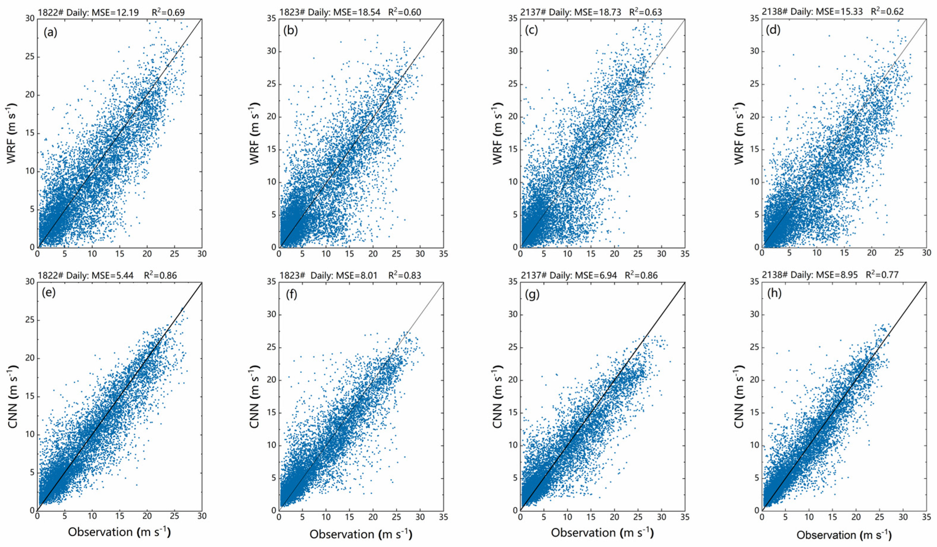
Before employing the CNN downscaling model, it is examined using data from the wind towers (1822#, 1823#, 2137#, and 2138#). As shown in Figure 4, the WRF numerical simulation results strongly correlate with the observed values serving as the training target. The R2 values are above 0.6 (1822#: 0.69, 1823#: 0.60, 2137#: 0.63, 2138#: 0.62), passing the significance test with p < 0.05. From the bottom row of Figure 4, it can be observed that the CNN training model’s test results are almost equivalent to the annual mean bias of the WRF simulation. However, the goodness of fit of the CNN downscaling model test results essentially reaches 0.7 (1822#: 0.86, 1823#: 0.83, 2137#: 0.86, 2138#: 0.77). The downscaling results are comparable to the WRF simulation, and the CNN downscaling simulation results are more stable (MSE < 10 m·s−1). This is because the model also uses the observed values from the wind towers as training targets, so the training results of the CNN model are better than WRF. However, the errors in the WRF simulation results are within an acceptable range and can be used as valid values for training targets. Based on this conclusion, the downscaled wind speeds from the CNN downscaling model for CMIP6 can be used as the basis for subsequent research.
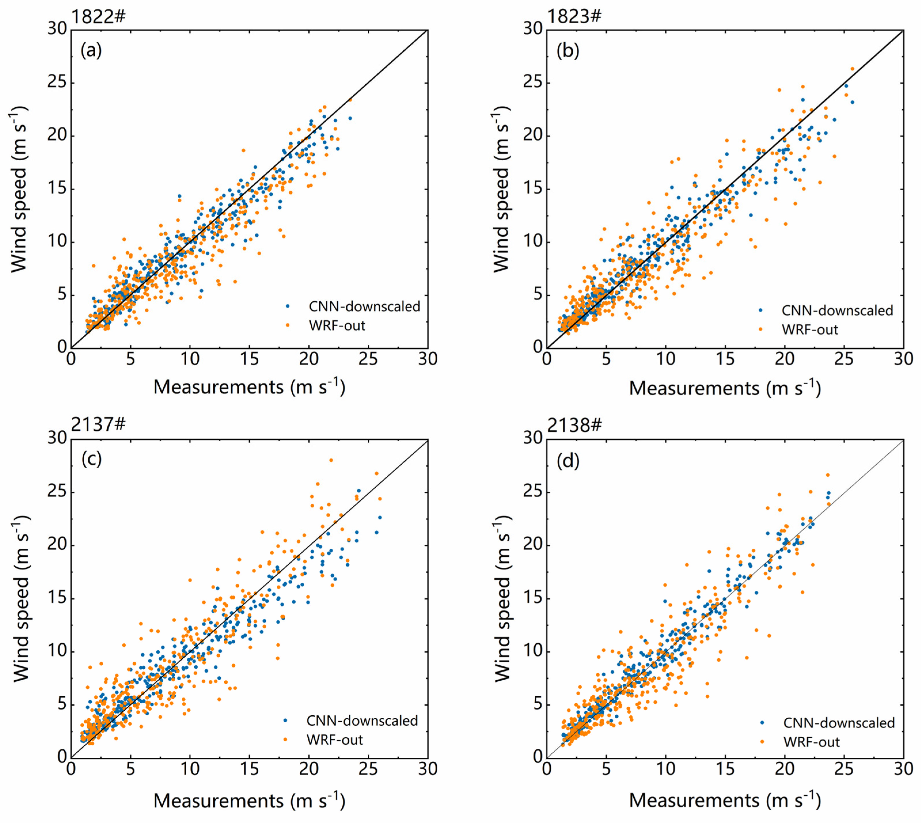
Meanwhile, utilizing the WRF numerical simulation results as the training target, the CNN downscaled model was employed to downscale the wind speed of CMIP6 with the climate dataset as input, downsizing the original data to kilometer-scale, daily-scale wind resource data. Subsequently, an extrapolation parameterization scheme proposed by Touma [29] was applied to extrapolate the results to a hub height of 100 m. At the site scale, Figure 5 presents a time series comparison between the downscaling results and the actual wind tower measurements. The time series comparison graphs illustrate a very high level of consistency between the simulation results of both. Table 2 shows the statistical results of relative errors for independent validation at locations (1822#, 1823#, and 2137#) for both cases. The annual average wind speeds at the wind tower locations (1822#, 1823#, and 2137#) are 6.93 m·s−1, 7.03 m·s−1, and 5.74 m·s−1, respectively. The WRF numerical simulation yields 6.91 m·s−1, 6.82 m·s−1, and 5.85 m·s−1 at these locations. For CMIP6, the downscaled wind speeds in two scenarios are 6.7 m·s−1, 6.96 m·s−1, 5.87 m·s−1, and 6.83 m·s−1, 7.13 m·s−1, 5.92 m·s−1, respectively. The relative errors for WRF and CMIP6 are below 4% compared to the measured wind tower values. The R2 values are higher than 0.6, and the IOA values are higher than 0.8. The differences between the downscaled results for the two scenarios are small. Due to the region’s limited number of wind towers, a simple error analysis indicates that both approaches have stable and consistent technical pathways and implementation schemes, with simulation results below 4% error.

3.2. The Spatial Distribution of CNN Downscaled the CMIP6 Results

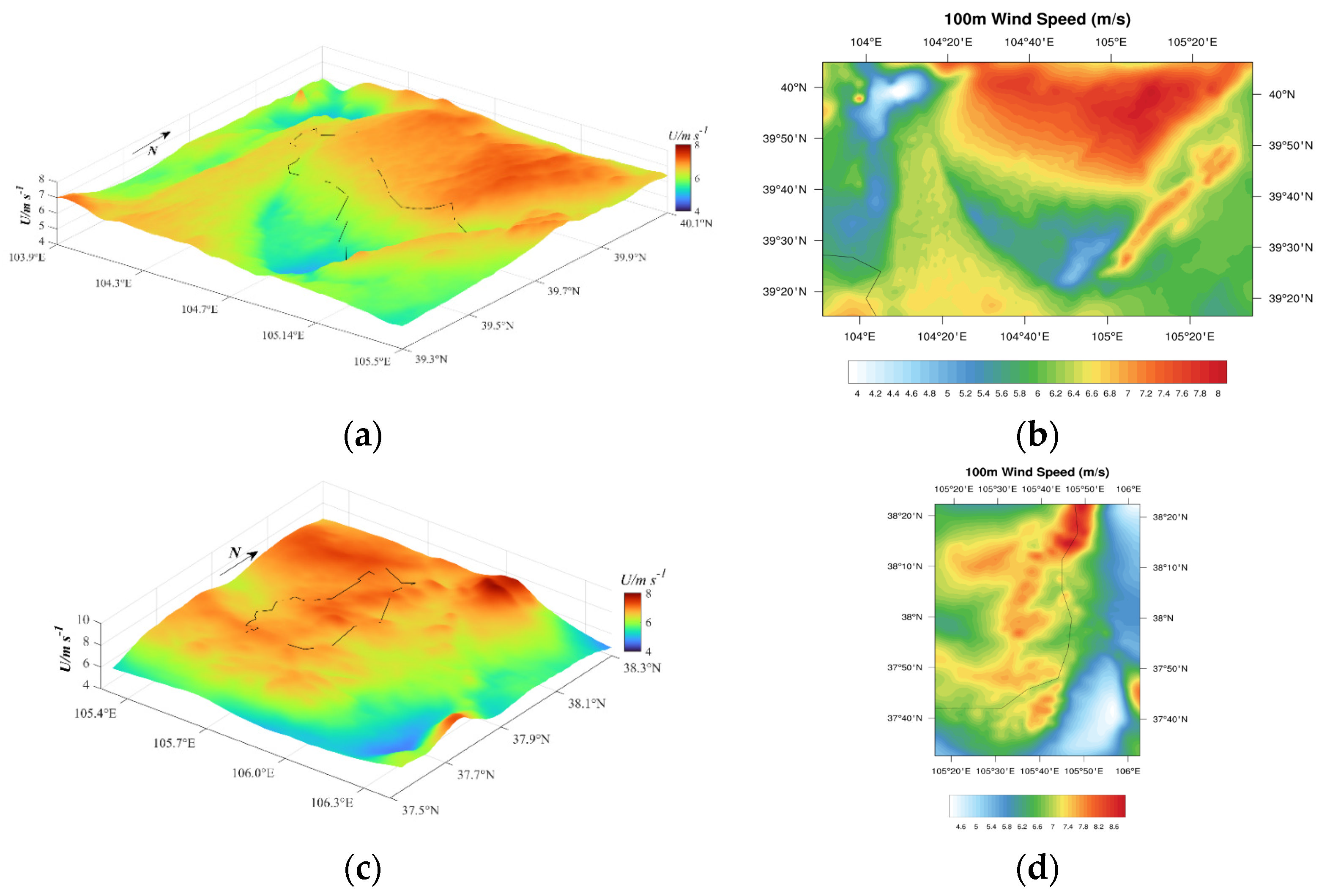
In the preceding section, an analysis of the downscaled results was conducted at the site scale during the measurement period of the wind tower. This section compared the spatial distribution of WRF numerical simulation results and the downscaled results from CMIP6 (ssp245) during the wind tower period. As shown in Figure 6, the spatial distribution maps depict the downscaled results from CMIP6 and the numerical simulation results from WRF in the project area (d03 and d04), respectively. The left figure displays a three-dimensional representation of the WRF numerical simulation results, while the correct figure illustrates the two-dimensional spatial distribution of downscaled wind speeds from CMIP6 (ssp245). The top-left graph reveals the actual wind resource situation in the d03 region, showing a pattern of higher wind resources in the north and lower in the south. This is consistent with the results in the top-right graph, where wind resource distribution is around 7 m·s−1. Additionally, there is a noticeable gradient from northeast to southwest, which is correlated with the region’s topography. The graph below illustrates the actual distribution of wind resources in the d04 region. Both results indicate significant fluctuations in wind resources or uneven distribution of isopleths attributed to the area’s mountainous terrain and complex topography. The wind speed distribution ranges from 7.5 m·s−1 to 8 m·s−1, showing consistency in spatial distribution between the two.
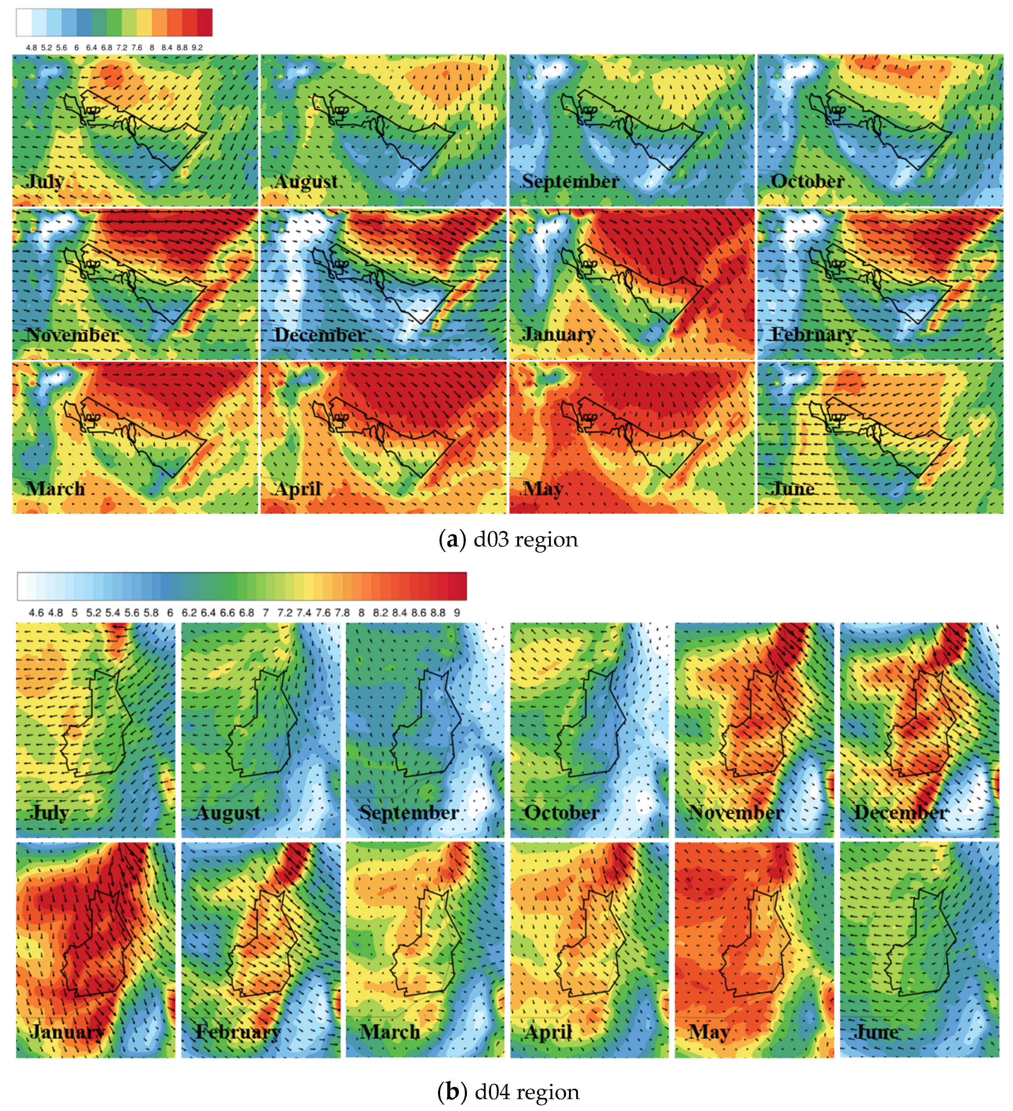
Building upon the above results, the downscaled wind speed results from CMIP6 effectively capture the actual conditions in the experimental area. Subsequently, the downscaling processing on CMIP6 mid-term (2015–2050) climate data is conducted, obtaining spatial distribution maps of multi-year monthly averages. As illustrated in Figure 7, the spatial distribution shown in the upper graph indicates a correlation between wind speed and terrain height in the d03 region. The wind farm exhibits a narrow distribution extending from northwest to southeast, with mountainous areas in the northern and eastern parts. The northern mountains contribute to elevation changes in the topography, with areas at higher altitudes experiencing less resistance, leading to higher wind speeds. Consequently, the wind speeds in the northern region of the wind farm are generally higher. In the eastern region of the wind farm, the canyon terrain between the northern and eastern mountain ranges also enhances wind speeds. Overall, the spatial distribution pattern of wind speed tends to be higher in the north and west and lower in the south and east. By examining the monthly wind speed maps, it can be observed that the wind speeds in the d03 wind farm area are generally higher during the winter and spring seasons (November to May of the following year), dominated by westerly winds. It is attributed to the influence of large-scale westerly circulation during the winter, making it a primary period for wind power generation. The wind speed maps provide a more intuitive visualization of the trend in wind speed variations across the entire d03 wind farm area. By examining the monthly wind speed maps, it becomes evident that the wind speeds in the d04 wind farm are generally higher during the winter and spring seasons (November to May of the following year), highlighting these periods as crucial for wind power generation. Simultaneously, the wind speed maps and the topographical height map of d04 visually represent the wind speed distribution across the entire d04 wind farm area. In the d04 wind farm area, northwest winds prevail. In the western part of the area, there are residual ranges of the Helan Mountains with higher elevation and less resistance, resulting in higher wind speeds [30]. The high wind speed zones are also primarily distributed near the ridges. The overall topography of the area exhibits a trend of higher elevation in the west and lower elevation in the east, resulting in a pattern of higher wind speeds in the west and lower in the east.

3.3. Future Mid-Term (2015–2050) Wind Speed Variations

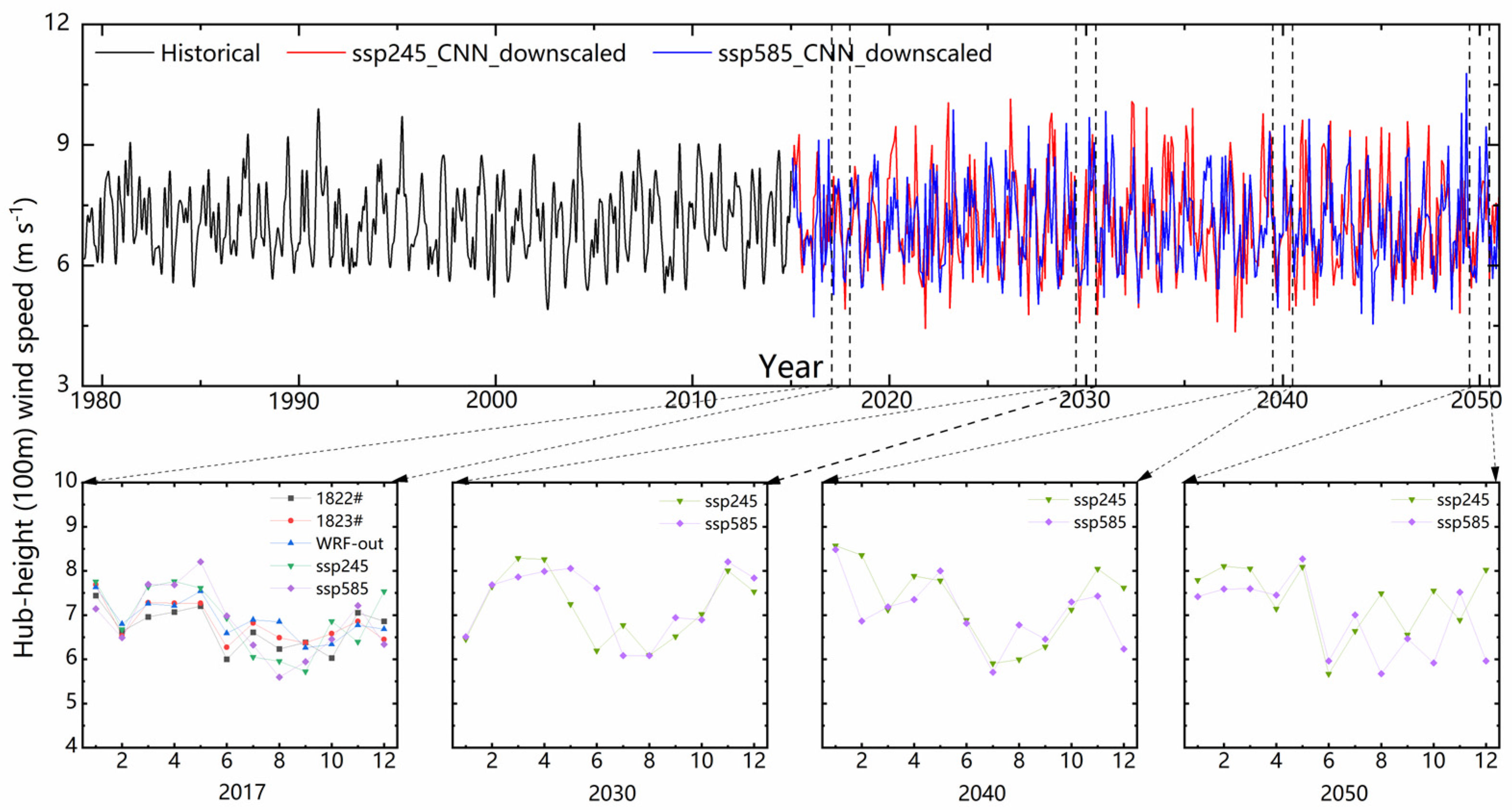
Based on the downscaled wind speed climate data from CMIP6, as discussed above, the trend of future mid-term wind speed variations is analyzed in the wind farm area over time. Figure 8 illustrates the monthly scale time series of wind speed variations in the d03 region for historical and future mid-term periods. It can be observed that the wind speed changes are subtle in both scenarios, with future average wind speeds of 7.06 m·s−1 and 7.00 m·s−1, respectively. These values are consistent with the historical wind speed of 7.10 m·s−1. Furthermore, the downscaled results, wind tower data, and WRF numerical simulation results are compared during the measurement period of the wind tower. The research results reveal that all results exhibit consistent variations throughout the year. In the future periods of 2030, 2040, and 2050, a similar analysis of the annual wind speed variations is conducted. The more significant fluctuations are observed compared to 2017, with high wind speeds occurring predominantly in winter and spring.
In summary, considering the wind energy distribution, the prevailing wind direction in the wind farm area is predominantly WNW. The overall wind speed distribution is extensive, aligning with the requirements for wind farm construction. When planning the layout of wind turbines, it is advisable to consider arranging them along ridges, as this is conducive to the development of the wind farm.

4. Conclusions

Based on wind data and reanalysis information, analyzing the historical climate characteristics of wind energy can provide references for wind farm site selection and short-term power generation forecasts. In the vast wind power bases in the deserts, Gobi, and barren areas of northern China, research on the future characteristics of wind energy resources is often relatively scarce due to limited wind measurement data. This scarcity leads to significant uncertainty challenges in assessing wind farms’ long-term power generation profitability. This study focuses on a wind farm in the Tengger Desert as the research area. Using a constructed DL downscaling algorithm, the CMIP6 wind speed data are downscaled to analyze and compare wind energy’s past and future characteristics. The research results indicate:
(1)
The DL downscaling algorithm applied to CMIP6 wind speed data provides reliable results, demonstrating its effectiveness in capturing wind energy’s spatial and temporal characteristics in the study area. Validation using data from three effective wind towers indicates that the annual average wind speed errors are all below 4%.
(2)
The spatial distribution of wind speed variations is influenced by the topography, with higher wind speeds observed in areas of lower elevation and less resistance, such as in the northern and western parts of the wind farm area.
(3)
The future mid-term wind speed variations in the study area show subtle changes, with average wind speeds consistent with historical values. This stability is crucial for assessing wind power generation’s long-term profitability and reliability.
In conclusion, this study contributes valuable insights into the historical and future characteristics of wind energy in the Tengger Desert region, providing a foundation for a better understanding of wind resources and aiding in the sustainable development of wind power in northern China.
Despite the downscaling model proposed in this study has demonstrated certain effectiveness, it still has certain limitations. Firstly, the data used in this research may be subject to constraints, such as spatiotemporal resolution, quality, and availability. This could potentially impact the accuracy and comprehensiveness of the study. Secondly, the models employed in this research may be based on certain assumptions that may be valid in specific contexts but may not be applicable in other situations. This could influence the predictions and reliability of the models. Additionally, as the research primarily focuses on the Tengger Desert region, the findings may lack universality and cannot be directly extrapolated to other geographical areas. Variances in geography, climate, and environmental conditions may result in different wind energy characteristics. Lastly, the DL models developed in this study may be optimized for specific conditions, and their performance in different environments may not meet expectations.

Author Contributions

H.Z. and Q.L. led the writing of this paper and acknowledge responsibility for the experimental data and results. H.Z. and L.Y. drafted the paper, and Q.L. led the consolidation of the input and simulation dataset. This paper was written in cooperation with all of the co-authors. All authors have read and agreed to the published version of the manuscript.

Funding

This research was funded by the Research and Application of Future Medium to Long-Term Wind Resource Assessment for Wind Farms Based on Artificial Intelligence Project, grant number 2023021. The article publishing charge (APC) was funded by the Economic Transformation of Climate Resources Key Laboratory of the China Meteorological Administration and Chongqing Shete Meteorological Application Research Institute.

Institutional Review Board Statement

Not applicable.

Informed Consent Statement

Not applicable.

Data Availability Statement

Data are contained within the article.

Acknowledgments

We are grateful for the datasets provided by the European Centre for Medium-Range Weather Forecasts (ECWMF), https://www.ecmwf.int/ (accessed on 7 January 2024). The Coupled Model Intercomparison Project Phase 6 (CMIP6), https://esgf-node.llnl.gov/projects/cmip6/ (accessed on 7 January 2024). The Measurements of the Wind Tower from Haizhuang Wind Power Co., Ltd., China State Shipbuilding Corp (CSSC), https://www.cssc-hz.com/?en/ (accessed on 7 January 2024). The authors would like to thank all their colleagues at the observation stations on the TP for their maintenance of the instruments.

Conflicts of Interest

The authors declare that they have no known competing financial interests or personal relationships that could have appeared to influence the work reported in this paper. Ling Yuan is employee of Haizhuang Wind Power Co., Ltd. The paper reflects the views of the scientists, and not the company.

References

  1. de Castro, M.; Salvador, S.; Gómez-Gesteira, M.; Costoya, X.; Carvalho, D.; Sanz-Larruga, F.J.; Gimeno, L. Europe, China, and the United States: Three different approaches to the development of offshore wind energy. Renew. Sustain. Energy Rev. 2019, 109, 55–70. [Google Scholar] [CrossRef]
  2. Tian, Q.; Huang, G.; Hu, K.; Niyogi, D. Observed global climate model-based changes in wind power potential over the Northern Hemisphere during 1979–2016. Energy 2019, 167, 1224–1235. [Google Scholar] [CrossRef]
  3. Vautard, R.; Cattiaux, J.; You, P.; Thépaut, J.N.; Ciais, P. Northern Hemisphere atmospheric stilling is partly attributed to an increase in surface roughness. Nat. Geosci. 2010, 3, 756–761. [Google Scholar] [CrossRef]
  4. McVicar, T.R.; Roderick, M.L.; Donohue, R.J.; Li, L.T.; Van Niel, T.G.; Thomas, A.; Grieser, J.; Jhajharia, D.; Himri, Y.; Mahowald, N.M.; et al. Global review and synthesis of trends in observed terrestrial near-surface wind speeds: Implications for evaporation. J. Hydrol. 2012, 416, 182–205. [Google Scholar] [CrossRef]
  5. Pryor, S.C.; Barthelmie, R.J.; Young, D.T.; Takle, E.S.; Arritt, R.W.; Flory, D.; Roads, J. Wind speed trends over the contiguous United States. J. Geophys. Res. Atmos. 2009, 114, D14015. [Google Scholar] [CrossRef]
  6. Chen, L.; Li, D.; Pryor, S.C. Wind speed trends over China: Quantifying the magnitude and assessing causality. Int. J. Climatol. 2013, 33, 2579–2590. [Google Scholar] [CrossRef]
  7. Fant, C.; Schlosser, C.A.; Strzepek, K. The impact of climate change on wind and solar resources in southern Africa. Appl. Energy 2016, 161, 556–564. [Google Scholar] [CrossRef]
  8. Meehl, G.A.; Boer, G.J.; Covey, C.; Latif, M.; Stouffer, R.J. Intercomparison makes for a better climate model. Eos 1997, 78, 445–451. [Google Scholar] [CrossRef]
  9. Eyring, V.; Bony, S.; Meehl, G.A.; Senior, C.A.; Stevens, B.; Stouffer, R.J.; Taylor, K.E. Overview of the Coupled Model Intercomparison Project Phase 6 (CMIP6) experimental design and organization. Geosci. Model Dev. 2016, 9, 1937–1958. [Google Scholar] [CrossRef]
  10. Stott, P.A.; Mitchell JF, B.; Allen, M.R.; Delworth, T.L.; Gregory, J.M.; Meehl, G.A.; Santer, B.D. Observational constraints on past attributable warming and predictions of future global warming. J. Clim. 2006, 19, 3055–3069. [Google Scholar] [CrossRef]
  11. Lee, J.Y.; Wang, B. Future change of global monsoon in the CMIP5. Clim. Dyn. 2014, 42, 101–119. [Google Scholar] [CrossRef]
  12. Zheng, C.; Li, X.; Luo, X.; Chen, X.; Qian, Y.; Zhang, Z.; Chen, Y. Projection of Future Global Offshore Wind Energy Resources using CMIP Data. Atmos. Ocean 2019, 57, 134–148. [Google Scholar] [CrossRef]
  13. Pryor, S.C.; Barthelmie, R.J. Assessing climate change impacts on the near-term stability of the wind energy resource over the United States. Proc. Natl. Acad. Sci. USA 2011, 108, 8167–8171. [Google Scholar] [CrossRef]
  14. Kulkarni, S.; Deo, M.C.; Ghosh, S. Framework for assessment of climate change impact on offshore wind energy. Meteorol. Appl. 2018, 25, 94–104. [Google Scholar] [CrossRef]
  15. Zhou, T.; Chen, Z.; Zou, L.; Chen, X.; Yu, Y.; Wang, B.; Bao, Q.; Bao, Y.; Cao, J.; He, B.; et al. Development of Climate and Earth System Models in China: Past Achievements and New CMIP6 Results. J. Meteorol. Res. 2020, 34, 1–19. [Google Scholar] [CrossRef]
  16. Maraun, D.; Widmann, M. Statistical Downscaling and Bias Correction for Climate Research; Cambridge University Press: Cambridge, UK, 2018. [Google Scholar]
  17. Kotlarski, S.; Keuler, K.; Christensen, O.B.; Colette, A.; Déqué, M.; Gobiet, A.; Goergen, K.; Jacob, D.; Lüthi, D.; van Meijgaard, E.; et al. Regional climate modeling on European scales: A joint standard evaluation of the EURO-CORDEX RCM ensemble. Geosci. Model Dev. 2014, 7, 1297–1333. [Google Scholar] [CrossRef]
  18. Harris, L.; McRae, A.T.; Chantry, M.; Dueben, P.D.; Palmer, T.N. A generative deep learning approach to stochastic downscaling of precipitation forecasts. J. Adv. Model. Earth Syst. 2022, 14, e2022MS003120. [Google Scholar] [CrossRef] [PubMed]
  19. Leinonen, J.; Nerini, D.; Berne, A. Stochastic super-resolution for downscaling time-evolving atmospheric fields with a generative adversarial network. IEEE Trans. Geosci. Remote Sens. 2020, 59, 7211–7223. [Google Scholar] [CrossRef]
  20. Thrasher, B.; Xiong, J.; Wang, W.; Melton, F.; Michaelis, A.; Nemani, R. Downscaled climate projections suitable for resource management. Eos Trans. Am. Geophys. Union 2013, 94, 321–323. [Google Scholar] [CrossRef]
  21. Trzaska, S.; Schnarr, E. A Review of Downscaling Methods for Climate Change Projections; United States Agency for International Development by Tetra Tech ARD: Washington, DC, USA, 2014; pp. 1–42. [Google Scholar]
  22. Wilby, R.L.; Dawson, C.W. The statistical downscaling model: Insights from one decade of application. Int. J. Climatol. 2013, 33, 1707–1719. [Google Scholar] [CrossRef]
  23. Reichstein, M.; Camps-Valls, G.; Stevens, B.; Jung, M.; Denzler, J.; Carvalhais, N.; Prabhat, F. Deep learning and process understanding for data-driven Earth system science. Nature 2019, 566, 195–204. [Google Scholar] [CrossRef]
  24. Schmidhuber, J. Deep Learning in neural networks: An overview. Neural Netw. 2015, 61, 85–117. [Google Scholar] [CrossRef]
  25. Yamashita, R.; Nishio, M.; Do RK, G.; Togashi, K. Convolutional Neural Networks: An Overview and Application in Radiology—Insights into Imaging; Springer: Berlin/Heidelberg, Germany, 2018. [Google Scholar]
  26. Ahmed, S.F.; Alam MS, B.; Hassan, M.; Rozbu, M.R.; Ishtiak, T.; Rafa, N.; Gandomi, A.H. Deep learning modeling techniques: Progress, applications, advantages, and challenges. Artif. Intell. Rev. 2023, 56, 13521–13617. [Google Scholar] [CrossRef]
  27. Bazgir, O.; Zhang, R.; Dhruba, S.R.; Rahman, R.; Ghosh, S.; Pal, R. Representation of features as images with neighborhood dependencies for compatibility with convolutional neural networks. Nat. Commun. 2020, 11, 4391. [Google Scholar] [CrossRef]
  28. Kheir AM, S.; Elnashar, A.; Mosad, A.; Govind, A. An improved deep learning procedure for statistical downscaling of climate data. Heliyon 2023, 9, e18200. [Google Scholar] [CrossRef] [PubMed]
  29. Touma, J.S. Dependence of the wind profile power law on stability for various locations. J. Air Pollut. Control Assoc. 1977, 27, 863–866. [Google Scholar] [CrossRef]
  30. Han, F.; Li, H.; Zhu, M.; Zhang, R.; Zhou, W. Application of a meso-microscale coupled modeling method to wind resource assessment. Energy Eng. 2023, 43, 32–40. [Google Scholar]
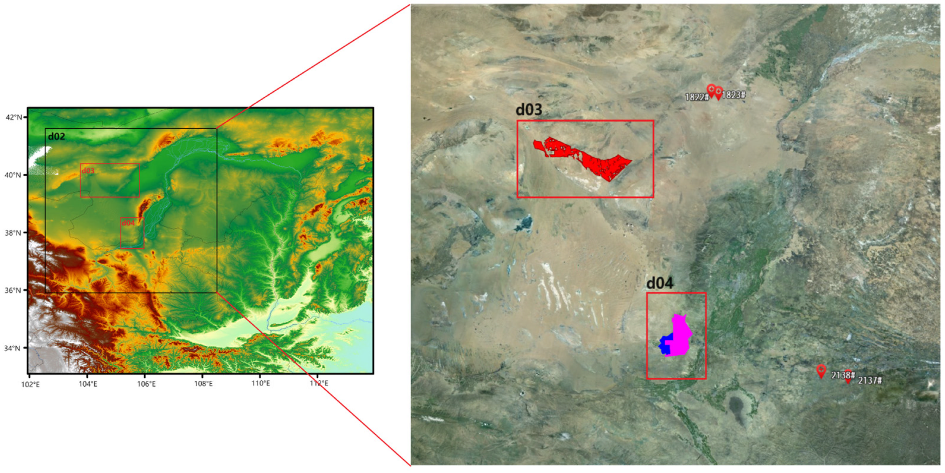
Figure 1. Topography map of the wind farms in the study area. The left panel illustrates the spatial distribution of elevations in the study area, with red indicating higher elevations and green indicating lower elevations. The right panel highlights the d03 region within the red border, while the blue and purple borders represent the d04 region. Pointers indicate the geographical locations of the measurement towers.
Atmosphere 15 00271 g001
Figure 2. Technical scheme for downscaling ERA5 near-surface wind speed based on the convolutional neural network (CNN) algorithm.
Atmosphere 15 00271 g002
Figure 3. Workflow and steps of the preprocessing method for downscaling CMIP6 scenarios using the convolutional neural network (CNN) algorithm. Purple sections represent the training, testing, and validation stages during the CNN downscaling model generation. Green sections indicate the application stage of the model. Yellow section represents the output results of the model.
Atmosphere 15 00271 g003
Figure 4. Regression correlation statistics between observed values (Observations) and WRF simulation (WRF-out) results (ad) and CNN downscaled simulation predictions (CNN) based on ERA5 Reanalysis data (eh) during 2017–2018 at four wind towers (1822#, 1823#, 2137# and 2138#).
Atmosphere 15 00271 g004
Figure 5. Time series comparison of 100 m wind speeds between the wind tower measurements ((a) 1822#, (b) 1823#, (c) 2137#, and (d) 2138#) from 2017 to 2018 (Measurements) and CMIP6 (ssp245) downscaled results (CNN-downscaled) (blue dots) and WRF simulation results (WRF-out) (yellow dots).
Atmosphere 15 00271 g005
Figure 6. Comparison of the spatial distribution between WRF numerical simulation results (a,c) and CMIP6 (ssp245) downscaled results (b,d) in the project area (d03 and d04).
Atmosphere 15 00271 g006
Figure 7. Spatial distribution of multi-year monthly average results of downscaled wind speed climate data from CMIP6 (ssp245) for the mid-term period (2015–2050) in the project area (d03 and d04). The black arrow represents the flow field diagram. The black solid lines represent the project scope boundaries of d03 and d04, respectively.
Atmosphere 15 00271 g007
Figure 8. Time-series analysis of historical monthly wind speed (1978–2014), future mid-term (2015–2050) monthly wind speed variations of CMIP6 downscaled results (ssp245 and ssp585), and wind tower measurements at1822# and 1823# in the study area (d03 region).
Atmosphere 15 00271 g008
Table 2. Error statistics for validating 100 m wind speeds downscaled from WRF simulation results (WRF-out) and CMIP6 (ssp245 and ssp585) based on wind tower measurements (1822#, 1823#,2137# and 2138#).
Wind Speed of Measurements (m·s−1)WRF-Out Wind Speed (m·s−1)CMIP6 (ssp245/ssp585)
Wind Speed (m·s−1)RMSE (m·s−1)MB (m·s−1)BIAS (%)R2IOA
1822#6.936.916.70/6.832.16/2.02−0.23/−0.13.32%/1.44%0.61/0.660.81/0.80
1823#7.036.826.96/7.132.07/2.36−0.07/0.10.99%/1.42%0.64/0.620.87/0.85
2137#5.745.855.87/5.921.49/1.980.13/0.182.26%/3.34%0.60/0.610.84/0.82
2138#5.645.515.82/5.791.36/1.68−0.11/0.161.89%/2.76%0.67/0.620.86/0.84
Disclaimer/Publisher’s Note: The statements, opinions and data contained in all publications are solely those of the individual author(s) and contributor(s) and not of MDPI and/or the editor(s). MDPI and/or the editor(s) disclaim responsibility for any injury to people or property resulting from any ideas, methods, instructions or products referred to in the content.