Article

Improving Solar Radiation Prediction in China: A Stacking Model Approach with Categorical Boosting Feature Selection

1
College of Horticulture and Plant Protection, Henan University of Science and Technology, Luoyang 471000, China
2
School of Energy Science and Engineering, Harbin Institute of Technology, 92, West Dazhi Street, Harbin 150001, China
3
College of Agricultural Equipment Engineering, Henan University of Science and Technology, Luoyang 471000, China
4
Key Laboratory for Agricultural Soil and Water Engineering in Arid Area of Ministry of Education, Northwest A&F University, Xianyang 712100, China
*
Authors to whom correspondence should be addressed.
Atmosphere 2024, 15(12), 1436; https://doi.org/10.3390/atmos15121436
Submission received: 30 October 2024 / Revised: 26 November 2024 / Accepted: 28 November 2024 / Published: 29 November 2024
(This article belongs to the Section Atmospheric Techniques, Instruments, and Modeling)

Abstract

:
Solar radiation is an important energy source, and accurately predicting it [daily global and diffuse solar radiation (Rs and Rd)] is essential for research on surface energy exchange, hydrologic systems, and agricultural production. However, Rs and Rd estimation relies on meteorological data and related model parameters, which leads to inaccuracy in some regions. To improve the estimation accuracy and generalization ability of the Rs and Rd models, 17 representative radiation stations in China were selected. The categorical boosting (CatBoost) feature selection algorithm was utilized to construct a novel stacking model from sample and parameter diversity perspectives. The results revealed that the characteristics related to sunshine duration (n) and ozone (O3) significantly affect solar radiation prediction. The proposed new ensemble model framework had better accuracy than base models in root mean square error (RMSE), coefficient of determination (R2), mean absolute error (MAE), and global performance index (GPI). The solar radiation prediction model is more applicable to coastal areas, such as Shanghai and Guangzhou, than to inland regions of China. The range and mean of RMSE, MAE, and R2 for Rs prediction are 1.5737–3.7482 (1.9318), 1.1773–2.6814 (1.4336), and 0.7597–0.9655 (0.9226), respectively; for Rd prediction, they are 1.2589–2.9038 (1.8201), 0.9811–2.1024 (1.3493), and 0.5153–0.9217 (0.7248), respectively. The results of this study can provide a reference for Rs and Rd estimation and related applications in China.

Graphical Abstract

1. Introduction

Solar radiation is an important energy source for all activities on Earth [1,2]. It is critical for exchanging energy on the Earth’s surface and influences weather and climate [3,4]. Daily global and diffuse solar radiation (Rs and Rd) are vital metrics for assessing solar radiation and are critical in designing and optimizing solar energy systems [5,6,7].
As a result of the high cost of installing and maintaining solar radiation instruments [8,9], obtaining reliable Rs and Rd data is difficult [10], and only a few meteorological stations worldwide record solar radiation data [11,12]. Therefore, scholars have proposed various methods to generate high-quality Rs and Rd data [13,14], such as by using empirical and machine learning (ML) models [15]. Common empirical models utilize n and temperature data to build estimation models [16]. For example, Bailek et al. [17] tested the monthly scattering radiation performance of 35 empirical models based on temperature and n in the Sahara region. The results demonstrated that the quadratic equation model proposed for surface applications is the most accurate. Souza et al. [18] predicted solar radiation in Brazil using the Ångström–Prescott empirical model and utilizing sunshine-hour data. They recommended the use of this model in areas where data on n are available. By comparing empirical models that utilize n, temperature, and other meteorological data, Uçkan et al. [19] determined that the model considering other meteorological factors has higher accuracy and is globally applicable. However, when using the empirical model, reflecting the nonlinear and multidimensional relationship between solar radiation and input features in noisy environments is difficult [20]. Compared with the empirical model, the ML model is more accurate and can better solve nonlinear problems [21]. Accordingly, it has been widely utilized in predicting solar radiation. Muhammed et al. [22] proposed using MLP, ANFIS, and SVM algorithms to predict solar radiation in Cairo, Egypt. The results revealed that the MLP model significantly improves solar radiation prediction. Feng et al. [23] compared the daily global solar radiation predictions of four ML models and four temperature-based empirical models in China. The results reveal that the hybrid mind evolutionary algorithm and ANN model are more accurate than existing ML and empirical models. Although ML algorithms yield more accurate prediction results, they also suffer from the limitation in single-model learning performance caused by randomness, which leads to poor generalization ability of the model. Considering the limitations of a single model, scholars often use an integrated model to predict solar radiation [24]. Dong et al. [25] evaluated the potential of three ML algorithms [support vector machine regression (SVR), Extreme Gradient Boosting (XGBoost), and multivariate adaptive regression splines (MARS)] for estimating Rd using conventional meteorological data from five Chinese weather stations as input. The ensemble learning algorithm demonstrated superior performance and stability. Lee et al. proposed four solar radiation prediction models based on ensemble learning (boosted trees, bagged trees, random forest, and generalized random forest) and compared them with SVR and Gaussian process regression. The results revealed that the ensemble learning method performs well [26]. Additionally, the accuracy of the ensemble learning algorithm surpasses that of a single model, which is achieved by building multiple homogeneous or heterogeneous learning models into an ensemble model [27,28]. However, among the three ensemble learning strategies (bagging, boosting, and stacking), only the stacking model can combine different learners. Moreover, it has low data requirements [29]. By integrating the results of varying base learners, the variance can be reduced and the stability of the model can be improved [30].
Temperature and n are widely modeled to predict radiation because of their representativeness [23]. In addition, other environmental factors and geographic information, such as relative humidity, precipitation, longitude, and latitude, are considered [31]. Radiation decay has recently been a trend in many parts of the world, primarily due to increasing atmospheric pollution [32,33]. For instance, particulate matter (PM2.5 and PM10), carbon monoxide (CO), nitrogen dioxide (NO2), sulfur dioxide (SO2), and O3 cause radiation attenuation by scattering and absorbing solar radiation [34]. Moreover, conventional meteorological factors may not be good predictors of solar radiation. Accordingly, the predictive influence of air pollutants on solar radiation has attracted the attention of many scholars in recent years [35]. Sun et al. [36] established different RF models by considering the impact of the air pollution index. They found that introducing air pollution data as input can improve RF performance, and the RMSE values could be reduced by 2.0–17.4%. Increasing the number of variables often triggers information redundancy and dimensional catastrophe, thus reducing the performance of the building models [37]. To boost the estimation accuracy of ML, it is important to select model input factors appropriately [38]. For example, using three feature selection methods (recursive feature elimination, variable selection using random forests, and least absolute shrinkage and selection operator (LASSO)), Luo et al. developed a model for the estimation of forest biomass based on various features [39]. The utility of ML models is evinced in the transparency of the model, that is, the effect of input features on the ability to make predictions. When performing tests using black box models, potential errors inherited from training data may lead to significant biases in the results, thus diminishing the confidence in complex black box models [40]. Although many global model interpretation methods exist, such as decision tree-based models that output the mean importance of features, they cannot characterize the effect of individual features on the sample. Therefore, methods for achieving local model interpretation have recently been proposed, such as local interpretable model agnostic explanation [41] and Shapley additive explanations (SHAPs) [42]. For example, Ding et al. [43] used SHAP to determine the key parameters affecting the maturity prediction of compost, and Mitrentsis et al. [40] interpreted PV prediction models by calculating SHAP.
This study aims to build predictive and transparent ML models to improve the accuracy of predicting solar radiation and the interpretability of the models. There were 17 regions selected from different climatic zones in China, and the CatBoost feature selection algorithm was used to output the importance of each feature to determine the input combinations of the model at different stations. Five ML models with low correlation and good performance were selected to construct the stacking model framework. The SHAP values were used to explain the influence of different features on the construction of the stacking model and to evaluate the applicability of the model in China. Although many scholars have employed ML models to predict solar radiation, to the best of our knowledge, no one has combined the CatBoost feature selection algorithm and SHAP values to construct a novel solar radiation prediction model. This approach offers significant advantages in terms of predictive performance and interpretability, thereby making valuable contributions to the research and application of solar energy forecasting.

2. Materials and Methods

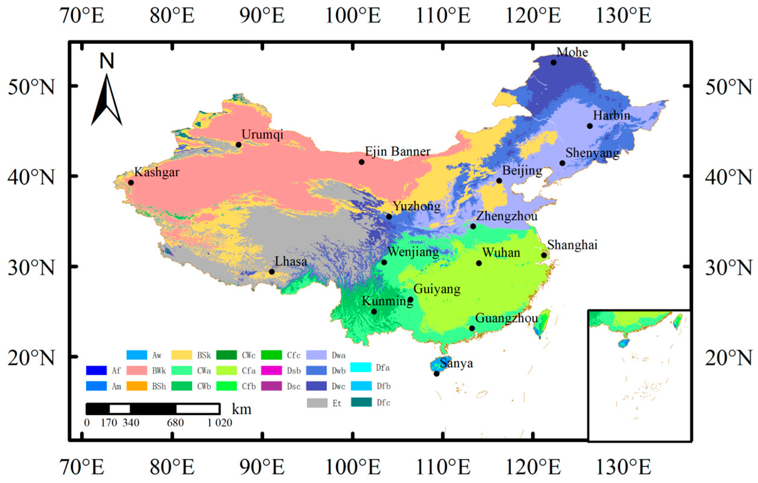
2.1. Data Collection and Processing

The following data were collected from 2015 to 2020 from 17 representative regions in China (Figure 1, Table 1): Rs, Rd, n, mean temperature (Tmean), maximum temperature (Tmax), minimum temperature (Tmin), air pressure (Pr), relative humidity (Rh), precipitation (Pt), wind speed (Ws), and major air pollutant mass concentrations (PM2.5, PM10, CO, SO2, NO2, and O3) as well as the calculated air quality index (AQI). Meteorological and radiation data were obtained from the China Meteorological Data Network accessed on 11 January 2023 (https://data.cma.cn/, accessed on 1 October 2024). Air pollutant data were derived from the China National Environmental Monitoring Center (http://www.cnemc.cn/, accessed on 1 October 2024). In addition, the values of extra-terrestrial solar radiation (Ra), maximum sunshine duration (N), and vapor pressure deficit (Vpd) were determined according to the methods described by Allen et al. [44]. Some incomplete abnormal data were removed from the data set. Notably, Rd/Rs, Rs/Ra, and n/N were greater than 1 [45].

2.2. Evaluation of Model Input Characteristics

2.2.1. CatBoost Feature Selection Algorithm

Feature selection—the removal of redundant variables to improve the model generalization ability and reduce the complexity of the model—is primarily applied in ML. The tree model CatBoost is selected for feature selection in this study to calculate the feature importance. The feature threshold was set manually in previous studies, and because the threshold is primarily determined by the user, irrational problems may arise. To solve this problem, we propose first arranging the feature importance from high to low, obtaining the median of the feature, and then taking the median as the threshold to remove redundant features. CatBoost replaces the traditional gradient boosting algorithm with orderly lifting and permutation driving to reduce the deviation of gradient estimation and enhance the generalization ability. As an ensemble algorithm with a decision tree as the basic learner, the CatBoost expression [46] is as follows:
G N = n = 1 N g n
where G N is the strong ensemble learner and g n is a decision tree based on the residuals of the previous tree.
The use of predictions from the previous tree to train the next tree in CatBoost provides a unique method of calculating feature importance. CatBoost provides a variety of important metrics for assessing the importance of features in the parent features. The change in the predicted value and the transformation of the loss function describe the mean change in the predicted value when the eigenvalue is changed alongside a change in the loss function with or without this feature in the model. The greater the mean change in the predicted value (PVC) or the more significant the change in the loss function (LFC), the more important this feature is.
P V C F = t r e e s , l e a f s F ν 1 α ν r 2 l e a f l + ν 2 α ν r 2 l e a f r
a ν r = ν 1 l e a f l + ν 2 l e a f r l e a f l + l e a f r
L F C j = l e x i l f e a t u r e s
where l e a f 1 and l e a f 2 represent the weights of the left and right lobes, respectively. v 1 and v 2 represent the objective function values of the left and right leaves, respectively. l e x i and l f e a t u r e s represent the loss function value of the model when the model lacks features and the loss function value of the model when all features are used, respectively.

2.2.2. Shapley Additive Explanation

The SHAP implementation in this study is based on the KernelExplainer principle, and weighted linear regression is used to approximate the SHAP value of any model. The SHAP value technique is a model interpretation analysis method based on game theory and local interpretation, which can reflect the influence of features in each sample on the output. In this study, the mean value of the marginal contribution of the feature to the model output in the case of different feature sequences is calculated via the SHAP value technique to generate the SHAP reference value, which obeys the following formula [47]:
y i = y b a s e + f x i 1 + f x i 2 + . . . + f x i j
Suppose that x i j is the jth feature of the ith sample, the baseline of the whole model is y b a s e , and the predicted value of the model for the sample is   y i . Then, f( x i j ) is the SHAP value of x i j , and f( x i j ) > 0 denotes that the feature is positively correlated with the output; otherwise, the feature is negatively correlated with the output.

2.3. Learner Selection for Stacking

In stacking ensemble learning, the selection of learners is essential: the basic learners should choose models with stable performance to improve the overall performance of the model, and maximal differences among learners during learner selection should be ensured. This is necessary because different models essentially use different data spaces and data structures by observing data and building the corresponding models afterward. Additionally, this process is dependent on the principles underlying the algorithms themselves. Therefore, selecting learners that differ considerably can ensure that the advantages of different algorithms are leveraged and each differentiated model learns the benefits of other models. In this study, the Pearson correlation coefficient [48] is used to calculate the difference degree for each model to select the model with a large difference degree. Figure 2 shows that the correlations of the algorithms are generally high due to the high learning ability of the different algorithms. The linear model-based models (linear, ridge, and Bayesian) have the highest correlation, followed by the tree-based ensemble algorithms (RF, XGBoost, GBDT, LightGBM, and CatBoost), mainly because of the apparent similarity in the data observation methods for the same class of algorithms and the low correlation of the different principle models, which is attributable to the training mechanisms of the models with other principles also being very different. Considering the algorithm performance and relevance, we chose the Bayesian model in the linear approach, XGBoost in the ensemble approach, and three other approaches with different operational principles (SVR, ANN, and KNN) as the base learner. A meta-learner mainly considers the generalization ability of the model and robustness to overfitting and generally chooses a relatively simple linear model. In contrast, elastic network regression constrains the coefficients by introducing L1 and L2 regularizations, which can screen the base learner and assign the learner different weights according to the coefficient, which helps improve the generalization ability of the model and combine the advantages of multiple models. The learner principle for building the stacking model is presented in the following sections.

2.3.1. Support Vector Regression (SVR)

SVR is a novel and effective model for dealing with regression problems that have become popular in the world in recent years, which can improve the generalization ability of ML and reduce the problem of overfitting by finding the minimum structural risk, which was rapidly developed [49]. SVR separates samples with different labels by searching for a divided hyperplane in the training set. Only one class of sample points exists in SVR, and the optimal hyperplane minimizes the total deviation between all sample points and the hyperplane. The SVR model in this study utilizes the linear function as a kernel function.

2.3.2. Artificial Neural Networks (ANNs)

ANNs are models composed of many interconnected neurons and are widely used in the analysis of various complex problems [50]. In addition to output and input layers, multiple hidden layers exist in the model [51]. However, simple ANNs only have one hidden layer. Specifically, it has a three-layer structure. In this study, each layer is fully connected by a neuron with a rectified linear unit activation function, and the weighted sum of the output value of each layer is the input of each layer. Detailed computation procedures and information on ANNs are found in the work of Xin [52].

2.3.3. K-Nearest Neighbor (KNN)

The main concept behind the KNN, a simple regression method, is calculating the distance of the unknown sample based on that of the known sample, selecting the k-nearest neighboring samples from the feature space of the known sample, determining the weight generated by distance from the k-neighboring samples to the sample, and calculating the weighted mean assignment of the k neighboring samples as the prediction value based on this weight. KNN utilizes the Euclidean distance to sort the training samples in descending order and can calculate the distance in any space. For more details about the KNN model, refer to Nguyen et al. [53].

2.3.4. Bayesian Ridge Regression (Bayesian)

Bayesian regression is a statistical linear regression model solved by Bayesian inference. Notably, it can solve the problem of overfitting in maximum likelihood estimation. Ridge regression, on the other hand, utilizes an L2-regularized penalty term to penalize the regression model, thus achieving reduced regression coefficients to obtain reliable regression coefficients, which is essentially a modified least squares estimation method. Bayesian ridge regression combines the advantages of Bayesian linear regression and ridge regression to utilize sample data fully, so it can accurately determine the complexity of the model using only training samples. Further information and details on the computational procedure of the Bayesian algorithm can be found in the work of Saqib [54].

2.3.5. Extreme Gradient Boosting (XGBoost)

In each iteration, the new tree is used to fit the residual between the prediction result of one tree and the real value of the training sample. The final prediction result is obtained by accumulating the prediction results of all tree models. The objective function is reformed by adding a regularization term to the second-order Taylor expansion, which optimizes the loss function, simplifies the model, and avoids overfitting. Further information on the XGBoost model can be found in the work of Chen et al. [55].

2.3.6. Elastic Network Regression (ElasticNet)

An overfitting risk is inherent in multivariate linear regression models [56] when using the least square method to determine unknown parameters. Accordingly, Lasso involves using an L1-regularized penalty item regression model to reduce the regression coefficient to zero, removing independent variables, and screening out key variables. In contrast, the ridge uses the penalty term of L2 regularization to punish the regression model and simultaneously reduce the regression coefficient and related variables. For prior regular-term training, ElasticNet uses L1 and L2 norms as linear regression models, which can filter and reduce associated variables.
Take a sample D = { x 1 , y 1 ) , x 2 , y 2 , , x i , y i } . The cost function of the elastic network regression algorithm is as follows:
C o s t w = i = 1 N y i w T x i 2 + λ ρ w 1 + λ 1 ρ 2 w 2 2
where λ and ρ parameters control the size of the penalty term.

2.3.7. Stacking

Stacking is a new ensemble approach for enhancing predictive potential and adjusting the bias-variance trade-off of base learners [57,58]. The first-layer model in stacking ensemble regression is the base model, which has different types of basic learners for training the original data set. K-fold cross-validation is performed for a single regression model to avoid overfitting. In the second-layer model, the k training predictions of the base model are included in the characteristics of the meta-learner training data, and the label of the new sample is still that of the original piece. Finally, the new model is used for training and prediction. The meta-learner can fully generalize and correct errors in the output of the first layer, thus improving the accuracy of the model [59]. Figure 3 shows the stacking model.

2.4. Performance Evaluation

Evaluation of the model is based on the RMSE, R2, MAE, and GPI [60].
R 2 = i = 1 n X i X Y i Y 2 i = 1 n X i X 2 i = 1 n Y i Y 2
R M S E = 1 n i = 1 n Y i X i 2
M A E = 1 n i = 1 n y i x i
G P I = α j i = 1 3 T j T j
where X i and   Y i   are the estimated and measured values, respectively. X and Y are the mean estimated and measured values, respectively. When T j is RMSE or MAE, a j is −1; when T j   is R2, α j is 1. T j is the normalized value of RMSE, MAE, and R2, and T j is their median. The model is more accurate when R2 is close to 1. The lower the model error, the lower the MAE and RMSE values. GPI has been widely used to rank the overall model performance. The greater the GPI is, the more influential the general prediction of the model.

3. Results and Discussion

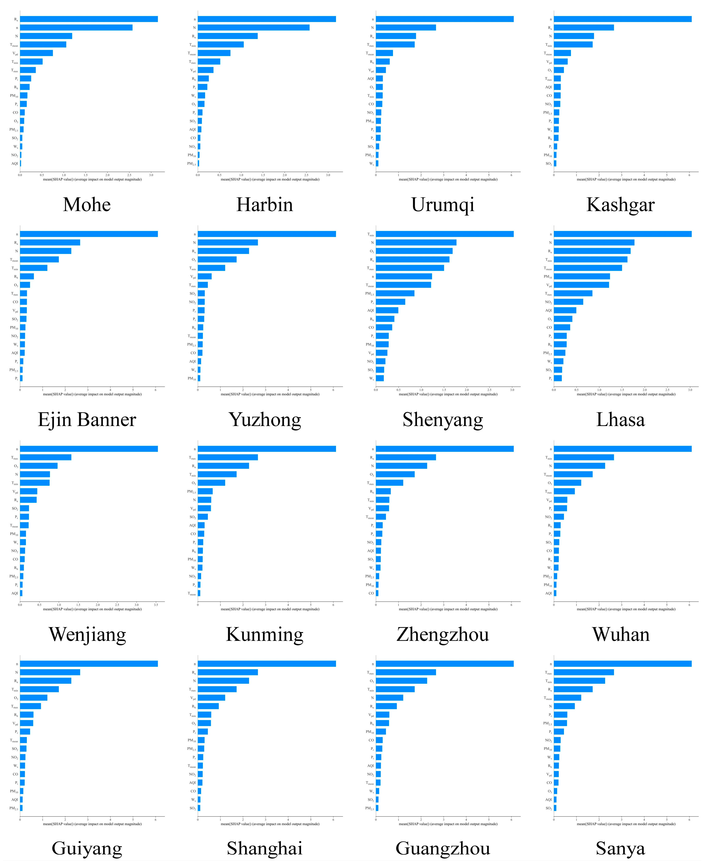
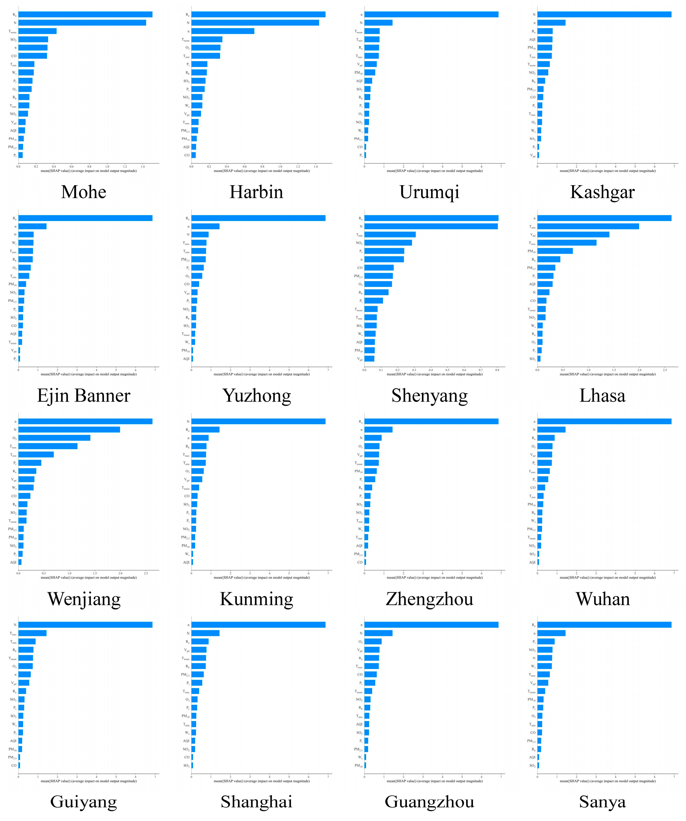
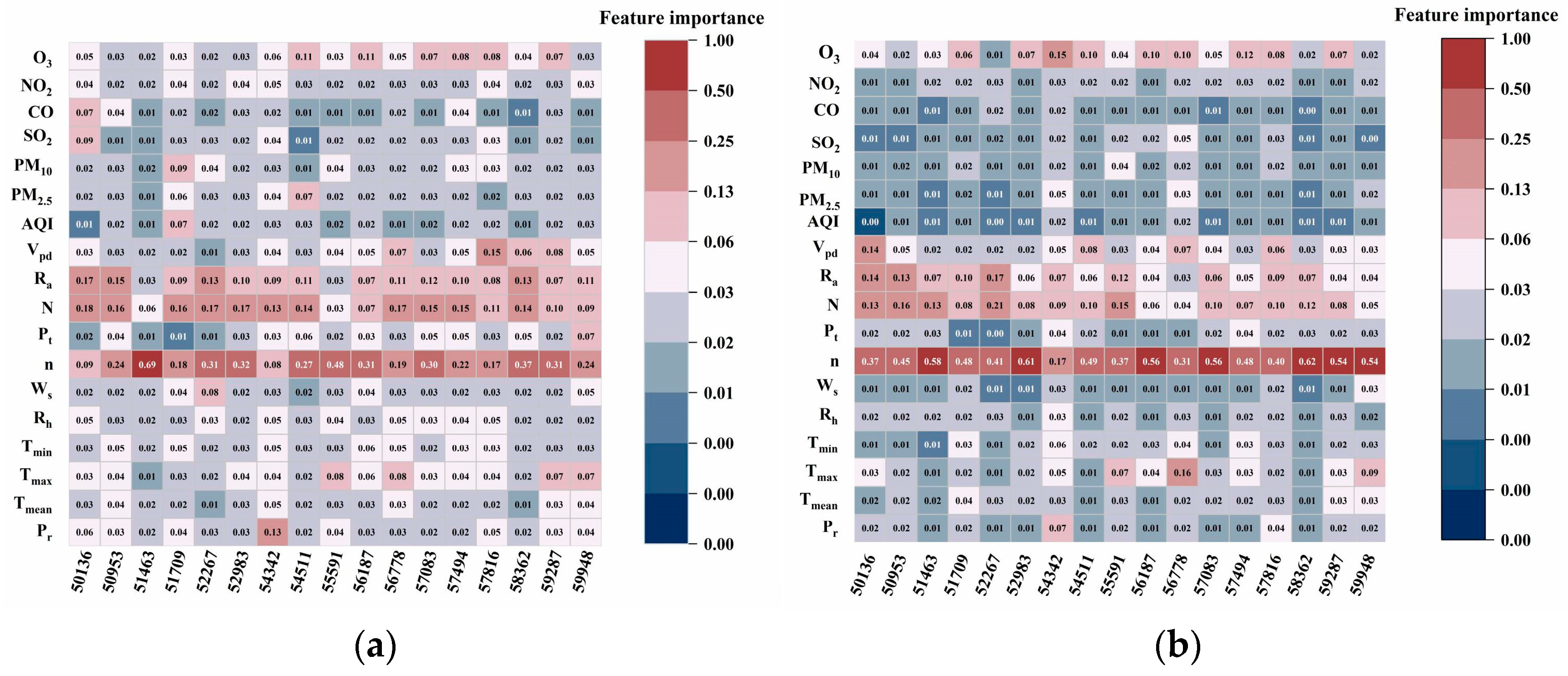
3.1. Selection Results of the CatBoost Feature Selection Algorithm

The results of feature selection using CatBoost to predict Rs and Rd are shown in Figure 4. The figure shows that n is the most critical factor affecting Rs, and the mean value and range of its importance are 0.47 (0.17–0.62). The results of the Rd feature selection show that n is the most important factor influencing Rd, and it is the first influencing factor in all regions except Mohe and Shenyang. The mean and range of its importance are 0.28 (0.08–0.69), and n is the second most important influencing factor in Mohe and Shenyang. N is the primary influencing factor of Rd in Mohe and Shenyang, and the feature importance values are 0.18 and 0.13, respectively. N and Ra performed better in calculating the characteristic importance of Rs and Rd than other factors except for n. The mean and range of the importance of Rs were 0.10 (0.04–0.21) and 0.08 (0.03–0.17), respectively, and the mean and range of the importance of Rd were 0.13 (0.03-–0.17) and 0.10 (0.03–0.15), respectively. This result is attributable to n being the most direct factor affecting radiation, whereas N and Ra are closely related to n. Although temperature-related characteristics can indirectly reflect cloud cover, the relationship between radiation and temperature is weaker than that between radiation and n [61,62]. Utilizing O3 data yields better performance than when other air pollution and meteorological data are utilized (except n, N, Ra), as revealed in the Rs and Rd of the characteristic importance calculation results. The mean value of its importance between 0.06 (0.01–0.15) and 0.05 (0.02–0.11) yields this result because Rd is the solar radiation passing through airborne substances, such as aerosols and molecules in the air scattered and formed by diffuse reflection from the surface, and O3 can scatter and absorb solar radiation, thus reducing the solar radiation reaching the Earth’s surface. Therefore, introducing air pollution is important for solar radiation prediction, which is consistent with the findings of previous studies, such as that by Mohammadi et al. [63], who evaluated the influence of nine characteristic factors on the prediction of daily radiation in Iran using the ANFIS model. They showed that n, N, and Ra are the most influential input parameters for predicting Rs and Rd. Furthermore, Fan et al. [64] confirmed that air pollution improves Rd prediction accuracy. The specifics of the feature ranking slightly differ among stations, presumably due to the geographical location and climatic differences among stations.
The greater the importance of the input variable, the higher the correlation between the variable and the output prediction, and removing less important features can reduce redundancy [65]. Finally, the median of the number of factors was selected as the threshold value, and feature screening was conducted for Rs and Rd to construct the Rs and Rd prediction models. The screening results are listed in Table A1.

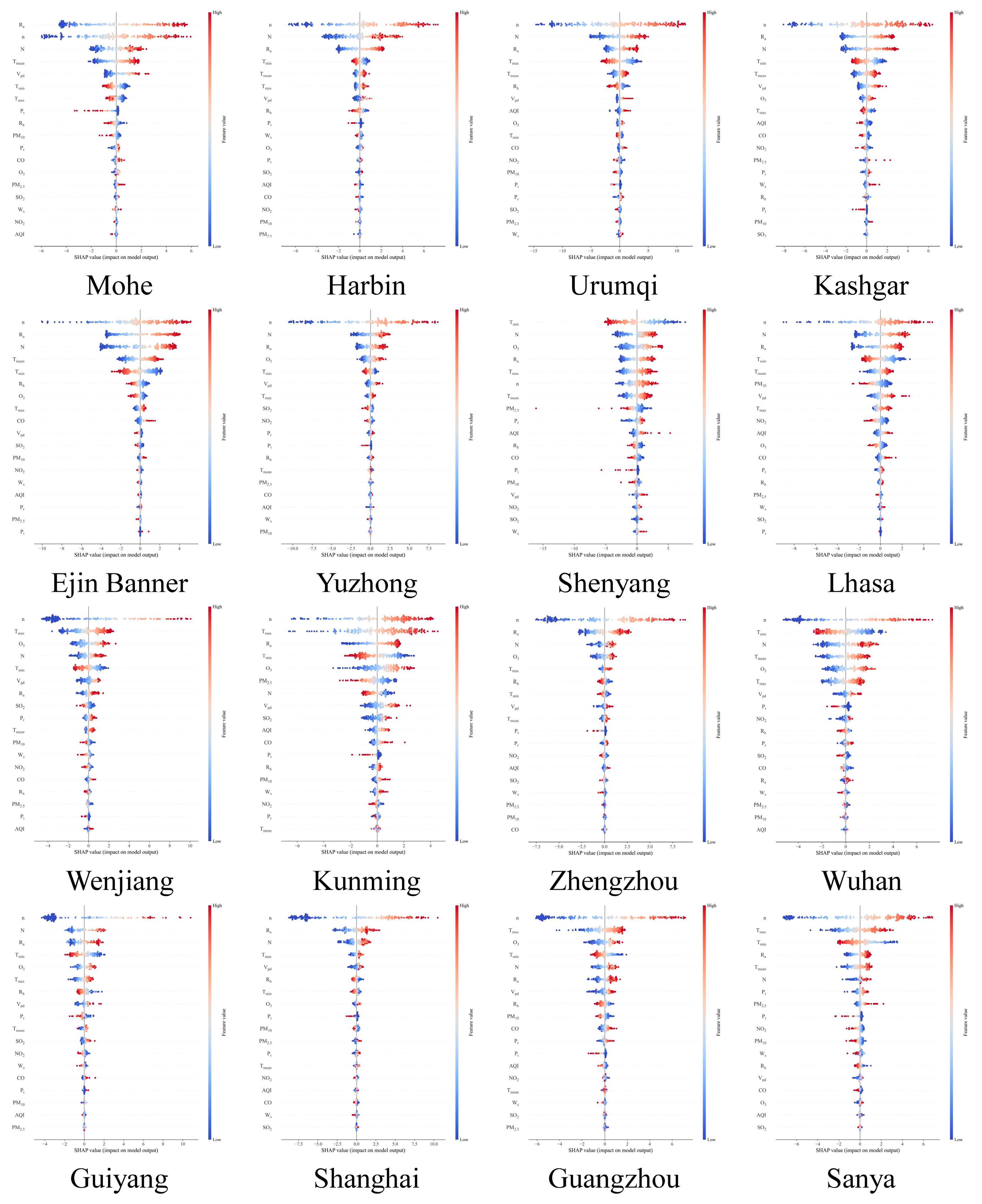
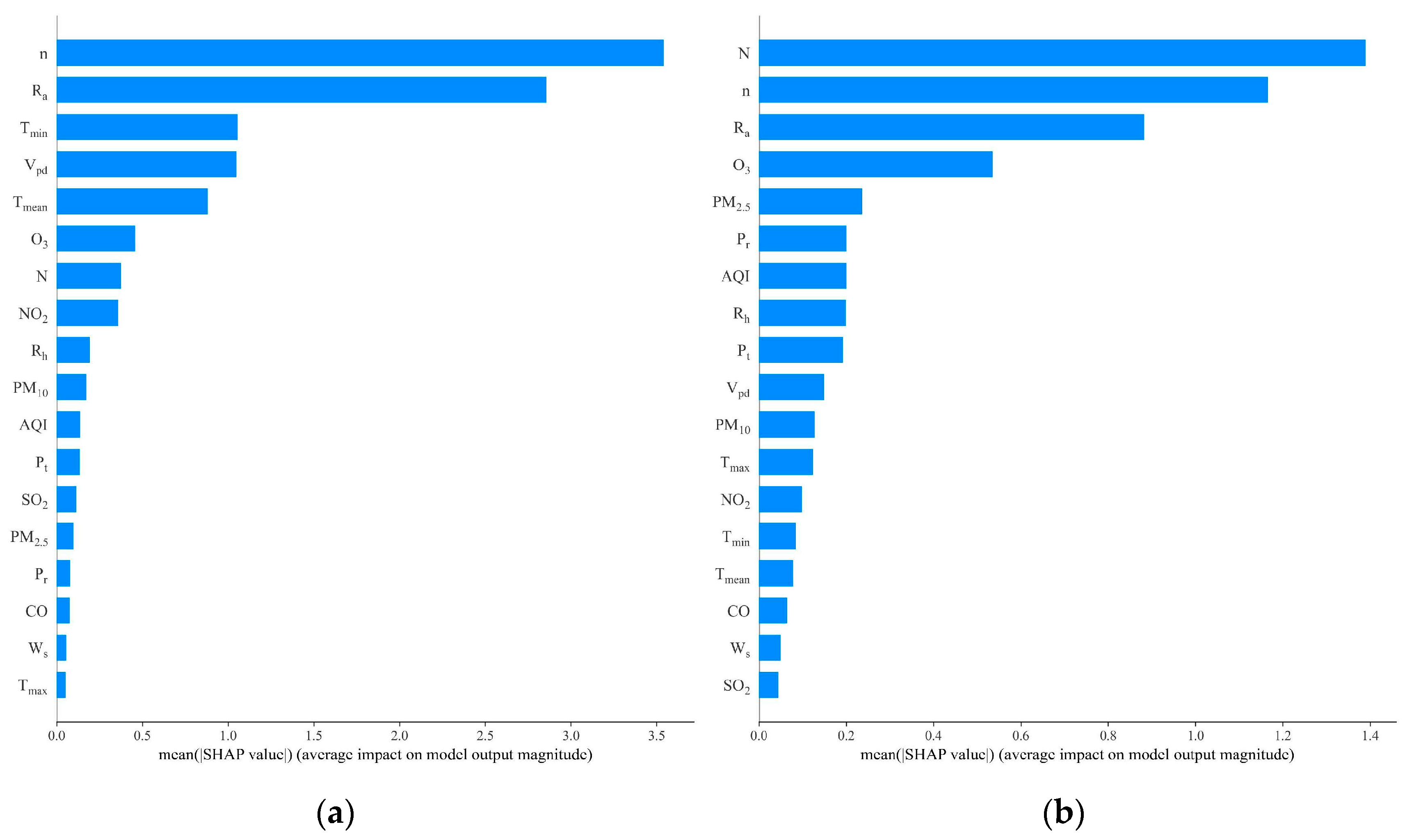
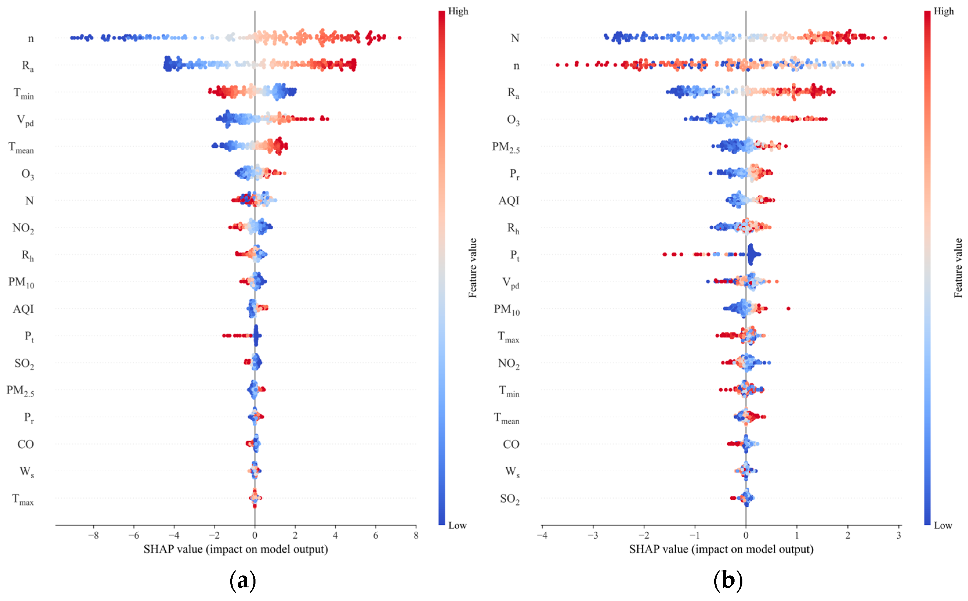
3.2. Shapley Additive Explanation (SHAP) Analysis

Traditional feature importance interpretation methods only explain the importance of features without elucidating how these features affect the prediction results. Therefore, this study introduced SHAP technology as a supplement to the explanatory analysis of the constructed stacking model. SHAP can not only reflect the degree of influence of each feature in each sample on the results but also how each feature affects the results and the positive and negative aspects of the influence [47]. Beijing is taken as the representative region, with other regions illustrated in Figure A1, Figure A2, Figure A3 and Figure A4. Figure 5 shows the mean absolute SHAP values of the stacking model. n indicates the highest mean SHAP value of 3.54 when the stacking model predicts Rs, followed by Ra with a mean SHAP value of 2.86, and Tmax has a lower mean SHAP value of 0.05. N exhibits the highest mean SHAP value of 1.39 for predicting Rd, followed by n with a mean SHAP value of 1.17, and SO2 has a lower mean SHAP value of 0.04.
The global interpretation in Figure 6 reveals that the first 14 features (n, Ra, Tmin, Vpd, Tmean, O3, N, NO2, Rh, PM10, AQI, Pt, SO2, and PM2.5) have a dominant influence on radiation regarding the stacking model prediction of Rs. The last four features (Pr, CO, Ws, and Tmax) are mostly concentrated in the nearby 0 SHAP, indicating that these features have little influence on radiation prediction for most days. When predicting Rd using the stacking model, the first 13 features (N, n, Ra, O3, PM2.5, Pr, AQI, Rh, Pt, Vpd, PM10, Tmax, and NO2) have a significant influence on radiation. The last five features (Tmin, Tmean, CO, Ws, and SO2) are concentrated around 0 SHAP. The most important features in the SHAP value ranking are those related to sunshine duration (n, N, and Ra), and the larger their values, the larger the corresponding SHAP values. This shows that the larger these eigenvalues are, the larger the solar radiation is. The absolute value of SHAP of the temperature feature when predicting Rs is higher than that of predicting Rd, indicating that the contribution of the temperature feature set to the prediction of Rs is greater than that of Rd. The rainfall features for some days also have a considerable effect on radiation prediction, and the smaller the value, the smaller the solar radiation prediction value, which is consistent with the intuition of rainfall being closely related to cloud cover and clouds diminishing solar radiation. And several studies have shown the same conclusion that rainfall has a definite effect on radiation estimates [62,66,67]. Regarding air pollution characteristics, a larger O3 value has a greater influence on radiation prediction. Introducing O3 can improve the prediction accuracy of solar radiation because the ozone layer absorbs a large amount of radiation [45].

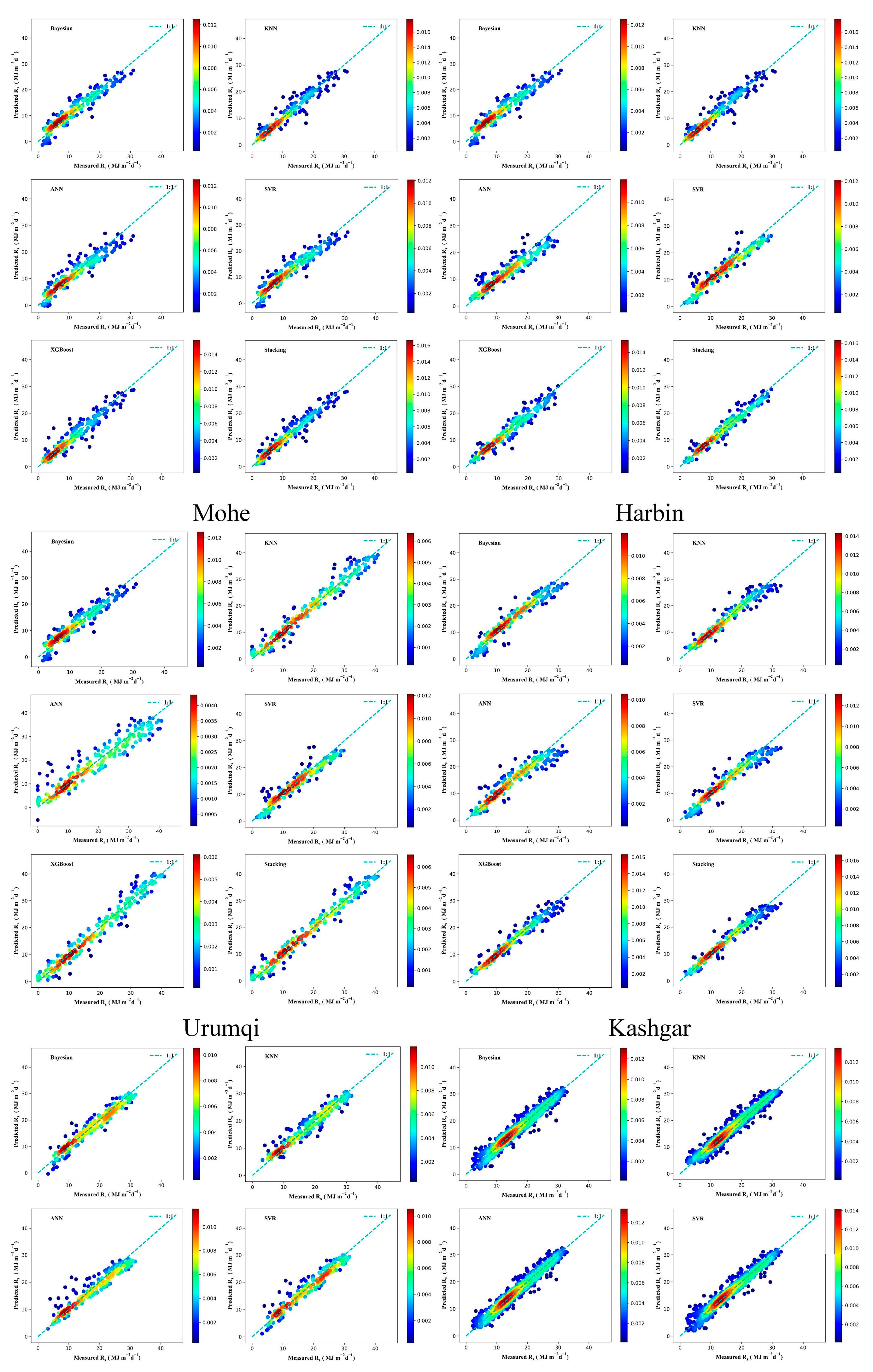
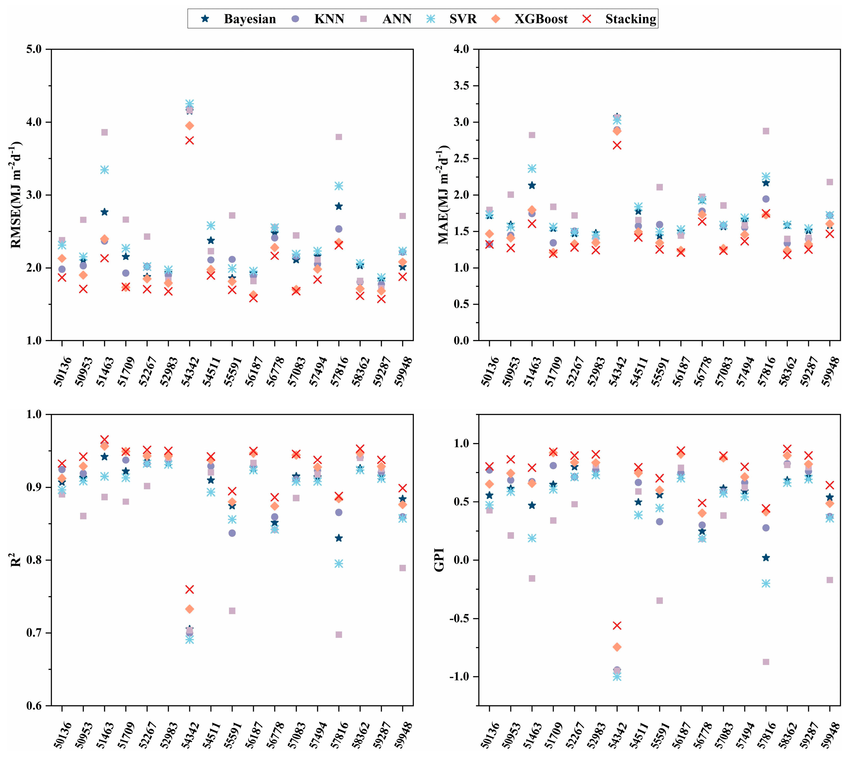
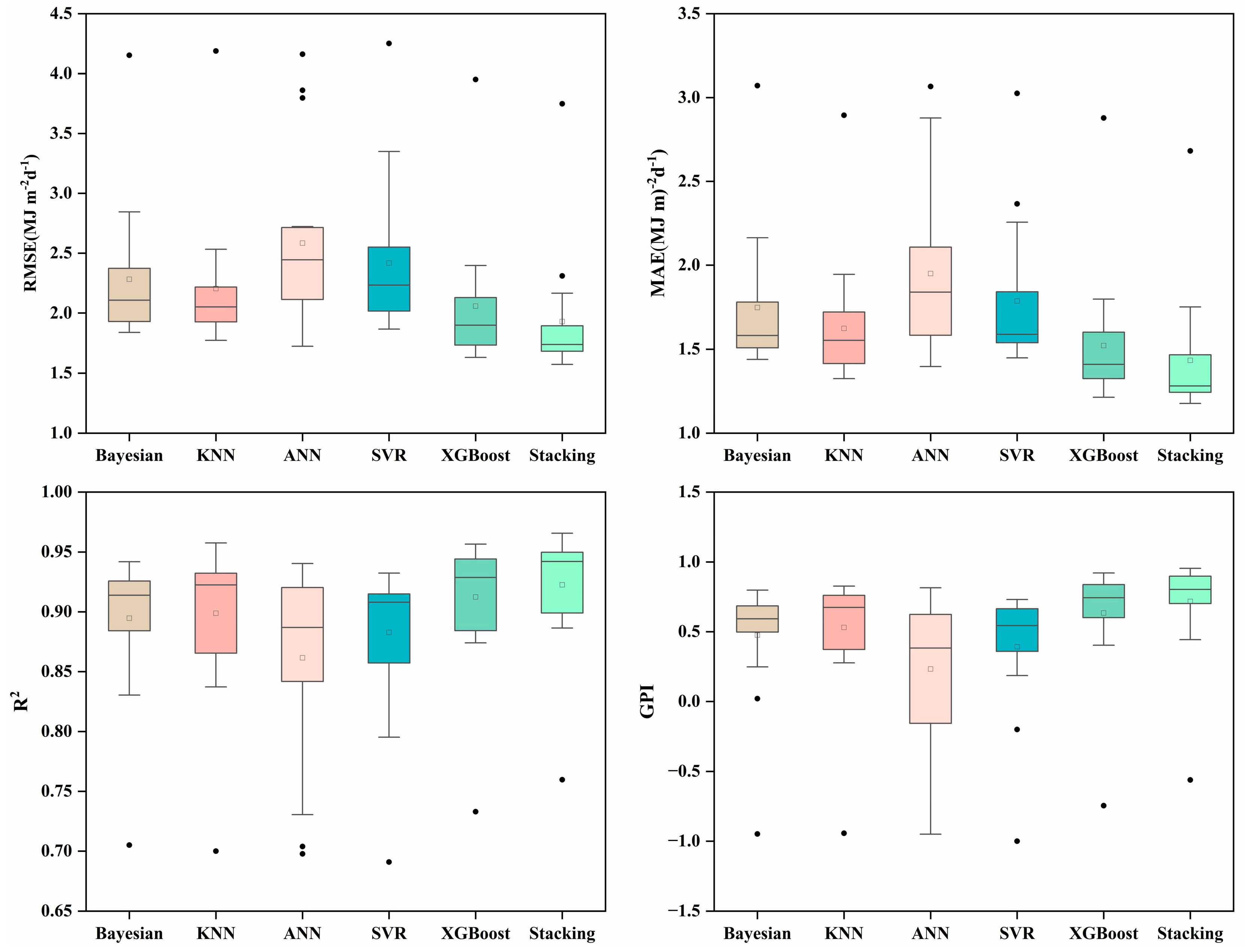
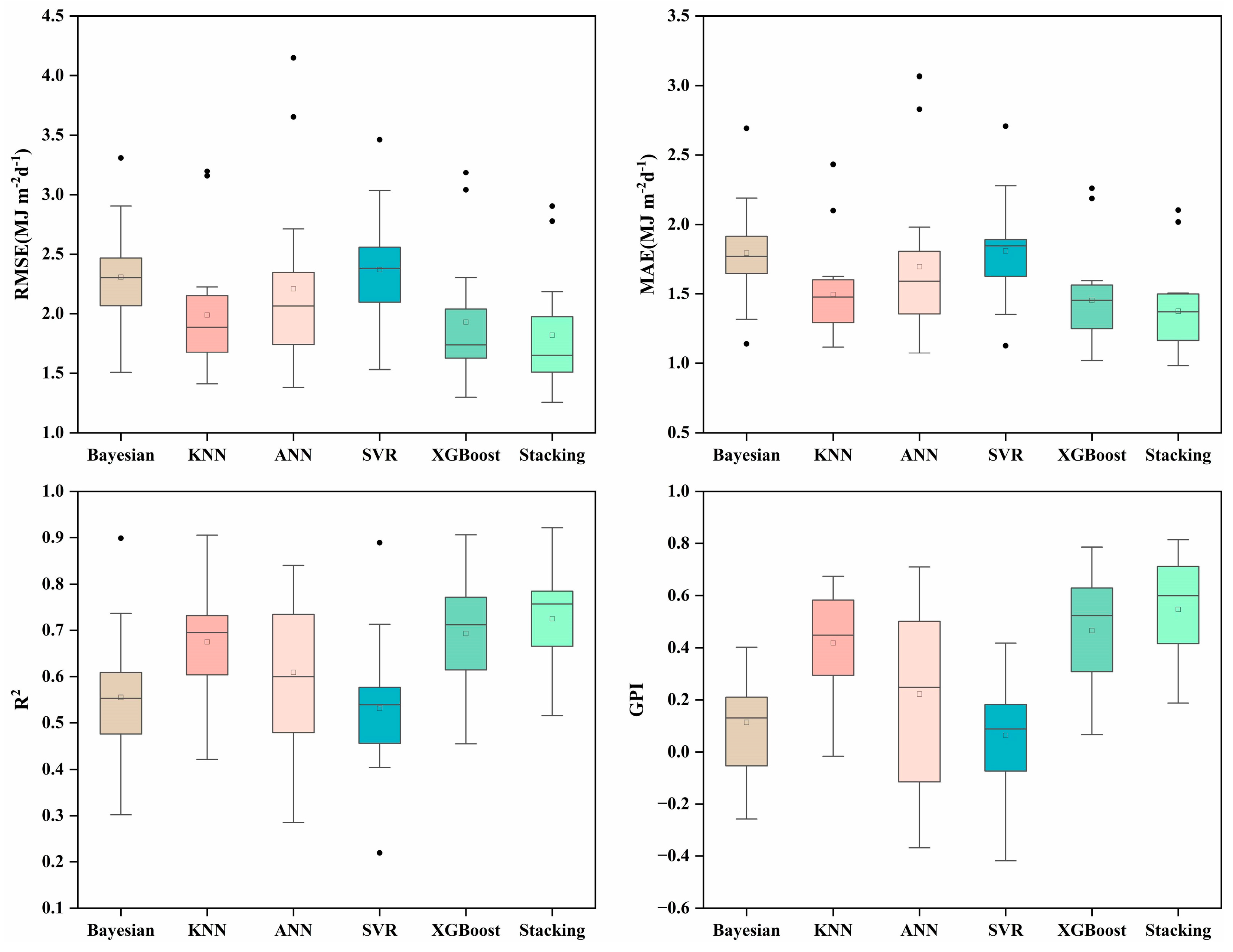
3.3. Performance of Different ML Models in Radiation Estimation

Seventeen radiation stations in different regions of China were considered. After applying the CatBoost feature selection algorithm, the selected features were further input into different models. The results of these models in the testing phase are shown in Table A2. Figure 7 and Figure 8, and Table A2 reveal that XGBoost and KNN performed better than the other base learners, and the range and mean values of the XGBoost model RMSE, MAE, R2, and GPI in predicting Rs were 1.6322–3.9516 (2.0580), 1.2141–2.8782 (1.5218), 0.7330–0.9564 (0.9124), and from −0.7450 to 0.9210 (0.6326), respectively. The ranges and means of the RMSE, MAE, R2, and GPI of the KNN models were 1.7749–4.1885 (2.2043), 1.3251–2.8946 (1.6244), 0.7000–0.9575 (0.8988), and from −0.9434 to 0.8271 (0.5165), respectively. The ranges and means of the RMSE, MAE, R2, and GPI of XGBoost models for predicting Rd were 1.2996–3.1848 (1.9300), 1.0189–2.2588 (1.4250), 0.4551–0.9058, (0.6932) and 0.0665–0.7855 (0.4659), respectively. The ranges and means of the RMSE, MAE, R2, and GPI of the KNN models were 1.4109–3.1970 (1.9891), 1.1182–2.4330 (1.4688), 0.4216–0.9051 (0.6753), and from −0.0161 to 0.6746 (0.4186), respectively. Because XGBoost is an ensemble learning method, it can accurately upgrade a weak learner to a stronger learner by integrating multiple base models to solve the problem. Its high training speed and strong generalization ability make it a popular choice [68]. XGBoost expands the loss function by Taylor’s second order and utilizes the first- and second-order derivatives for updating and iterating during optimization; the model makes full use of the data. Therefore, selecting a base learner with good performance improves the overall performance of the ensemble model [61,69]. The stacking model had the highest accuracy for predicting Rs. The range and mean values of RMSE, MAE, R2, and GPI were 1.5737–3.7482 (1.9318), 1.1773–2.6814 (1.4336), 0.7597–0.9655 (0.9226), and from −0.5614 to 0.9542 (0.7122), respectively. Stacking had an RMSE and MAE mean reduction range of 6.14%–25.25% and 5.79%–26.48%, respectively, and the R2 mean improvement range was 1.12%–7.09%. The range and mean values of RMSE, MAE, R2, and GPI for the highest accuracy in predicting Rd compared to the base learner were 1.2589–2.9038 (1.8201), 0.9811–2.1024 (1.3493), 0.5153–0.9217 (0.7248), and from 0.1877 to 0.8135 (0.5472), respectively. Stacking had an RMSE and MAE mean reduction range of 5.70%–23.27% and 5.31%–24.30%, respectively, and the R2 mean improvement range was 4.56%–36.24%, demonstrating that the accuracy improvement in stacking is great, and the ensemble learning model construction is effective.
Figure 9 and Figure 10 demonstrate that the stacking model is closer to the 1:1 line in the data points in the scatter plot, indicating its higher accuracy. See Figure A5 and Figure A6 for scatter plots in other regions. The stacking model results for Rs and Rd prediction are represented by box plots in Figure 11 and Figure 12, respectively, and the 50th percentile (P50) was used as the benchmark for evaluation. The higher P50 is, the better the mean performance of the whole model. The P50 values of RMSE in predicting Rs for the Bayesian, KNN, ANN, SVR, XGBoost, and stacking models at 17 stations were 2.1074, 2.0503, 2.4454, 2.2331, 1.9013, and 1.7402 MJ m−2d−1, respectively; the P50 values of MAE were 1.5825, 1.5531, 1.8388, 1.5891, 1.4095, and 1.2810 MJ m−2d−1; the P50 values of R2 were 0.9138, 0.9225, 0.8869, 0.9080, 0.9287, and 0.9421; and P50 values of GPI were 0.5922, 0.6669, 0.3406, 0.5443, 0.7435, and 0.7989, respectively. Additionally, The P50 values of RMSE in predicting Rd for the Bayesian, KNN, ANN, SVR, XGBoost, and stacking models were 2.3032, 1.8867, 2.0640, 2.3815, 1.7395, and 1.6492 MJ m−2d−1; the P50 values of MAE were 1.7705, 1.3968, 1.5253, 1.8120, 1.3221, and 1.2413 MJ m−2d−1; the P50 values of R2 were 0.5533, 0.6951, 0.5996, 0.5394, 0.7118, and 0.7567; and P50 values of GPI were 0.1297, 0.4480, 0.2476, 0.0884, 0.5231, and 0.5988, respectively. The base learners are ranked according to performance as XGBoost > KNN > ANN > Bayesian > SVR. The Taylor diagram in Figure 13 and Figure 14 visualizes the performance of different models estimating Rs and Rd in Beijing. Taylor diagrams for other regions are in Figure A7 and Figure A8. Obviously, the stacking model is closer to the observation point and has better performance than other models. These results confirm that the proposed stacking ensemble model achieves satisfactory accuracy in predicting Rs and Rd. By choosing models with diverse principles and less correlation, data with different data frames and spatial dimensions can be observed and the corresponding models can be constructed according to the principles of the algorithm itself [43]. Selecting algorithms with divergent principles complements the differentiation of the models, thus utilizing their strengths and overcoming their weaknesses [29].

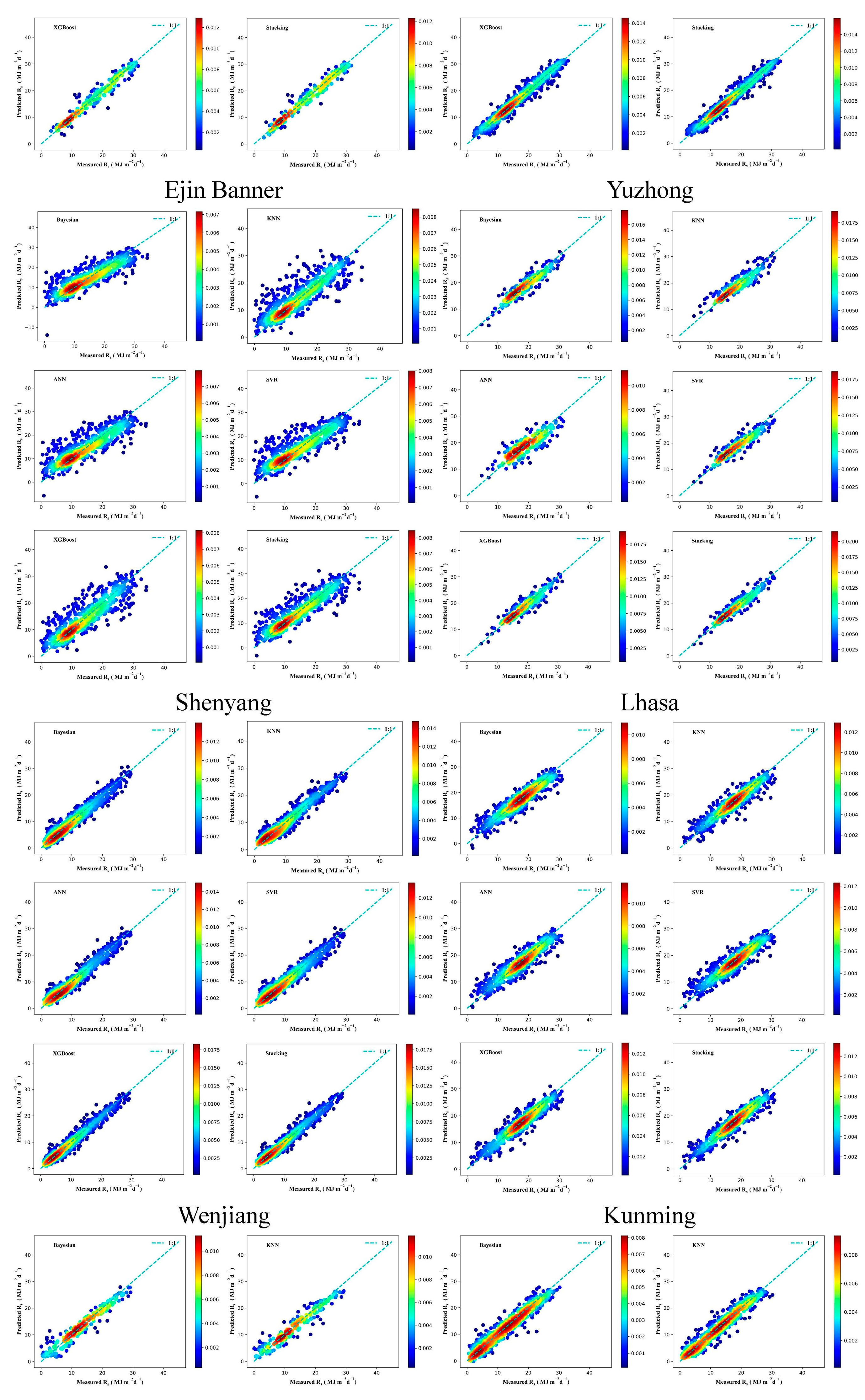
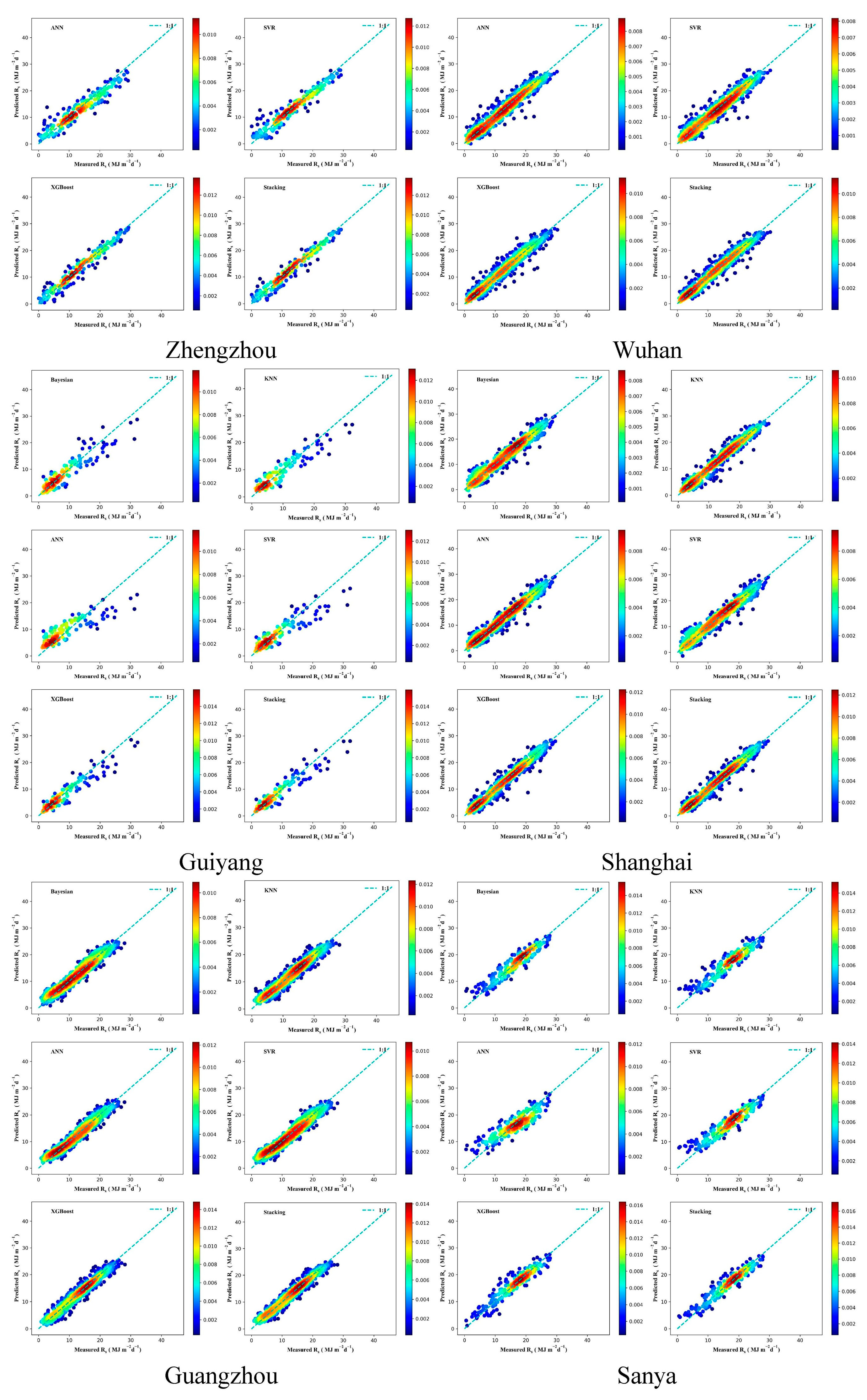
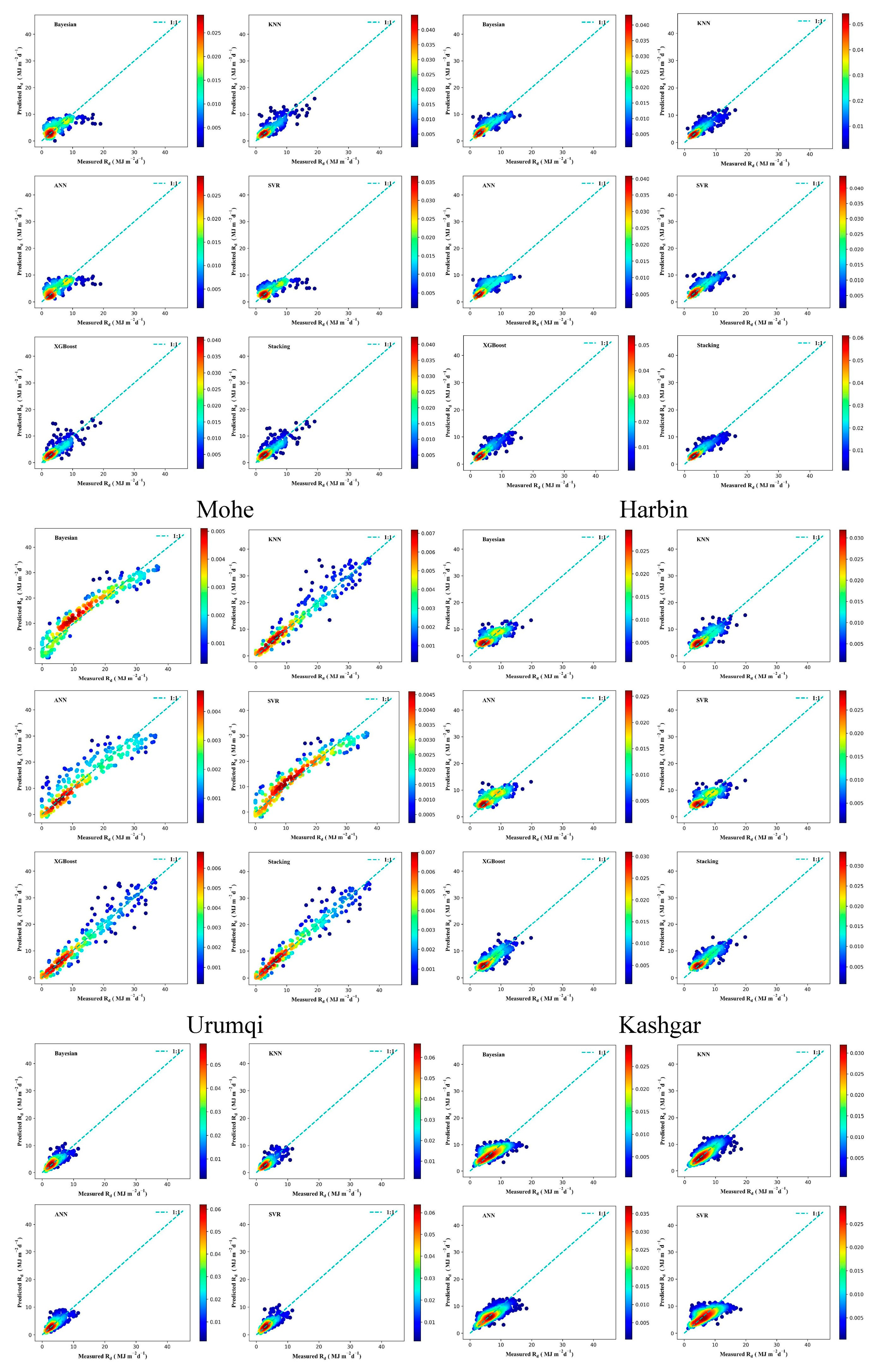
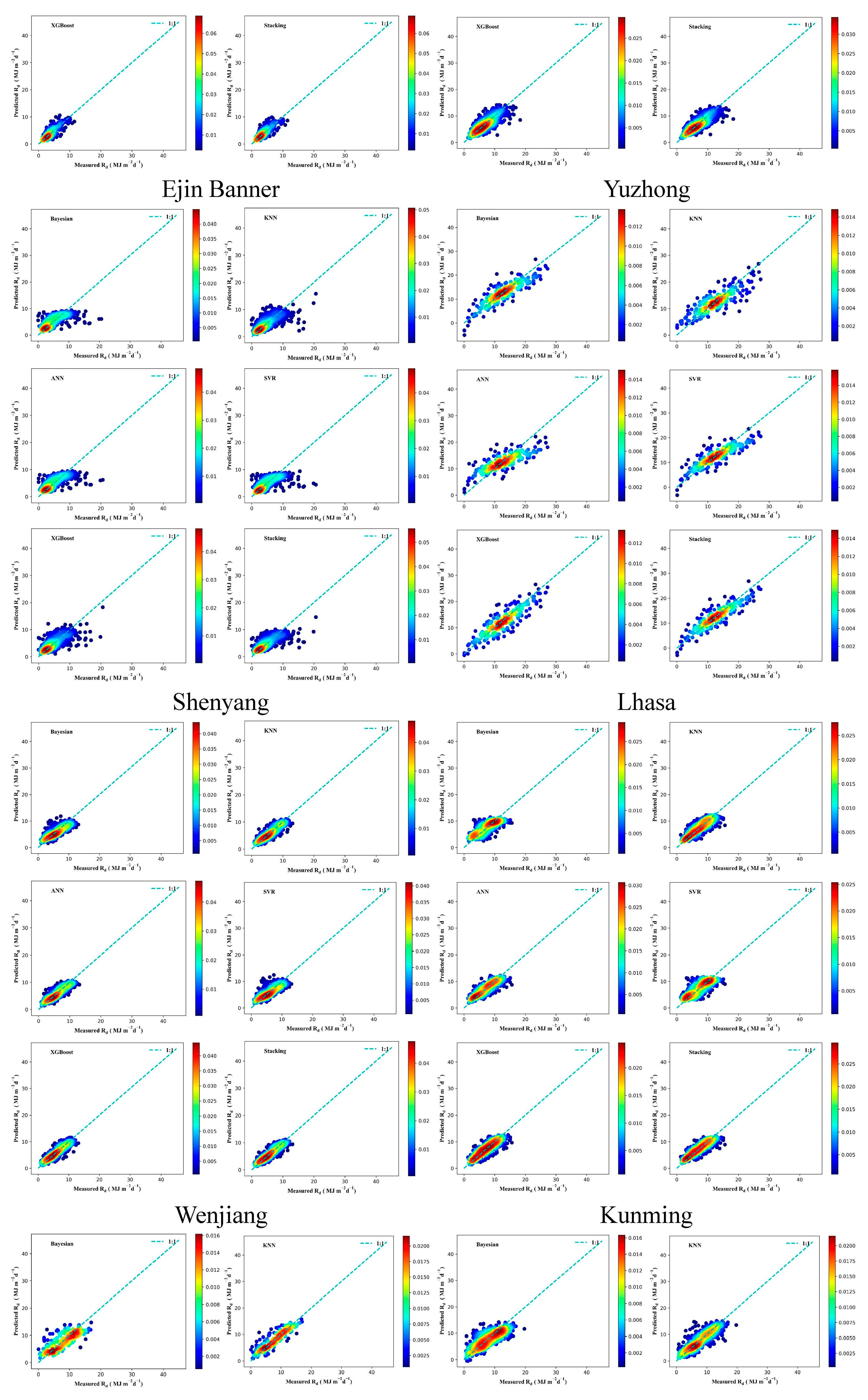
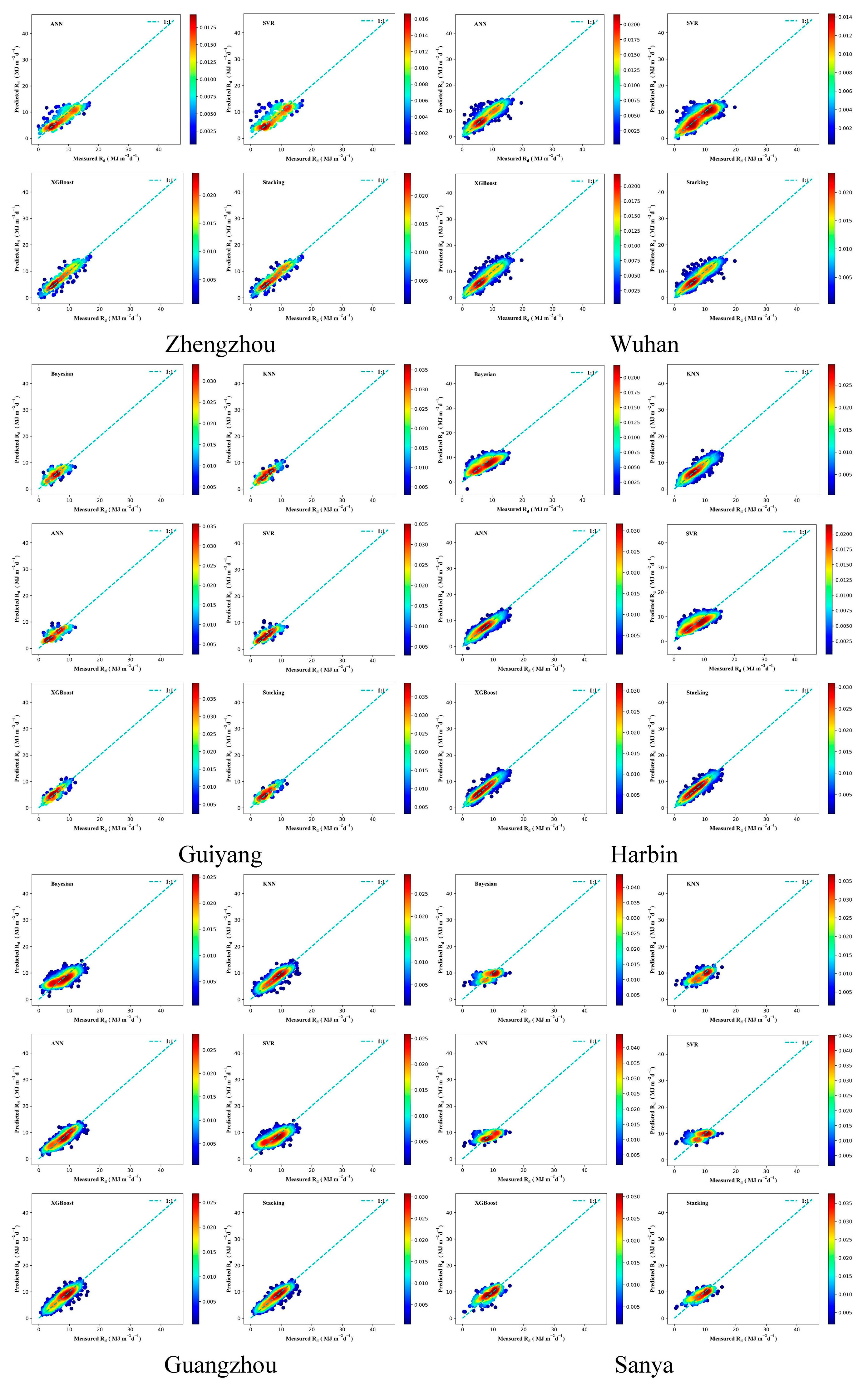
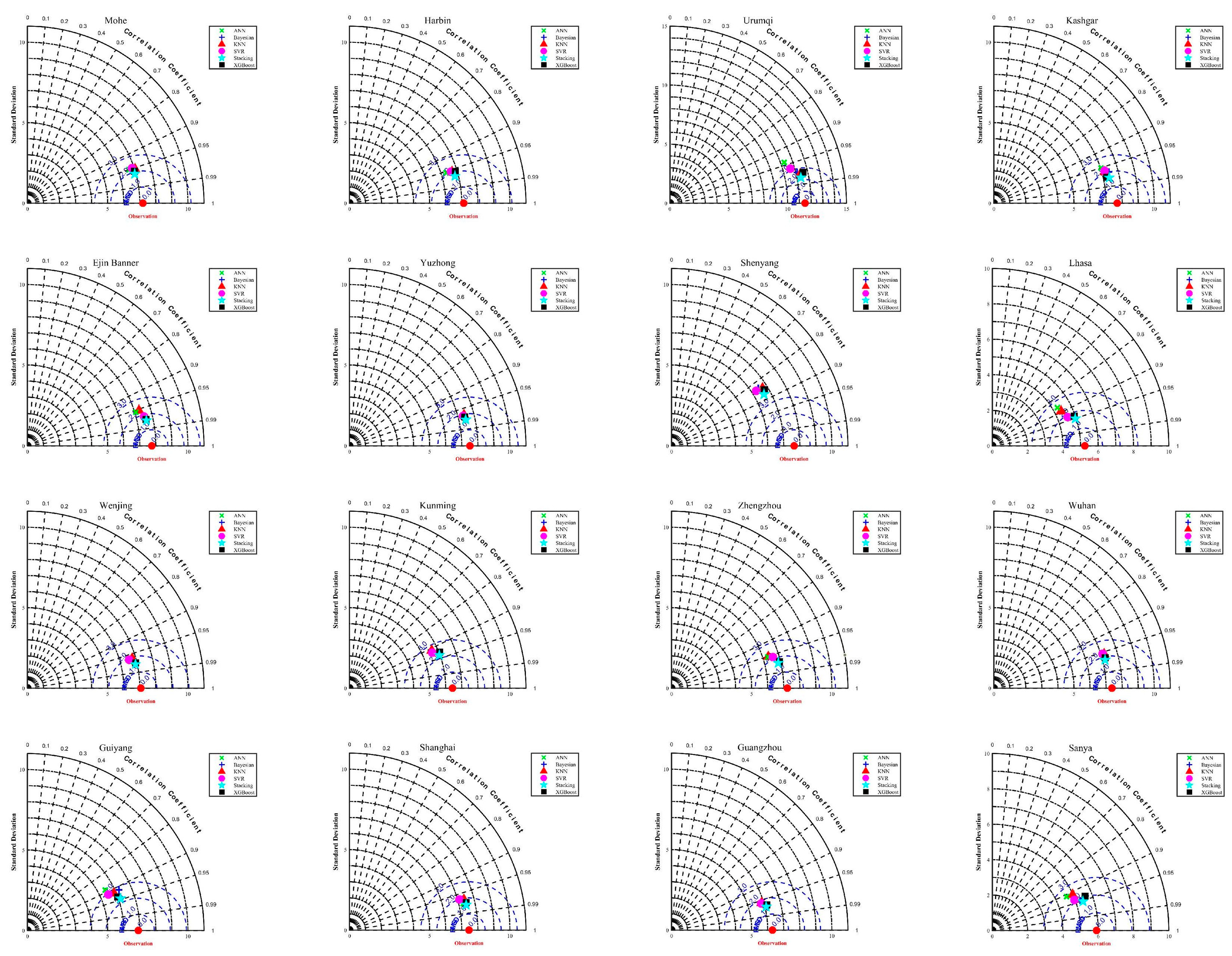
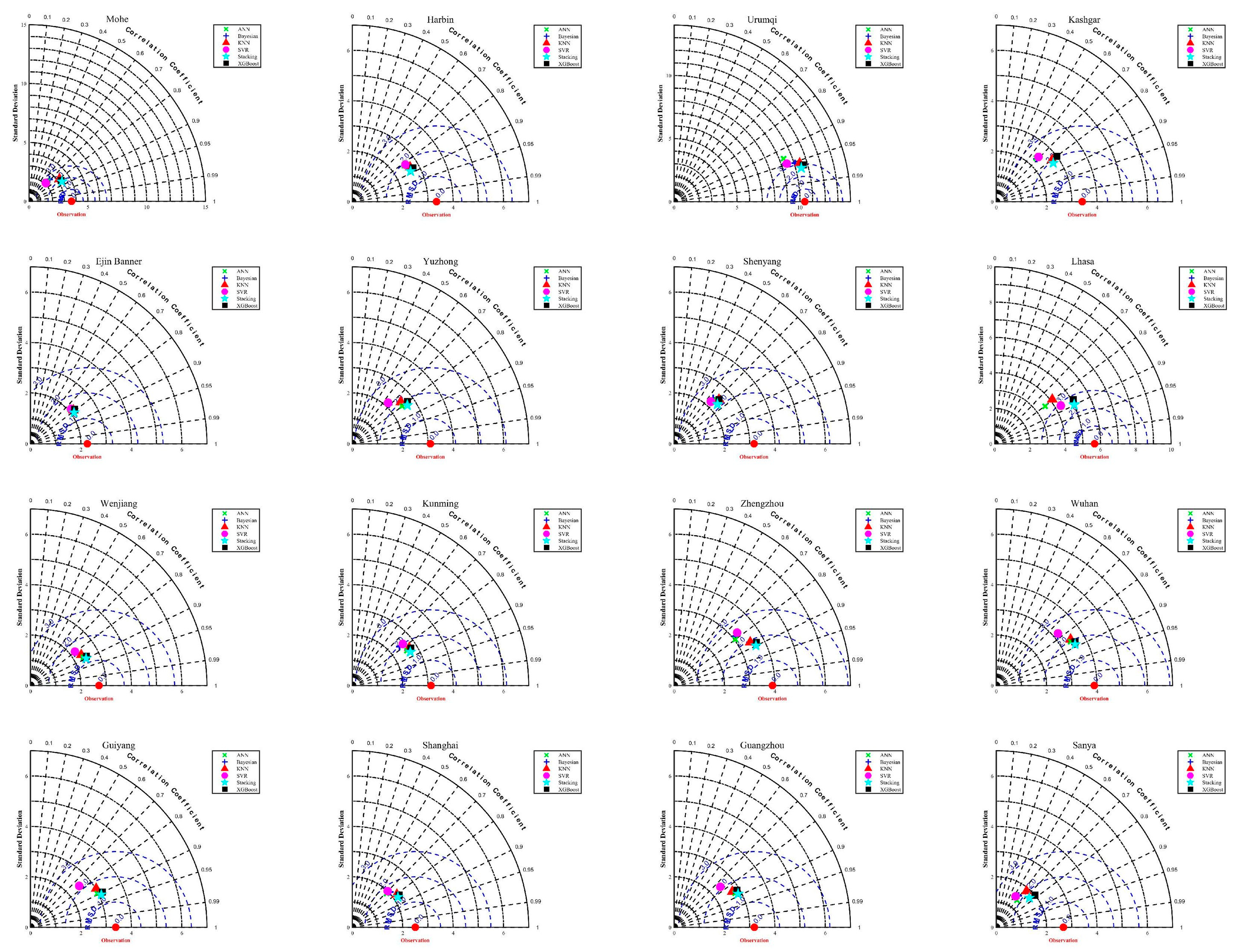
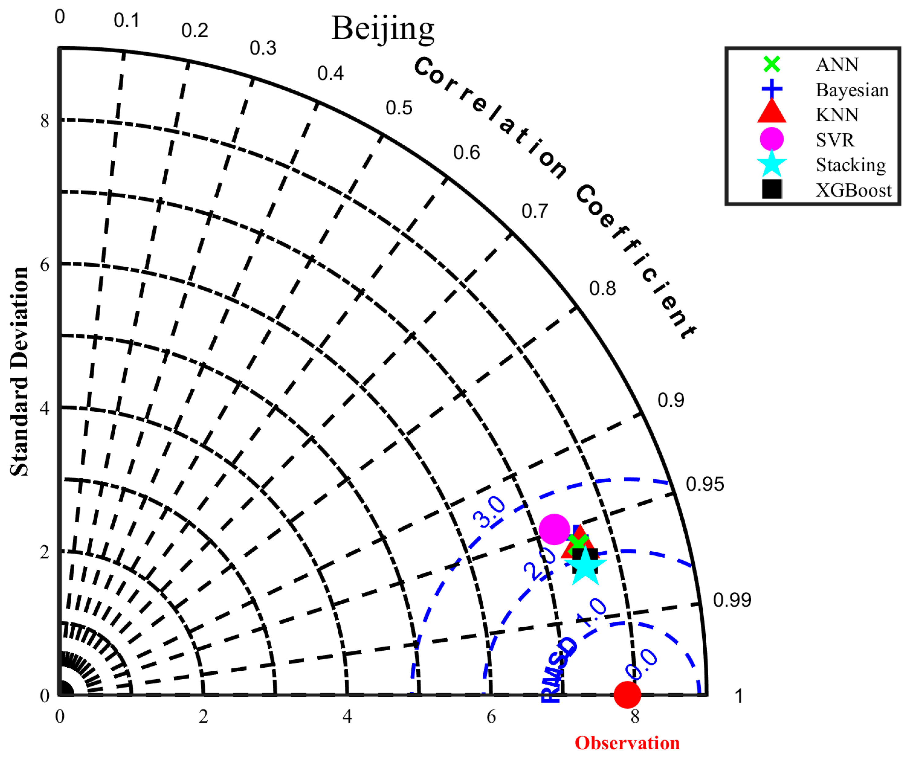
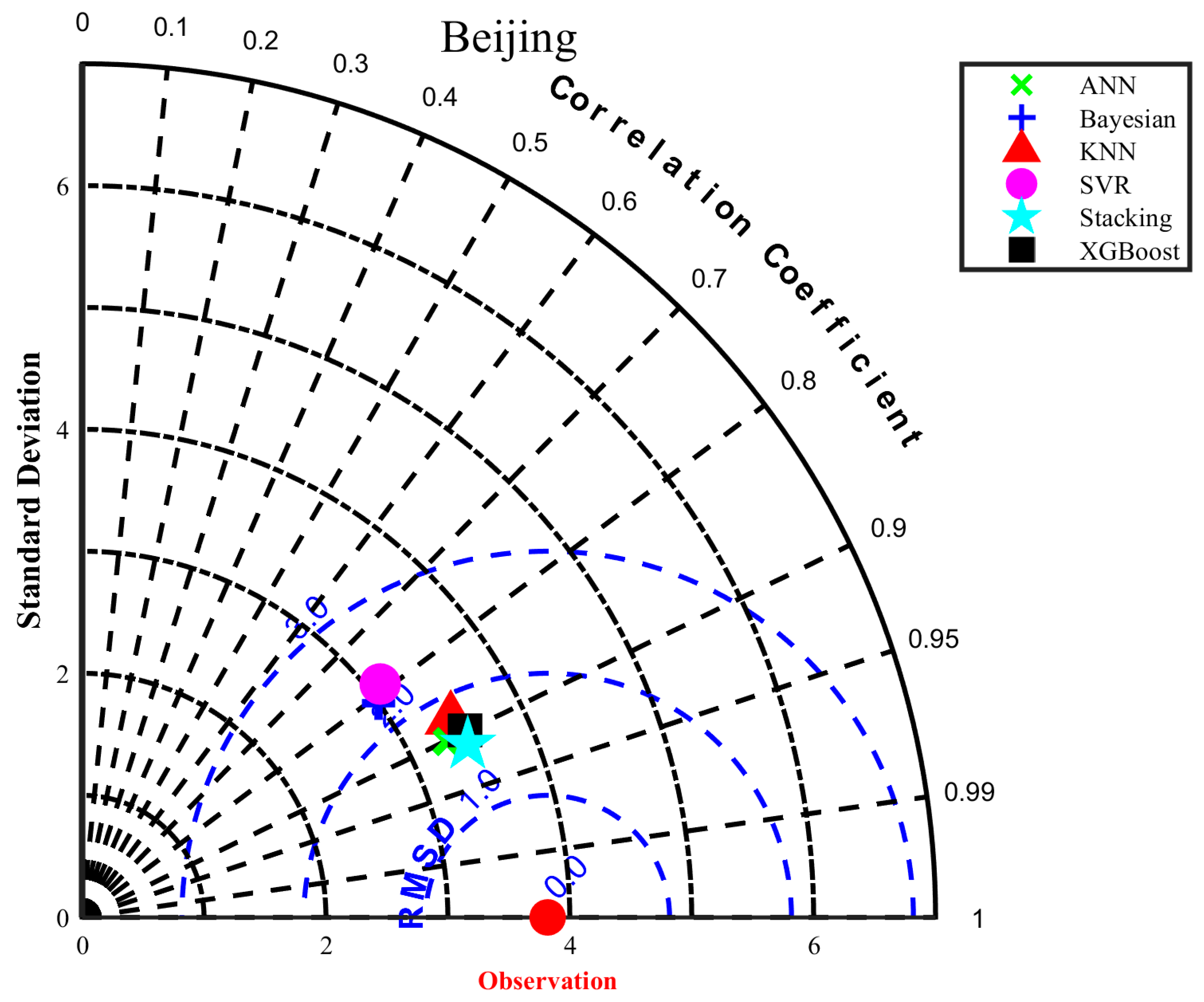
3.4. Solar Radiation Performance of the Stacking Model in Different Regions

Figure 8 and Table A2 reveal that in predicting Rs using the stacking model, the precision is highest in coastal areas, such as Shanghai and Guangzhou, except in Sanya. The ranges of RMSE, MAE, R2, and GPI are 1.5737–1.6160, 1.1773–1.2529, 0.9375–0.9530, and 0.8980–0.9542, respectively. The values of RMSE, MAE, R2, and GPI in Sanya are 1.8783, 1.4672, 0.8989, and 0.6438, respectively. In inland areas, the results were better in Wenjiang, where RMSE, MAE, R2, and GPI were 1.5830, 1.2111, 0.9498, and 0.9394, respectively. The worst accuracy was observed in Shenyang, where the RMSE, MAE, R2, and GPI were 3.7482, 2.6814, 0.7597, and −0.5614, respectively. Figure 12 and Table A2 reveal that in predicting Rd using the stacking model, the precision is highest in coastal areas, such as Shanghai and Guangzhou, except in Sanya. The range of GPI is 0.7123–0.8135. In the inland area, the Wenjiang area performed better, with a GPI of 0.8055. Shenyang has the worst accuracy with a GPI of 0.1877. This is consistent with the findings of Jia et al. [70], who evaluated the performance of three common ML algorithms (linear modeling, SVR, and RF), in solar radiation estimation in eight cities in China. The results demonstrated that the performance of the model in coastal areas was higher than that in inland areas. Wang et al. [71] obtained similar results when using 97 empirical models to predict the Rd of 17 cities in China; that is, the accuracy of the model was higher in coastal areas, but the performance of the rainy-weather model in Sanya was poor. Presumably, air conditions may deteriorate the model accuracy in some inland areas.

4. Conclusions

In this study, 17 typical radiation stations in China are selected, and meteorological data and air pollution data are collected. The characteristic Rs and Rd factors are determined using the CatBoost feature selection algorithm, and the daily Rs and Rd prediction models are constructed by combining the proposed stacking. The SHAP value is used to explain the ensemble model and verify the reliability of the feature selection algorithm. The main conclusions of this study are as follows:
(1)
Among the meteorological factors, n and its related characteristics (Ra and N) have the greatest influence on the prediction of solar radiation (Rs, Rd), whereas O3 has the greatest influence on the air pollution data. The most important feature is n, and the higher its value, the greater the influence on the radiation prediction. Regarding air pollution characteristics, a larger O3 value implies a greater effect on radiation prediction.
(2)
Compared with base learners, the proposed stacking model performs optimally with a mean improvement range of 5.70%–25.25% for RMSE, 5.31%–26.48% for MAE, and 1.12%–36.24% for R2, thus highlighting the necessity of ensemble learning model construction.
(3)
This study provides a reference for selecting predicted radiation input characteristics in different climatic regions in China. Notably, the accuracy of the proposed stacking model in coastal areas (Shanghai and Guangzhou) is better than that in inland regions.

Author Contributions

Y.D.: conceptualization, methodology, validation, writing—original draft. Y.W.: conceptualization, writing—original draft, investigation, validation, formal analysis. Z.L.: data curation, writing—review and editing, validation, formal analysis. L.Z.: data curation, software, funding acquisition. Y.S.: data curation, Supervision. S.C.: data curation. X.X.: supervision, project administration. All authors have read and agreed to the published version of the manuscript.

Funding

This work was supported by the National Natural Science Foundation of China (No. 52309050 and 32372680), the Ph.D. Research Startup Foundation of Henan University of Science and Technology (No. 13480025 and 13480033), Key R&D and Promotion Projects in Henan Province (Science and Technology Development) (No. 232102110264), Henan Provincial Tobacco Company Luoyang City Company Technology Innovation Pro (No. 2023410300200043), Key Scientific Research Projects of Colleges and Universities in Henan Province (No. 24B416001), and the Innovative Research Team (Science and Technology) in the University of Henan Province (23IRTSTHN024).

Institutional Review Board Statement

Not applicable.

Informed Consent Statement

Not applicable.

Data Availability Statement

The original contributions presented in this study are included in the article. Further inquiries can be directed to the corresponding authors.

Acknowledgments

For this study, we are grateful to the National Meteorological Information Centre of the China Meteorological Administration for supplying the climate database.

Conflicts of Interest

The authors declare no conflicts of interest.

Nomenclature

AQIair quality index
COcarbon monoxide
GPIglobal performance index
MAEmean absolute error
nsunshine duration
Nmaximum sunshine duration
NO2nitrogen dioxide
O3ozone
Prair pressure
Ptprecipitation
R2coefficient of determination
Raextra-terrestrial solar radiation
Rddiffuse solar radiation
Rhrelative humidity
RMSEroot mean square error
Rsglobal solar radiation
SO2sulfur dioxide
Tmaxmaximum temperature
Tmeanmean temperature
Tminminimum temperature
Vpdvapor pressure deficit
Wswind speed

Appendix A

(See Table A1 and Table A2).
Table A1. Results of CatBoost feature selection.
StationSelected Features
RsRd
Mohe‘n’, ‘Ra’, ‘Vpd’, ‘N’, ‘O3’, ‘Tmax’, ‘Pt’, ‘Rh’, ‘Pr‘N’, ‘Ra’, ‘SO2’, ‘n’, ‘CO’, ‘Pr’, ‘O3’, ‘Rh’, ‘NO2
Harbin‘n’, ‘N’, ‘Ra’, ‘Vpd’, ‘Tmean’, ‘O3’, ‘Pt’, ‘Rh’, ‘Tmax‘n’, ‘N’, ‘Ra’, ‘Tmin’, ‘Pt’, ‘Tmean’, ‘Tmax’, ‘CO’, ‘Pr
Urumqi‘n’, ‘N’, ‘Ra’, ‘O3’, ‘Pt’, ‘Rh’, ‘NO2’, ‘Vpd’, ‘Tmean‘n’, ‘N’, ‘Ra’, ‘O3’, ‘NO2’, ‘Rh’, ‘Ws’, ‘Pr’, ‘Tmin
Kashgar‘n’, ‘Ra’, ‘N’, ‘O3’, ‘Tmean’, ‘Tmin’, ‘Rh’, ‘Vpd’, ‘Ws‘n’, ‘N’, ‘Ra’, ‘PM10’, ‘AQI’, ‘PM2.5’, ‘Tmin’, ‘Ws’, ‘NO2
Ejin Banner‘n’, ‘N’, ‘Ra’, ‘NO2’, ‘Rh’, ‘Tmean’, ‘Vpd’, ‘CO’, ‘SO2‘n’, ‘N’, ‘Ra’, ‘Ws’, ‘PM10’, ‘Rh’, ‘PM2.5’, ‘Pr’, ‘SO2
Yuzhong‘n’, ‘N’, ‘O3’, ‘Ra’, ‘Tmax’, ‘Vpd’, ‘Tmin’, ‘Tmean’, ‘CO’‘n’, ‘N’, ‘Ra’, ‘Tmax’, ‘NO2’, ‘Tmin’, ‘Vpd’, ‘Pt’, ‘CO’
Shenyang‘n’, ‘O3’, ‘N’, ‘Ra’, ‘Pr’, ‘Tmin’, ‘PM2.5’, ‘Vpd’, ‘Tmax‘Pr’, ‘N’, ‘Ra’, ‘n’, ‘O3’, ‘NO2’, ‘Tmean’, ‘Tmin’, ‘Rh
Beijing‘n’, ‘N’, ‘O3’, ‘Vpd’, ‘Ra’, ‘Tmin’, ‘Pt’, ‘NO2’, ‘Rh‘n’, ‘N’, ‘Ra’, ‘O3’, ‘PM2.5’, ‘Pt’, ‘Rh’, ‘Vpd’, ‘NO2
Lhasa‘n’, ‘N’, ‘Ra’, ‘Tmax’, ‘PM10’, ‘O3’, ‘Tmean’, ‘Vpd’, ‘Rh‘n’, ‘Tmax’, ‘PM10’, ‘Rh’, ‘Pr’, ‘Vpd’, ‘N’, ‘O3’, ‘Tmean
Wenjiang‘n’, ‘O3’, ‘N’, ‘Tmax’, ‘Ra’, ‘Vpd’, ‘Tmin’, ‘SO2’, ‘PM10‘n’, ‘O3’, ‘N’, ‘Ra’, ‘Tmin’, ‘Tmax’, ‘Vpd’, ‘Ws’, ‘Pt
Kunming‘n’, ‘Tmax’, ‘O3’, ‘Vpd’, ‘SO2’, ‘Tmin’, ‘N’, ‘PM2.5’, ‘Ra‘n’, ‘N’, ‘Ra’, ‘Tmax’, ‘Vpd’, ‘Tmin’, ‘Rh’, ‘O3’, ‘Tmean
Zhengzhou‘n’, ‘N’, ‘Ra’, ‘O3’, ‘Vpd’, ‘Tmax’, ‘Tmean’, ‘Pt’, ‘NO2‘n’, ‘N’, ‘Ra’, ‘O3’, ‘Pt’, ‘Tmax’, ‘Rh’, ‘Vpd’, ‘SO2
Wuhan‘n’, ‘O3’, ‘N’, ‘Ra’, ‘Pt’, ‘Tmin’, ‘Tmax’, ‘Vpd’, ‘NO2‘n’, ‘N’, ‘Ra’, ‘O3’, ‘Pt’, ‘Vpd’, ‘CO’, ‘Rh’, ‘Tmax
Guiyang‘n’, ‘N’, ‘Ra’, ‘O3’, ‘Vpd’, ‘Pr’, ‘Tmin’, ‘SO2’, ‘Tmean‘n’, ‘Vpd’, ‘N’, ‘Ra’, ‘O3’, ‘Rh’, ‘Pr’, ‘Tmax’, ‘NO2
Shanghai‘n’, ‘N’, ‘Ra’, ‘Vpd’, ‘Pt’, ‘O3’, ‘Tmax’, ‘Tmean’, ‘Pr‘n’, ‘N’, ‘Ra’, ‘Vpd’, ‘Pt’, ‘O3’, ‘PM2.5’, ‘Pr’, ‘PM10
Guangzhou‘n’, ‘N’, ‘O3’, ‘Ra’, ‘Vpd’, ‘Tmean’, ‘Tmax’, ‘Rh’, ‘Pt‘n’, ‘N’, ‘Ra’, ‘Vpd’, ‘Pt’, ‘O3’, ‘PM2.5’, ‘Pr’, ‘PM10
Sanya‘n’, ‘Tmax’, ‘N’, ‘Ra’, ‘Ws’, ‘Tmean’, ‘Vpd’, ‘Tmin’, ‘Pt‘n’, ‘Ra’, ‘N’, ‘Tmax’, ‘Pt’, ‘Vpd’, ‘Ws’, ‘Pr’, ‘Tmean
Table A2. Results of model accuracy.
StationModelRsRd
RMSE
(MJ m−2 d−1)
MAE
(MJ m−2 d−1)
R2GPIRankRMSE
(M Jm−2 d−1)
MAE
(MJ m−2 d−1)
R2GPIRank
MoheBayesian2.19181.71440.90710.5563642.7046 1.91420.4392−0.187396
KNN1.98071.32510.92410.7711282.1523 1.47650.64490.368350
ANN2.37841.79550.89060.4265752.7138 1.93350.4354−0.195897
SVR2.31331.73360.89650.4724712.7881 1.89020.4040−0.266299
XGBoost2.12911.46710.91230.6532502.2428 1.51180.61440.307952
Stacking1.86861.32250.93250.8029202.0729 1.44940.67060.417939
HarbinBayesian2.09721.59000.91320.6140551.9911 1.43150.64530.390545
KNN2.02961.44770.91870.6868431.7722 1.29320.71900.561828
ANN2.65912.00560.86050.2122872.1163 1.59290.59930.247657
SVR2.15421.56280.90840.5886601.9804 1.38460.64910.418438
XGBoost1.90131.40950.92870.7435331.7395 1.21460.72930.614119
Stacking1.71341.27340.94210.8639121.6492 1.16590.75670.676412
UrumqiBayesian2.76712.13000.94190.4683723.3087 2.69060.89840.257156
KNN2.36791.74710.95750.6740453.1970 2.09900.90510.440037
ANN3.86132.82240.8869−0.1551924.1473 3.06540.8403−0.115992
SVR3.34882.36500.91490.1885883.4619 2.70630.88870.190363
XGBoost2.39761.79750.95640.6590493.1848 2.18650.90580.399143
Stacking2.13161.60420.96550.7917252.9038 2.01770.92170.502732
KashgarBayesian2.15291.54100.92180.6486512.4672 1.90250.4783−0.073290
KNN1.92851.34310.93720.8094192.1505 1.62640.60370.238760
ANN2.66211.83880.88040.3406822.5345 1.98170.4495−0.152295
SVR2.26931.55940.91310.6072562.4775 1.88910.4739−0.073089
XGBoost1.73511.21410.94920.921042.0379 1.56940.64410.335251
Stacking1.74021.19640.94890.929331.9745 1.49580.66590.388946
Ejin BannerBayesian1.87791.46810.94130.7982221.5072 1.14200.55300.398044
KNN2.01671.50410.93230.7136391.5122 1.11820.55000.405241
ANN2.42951.72170.90180.4803701.5234 1.15100.54330.380048
SVR2.01631.49060.93230.7138381.5298 1.12860.53940.385247
XGBoost1.85041.32980.94300.8375131.4453 1.06500.58890.486134
Stacking1.71011.28100.95130.897491.3756 1.01000.62760.567627
YuzhongBayesian1.93201.47600.93380.7507302.3032 1.77050.4478−0.053288
KNN1.89641.41460.93620.7728271.9778 1.47780.59280.293654
ANN1.83321.40790.94040.8116181.9612 1.48170.59960.301453
SVR1.97351.44850.93090.7309342.3815 1.81200.4096−0.127593
XGBoost1.79371.34540.94290.8356141.9725 1.48560.59500.292955
Stacking1.68041.24410.94990.907961.8468 1.37730.64490.416040
ShenyangBayesian4.15273.07110.7051−0.94831002.3879 1.63940.4344−0.084491
KNN4.18852.89460.7000−0.9434992.2269 1.52120.50810.152270
ANN4.16143.06610.7039−0.95021012.3477 1.59130.4533−0.002985
SVR4.25143.02540.6909−1.00001022.4509 1.60190.4042−0.149394
XGBoost3.95162.87820.7330−0.7450972.3046 1.59550.47320.066581
Stacking3.74822.68140.7597−0.5614962.1878 1.49820.52530.187764
BeijingBayesian2.37391.77930.90970.4979672.3646 1.79410.61650.182865
KNN2.10761.57250.92880.6669461.7896 1.30660.78030.642615
ANN2.23101.65860.92020.5896591.8379 1.36310.76830.598423
SVR2.57901.84080.89340.3871782.4842 1.77090.57670.130173
XGBoost1.97831.49280.93730.7461321.7378 1.25750.79290.684011
Stacking1.89611.41680.94240.7953241.6405 1.19850.81540.74445
LhasaBayesian1.85941.43950.87420.5609632.9043 2.18910.73680.167169
KNN2.11591.59220.83720.3301833.1569 2.43300.6890−0.016186
ANN2.72182.10760.7305−0.3469953.6526 2.83120.5837−0.3688101
SVR1.99001.49400.85600.4455733.0334 2.27710.71290.088478
XGBoost1.81511.34350.88020.6014573.0388 2.25880.71180.088379
Stacking1.70111.25350.89470.7020412.7780 2.10240.75920.242858
WenjiangBayesian1.92521.50100.92580.7241351.6984 1.31690.60880.402542
KNN1.88941.46640.92850.7474311.4109 1.11820.73000.674613
ANN1.82191.44320.93350.7909261.3805 1.07390.74150.70149
SVR1.95721.52640.92330.7031401.7294 1.35260.59440.371349
XGBoost1.63221.24130.94670.909551.2996 1.01890.77100.77144
Stacking1.58301.21110.94980.939421.2589 0.98110.78510.80552
KunmingBayesian2.47561.93010.85150.2480862.0656 1.64690.56330.210662
KNN2.41031.77990.85920.3005841.7261 1.31150.69510.518931
ANN2.55561.97650.84180.1826901.7430 1.35570.68910.501333
SVR2.55121.92860.84230.1862892.0952 1.62640.55070.182466
XGBoost2.28031.73270.87400.4028771.7173 1.32210.69820.523130
Stacking2.16551.63580.88640.4908681.6212 1.24130.73100.603720
ZhengzhouBayesian2.10741.56310.91490.6162542.5686 1.99220.56720.041983
KNN2.15841.57840.91070.5885611.8867 1.39680.76650.579726
ANN2.44541.85810.88540.3826792.3237 1.80280.64580.238759
SVR2.19191.58610.90790.5743622.6730 2.01140.5313−0.050087
XGBoost1.70641.26590.94420.8755111.7201 1.27450.80590.694410
Stacking1.68301.23750.94570.8960101.6387 1.23150.82380.74066
WuhanBayesian2.16171.65980.91380.5922582.4688 1.92530.59750.119775
KNN2.05031.55310.92250.6653472.0680 1.52620.71760.448036
ANN2.11361.58330.91760.6240532.0640 1.52530.71870.450035
SVR2.23331.69090.90800.5443652.5581 1.98220.56790.046782
XGBoost1.98361.45640.92740.7139371.9261 1.45230.75500.536729
Stacking1.84061.36510.93750.7989211.8608 1.37140.77140.598822
GuiyangBayesian2.84452.16390.83030.0200911.8099 1.38970.47600.175068
KNN2.53331.94540.86540.2771851.4346 1.12200.67080.582025
ANN3.79682.87840.6977−0.8734981.8045 1.40260.47910.181267
SVR3.12482.25580.7953−0.1992941.8442 1.39740.45600.137471
XGBoost2.34941.72640.88430.4144761.3859 1.09400.69280.630216
Stacking2.31011.75070.88810.4431741.3464 1.06840.71000.668414
ShanghaiBayesian2.02991.58250.92580.6848442.2584 1.85670.55330.129774
KNN1.80701.33680.94120.8271151.6760 1.27820.75400.618817
ANN1.82171.39670.94020.8152171.5510 1.20250.78930.71058
SVR2.06111.58910.92350.6648482.2541 1.84470.55500.133672
XGBoost1.71721.24260.94690.897681.4645 1.10320.81220.78553
Stacking1.61601.17730.95300.954211.4217 1.07700.82300.81351
GuangzhouBayesian1.84111.50850.91450.7142362.1980 1.75640.52400.108976
KNN1.77491.39430.92050.7609291.6496 1.26280.73190.594724
ANN1.72491.41050.92490.7957231.6422 1.28460.73430.600621
SVR1.86901.53910.91190.6943422.2258 1.77450.51190.082080
XGBoost1.68581.32480.92830.8226161.6252 1.24960.73980.614218
Stacking1.57371.25290.93750.898071.5092 1.14740.77560.71237
SanyaBayesian2.01161.58100.88410.5400662.2276 1.76370.3020−0.257598
KNN2.21691.72000.85920.3728802.0277 1.60160.42160.012684
ANN2.71302.17680.7892−0.1700932.2544 1.80580.2851−0.3018100
SVR2.23311.72380.85720.3592812.3561 1.85360.2191−0.4186102
XGBoost2.07951.60190.87610.4856691.9681 1.56540.45510.090477
Stacking1.87831.46720.89890.6438521.8562 1.50520.51530.214861
Figure A1. The mean absolute SHAP value of the stacking model in estimating Rs.
Atmosphere 15 01436 g0a1
Figure A2. The mean absolute SHAP value of the stacking model in estimating Rd.
Atmosphere 15 01436 g0a2
Figure A3. The input feature SHAP value of stacking when estimating Rs.
Atmosphere 15 01436 g0a3
Figure A4. The input feature SHAP value of stacking when estimating Rd.
Atmosphere 15 01436 g0a4
Figure A5. Scatter density plot of different models in estimating Rs.
Atmosphere 15 01436 g0a5aAtmosphere 15 01436 g0a5bAtmosphere 15 01436 g0a5c
Figure A6. Scatter density plot of different models in estimating Rd.
Atmosphere 15 01436 g0a6aAtmosphere 15 01436 g0a6bAtmosphere 15 01436 g0a6c
Figure A7. Taylor plots of different models when estimating Rs.
Atmosphere 15 01436 g0a7
Figure A8. Taylor plots of different models when estimating Rd.
Atmosphere 15 01436 g0a8

References

  1. Acikgoz, H. A novel approach based on integration of convolutional neural networks and deep feature selection for short-term solar radiation forecasting. Appl. Energy 2022, 305, 117912. [Google Scholar] [CrossRef]
  2. Sohrabi Geshnigani, F.; Golabi, M.R.; Mirabbasi, R.; Tahroudi, M.N. Daily solar radiation estimation in Belleville station, Illinois, using ensemble artificial intelligence approaches. Eng. Appl. Artif. Intell. 2023, 120, 105839. [Google Scholar] [CrossRef]
  3. Ajith, M.; Martínez-Ramón, M. Deep learning based solar radiation micro forecast by fusion of infrared cloud images and radiation data. Appl. Energy 2021, 294, 117014. [Google Scholar] [CrossRef]
  4. Mayer, M.J. Benefits of physical and machine learning hybridization for photovoltaic power forecasting. Renew. Sustain. Energy Rev. 2022, 168, 112772. [Google Scholar] [CrossRef]
  5. Amiri, B.; Gómez-Orellana, A.M.; Gutiérrez, P.A.; Dizène, R.; Hervás-Martínez, C.; Dahmani, K. A novel approach for global solar irradiation forecasting on tilted plane using Hybrid Evolutionary Neural Networks. J. Clean. Prod. 2021, 287, 125577. [Google Scholar] [CrossRef]
  6. Shao, C.; Yang, K.; Tang, W.; He, Y.; Jiang, Y.; Lu, H.; Fu, H.; Zheng, J. Convolutional neural network-based homogenization for constructing a long-term global surface solar radiation dataset. Renew. Sustain. Energy Rev. 2022, 169, 112952. [Google Scholar] [CrossRef]
  7. Yang, D.; Gueymard, C.A. Ensemble model output statistics for the separation of direct and diffuse components from 1-min global irradiance. Sol. Energy 2020, 208, 591–603. [Google Scholar] [CrossRef]
  8. Feng, Y.; Cui, N.; Zhang, Q.; Zhao, L.; Gong, D. Comparison of artificial intelligence and empirical models for estimation of daily diffuse solar radiation in North China Plain. Int. J. Hydrogen Energy 2017, 42, 14418–14428. [Google Scholar] [CrossRef]
  9. Yagli, G.M.; Yang, D.; Gandhi, O.; Srinivasan, D. Can we justify producing univariate machine-learning forecasts with satellite-derived solar irradiance? Appl. Energy 2020, 259, 114122. [Google Scholar] [CrossRef]
  10. Zhou, Y.; Li, Y.; Wang, D.; Liu, Y. A multi-step ahead global solar radiation prediction method using an attention-based transformer model with an interpretable mechanism. Int. J. Hydrogen Energy 2023, 48, 15317–15330. [Google Scholar] [CrossRef]
  11. Lu, Y.; Wang, L.; Zhu, C.; Zou, L.; Zhang, M.; Feng, L.; Cao, Q. Predicting surface solar radiation using a hybrid radiative Transfer–Machine learning model. Renew. Sustain. Energy Rev. 2023, 173, 113105. [Google Scholar] [CrossRef]
  12. Gao, Y.; Li, P.; Yang, H.; Wang, J. A solar radiation intelligent forecasting framework based on feature selection and multivariable fuzzy time series. Eng. Appl. Artif. Intell. 2023, 126, 106986. [Google Scholar] [CrossRef]
  13. Xue, X. Prediction of daily diffuse solar radiation using artificial neural networks. Int. J. Hydrogen Energy 2017, 42, 28214–28221. [Google Scholar] [CrossRef]
  14. Yang, D. Correlogram, predictability error growth, and bounds of mean square error of solar irradiance forecasts. Renew. Sustain. Energy Rev. 2022, 167, 112736. [Google Scholar] [CrossRef]
  15. Huang, C.; Shi, H.; Yang, D.; Gao, L.; Zhang, P.; Fu, D.; Chen, Q.; Yuan, Y.; Liu, M.; Hu, B.; et al. Retrieval of sub-kilometer resolution solar irradiance from Fengyun-4A satellite using a region-adapted Heliosat-2 method. Sol. Energy 2023, 264, 112038. [Google Scholar] [CrossRef]
  16. Ghimire, S.; Deo, R.C.; Casillas-Pérez, D.; Salcedo-Sanz, S. Boosting solar radiation predictions with global climate models, observational predictors and hybrid deep-machine learning algorithms. Appl. Energy 2022, 316, 119063. [Google Scholar] [CrossRef]
  17. Bailek, N.; Bouchouicha, K.; Al-Mostafa, Z.; El-Shimy, M.; Aoun, N.; Slimani, A.; Al-Shehri, S. A new empirical model for forecasting the diffuse solar radiation over Sahara in the Algerian Big South. Renew. Energy 2018, 117, 530–537. [Google Scholar] [CrossRef]
  18. De Souza, J.L.; Lyra, G.B.; Dos Santos, C.M.; Ferreira, R.A., Jr.; Tiba, C.; Lyra, G.B.; Lemes, M.A.M. Empirical models of daily and monthly global solar irradiation using sunshine duration for Alagoas State, Northeastern Brazil. Sustain. Energy Technol. Assess. 2016, 14, 35–45. [Google Scholar] [CrossRef]
  19. Uçkan, İ.; Khudhur, K.M. Improving of global solar radiation forecast by comparing other meteorological parameter models with sunshine duration models. Environ. Sci. Pollut. Res. 2022, 29, 37867–37881. [Google Scholar] [CrossRef]
  20. Alizamir, M.; Shiri, J.; Fard, A.F.; Kim, S.; Gorgij, A.D.; Heddam, S.; Singh, V.P. Improving the accuracy of daily solar radiation prediction by climatic data using an efficient hybrid deep learning model: Long short-term memory (LSTM) network coupled with wavelet transform. Eng. Appl. Artif. Intell. 2023, 123, 106199. [Google Scholar] [CrossRef]
  21. Yang, D. Reconciling solar forecasts: Probabilistic forecast reconciliation in a nonparametric framework. Sol. Energy 2020, 210, 49–58. [Google Scholar] [CrossRef]
  22. Hassan, M.A.; Khalil, A.; Kaseb, S.; Kassem, M.A. Potential of four different machine-learning algorithms in modeling daily global solar radiation. Renew. Energy 2017, 111, 52–62. [Google Scholar] [CrossRef]
  23. Feng, Y.; Gong, D.; Zhang, Q.; Jiang, S.; Zhao, L.; Cui, N. Evaluation of temperature-based machine learning and empirical models for predicting daily global solar radiation. Energy Convers. Manag. 2019, 198, 111780. [Google Scholar] [CrossRef]
  24. Zhao, S.; Wu, L.; Xiang, Y.; Dong, J.; Li, Z.; Liu, X.; Tang, Z.; Wang, H.; Wang, X.; An, J.; et al. Coupling meteorological stations data and satellite data for prediction of global solar radiation with machine learning models. Renew. Energy 2022, 198, 1049–1064. [Google Scholar] [CrossRef]
  25. Dong, J.; Wu, L.; Liu, X.; Fan, C.; Leng, M.; Yang, Q. Simulation of Daily Diffuse Solar Radiation Based on Three Machine Learning Models. Comput. Model. Eng. Sci. 2020, 123, 49–73. [Google Scholar] [CrossRef]
  26. Lee, J.; Wang, W.; Harrou, F.; Sun, Y. Reliable solar irradiance prediction using ensemble learning-based models: A comparative study. Energy Convers. Manag. 2020, 208, 112582. [Google Scholar] [CrossRef]
  27. Ganaie, M.A.; Hu, M.H.; Malik, A.K.; Tanveer, M.; Suganthan, P.N. Ensemble deep learning: A review. Eng. Appl. Artif. Intell. 2022, 115, 105151. [Google Scholar] [CrossRef]
  28. Yagli, G.M.; Yang, D.; Srinivasan, D. Ensemble solar forecasting using data-driven models with probabilistic post-processing through GAMLSS. Sol. Energy 2020, 208, 612–622. [Google Scholar] [CrossRef]
  29. Al-Hajj, R.; Assi, A.; Fouad, M. Short-Term Prediction of Global Solar Radiation Energy Using Weather Data and Machine Learning Ensembles: A Comparative Study. J. Sol. Energy Eng. 2021, 143, 051003. [Google Scholar] [CrossRef]
  30. Zhou, S.; Wang, Y.; Yuan, Q.; Yue, L.; Zhang, L. Spatiotemporal estimation of 6-hour high-resolution precipitation across China based on Himawari-8 using a stacking ensemble machine learning model. J. Hydrol. 2022, 609, 127718. [Google Scholar] [CrossRef]
  31. Fan, J.; Wu, L.; Zhang, F.; Cai, H.; Zeng, W.; Wang, X.; Zou, H. Empirical and machine learning models for predicting daily global solar radiation from sunshine duration: A review and case study in China. Renew. Sustain. Energy Rev. 2019, 100, 186–212. [Google Scholar] [CrossRef]
  32. Fan, J.; Wang, X.; Zhang, F.; Ma, X.; Wu, L. Predicting daily diffuse horizontal solar radiation in various climatic regions of China using support vector machine and tree-based soft computing models with local and extrinsic climatic data. J. Clean. Prod. 2020, 248, 119264. [Google Scholar] [CrossRef]
  33. Abreu, E.F.M.; Gueymard, C.A.; Canhoto, P.; Costa, M.J. Performance assessment of clear-sky solar irradiance predictions using state-of-the-art radiation models and input atmospheric data from reanalysis or ground measurements. Sol. Energy 2023, 252, 309–321. [Google Scholar] [CrossRef]
  34. Buster, G.; Bannister, M.; Habte, A.; Hettinger, D.; Maclaurin, G.; Rossol, M.; Sengupta, M.; Xie, Y. Physics-guided machine learning for improved accuracy of the National Solar Radiation Database. Sol. Energy 2022, 232, 483–492. [Google Scholar] [CrossRef]
  35. Liu, Y.; Zhou, Y.; Chen, Y.; Wang, D.; Wang, Y.; Zhu, Y. Comparison of support vector machine and copula-based nonlinear quantile regression for estimating the daily diffuse solar radiation: A case study in China. Renew. Energy 2020, 146, 1101–1112. [Google Scholar] [CrossRef]
  36. Sun, H.; Gui, D.; Yan, B.; Liu, Y.; Liao, W.; Zhu, Y.; Lu, C.; Zhao, N. Assessing the potential of random forest method for estimating solar radiation using air pollution index. Energy Convers. Manag. 2016, 119, 121–129. [Google Scholar] [CrossRef]
  37. Fan, Y.; Chen, B.; Huang, W.; Liu, J.; Weng, W.; Lan, W. Multi-label feature selection based on label correlations and feature redundancy. Knowl.-Based Syst. 2022, 241, 108256. [Google Scholar] [CrossRef]
  38. Liu, X.; Tang, H.; Ding, Y.; Yan, D. Investigating the performance of machine learning models combined with different feature selection methods to estimate the energy consumption of buildings. Energy Build. 2022, 273, 112408. [Google Scholar] [CrossRef]
  39. Luo, M.; Wang, Y.; Xie, Y.; Zhou, L.; Qiao, J.; Qiu, S.; Sun, Y. Combination of Feature Selection and CatBoost for Prediction: The First Application to the Estimation of Aboveground Biomass. Forests 2021, 12, 216. [Google Scholar] [CrossRef]
  40. Mitrentsis, G.; Lens, H. An interpretable probabilistic model for short-term solar power forecasting using natural gradient boosting. Appl. Energy 2022, 309, 118473. [Google Scholar] [CrossRef]
  41. Bas, J.; Zou, Z.; Cirillo, C. An interpretable machine learning approach to understanding the impacts of attitudinal and ridesourcing factors on electric vehicle adoption. Transp. Lett. 2022, 15, 30–41. [Google Scholar] [CrossRef]
  42. Lundberg, S.; Lee, S.-I. A Unified Approach to Interpreting Model Predictions. arXiv 2017, arXiv:1705.07874. [Google Scholar]
  43. Ding, S.; Huang, W.; Xu, W.; Wu, Y.; Zhao, Y.; Fang, P.; Hu, B.; Lou, L. Improving kitchen waste composting maturity by optimizing the processing parameters based on machine learning model. Bioresour. Technol. 2022, 360, 127606. [Google Scholar] [CrossRef] [PubMed]
  44. Allen, R.G.; Pereira, L.S.; Raes, D.; Smith, M. Crop evapotranspiration-Guidelines for computing crop water requirements-FAO Irrigation and drainage paper 56. Fao Rome 1998, 300, D05109. [Google Scholar]
  45. Fan, J.; Wu, L.; Zhang, F.; Cai, H.; Wang, X.; Lu, X.; Xiang, Y. Evaluating the effect of air pollution on global and diffuse solar radiation prediction using support vector machine modeling based on sunshine duration and air temperature. Renew. Sustain. Energy Rev. 2018, 94, 732–747. [Google Scholar] [CrossRef]
  46. Prokhorenkova, L.; Gusev, G.; Vorobev, A.; Dorogush, A.V.; Gulin, A. CatBoost: Unbiased boosting with categorical features. Adv. Neural Inf. Process. Syst. 2018, 31. [Google Scholar] [CrossRef]
  47. Li, L.; Qiao, J.; Yu, G.; Wang, L.; Li, H.Y.; Liao, C.; Zhu, Z. Interpretable tree-based ensemble model for predicting beach water quality. Water Res. 2022, 211, 118078. [Google Scholar] [CrossRef]
  48. Zhou, H.; Deng, Z.; Xia, Y.; Fu, M. A new sampling method in particle filter based on Pearson correlation coefficient. Neurocomputing 2016, 216, 208–215. [Google Scholar] [CrossRef]
  49. Ghimire, S.; Bhandari, B.; Casillas-Pérez, D.; Deo, R.C.; Salcedo-Sanz, S. Hybrid deep CNN-SVR algorithm for solar radiation prediction problems in Queensland, Australia. Eng. Appl. Artif. Intell. 2022, 112, 104860. [Google Scholar] [CrossRef]
  50. Talib, A.; Park, S.; Im, P.; Joe, J. Grey-box and ANN-based building models for multistep-ahead prediction of indoor temperature to implement model predictive control. Eng. Appl. Artif. Intell. 2023, 126, 107115. [Google Scholar] [CrossRef]
  51. Markovics, D.; Mayer, M.J. Comparison of machine learning methods for photovoltaic power forecasting based on numerical weather prediction. Renew. Sustain. Energy Rev. 2022, 161, 112364. [Google Scholar] [CrossRef]
  52. Xin, Y. Evolving artificial neural networks. Proc. IEEE 1999, 87, 1423–1447. [Google Scholar] [CrossRef]
  53. Nguyen, B.; Morell, C.; De Baets, B. Large-scale distance metric learning for k-nearest neighbors regression. Neurocomputing 2016, 214, 805–814. [Google Scholar] [CrossRef]
  54. Saqib, M. Forecasting COVID-19 outbreak progression using hybrid polynomial-Bayesian ridge regression model. Appl. Intell. 2021, 51, 2703–2713. [Google Scholar] [CrossRef] [PubMed]
  55. Chen, T.; Guestrin, C. XGBoost: A Scalable Tree Boosting System. In Proceedings of the 22nd ACM SIGKDD International Conference on Knowledge Discovery and Data Mining, San Francisco, CA, USA, 13–17 August 2016; ACM: New York, NY, USA; pp. 785–794. [Google Scholar]
  56. Lv, M.; Li, H. Nonlinear Chirp Component Decomposition: A Method Based on Elastic Network Regression. IEEE Trans. Instrum. Meas. 2021, 70, 3515813. [Google Scholar] [CrossRef]
  57. Wolpert, D.H. Stacked generalization. Neural Netw. 1992, 5, 241–259. [Google Scholar] [CrossRef]
  58. Yang, D.; van der Meer, D. Post-processing in solar forecasting: Ten overarching thinking tools. Renew. Sustain. Energy Rev. 2021, 140, 110735. [Google Scholar] [CrossRef]
  59. Kadingdi, F.; Ayawah, P.; Azure, J.; Bruno, K.; Kaba, A.; Frimpong, S. Stacked Generalization for Improved Prediction of Ground Vibration from Blasting in Open-Pit Mine Operations. Min. Metall. Explor. 2022, 39, 2351–2363. [Google Scholar] [CrossRef]
  60. Yang, D. The future of solar forecasting in China. J. Renew. Sustain. Energy 2023, 15, 052301. [Google Scholar] [CrossRef]
  61. Qiu, R.; Liu, C.; Cui, N.; Gao, Y.; Li, L.; Wu, Z.; Jiang, S.; Hu, M. Generalized Extreme Gradient Boosting model for predicting daily global solar radiation for locations without historical data. Energy Convers. Manag. 2022, 258, 115488. [Google Scholar] [CrossRef]
  62. He, C.; Liu, J.; Xu, F.; Zhang, T.; Chen, S.; Sun, Z.; Zheng, W.; Wang, R.; He, L.; Feng, H.; et al. Improving solar radiation estimation in China based on regional optimal combination of meteorological factors with machine learning methods. Energy Convers. Manag. 2020, 220, 113111. [Google Scholar] [CrossRef]
  63. Mohammadi, K.; Shamshirband, S.; Tong, C.W.; Alam, K.A.; Petković, D. Potential of adaptive neuro-fuzzy system for prediction of daily global solar radiation by day of the year. Energy Convers. Manag. 2015, 93, 406–413. [Google Scholar] [CrossRef]
  64. Fan, J.; Wu, L.; Ma, X.; Zhou, H.; Zhang, F. Hybrid support vector machines with heuristic algorithms for prediction of daily diffuse solar radiation in air-polluted regions. Renew. Energy 2020, 145, 2034–2045. [Google Scholar] [CrossRef]
  65. Labani, M.; Moradi, P.; Ahmadizar, F.; Jalili, M. A novel multivariate filter method for feature selection in text classification problems. Eng. Appl. Artif. Intell. 2018, 70, 25–37. [Google Scholar] [CrossRef]
  66. Liu, D.L.; Scott, B.J. Estimation of solar radiation in Australia from rainfall and temperature observations. Agric. For. Meteorol. 2001, 106, 41–59. [Google Scholar] [CrossRef]
  67. Fan, J.; Wang, X.; Wu, L.; Zhou, H.; Zhang, F.; Yu, X.; Lu, X.; Xiang, Y. Comparison of Support Vector Machine and Extreme Gradient Boosting for predicting daily global solar radiation using temperature and precipitation in humid subtropical climates: A case study in China. Energy Convers. Manag. 2018, 164, 102–111. [Google Scholar] [CrossRef]
  68. Ma, J.; Yu, Z.; Qu, Y.; Xu, J.; Cao, Y. Application of the XGBoost Machine Learning Method in PM2.5 Prediction: A Case Study of Shanghai. Aerosol Air Qual. Res. 2020, 20, 128–138. [Google Scholar] [CrossRef]
  69. Patel, S.K.; Surve, J.; Katkar, V.; Parmar, J.; Al-Zahrani, F.A.; Ahmed, K.; Bui, F.M. Encoding and Tuning of THz Metasurface-Based Refractive Index Sensor with Behavior Prediction Using XGBoost Regressor. IEEE Access 2022, 10, 24797–24814. [Google Scholar] [CrossRef]
  70. Jia, D.; Yang, L.; Lv, T.; Liu, W.; Gao, X.; Zhou, J. Evaluation of machine learning models for predicting daily global and diffuse solar radiation under different weather/pollution conditions. Renew. Energy 2022, 187, 896–906. [Google Scholar] [CrossRef]
  71. Wang, L.; Lu, Y.; Zou, L.; Feng, L.; Wei, J.; Qin, W.; Niu, Z. Prediction of diffuse solar radiation based on multiple variables in China. Renew. Sustain. Energy Rev. 2019, 103, 151–216. [Google Scholar] [CrossRef]
Figure 1. Distribution map of solar radiation stations.
Atmosphere 15 01436 g001
Figure 2. Correlation analysis of the prediction error of a single ML model.
Atmosphere 15 01436 g002
Figure 3. Schematics of the stacking model.
Atmosphere 15 01436 g003
Figure 4. Feature importance results of the CatBoost feature selection algorithm: (a) (Rs); (b) (Rd).
Atmosphere 15 01436 g004
Figure 5. Mean absolute SHAP value of the stacking model in Beijing: (a) (Rs); (b) (Rd).
Atmosphere 15 01436 g005
Figure 6. The SHAP value of input features in Beijing: (a) (Rs); (b) (Rd). Note: Red indicates high eigenvalues, and blue indicates low eigenvalues. A SHAP value greater than 0 indicates that the feature has a positive impact on radiation, and a SHAP value less than 0 indicates that the feature has a negative impact on radiation.
Atmosphere 15 01436 g006
Figure 7. Daily Rs evaluation metrics for 17 stations predicted by various ML models during the testing phase.
Atmosphere 15 01436 g007
Figure 8. Daily Rd evaluation metrics for 17 stations predicted by various ML models during the testing phase.
Atmosphere 15 01436 g008
Figure 9. Rs scatter density diagrams for different models at Beijing station.
Atmosphere 15 01436 g009
Figure 10. Rd scatter density diagrams for different models at Beijing station.
Atmosphere 15 01436 g010
Figure 11. Box diagram of evaluation indexes of various ML models in the Rs test stage.
Atmosphere 15 01436 g011
Figure 12. Box diagram of evaluation indexes of various ML models in the Rd test stage.
Atmosphere 15 01436 g012
Figure 13. Taylor diagram of Beijing application model to predict Rs.
Atmosphere 15 01436 g013
Figure 14. Taylor diagram of Beijing application model to predict Rd.
Atmosphere 15 01436 g014
Table 1. Related information on different radiation stations.
IDStationLatitude (°N)Longitude (°E)Altitude (m)Climatic ZoneKoppen–Geiger Climate
50136Mohe52.58122.31438.5TMZDw
50953Harbin45.56126.34118.3TMZDw
51463Urumqi43.4787.391930TCZBs
51709Kashgar39.2975.451385.6TCZBw
52267Ejin Banner41.57101.04940.5TCZBw
52983Yuzhong35.52104.091874.1TMZDw
54342Shenyang41.44123.3149.0TMZDw
54511Beijing39.48116.2845.8TMZBs
55591Lhasa29.4091.088658MPZBs
56187Wenjiang30.45103.52548.9SMZCf
56778Kunming25.00102.391888.1SMZCf
57083Zhengzhou34.43113.39110.4TMZDw
57494Wuhan30.36114.0323.6SMZCf
57816Guiyang26.35106.441223.8SMZCf
58362Shanghai31.24121.272.8SMZCf
59287Guangzhou23.13113.2970.7TPMZCf
59948Sanya18.13109.355.0TPMZAw
Disclaimer/Publisher’s Note: The statements, opinions and data contained in all publications are solely those of the individual author(s) and contributor(s) and not of MDPI and/or the editor(s). MDPI and/or the editor(s) disclaim responsibility for any injury to people or property resulting from any ideas, methods, instructions or products referred to in the content.

