Article

The Evaluation of Global and Regional Applications of Model for Prediction Across Scales-Atmosphere (MPAS) Against Weather Research Forecast (WRF) Model over California for a Winter (2013 DISCOVER-AQ) and Summer (2016 CABOTS) Episode

by
Kemal Gürer
*,
Zhan Zhao
,
Chenxia Cai
and
Jeremy C. Avise
Air Quality Planning and Science Division, California Air Resources Board, 1001 I Street, Sacramento, CA 95776, USA
*
Author to whom correspondence should be addressed.
Atmosphere 2024, 15(10), 1248; https://doi.org/10.3390/atmos15101248
Submission received: 23 August 2024 / Revised: 30 September 2024 / Accepted: 8 October 2024 / Published: 18 October 2024
(This article belongs to the Section Atmospheric Techniques, Instruments, and Modeling)

Abstract

:
The Model for Prediction Across Scales-Atmosphere (MPAS) was used to simulate meteorological conditions for a two-week winter episode during 10–23 January 2013, and a two-week summer episode during 18–31 July 2016, using both as a global model and a regional model with a focus on California. The results of both global and regional applications of MPAS were compared against the surface and upper air rawinsonde observations while the variations of characteristic meteorological variables and modeling errors were evaluated in space, time, and statistical sense. The results of the Advanced Weather Research and Forecast (WRF-ARW, hereafter WRF) model simulations for the same episodes were also used to evaluate the results of both applications of MPAS. The temporal analyses performed at surface stations indicate that both global and regional applications of MPAS and WRF model predict the diurnal evolution of characteristic meteorological parameters reasonably well in both winter and summer episodes studied here. The average diurnal bias in predicting 2 m temperature by MPAS and WRF are about the same with a maximum of 2 °C in winter and 1 °C in summer while that of 2 m mixing ratio is within 1 g/kg for all three modeling applications. The rawinsonde profiles of temperature, dew point temperature, and wind direction agree reasonably well with observations while wind speed is underestimated by all three applications. The comparisons of the spatial distribution of anomaly correlation and mean bias errors calculated from each model results for 2 m temperature, 2 m water vapor mixing ratio, 10 m wind speed and wind direction indicate that all three models have similar magnitudes of agreement with observations as well as errors away from observations throughout California.

1. Introduction

While meteorological models are routinely tested over different geographic locations and episodes to simulate past and future meteorological conditions, modeling regions with complex geographic features like heterogeneous terrain and surface land-use can be problematic. For example, modeling of complex terrain, such as flat vs. mountainous regions, the sea–land interface as well as dry vs. irrigated land such as in California (Figure 1), poses a challenge to properly resolving the fluxes of heat, moisture, and momentum (e.g., in earlier researches [1,2] and in recent research, e.g., [3,4]. When terrain inhomogeneities are not properly resolved by the grid resolution in numerical models, it can lead to numerical prediction errors [5,6], and transport and dispersion of pollutants over inhomogeneous terrain can also become challenging [7].
California has a heterogeneous terrain and the temperature and moisture characteristics of an air mass lying on or moving over the region are strongly influenced by the land surface characteristics, as well as by the marine air coming from Pacific Ocean. The sea surface temperature (SST) of the Pacific Ocean along the coast of California varies with values 11 °C in the northern and 22 °C in the southern portion of California coast (NCEI, 2020, https://www.ncei.noaa.gov/products/coastal-water-temperature-guide (accessed on 1 February 2021); OEHHA, 2018, https://oehha.ca.gov/epic/impacts-physical-systems/coastal-ocean-temperature (accessed on 1 February 2021)) and strongly influences the air mass laying over California. The flat central valley that is composed of the Sacramento Valley (SV) and San Joaquin Valley (SJV) is surrounded by the coastal ranges with heights typically ranging from 300 to 400 m while peaks reaching as high as 2700 m in the west, and Sierra Nevada mountains with peaks ranging from 3000 to 4500 m in the east (Figure 1). Furthermore, the desert region, Salton Sea area in Imperial County and southernmost extent of Sierra Nevada mountains occupy the southeast corner of the state with an elevation as high as 4500 m above and 85 m below sea level where air temperature near the surface can extend beyond 50 °C.
The relationship among meteorological variables, such as temperature, relative humidity, and boundary layer height; meteorological conditions, such as inversion, stagnation, high pressure events, and the existence of clouds; and pollutants, such as ozone (O3) and particulate matter (PM) are complex and can show large spatial and temporal variations. Elevated air pollution episodes frequently occur in SV and SJV, the Los Angeles basin and desert regions in the south, mainly in the form of O3 pollution during summer and PM pollution during both summer and winter [8,9]. SJV is particularly impacted by strong inversions and low boundary layer heights that result in elevated wintertime 2.5 µm PM (PM2.5) concentrations [10] while an examination of past O3 episodes suggest that O3 concentration increases when maximum daytime temperature increases [11]. Consequently, having a meteorological model that can adequately reproduce the observed meteorology is critical to study the elevated air pollution episodes.
The Model for Prediction Across Scales for Atmosphere (MPAS) (https://mpas-dev.github.io/atmosphere/atmosphere_download.html, (accessed on 15 January 2020)) is a meteorological model in development over more than a decade (e.g., [12,13,14]) at the National Center for Atmospheric Research (NCAR). MPAS uses many of the well tested modeling techniques and physical parameterizations of the WRF model [15]. A detailed description of the MPAS model can be found in Heinzeller et al. [16] and Skamarock et al. [13,15] and will only be briefly described here. The recent model performance evaluations show that it captures many of atmospheric phenomena as well as WRF does (see Supplementary Materials for further MPAS review and previous model performance evaluation studies). Yet, MPAS model needs to be tested over different regions and time periods to demonstrate its capability in capturing observed atmospheric flow as it is further developed. Hence, it is our aim to evaluate the performance of global and regional applications of MPAS model in predicting the observed meteorological conditions in California that has a complex terrain with varying land use characteristics, and to compare their results to those of widely used WRF model.
A long enough time period that covers the time frame of passages of large scale systems, such as high pressure systems that frequently occur and typically last from several days to a week or so in California, is needed to investigate if MPAS can reasonably predict the evolution of characteristic atmospheric variables as the atmosphere is perturbed by large scale forces. Similarly, in addition to the perturbations of the atmosphere coming from large scale forces, the surface forces, such as dry vs. wet, bare vs. vegetated, land vs. water, as characterized by the surface characteristics given in each modeling applications, also perturb the atmosphere near the surface, ultimately impacting the mass within the planetary boundary layer. As a result, the diurnal evolution of characteristic atmospheric variables also needs to be studied during the study period when a long enough time period is chosen. Furthermore, running the MPAS model for long period of time in the order of several months would have demanded too much computer resource and time for a careful evaluation of the results. As a result, we chose a two-week winter episode, 10–23 January 2013, and two-week summer episode, 18–31 July, to investigate the performance of global and regional application of MPAS and compare against observations and WRF model results.
There were two field experiments conducted in California: one in the winter 2013 during the DISCOVER-AQ-California campaign (Deriving Information on Surface Conditions from Column and Vertically Resolved Observations Relevant to Air Quality) [17], NASA, 2013, https://www-air.larc.nasa.gov/missions/discover-aq/discover-aq.html (accessed on 15 January 2021); NOAA, https://ruc.noaa.gov/raobs/ (accessed on 15 January 2021) to measure the vertical distribution of aerosol and gas properties of the atmosphere. The other field study was the CABOTS campaign (California Baseline Ozone Transport Study) [18,19] to measure surface Ozone levels from May through August 2016. Meteorological observations that are routinely collected from many private, educational, state and federal sources in California provides us a rich meteorological observational database. The meteorological data collected during the two field campaigns, DISCOVER-AQ and CABOTS, provided us additional data to evaluate the performance of MPAS model. While global and regional applications of MPAS were conducted for the winter and summer episodes, WRF simulations that are routinely carried out in house for air quality modeling applications for both seasons were obtained from our colleagues to compare against MPAS results. While Chen et al. [20] recently showed that the WRF model results agree well with observations, a modified version of their model runs was used here, where Pleim-Xiu land surface model in their subsequent sensitivity runs gave a better model performance [21,22,23].
First, synoptic conditions during the winter and summer episode were discussed in the Supplementary Materials. The temporal evolutions of the characteristic model fields predicted by global and regional applications of MPAS and WRF models were compared against meteorological observations collected at 161 surface stations (Figure 1) located within California model evaluation domain (hereafter, the evaluation domain) situated between 31.8 °N and 42.6 °N latitudes and −127 °W and −112.6 °W longitudes during the two-week winter and summer episodes although the comparisons at only 6 surface stations in California were shown here and in the Supplementary Materials. This exercise created a detailed hour-by-hour comparison to evaluate at which hour a modeling application did a better or worse job in predicting the observed values than the other two modeling applications did. The evaluation of the temporal evolution of characteristic variables predicted by each model also included the statistical evaluation metrics, namely Anomaly Correlation (AC), Mean Absolute Error (MAE), and mean bias (BIAS), of model results against surface observations using Atmospheric Model Evaluation (AMET) tool (https://www.cmascenter.org/amet/ (accessed on 15 November 2021)). Through these statistical metrics, we obtained a quantitative value for each model’s agreement with surface observations in predicting 2 m temperature, 2 m mixing ratio, 2 m relative humidity, 10 m wind speed and direction, and to see the discrepancies between model simulations and observations with the assumption that the observations are free of errors in evaluating the model results. In addition, the diurnal averages of the statistical values of BIAS, Root Mean Square Error (RMSE) and Standard Deviation (SDEV) for 2 m temperature and 2 m mixing ratio were calculated over the evaluation domain to provide an additional comparison of each model results against each other to evaluate their performance over a 24-h period in spatially and temporally average sense. Furthermore, the vertical atmospheric profiles of temperature, dew point temperature, and wind speed and direction predicted by all three models were compared against vertical observations of the atmosphere obtained from 3 upper air rawinsonde observations (RAOB). Finally, the spatial distribution of AC and BIAS over California was evaluated for 2 m temperature and 2 m mixing ratio to find out how well each model agrees with the observations at each observation sites and how much an error each model commits away from the observations. While a short summary of spatial analysis is included in the results and conclusions section, a detailed analysis of the spatial evaluation was given in the Supplementary Materials.

2. MPAS Model and Experimental Setup

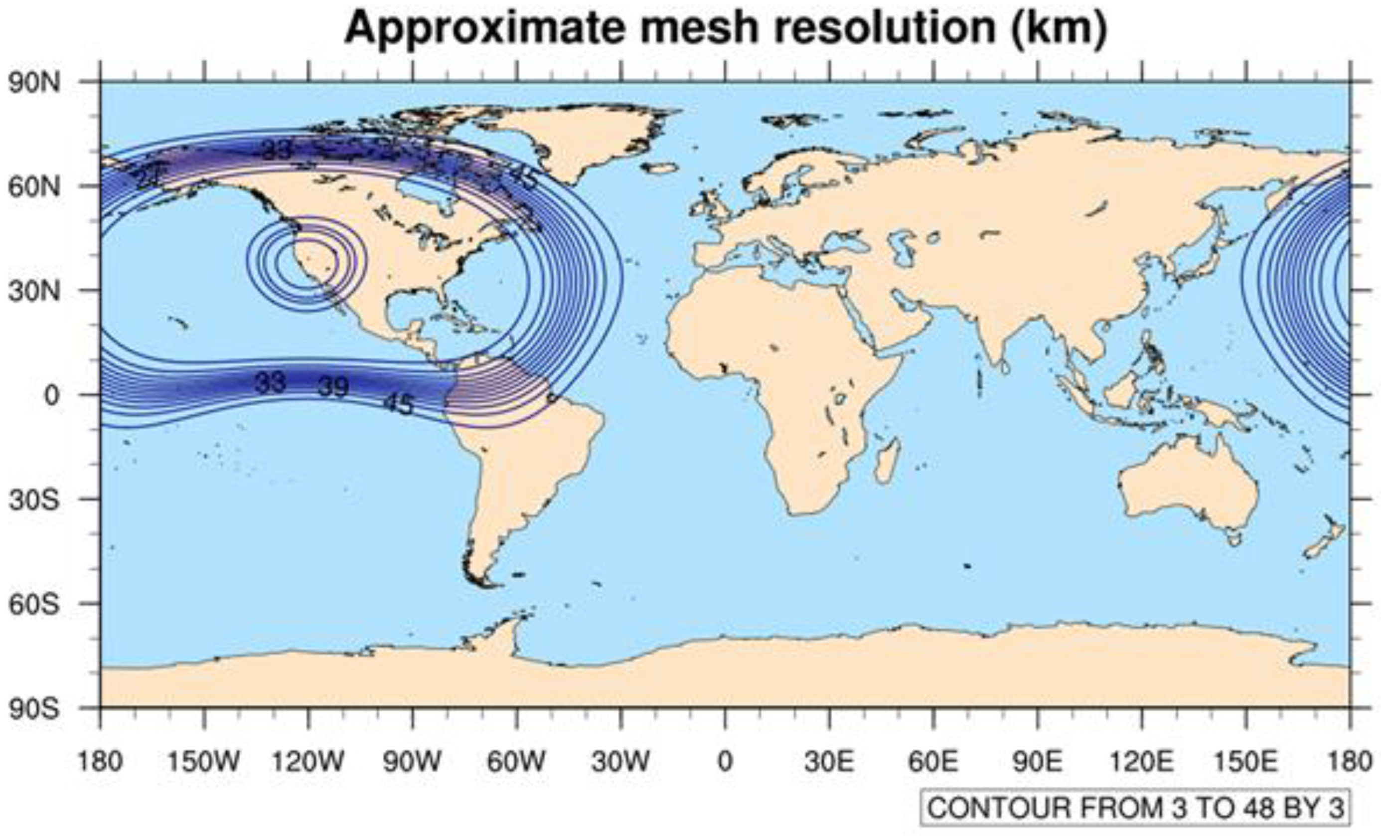
MPAS version 7.0 was used here to simulate atmospheric motions that occurred during the two episodes using a mesh that has variable horizontal grid resolution with hexagonal shapes (Figure S4), which was provided by Michael Duda at NCAR (Michael Duda, personal communication). The spatial resolution of the mesh used in this study ranged from 3 km over California, Nevada, and portions of the neighboring states to steadily increasing to 48 km outwards for the rest of the globe (Figure 2). We did not experiment with the choice of model vertical levels, layer thickness, and model top in MPAS applications as we did not have enough experience with MPAS and adopted the typical values of these choices used by MPAS developers at NCAR. Both regional global applications of MPAS were configured with 55 vertical layers with the first model layer depth corresponding to 20 m and a model top above 25 km. Using our experience at CARB, a WRF model was setup using 30 vertical levels with 30 m deep first layer and with a model top of 15 km. The regional MPAS modeling domain was chosen to be located between 31.8° N and 42.6° N latitudes and 127° W and 112.6° W longitudes as close to the boundaries of 4 km WRF modeling domain used in this study. Model configurations included the NOAH land-surface scheme [24,25], Monin-Obukhov surface layer physics [26,27], YSU boundary layer [28,29], single moment 6-class microphysics [30], and RRTM long- [31] and short-wave radiation parameterizations [32]. WRF simulations are routinely conducted at CARB to use its outputs as an input to air quality models like CMAQ and its model performance is regularly tested against observations (for example, [20]). While the NOAH land surface model was used in both applications of MPAS as it has been widely used by many researchers for its good model performance (for example, [33,34]), the Pleim-Xiu [22,23] land surface model was used in this WRF study since, firstly, MPAS did not have the Pleim-Xiu option available at the time this study was conducted and, secondly, the sensitivity simulations of WRF using several surface physics showed that the Pleim-Xiu option produced a better model performance in WRF as the impact of soil moisture and vegetation is important in predicting the properties of surface layer physics.
Both global and regional applications of MPAS model were initialized using Global Forecast System (GFS) (https://www.ncei.noaa.gov/products/weather-climate-models/global-forecast (accessed on 10 March 2021)) dataset that had 28 km spatial resolution with three hourly intervals. SST data (https://www.nco.ncep.noaa.gov/pmb/products/sst/ (accessed on 10 March 2021)), which also has 28 km spatial resolution but with 12 hourly intervals, were used to update the ocean temperature in MPAS. WRF modeling work that our colleagues performed at CARB [20] was initialized using North American Regional Reanalyses (NARR) (https://rda.ucar.edu/datasets/ds608.0/dataaccess/ (accessed on 10 March 2021)) data that had a 32 km spatial resolution with 3 hourly intervals. WRF SST was updated every 6 h using Global Ocean Data Assimilation Experiment (GODAE) SST data [35]. Chen et al. [20] constructed the WRF modeling domain with three two-way nested grids of 36 × 36, 12 × 12 and 4 × 4 km2 horizontal grid resolutions (Figure S2). The innermost grid (d03) seen in Figure S2 is the area with 4 × 4 km2 resolution in WRF model setup given by Chen et al. [20] that covers California and Nevada. The lateral boundary conditions in WRF [36] are setup by specifying a single row and column and four rows and columns for the relaxation zone along the perimeter of a domain. A coarse grid gives input and boundary conditions to the inner fine grid and the finer grid calculates all atmospheric variables, passes those values back to the parent coarse grid to update all variables within the domain and along the lateral boundaries with no-flux using two-way nested approach. The global application of MPAS does not impose lateral boundary conditions as the modeling domain is one closed sphere while the domain for the regional application of MPAS is taken out of the global domain for the area of interest and lateral boundary condition is created by first relocating the grid points to the nearest Voronoi cell center and constructing a path connecting adjoining cell-center [37] along the perimeter of the regional modeling domain with a variable grid resolution to relax the values of variables along the lateral boundaries. Atmospheric fields are interpolated from the global grid both horizontally and vertically and no-slip or no-flux boundary conditions are used along the lateral boundaries of the regional domain.
We carried out the model performance analysis of both global and regional applications of MPAS over the evaluation domain similar in size to the area used in fine grid WRF domain located between 31.8 °N and 42.6 °N latitudes and 127 °W and 112.6 °W longitudes (Figure S3). However, we did not focus on the model performance of all three modeling applications for the evaluation of temporal evolution of model variables outside of California. Four-dimensional data assimilation (FDDA) in the form of grid nudging or observational nudging (e.g., [36,37,38]) was not available in MPAS at the time this study was carried out and was not used while the WRF simulations utilized grid nudging with surface and upper air data archived at NCAR. NARR, GFS, and SST data were all prepared by WRF Preprocessing System (WPS) that is available from NCAR to initialize both WRF and MPAS models (https://www2.mmm.ucar.edu/wrf/users/download/get_source.html (accessed on 10 March 2021)). Bullock et al. [39] and Judt [39] showed that MPAS errors can build by the 10th day into the simulation and significant differences between observed and predicted model results could be observed, especially in the Polar Regions. Here, we took a more stringent approach to limit the accumulation of modeling errors and each two-week episode was divided into five-day segments with one day spin-up added to the beginning of each segment for all three modeling applications, which is the same approach that was taken by Chen et al. [20] in their WRF simulations.

3. The Data

Meteorological observations of wind, temperature, dew point temperature and pressure collected hourly at 161 surface and upper air observations collected at 00Z and 12Z at three rawinsonde (RAOB) stations located in California for the observations of wind, temperature, dew point temperature and pressure (Figure 1) were used to evaluate the results of both global and regional applications of MPAS and WRF models. The surface and upper air observations collected during the DISCOVER-AQ (NASA, 2013, https://www-air.larc.nasa.gov/missions/discover-aq/discover-aq.html (accessed on 15 February 2021); NOAA, https://ruc.noaa.gov/raobs/ (accessed on 15 February 2021)) and CABOTS [18,19,40] field studies from the Meteorological Assimilation Data Ingest System archive (https://madis.ncep.noaa.gov/ (accessed on 15 February 2021)) were also used to evaluate MPAS results. The observational data were available for the majority of both the winter and summer episodes. Any missing data in both the surface and upper air observational datasets were excluded from the model performance analysis. Observed data points were paired with modeled data points in space and time and statistical calculations, such as MAE, SDEV, RMSE, AC, and BIAS, were carried out using statistical functions in R-library (R-project, https://cran.r-project.org/ (accessed on 10 December 2021), [41] via the mathematical equations (Equations (S1)–(S5) in Supplementary Materials).

4. Results

The guideline for the performance evaluation of WRF model is discussed by the EPA [42] as that approach was applied here to evaluate the performance of all three models in capturing the observed meteorological conditions. The results of the model performance evaluations shown here are: (a) averaged values of the horizontal cross section of the 10 m wind speed and direction, 2 m temperature, 2 m mixing ratio, 2 m relative humidity and planetary boundary layer height (PBLH) predicted by the models to study their spatial and temporal distributions over California; (b) the temporal evolution of the characteristic meteorological variables during each episode along with their corresponding statistical quantities calculated during each episode to evaluate the diurnal changes of 2 m temperature, 2 m mixing ratio, 2 m relative humidity, and 10 m wind speed and direction along with the quantitative values of model agreement with the observations as well as the modeling errors; (c) the average diurnal changes of BIAS, MAE, and SDEV calculated over California to investigate diurnal variability in the model errors and deviation from their respective mean predictions; (d) the comparisons of model estimates of temperature, dew point temperature and wind speed and direction predictions in the vertical against observations at rawinsonde stations in California, and (e) the spatial distribution of AC and BIAS statistics for 2 m temperature and 2 m mixing ratio to find out where over California each model performs well using AC values and how much of an error each model commits in predicting temperature and mixing ratio using BIAS values.

4.1. Comparison to Observations—January 2013 Winter Episode

4.1.1. Average Horizontal Spatial Distribution

Horizontal spatial distribution of 10 m wind flow, 2 m air temperature, 2 m water vapor mixing ratio, 2 m relative humidity and PBL height predicted by all three models were studied to evaluate how each model represents the evolution of these typical atmospheric variables in space and time. However, since meteorological conditions can vary greatly from one hour to the next, it is difficult to evaluate model results using hour-by-hour model fields. Therefore, we present the averages of characteristic variables calculated at 8 AM and 2 PM local time here to demonstrate the general ability of each model in simulating meteorological conditions in the morning and the afternoon hours, respectively. Since the meteorological observations of characteristic variables are not available at all grid points over the evaluation domain, and interpolation of available surface observations to nearby grid points where there is no observational data may not necessarily represent those grid points, we could not perform a direct comparison of model results at grid points locations where there is no observation, or the observation point is too far to a grid point. Therefore, the averaged model results presented here intend to give a sense of each model’s ability to predict the variables in an average sense. The model results will be compared to the hourly observations at surface stations over the two-week period and in the vertical at specified times by interpolating the model predicted values to the location of observation point using inverse distance weighted average method to assess their ability to predict the observed conditions.
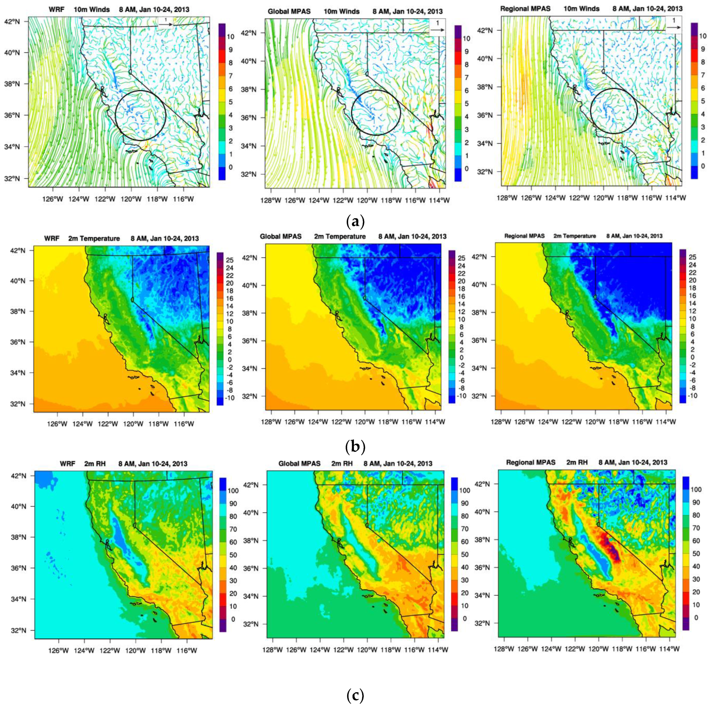
The atmospheric wind flow depicted by 10 m wind vectors averaged at 8 AM during the winter episode show that all three models predict the general direction of atmospheric flow that are typically observed along the valley, over elevated terrain, and off the coast of California (Figure 3a) reasonably well. More specifically, all three models prognose the occurrence of downslope winds due to cold drainage flow that takes place from evening to early morning hours, combined with a downwind flow within valley floor, as shown in the figure using a symbol between a vector and a streamline representation of wind flow. In addition, land breeze along the coast from inland towards Pacific Ocean near San Francisco Bay and Los Angeles basin at early morning hours is also observed (Figure 3a). Furthermore, when the conditions are right, a local circulation called the Fresno Eddy around Fresno in central San Joaquin Valley forms at night and early morning hours [43,44]. All three models predict the existence of this local circulation (highlighted by a circle in each frame). Fresno Eddy is characterized by recirculating air masses that can keep the local air mass over the same area for prolonged period that can lead to elevated pollution levels [45] (Figure 3a). The afternoon winds at 2 PM are seen giving rise to upslope winds both towards the Sierra Nevada mountains from the valley floor to the east and towards the Cascades along the west coast (Figure S10). Furthermore, all three models predict a sea breeze circulation forming along the coast during the day, especially over Santa Barbara and Los Angeles area while the sea breeze circulation in northern California starting from San Francisco Bay area is predicted to be more pronounced (Figure S10).
The average 2 m air temperature at 8 AM shows that a cooler air mass lies within the Central Valley, which is surrounded by slightly warmer temperatures along the foothills while the air temperature is colder (0 °C or lower) at higher elevations over Sierra-Nevada mountains, and warmer (around 10 °C) along the coast in Southern California between Los Angeles and San Diego (Figure 3b). Afternoon 2 m temperature within the central valley rises to about 10 °C during the day while it rises to about 20 °C in the Los Angeles basin (Figure S11). Along with the near surface cooling early in the morning (Figure 3b) and warming in the afternoon (Figure S11), 2 m water vapor mixing ratio values increase during the day from morning (Figure S12) to afternoon (Figure S13) due to evaporation near the surface as this is particularly noticeable within the SV-SJV corridor (Figures S12 and S13). While 2 m mixing ratio values within SV and SJV increase in the afternoon, the increase of temperature in time causes the relative humidity values to drop from 80% in the morning (Figure 3c) to about 30% in the afternoon (Figure S14). Average Planetary Boundary Layer Heights (PBLH) predicted by all three models are below 100 m at early morning hours, especially along the Central Valley corridor (Figure S15) while they increase to a range between 500 and 700 m in the afternoon (Figure S16). Since the observations of PBLH values are scarce, we did not analyze how the average PBLH values predicted by MPAS compare against the PBLH observations, as many factors, such as the prevalent weather conditions like a strong high pressure system, downwind transport of large air masses from one region to another and inversion and stagnation play a major role in determining the PBLH values.

4.1.2. Time Series at Surface Stations

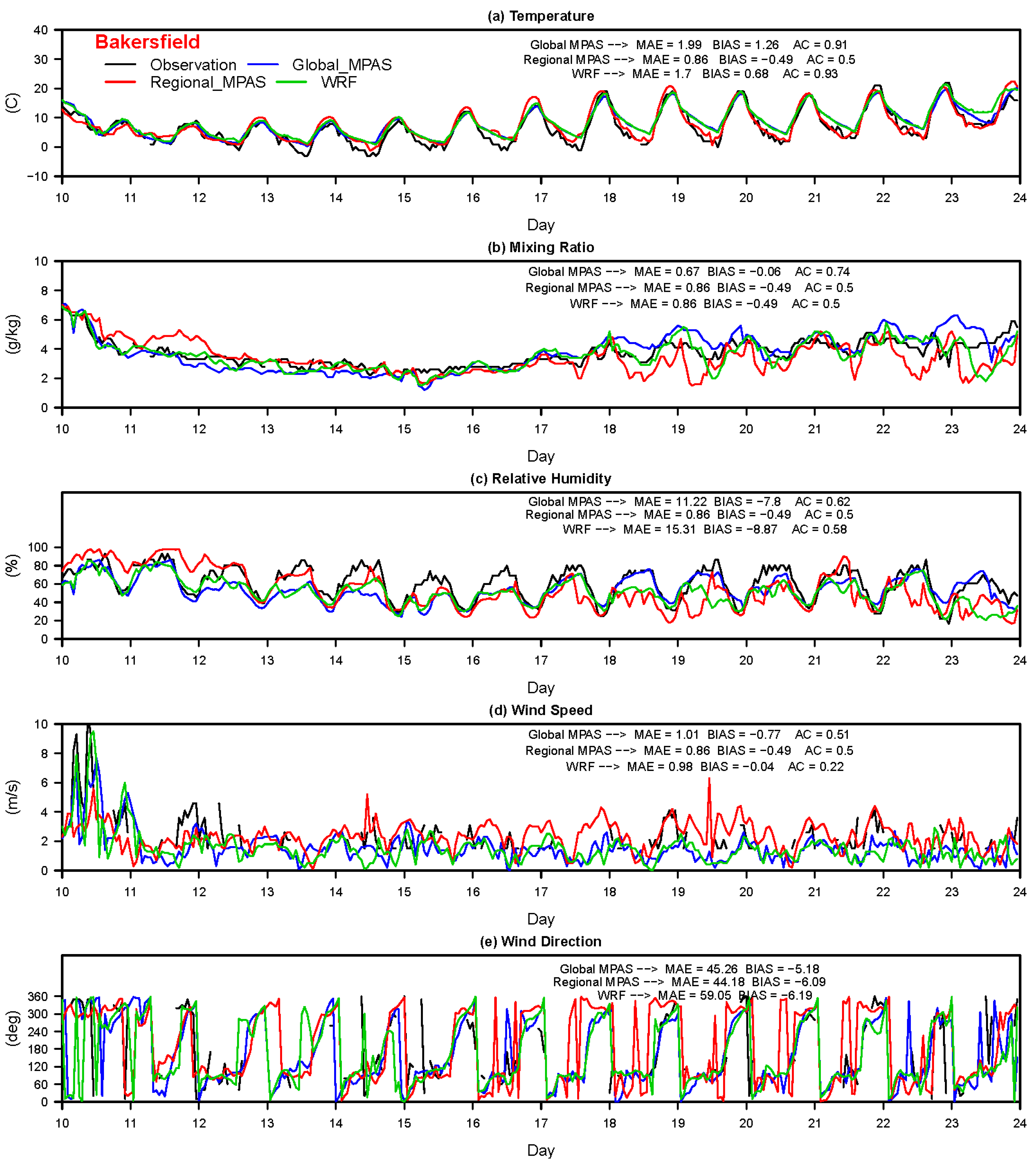
Among 161 surface stations, Modesto, Fresno, Visalia, and Bakersfield stations from SJV, Sacramento from SV, Oakland from SFB, Los Angeles from South Coast (SC), and San Diego from San Diego air basin were chosen to show the performance of all three models. The complex interactions between the ocean–land interface, orographically induced flows from the mountain-valley topography, and the extreme temperature gradients between the ocean, delta region, valley floor, and mountain ranges surrounding the valley, make the SJV one of the most challenging areas in the country to simulate using prognostic meteorological models. Therefore, four surface stations located in the north, central and south of the valley were chosen from the SJV to show the model performance compared to one station from the other air basins chosen. Hourly variations of the predicted values of 2 m temperature, 2 m water vapor mixing ratio, 2 m relative humidity, and 10 m wind speed and direction against observations at Bakersfield in SJV over the two-week winter 2013 episode are given in Figure 4. The comparison of the same meteorological parameters at other stations are given in the Supplementary Materials (Figures S17–S23), respectively. All three models predict the diurnal variation of all five characteristic atmospheric variables reasonably well at Bakersfield (Figure 4). However, some differences of model performance among three models against observations are also seen. For example, while all three models generally capture the maximum temperature on each day, global MPAS and WRF underestimate the nighttime minimum temperature on some days at Bakersfield as regional MPAS predicts the nighttime minimum temperature better. A good prediction of daily maximum temperatures by all three models and underprediction of nighttime temperatures by global MPAS and WRF while a better prediction of nighttime temperatures by regional MPAS is also seen at Fresno (Figure S17), Sacramento (Figure S18), Modesto (Figure S19), Oakland (Figure S20), and San Diego (Figure S23). On the other hand, the nighttime minimum temperature is underestimated by regional MPAS while global MPAS and WRF capture it well at Los Angeles (Figure S21) and Visalia (Figure S22).
The diurnal evolution of mixing ratio and relative humidity are also predicted well by global MPAS and WRF while regional MPAS underpredicts both variables at Bakersfield (Figure 4) on some days and overpredicts the daily maximum relative humidity at Fresno (Figure S17), Sacramento (Figure S18), Modesto (Figure S19), Visalia (Figure S22), and San Diego (Figure S23). However, regional MPAS captures the diurnal evolution of 2 m mixing ratio and relative humidity well at Oakland (Figure S20) while global MPAS and WRF underestimate both. We do not know why the regional MPAS can predict the diurnal variation of the mixing ratio and relative humidity better at Oakland while global MPAS and WRF cannot. We first speculate that this might have to do with Oakland being a coastal station where the magnitude of the diurnal variation of moisture and temperature is smaller than those at inland stations and this might cause model error build-up being smaller at such stations. However, this does not quite explain why the regional MPAS does a better job in predicting the evolution of mixing ratio and relative humidity at Oakland while global MPAS does not even though they both have the same physics. On the other hand, Los Angeles and San Diego, as other coastal stations in the Supplementary Materials, indicate a good prediction of the mixing ratio and relative humidity for all three applications compared to the better prediction of the regional application at Oakland.
Additionally, the evaluation of the diurnal evolution of wind speed and direction during the episode does not show too much a difference among all three model applications compared to the observations at all sites (Figure 4 and Figures S17–S23). It should be noted that some wind observations at some hours are missing at some sites. When the statistical metrics (MAE, BIAS, and AC) are used to study model performance (see those values given on the right side of each frame plotted for each model variable), AC values of wind speed for all three models are 0.5 or lower (Figure 4 and Figures S17–S23) at all stations shown except at San Diego where it varies between 0.72 and 0.83, while MAE and BIAS vary from one station to the next. Yet, the magnitudes of these statistical metrics are not too far apart for each model. AC values of all three models for temperature are mostly in the 0.8–0.9 range at all stations except it is 0.5 for regional MPAS at Bakersfield (Figure 4). Similarly, AC values of 2 m mixing ratio and 2 m relative humidity for all three models are also high with values ranging from 0.5 to 0.9. One of the key results that can be withdrawn from this statistical analysis of 2 m temperature, 2 m mixing ratio, 2 m relative humidity, 10 m wind speed and direction for this winter episode is that the agreement of all three models’ prediction of the characteristic variables used here with observed values are high via high AC values with observations, and similar magnitude of MAE and BIAS error values against observations at most stations examined here.

4.1.3. Diurnal Statistics

In addition to the comparisons of the temporal evolution of characteristic atmospheric variables predicted by each model against observations during the two-week 2013 winter episode (for example, Figure 4), BIAS, MAE, and SDEV values of 2 m temperature and 2 m mixing ratio generated by each model at each hour at all 161 stations located in the evaluation domain during the two-week episode were averaged over 24-h period to evaluate how much of an error each model commits in predicting these two variables and how much 2 m temperature and 2 m mixing ratio values deviate from their mean values. The average daily variation of BIAS, MAE, and SDEV of 2 m temperature and 2 m mixing ratio are given in Figure 5. The BIAS for 2 m surface temperature (Figure 5a) shows a gradual increase from −1 °C in the evening at 01 UTC (5 PM local time) for both global and regional MPAS to 2 °C at 16 UTC (8 AM local time) for global MPAS and 2.5 °C for regional MPAS at the same hours. On the other hand, diurnal temperature BIAS for WRF changes from −0.5 °C at 01 UTC (5 PM local time) to 2 °C at 15 UTC (7 AM local time). In addition, all three models show a similar diurnal error variation for 2 m temperature in an average sense. While all three models generate nearly the same magnitude of temperature BIAS (Figure 5a) during the day, the maximum temperature error occurs one hour earlier for WRF than the timing for both global and regional MPAS temperature error. In addition, MAE of near surface temperature varies between 2 and 3 °C while SDEV varies between 3 and 4 °C diurnally for global and regional MPAS and 2.5 to 3.5 °C for WRF (Figure 5c). Similarly, 2 m water vapor mixing ratio BIAS varies between 0.25 and −0.25 g/kg for global and regional MPAS and within 0.75 g/kg for WRF (Figure 5d). At the same time, MAE is less than 1 g/kg for all three models, and SDEV is less than 1.5 g/kg for all three models (Figure 5e). Furthermore, regional MPAS appears to commit a smaller MAE error for 2 m mixing ratio than global MPAS and WRF models for the winter episode. Finally, the variation of SDEV from its mean value for 2 m mixing ratio is smaller for WRF with average values around 1 g/kg than both global and regional MPAS with average values 1.25 g/kg (Figure 5f). The diurnal variation of RMSE in terms of its tendency over spatially averaged values over the modeling domain and its magnitude for various variables was not too different than those of SDEV (see Figures S71–S74 to compare against Figure 5 and Figure 9). As we show BIAS, MAE and SDEV statistics to evaluate the agreement of modeling applications with the observations and errors that each application commit in predicting various quantities in Figure 5 for winter and Figure 9 for summer, we provide RMSE and the comparison of its systematic and unsystematic components against RMSE for temperature and mixing ratio by Figures S71 through S74 in the Supplementary Materials.

4.1.4. Rawinsonde Measurements

As opposed to surface measurements obtained at many sites, upper air rawinsonde measurements are generally very sparse, but available upper air data provide an additional way to assess overall model performance. To evaluate the upper air predictions of all three models, rawinsonde observations collected at Oakland airport, Miramar Air Force Base (AFB) and Vandenberg AFB between 10 and 23 January 2013 0Z were retrieved from the NOAA rawinsonde observation database (https://ruc.noaa.gov/raobs/ (accessed on 15 February 2021)). The vertical structure of temperature, dew point temperature and wind speed and direction predicted by all three models were plotted within individual frames for a better comparison against observed conditions at Oakland (Figure 6), Miramar Air Force Base (AFB) (Figure S24), and Vandenberg AFB (Figure S25) on 15 January, 00Z. All three models generally capture the observed conditions relatively well. Specifically, they each capture the elevated inversion layer seen at about 850 mb that is identified by an increasing temperature with height, and then decreasing temperature with height starting around 700 mb, and the increasing temperature at tropopause around 200 mb for Oakland station (Figure 6). The observed wind direction with height is also captured well by all three models while the magnitude of the observed wind with height is underestimated by all three models. Additional comparisons of rawinsonde plots against observations at Miramar AFB (Figure S24) and Vandenberg AFB (Figure S25) given in the Supplementary Materials point out a good agreement of temperature and dew point temperature predictions and underestimation of the wind with height at both stations.

4.2. Comparison to Observations—July 2016 Summer Episode

4.2.1. Average Horizontal Spatial Distribution

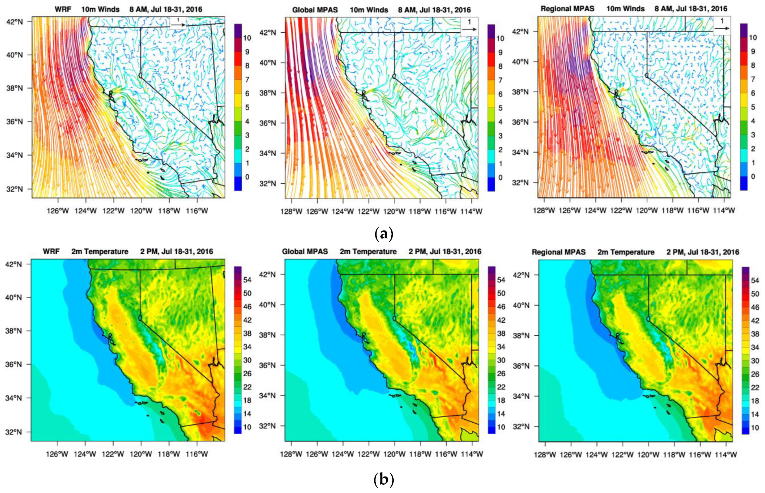
Like the winter episode, atmospheric flow depicted by 10 m wind speed and direction, 2 m temperature, 2 m water vapor mixing ratio, 2 m relative humidity and PBLH predictions were averaged at 8 AM and 2 PM to provide an averaged behavior of models’ predictions of the characteristic variables for the summer episode. The 10 m wind vectors at 8 AM show (Figure 7a) that downslope winds that were seen in winter episode at 8 AM are not seen during summer mornings, and there is now an upslope flow from the valley flow towards higher elevations already in progress due to the increasing solar radiation as sunrise starts impacting the near surface temperature at around 6 AM. In addition, the marine layer is seen to penetrate inland along the entire coast but is especially strong in the San Francisco Bay region and Los Angeles basin (Figure 7a). Furthermore, the marine air enters the Sacramento Valley and splits into northern and southern branches while the southern branch is more pronounced. The marine inflow from San Francisco Bay area gets stronger in the afternoon and sea breeze circulation is seen to dominate the valley floor winds (Figure S30). Moreover, the sea breeze is particularly strong in San Francisco Bay region in Northern California and Los Angeles basin in Southern California. It is a common occurrence of air near surface warming up rapidly in the afternoon during summer in the central California and especially in southern San Joaquin Valley (Figure S31) as higher elevations surrounding the central valley prevent the downwind transport of atmosphere. While 2 m water vapor mixing ratio does not significantly decrease from morning (Figure S32) to the afternoon (Figure S33) as a response to increasing temperatures in time (Figure S31), 2 m relative humidity is first predicted to be around 60% in SV in the morning (Figure 7c) and decreases rapidly to 20% during the day (Figure S34), as predicted by all three models. Finally, the average PBLH values within the Central Valley are estimated to be less than 300 m (Figure S35) in the morning while they get deeper with values less than 1500 m in the afternoon with shallower pockets along the Central Valley (Figure S36). Furthermore, the average PBLH predicted by the regional MPAS in the regional modeling domain is less than those predicted by WRF and global MPAS (Figure S35).

4.2.2. Time Series at Surface Stations

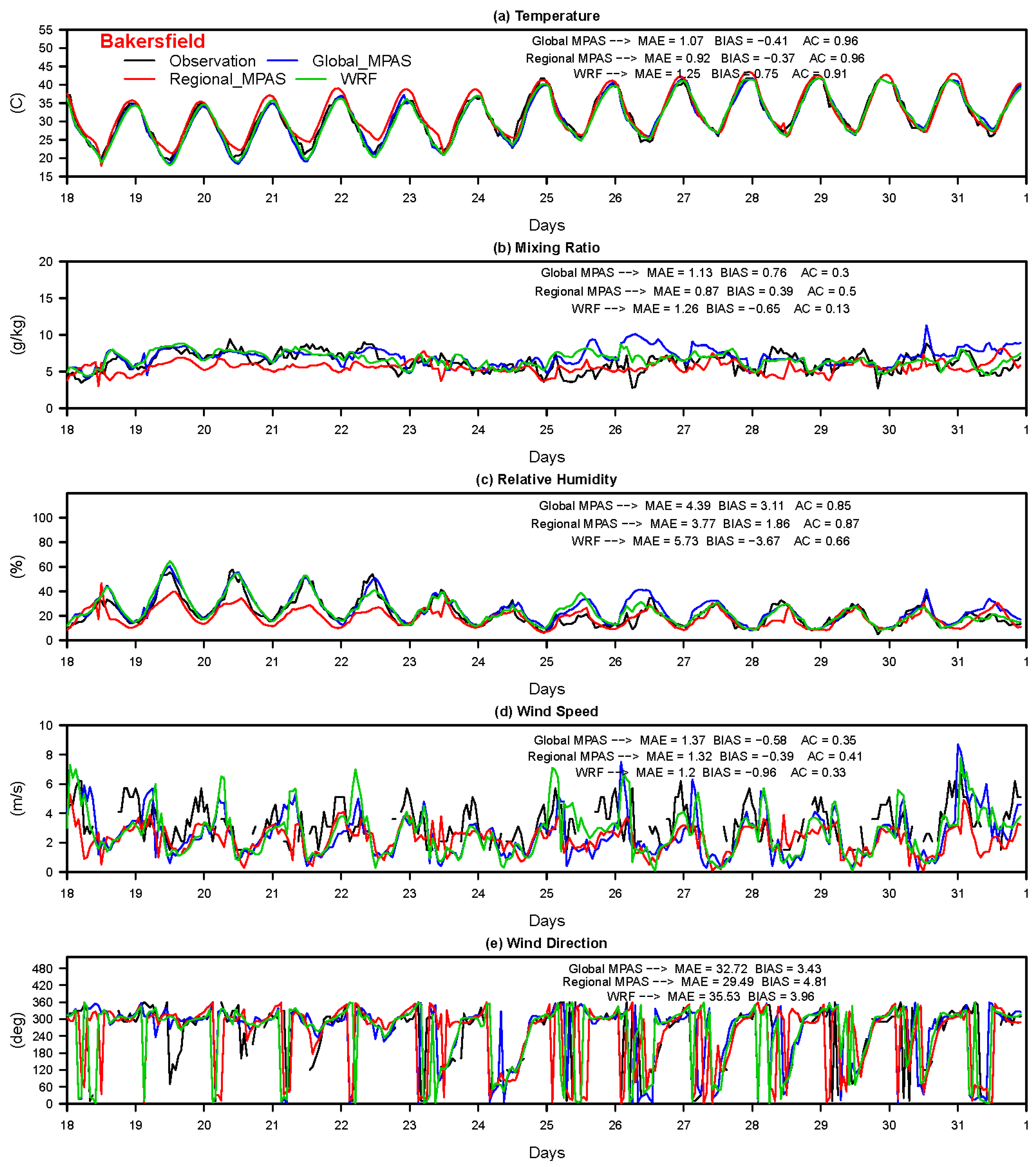
Similar to the 2013 winter episode, time series analyses for 2 m temperature, 2 m water vapor mixing ratio, 2 m relative humidity, 10 m wind speed and direction predicted by all three models against surface observations during the two-week summer 2016 episode are given at Bakersfield (Figure 8) while figures for Fresno, Sacramento, Modesto, Oakland, Los Angeles, Visalia, and San Diego stations are given in Figures S37–S43, respectively, in the Supplementary Materials. The comparisons of time series analysis in Figure 5 for winter 2013 and in Figure 8 for summer 2016 episodes at Bakersfield indicate that all three models predict 2 m temperature at Bakersfield slightly better in summer (Figure 8) than in winter (Figure 5). In particular, the nighttime underprediction of temperature seen in winter by each model on different days decreases in summer although a slight overestimation of daytime maximum temperature at Bakersfield is still seen for regional MPAS. Furthermore, the improved model performance for temperature during summer at Bakersfield is also supported by a slightly higher AC and smaller MAE and BIAS values calculated during summer (Figure 8) than during winter at Bakersfield. Similarly, 2 m mixing ratio and 2 m relative humidity are also predicted well by all three models while regional MPAS slightly underpredicts 2 m relative humidity at Bakersfield (Figure 8), Fresno (Figure S37), Sacramento (Figure S38), and Visalia (Figure S42) on some days during the summer as 2 m mixing ratio is predicted reasonably well by all three models.
When higher values of AC correlation with observations, and lower values of MAE and BIAS errors away from the observations are taken into account to evaluate each model’s performances in predicting the characteristic atmospheric variables, all three statistical metrics indicate that all three models predict 2 m temperature and 2 m relative humidity slightly better in summer than in winter. This is seen at Bakersfield (Figure 4 vs. Figure 8), Fresno (Figure S17 vs. S37), Sacramento (Figures S18 vs. S38), Modesto (Figures S19 vs. S39), Oakland (Figures S20 vs. S40), Los Angeles (Figures S21 vs. S41). On the other hand, the performance of all three models in predicting 2 m mixing ratio shows a slight decrease at all these stations through a lower AC and higher MAE and BIAS values in summer than in winter while all three models show a better prediction in summer than in winter via higher AC values and lower MAE and BIAS error at Visalia (Figures S22 vs. S42) and San Diego (Figures S23 vs. S43). The day-to-day variation of wind speed and wind direction are also predicted reasonably well at nearly all stations except at Oakland (Figure S40) where peak wind speed is underpredicted by all three models.

4.2.3. Diurnal Statistics

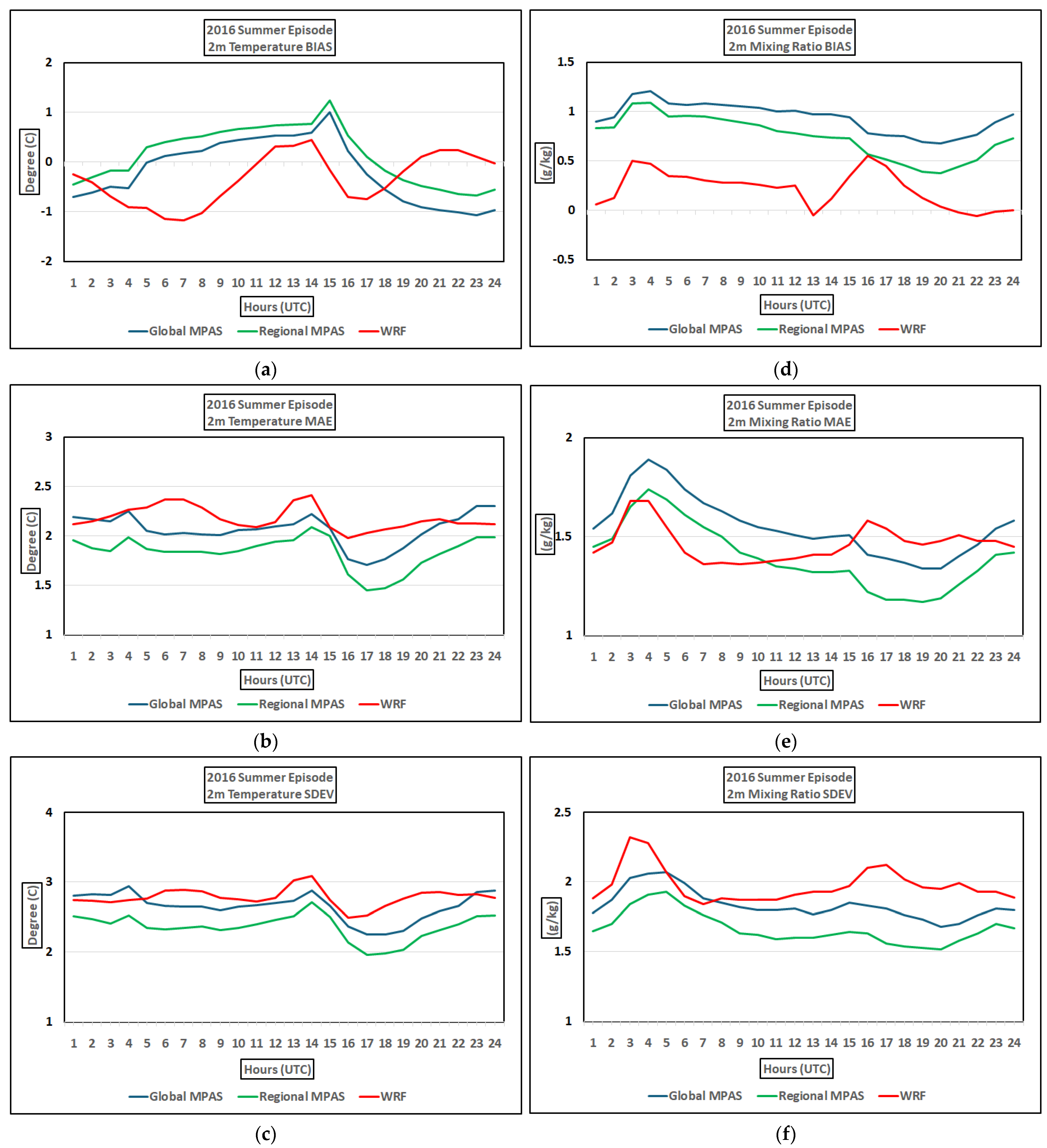
The average diurnal variation of 2 m temperature BIAS committed by global MPAS and regional MPAS are very similar to each other in terms of its magnitude and shape of the error tendency (Figure 9a). The 2 m temperature BIAS first increases in time until it reaches a maximum value by midday and then decreases for the rest of the day for global and regional MPAS. On the other hand, the 2 m temperature BIAS for WRF shows an undulating tendency with decreasing and increasing values during the day (Figure 9a). The magnitude of temperature BIAS varies between −0.75 and 1 °C for global MPAS, between −0.5 and 1.2 °C for regional MPAS, and between −1.2 and 0.3 °C for WRF model. The time for the occurrence of maximum temperature BIAS is at 15 UTC (7 AM local time) for both global and regional MPAS and 14 UTC (6 AM local time) for WRF model. Furthermore, BIAS for WRF shows two temperature minima, one at 7 UTC (11 PM local time) and the other at 17 UTC (9 AM local time), and two temperature maxima, one at 14 UTC (6 AM local time) and the other at 21 UTC (1 PM local time) as the BIAS error is mostly negative during the day. Compared to this, the BIAS error for global and regional MPAS is positive between 4 and 5 UTC (10–11 PM local time), and between 16 and 17 UTC (10–11 AM local time), and negative at other times during the day. The magnitudes of MAE (Figure 9b) of 2 m temperature are less than 2.4 °C and that of SDEV (Figure 9c) are less than 3 °C for all three models. Additionally, the shape of daily tendencies for the variation of MAE and SDEV show are very similar to each other noting that there is not much a discrepancy among three models for the magnitudes of MAE and SDEV for 2 m temperature. The magnitude of 2 m mixing ratio BIAS is less than 1.25 g/kg for both global and regional MPAS while that of WRF is less than 0.5 g/kg as the BIAS error is mostly positive for all three models (Figure 9d). The general tendency of the diurnal variation of MAE (Figure 9e) and SDEV (Figure 9f) are very similar to each other for all three models with a decrease of error later in the evening and then decreasing with time. Additionally, the magnitudes of both MAE and SDEV are less than 2 g/kg for all three models.

4.2.4. Rawinsonde Measurements

Like the winter episode, the rawinsonde data collected at Oakland airport, Edwards AFB, and Vandenberg AFB between 18 July 2016, 0Z and 31 July 2016, 0Z were retrieved from NOAA (https://ruc.noaa.gov/raobs/ (accessed on 1 February 2021)). The comparisons of model predictions with the observed vertical profile on 20 July 2016, 12Z show that all three models capture the shallow inversion layer that formed near the surface as well as the general structure of temperature with height. In addition, the change of wind direction with height is also captured well although the magnitude of the wind direction and its change with height is underestimated by all three models. The observed vertical profile of dew point temperature indicates that the atmosphere was composed of juxtaposition of several dry and somewhat more moist layers vertically. While the overall shape of the dew point temperature profile predicted by each model are very similar to each other and all three models predict the average dew point temperature profile, they cannot predict the variation of dew point temperature properly (Figure 10). A reasonably good prediction of observed temperature with height is also seen at Vandenberg AFB (Figure S44) and Miramar AFB (Figure S45) stations, while the dew point temperatures and the magnitude of the wind direction are not captured accurately by any model as the general shapes of temperature, dew point temperature and wind direction with height are very similar to each other.

5. Summary and Conclusions

Meteorological models are regularly tested over different regions and over multiple seasons under a variety of surface conditions and prevalent weather systems impacting the area of interest to determine if they can be used to analyze the observed atmospheric conditions and to predict future atmospheric conditions as a reliable forecasting tool. Given that MPAS is a relatively new model, it is important to evaluate the strength and weakness of MPAS model in reproducing the atmospheric conditions. Large scale weather systems affecting the west of the US typically originate over the Pacific Ocean, move over California, and interact with the complex terrain, and show large variations from winter to summer. It is also a good idea to seek and numerically simulate a time period that is important to study the meteorological conditions for various reasons. Therefore, a two-week winter episode, 10–24 January 2013, during the DISCOVER-AQ field campaign conducted to study PM and another two-week summer episode, 18–31 July 2016, during the CABOTS field campaign conducted to study O3 were selected to evaluate MPAS model performance over California.
A comprehensive model performance evaluation of global and regional versions of MPAS and WRF models was carried out using 2 m temperature, 2 m mixing ratio, 2 m relative humidity, 10 m wind speed and direction, as well as the PBL height values. First, the horizontal cross sections of these variables that are averaged at 8 AM and 2 PM local time were analyzed to evaluate how these three models represent the temporal evolution and the spatial distribution of these variables in the morning and the afternoon in an average sense. Then, temporal evolution of 2 m temperature, 2 m mixing ratio, 2 m relative humidity, 10 m wind speed and direction predicted by all three models during two-week winter and summer episodes were compared against observations collected at 161 surface stations while only the results of a select stations were shown in this study. In addition, the vertical profiles of temperature, dew point temperature, wind speed and direction predicted by all three models were compared to the vertical profiles observed at 3 rawinsonde stations. Model performance statistics, including AC, RMSE, MAE, BIAS, and SDEV for 2 m surface temperature, 2 m water vapor mixing ratio, 10 m wind speed and direction were also calculated to further evaluate the ability of all three models in reproducing the observed meteorology.
As pointed out by the synoptic conditions examined for the winter and summer episodes studied here (see Supplementary Materials), large-scale high-pressure systems that typically form over California with varying magnitudes of surface pressures are associated with stagnant conditions and can lead to elevated air pollution episodes within central California, especially in SV and SJV. The plots of wind flow averaged at 8 AM and 2 PM show that all three models predicted the characteristic atmospheric flow that occur in California, such as the upslope flow from the valley floor to higher elevations, downslope flow from elevated terrain into the valley, the downwind flow along the valley floor, intrusion of marine air into inland from Pacific Ocean typically as sea breeze during the day or later in the afternoon, as well as land breeze at night. A rarely noticed phenomenon known as Fresno Eddy was also predicted to occur in Fresno area in SJV by all three models. The plots for the temporal evolution of 2 m temperature during winter and summer episodes at surface stations throughout domain show that observed nighttime temperature minima and daytime maxima are predicted reasonably well by all three models in both winter and summer. The agreement between the predictions and the observations are somewhat better in summer than in winter for all three models with slightly higher AC correlations and smaller error values. However, some differences are also seen between each models’ predictions of temperature. For example, the global MPAS and WRF underestimate the nighttime minimum temperature on some days while regional MPAS predicts the nighttime minimum temperature better on those days while the daytime maximum temperatures are typically well predicted by all three models. The diurnal evolution of 2 m mixing ratio and 2 m relative humidity are predicted well by global MPAS and WRF while regional MPAS underpredicts both variables at some stations and days and overpredicts the daily maximum relative humidity on some days. Furthermore, the predictions of 10 m wind speed and direction do not show too much a difference from one model to the next as wind speed predicted reasonably while wind direction estimates can show a larger variation for all three models.
The diurnal variation of domain-wide averaged BIAS and MAE statistical metrics for 2 m temperature and 2 m water vapor mixing ratio calculated from all three models indicate that the magnitudes of these error statistics are small with a maximum of 2 °C bias for temperature in winter and 1 °C in summer while the magnitudes of 2 m mixing ratio bias are ±0.5 in winter and less than 1 g/kg in summer as SDEV is slightly larger than these values. In addition, AC values against observations are high for characteristic meteorological variables. On the other hand, RMSE values are slightly larger with values around 3–3.5 °C in winter (Figure S71a) and 2.5–3 °C (Figure S73a) in summer for temperature while those for the mixing ratio varies between 1 and 1.5 g/kg in winter (Figure S72a) and around 2 g/kg (Figure S74a) in the summer. In addition to these statistics, we also looked at the systematic and unsystematic components of RMSE for temperature and mixing ratio to see what percentage of RMSE error is coming from each component. Figures S72–S74 show that major portions of the RMSE error for both temperature and mixing ratio is stemming from systematic component although still a considerable portion of RMSE is also coming from unsystematic portion of RMSE.
The spatial distribution of AC and BIAS values (see Supplementary Materials for detailed discussion) were plotted for 2 m temperature, 2 m mixing ratio, and 10 m wind speed and direction for both winter and summer episodes show that all three models perform well in predicting the observed temperature through a high AC skill score. On the other hand, both global and regional MPAS have a negative BIAS of about 2 °C at some stations in northern California, at elevated terrain and along San Francisco-Sacramento corridor. The reason for the poorer model performance at some stations needs to be investigated in future applications using various different physics option through sensitivity studies. In short, the spatial AC and BIAS plots point out that the AC agreement of model predictions with the observations and the modeling errors are similar in magnitude to each other or are not substantially different from each other for all three models although some differences are still seen at different parts of the evaluation domain. Typically, AC values in predicting 2 m temperature are high for each model and BIAS errors are not too large from each other. However, the spatial distribution of AC values in predicting 2 m mixing ratio are smaller than those for 2 m temperature. Furthermore, AC values vary from 0.3 to 0.8 in predicting 10 m wind speed and 0.1 to 0.8 in predicting 10 m wind direction for all three models during both winter and summer episodes.
Overall, the evaluation of global and regional applications of MPAS model against observations and WRF model results show that both global and regional MPAS modeling applications predict the characteristic meteorological variables reasonably well and as well as WRF model does. While there are some areas over the evaluation domain and some days where each model underperforms in predicting the observed conditions, all three model results are comparable to each other. The magnitudes and the behavior of the diurnal variation in error statistics will likely change when different model physics are used, as well as the time periods chosen. Sensitivity studies to measure these variations in future studies would give further information on the ability of global and regional applications of MPAS model to capture observed conditions under different time and weather conditions over California. The magnitudes of RMSE, MAE and BIAS errors for all characteristic variables are expected to decrease with the use of nudging options in MPAS as the model will be pushed towards observed conditions. Overall, this study demonstrates that both global and regional versions of MPAS predict the observed meteorological conditions over California reasonably well and their results are comparable to those of WRF. In addition, as MPAS is further developed to include more advanced options, such as observational nudging, these options should be tested, and model performance should be reassessed. The use of other available parameterization schemes as part of sensitivity studies should also help further in selecting model modules that would produce more reliable model options.

Supplementary Materials

The following supporting information can be downloaded at: https://www.mdpi.com/article/10.3390/atmos15101248/s1. References [46,47,48,49,50,51,52,53,54,55,56,57] are cited in Supplementary Materials.

Author Contributions

Conceptualization, K.G., C.C. and J.C.A.; methodology, K.G.; software, K.G.; validation, K.G.; formal analysis, K.G.; investigation, K.G.; resources, K.G.; data curation, K.G.; writing—original draft preparation, K.G.; writing—review and editing, K.G., Z.Z., C.C. and J.C.A.; visualization, K.G.; supervision, C.C. and J.C.A.; project administration, J.C.A.; funding acquisition, J.C.A. All authors have read and agreed to the published version of the manuscript.

Funding

This research received no external funding.

Institutional Review Board Statement

Not applicable.

Informed Consent Statement

Not applicable.

Data Availability Statement

The data used to initialize and run MPAS model in this work are publicly available for global gridded analysis data from NOAA-GFS (https://www.ncdc.noaa.gov/data-access/model-data/model-datasets/global-forcast-system-gfs (accessed on 10 March 2021)), for additional gridded analysis, surface, and upper air data from NCAR (https://rda.ucar.edu/ (accessed on 10 March 2021)), for sea-surface temperature data from NCEP (https://www.nco.ncep.noaa.gov/pmb/products/sst/ (accessed on 10 March 2021)), and for upper air RAOB data from NOAA (https://ruc.noaa.gov/raobs/ (accessed on 10 March 2021)). MPAS model results are also available from authors upon request.

Acknowledgments

We are grateful to Michael Duda at the National Center for Atmospheric Research (NCAR) located at Boulder, Colorado, for his technical support for this study. We are also grateful to Robert Gilliam at the Environmental Protection Agency (EPA) who helped us to analyze the data properly.

Conflicts of Interest

The authors declare no conflict of interest. This paper has been reviewed by the staff of the California Air Resources Board and has been approved for publication. Approval does not signify that the contents necessarily reflect the views and policies of the California Air Resources Board, nor does the mention of trade names or commercial products constitute endorsement or recommendation for use.

References

  1. Avissar, R.; Pielke, R.A. A Parameterization of Heterogeneous Land Surfaces for Atmospheric Numerical Models and Its Impact on Regional Meteorology. Mon. Wea. Rev. 1989, 117, 2113–2136. [Google Scholar] [CrossRef]
  2. Mahrer, Y.; Pielke, R.A. The Effect of Topography on Sea and Lan Breezes in a Two-Dimensional Numerical Model. Mon. Wea. Rev. 1977, 105, 1151–1162. [Google Scholar] [CrossRef]
  3. Giovanni, L.; Ferrero, E.; Karl, T.; Rotach, M.W.; Staquet, C.; Castelli, S.T.; Zardi, D. Atmospheric Pollutant Dispersion over Complex Terrain: Challenges and Needs for Improving Air Quality Measurements and Modeling. Atmosphere 2020, 11, 646. [Google Scholar] [CrossRef]
  4. Lehner, M.; Rotach, M.W. Current Challenges in Understanding and Predicting Transport and Exchange in the Atmosphere over Mountainous Terrain. Atmosphere 2018, 9, 276. [Google Scholar] [CrossRef]
  5. Klemp, J.B.; Skamarock, W.C.; Fuhrer, O. Numerical consistency of metric terms in terrain-following coordinates. Mon. Wea. Rev. 2003, 131, 1229–1239. [Google Scholar] [CrossRef]
  6. Zangl, G.; Gantner, L.; Hartjenstein, G.; Noppel, H. Numerical Errors Above Steep Topography: A model Intercomparison. Meteorol. Z. 2004, 13, 69–76. [Google Scholar] [CrossRef]
  7. Cahill, T.A.; Carroll, J.J.; Campbell, D.; Gill, T.E. Air Quality. USGS DDS-43. Final Report to Congress, Vol. II. Chapter 48. Assessments and Scientific Basis for Management Options. 1996, UC-Davis, Center for Water and Wildland Resources. Available online: https://pubs.usgs.gov/dds/dds-43/VOL_II/VII_C48.PDF (accessed on 29 September 2024).
  8. Cisneros, R.; Brown, P.; Cameron, L.; Gaab, E.; Gonzales, M.; Ramondt, S.; Velos, D.; Song, A.; Schweizer, D. Understanding Public Views about Air Quality and Air Pollution Sources in the San Joaquin Valley, California. J. Environ. Pub. Health 2017, 2017, 4535142. [Google Scholar] [CrossRef]
  9. Kleeman, M.J.; Chen, S.-H.; Harley, R.A. Climate Change Impact on Air Quality in California. Report to California Air Resources Board. Project: 04-349; UC-Davis: Davis, CA, USA, 2010. [Google Scholar]
  10. Trousdell, J.F.; Conley, S.A.; Post, A.; Faloona, I.C. Observing Entrainment Mixing, Photochemical Ozone Production and Regional Methane Emissions by Aircraft Using a Simple Mixed-Layer Framework. Atmos. Chem. Phys. 2016, 16, 15433–15450. [Google Scholar] [CrossRef]
  11. Gilliam, R.C.; Herwehe, J.A.; Bullock, O.R., Jr.; Pleim, J.E.; Ran, L.; Campbell, P.; Foroutan, H. Establishing the Suitability of the Model for Prediction Across Scales for Global Retrospective Air Quality Modeling. JGR-Atmos. 2021, 126, e2020JD033588. [Google Scholar] [CrossRef]
  12. Skamarock, W.C.; Klemp, J.B.; Dudhia, J.; Gill, D.O.; Barker, D.M.; Wang, W.; Powers, J.G. A description of the Advanced Research WRF version 3. In NCAR Technical Note NCAR/TN-475+STR; National Center for Atmospheric Research: Boulder, CO, USA, 2008; p. 113. Available online: http://www.mmm.ucar.edu/wrf/users/docs/arw_v3.pdf (accessed on 10 March 2021).
  13. Skamarock, W.C.; Klemp, J.B.; Duda, M.G.; Fowler, L.; Park, S.-H.; Ringler, T.D. A Multiscale Nonhydrostatic Atmospheric Model Using Centroidal Voronoi Tesselations and C-Grid Staggering. Mon. Wea. Rev. 2012, 140, 3090–3105. [Google Scholar] [CrossRef]
  14. Skamarock, W.C.; Klemp, J.B.; Dudhia, J.; Gill, D.O.; Liu, Z.; Berber, J.; Wang, W.; Powers, J.G.; Duda, M.G.; Barker, D.M.; et al. A Description of the Advanced Research WRF Model Version 4. In NCAR Technical Note NCAR/TN-556+STR; National Center for Atmospheric Research: Boulder, CO, USA, 2019; p. 145. [Google Scholar]
  15. Heinzeller, D.; Duda, M.G.; Kunstmann, H. Towards Convection-resolving, Global Atmospheric Simulations with the Model for Prediction Across Scales (MPAS) v3.1: An Extreme Scaling Experiment. Geosci. Model Dev. 2016, 9, 77–110. [Google Scholar] [CrossRef]
  16. Sawamura, P.; Moore, R.H.; Burton, S.P.; Chemyakin, E.; Muller, D.; Kolgotin, A.; Ferrare, R.A.; Hostetler, C.; Ziemba, L.D.; Beyersdorf, A.; et al. HSRL-2 Aerosol Optical Measurements and Microphysical Retrievals vs. Airborne in situ Measurements during DISCOVER-AQ 2013: An Intercomparison Study. Atm. Chem. And Phys. 2017, 17, 7229–7243. [Google Scholar] [CrossRef]
  17. CABOTS. 2016: California Baseline Ozone Study (CABOTS). Overview. Available online: https://www.esrl.noaa.gov/csd/projects/cabots/overview.pdf (accessed on 15 February 2021).
  18. CABOTS. 2016: California Baseline Ozone Study (CABOTS). Final Report. Available online: https://www.esrl.noaa.gov/csd/projects/cabots/CABOTSfinalreport15R012.pdf (accessed on 15 February 2021).
  19. Chen, J.; Yin, D.; Zhao, Z.; Kaduwela, A.P.; Avise, J.C.; Damassa, J.A.; Beyersdorf, A.; Burton, S.; Ferrare, R.; Herman, J.R.; et al. Modeling Air Quality in the San Joaquin Valley of California During the 2013 Discover-AQ Field Campaign. Atmos. Environ. 2020, 5, 100067. [Google Scholar] [CrossRef]
  20. Pleim, J.E.; Xiu, A. Development of a Land Surface Model. Part II: Data Assimilation. J. Appl. Meteor. Clim. 2003, 42, 1811–1822. [Google Scholar] [CrossRef]
  21. Gilliam, C.R.; Pleim, J.E. Performance Assessment of New Land Surface and Planetary Boundary Layer Physics in the WRF-ARW. J. Appl. Meteor. Clim. 2010, 49, 760–774. [Google Scholar] [CrossRef]
  22. Xiu, A.; Pleim, J.E. Development of a Land Surface Model. Part I: Application in a Mesoscale Meteorological Model. J. Appl. Meteor. Clim. 2001, 40, 192–209. [Google Scholar] [CrossRef]
  23. Chen, F.; Dudhia, J. Coupling an Advanced Land-Surface/Hydrology Model with the Penn State/NCAR MM5 Modeling System. Part I: Model Description and Implementation. Mon. Wea. Rev. 2001, 129, 569–585. [Google Scholar] [CrossRef]
  24. Ek, M.B.; Mitchell, K.E.; Lin, Y.; Rogers, E.; Grunmann, P.; Koren, V.; Gayno, G.; Tarpley, J.D. Implementation of Noah Land Surface Model Advances in the National Centers for Environmental Prediction Operational Mesoscale Eta Model. J. Geoph. Res. 2003, 108, D22. [Google Scholar] [CrossRef]
  25. Breedt, H.J.; Craig, K.J.; Jothiprakasam, V.D. Monin-Obukhov Similarity Theory and its Application to Wind Flow Modelling Over Complex Terrain. J. Wind Eng. Ind. Aero. 2018, 182, 308–321. [Google Scholar] [CrossRef]
  26. Hill, R.J. Implications of Monin-Obukhov Similarity Theory for Scalars. J. Atmos. Sci. 1989, 46, 2236–2244. [Google Scholar] [CrossRef]
  27. Hong, S.-Y.; Noh, S.Y.; Dudhia, J. A New Vertical Diffusion Package with an Explicit Treatment of Entrainment Processes. Mon. Wea. Rev. 2006, 134, 2318–2341. [Google Scholar] [CrossRef]
  28. Hu, X.-M.; Nielsen-Gammon, J.W.; Zhang, F. Evaluation of Three Planetary Boundary Layer Schemes in the WRF Model. J. Appl. Meteor. 2010, 49, 1831–1844. [Google Scholar] [CrossRef]
  29. Hong, S.-Y.J.; Lim, J.-O. The WRF Single-Moment 6-Class Microphysics Scheme (WSM6). J. Korean Meteor. Soc. 2006, 42, 129–151. [Google Scholar]
  30. Mlawer, E.J.; Taubman, S.J.; Brown, P.D.; Iacono, M.J.; Clough, S.A. Radiative Transfer for Inhomogeneous Atmospheres: RRTM, a Validated Correlated-K Model for the Longwave. J. Geophys. Res. 1997, 102, 16663–16682. [Google Scholar] [CrossRef]
  31. Iacono, M.J.; Delamere, J.S.; Mlawer, E.J.; Shephard, M.W.; Clough, S.A.; Collins, W.D. Radiative Forcing by Long-Lived Greenhouse Gases: Calculations with the AER Radiative Transfer Models. J. Geophys. Res. 2008, 113, D13. [Google Scholar] [CrossRef]
  32. Constantinidou, K.; Hadjinicolaou, P.; Zittis, G.; Lelieveld, J. Performance of Land Surface Schemees in the WRF model for Climate Simulations over the MENA-CORDEX Domain. Earth Sys. Environ. 2020, 4, 647–665. [Google Scholar] [CrossRef]
  33. Srivastava, P.K.; Han, D.; Rico-Ramirez, M.A.; O’Neill, P.; Islam, T.; Gupta, M.; Dai, Q. Performance Evaluation of WRF-NOAH Land Surface Model Estimated Soil Moisture for Hydrological Application: Synergistic Evaluation Using SMOS Retrieved Soil Moisture. J. Hydrol. 2018, 529, 200–212. [Google Scholar] [CrossRef]
  34. Chassignet, E.P.; Hurlburt, H.E.; Metzger, E.J.; Smedstad, O.M.; Cummings, J.A.; Halliwell, G.R.; Bleck, R.; Baraille, R.; Wallcraft, A.J.; Lozano, C.; et al. US GODAE: Global Ocean Prediction with the HYbrid Coordinate Ocean Model (HYCOM). Oceanography 2009, 22, 64–75. [Google Scholar] [CrossRef]
  35. Bowden, J.H.; Otte, T.L.; Nolte, C.G.; Otte, M.J. Examining Interior Grid Nudging Techniques Using Two-Way Nesting in the WRF Model for Regional Climate Modeling. J. Clim. 2012, 25, 2805–2823. [Google Scholar] [CrossRef]
  36. Liu, Y.; Bourgeois, A.; Warner, T.; Swerdlin, S.; Yu, W. An update on “Observation Nudging”-Based FDDA for WRF-ARW: Verification Using OSSES and Performance of Real-time Forecasts. In 2006 WRF User Workshop; National Center for Atmospheric Research: Boulder, CO, USA, 2006. [Google Scholar]
  37. Deng, A.; Stauffer, D.R.; Dudhia, J.; Otte, T.; Hunter, G.K. Update on Analysis Nudging FDDA in WRF-ARW. In Proceedings of the 8th Annual WRF User’s Workshop NCAR, Boulder, CO, USA, 11–15 June 2007. [Google Scholar]
  38. Bullock, R., Jr.; Foroutan, H.; Gilliam, R.C.; Herwehe, J.A. Adding Four-Dimensional Data Assimilation by Analysis Nudging to the Model for Prediction Across Scales—Atmosphere (version 4.0). Geosci. Model Dev. 2018, 11, 2897–2922. [Google Scholar] [CrossRef]
  39. Judt, F. Insights into Atmospheric Predictability through Global Convection- Permitting Model Simulations. J. Atmos. Sci. 2018, 75, 1477–1497. [Google Scholar] [CrossRef]
  40. Faloona, I.C.; Chiao, S.; Eiserloh, A.J.; Alvarez, R.J., II; Kirgis, G.; Langford, A.O.; Senff, C.J.; Caputi, D.; Hu, A.; Iraci, L.T.; et al. The California Baseline Ozone Transport Study (CABOTS). Bull. Ame. Met. Soc. 2020, 101, E427–E445. [Google Scholar] [CrossRef]
  41. Wilks, D.S. Statistical Methods in the Atmospheric Sciences; Elsevier Academic Press: Amsterdam, The Netherlands; Boston, MA, USA, 2011; p. 704. [Google Scholar]
  42. EPA. 2016: Meteorological Model Performance for Annual 2016 Simulation WRF v3.8. 2016. Available online: https://www.epa.gov/sites/default/files/2020-10/documents/met_model_performance-2016_wrf.pdf (accessed on 10 March 2021).
  43. Beaver, S.; Palazoğlu, A. Influence of Synoptic and Mesoscale Meteorology on Ozone Pollution Potential for San Joaquin Valley of California. Atm. Environ. 2009, 43, 1779–1788. [Google Scholar] [CrossRef]
  44. Pun, K.B.; Louis, J.-F.; Pai, P.; Seigneur, C.; Altshuler, S.; Franco, G. Ozone Formation in California’s San Joaquin Valley: A Critical Assessment of Modeling and Data Needs. Air Waste Manag. Assoc. 2000, 50, 961–971. [Google Scholar] [CrossRef] [PubMed]
  45. De Foy, B.; Brune, W.H.; Schauer, J.J. Changes in Ozone Photochemical Regime in Fresno, California from 1994 to 2018 Deduced from Changes in the Weekend Effetc. Environ. Poll. 2020, 263, 114380. [Google Scholar] [CrossRef]
  46. Du, Q.; Gunzburger, M. Grid Generation and Optimization Based on Centroidal Voronoi Tessellations. App. Math. Comp. 2002, 133, 591–607. [Google Scholar] [CrossRef]
  47. Gilliam, R.C.; Herwehe, J.; Bullock, R.; Pleim, J.; Wong, D.-C. Preparing MPAS for Global Retrospective Air Quality Modeling: An Evaluation of a 2016 Simulation with Comparions to WRF. In Proceedings of the 2018 CMAS Conference, Chapel Hill, NC, USA, 22–24 October 2018. [Google Scholar]
  48. Gilliam, R.C.; Bullock, O.; Pleim, J.; Herwehe, J.; Ran, L. Evaluation of the Model for Prediction Across Scales (MPAS) in a Retrospective Application with Comparisons to WRF. In Proceedings of the 2020 AMS Annual Meeting, Boston, MA, USA, 12–16 January 2020. [Google Scholar]
  49. Hagos, S.; Leung, R.; Rauscher, S.A.; Ringler, T. Error Characteristics of Two Grid Refinement Approaches in Aquaplanet Simulations: MPAS-A and WRF. Mon. Wea. Rev. 2013, 141, 3022–3036. [Google Scholar] [CrossRef]
  50. Huang, C.-Y.; You, Z.; Skamarock, W.C.; Hsu, L.-H. Influences of Large-Scale Flow Variations on the Track Evolution of Typhoons Morakot (2009) and Megi (2010): Simulations with a Global Variable-Resolution Model. Mon. Wea. Rev. 2017, 145, 1691–1716. [Google Scholar] [CrossRef]
  51. Kramer, M.; Heinzeller, D.; Hartmann, H.; Berg, W.V.D.; Steeneveld, G.-J. Assessment of MPAS Variable Resolution Simulations in the Grey-Zone of Convection Against WRF Model Results and Observations. Clim. Dyn. 2020, 55, 253–276. [Google Scholar] [CrossRef]
  52. Krishnamurti, T.N.; Rajendran, K.; Vijaya Kumar, T.S.V.; Lord, S.; Toth, Z.; Zour, X.; Cocke, S.; Ahlquist, J.E.; Navon, I.M. Improved Skill for Anomaly Correlation of Geopotential Heights at 500 hPa. Mon. Wea. Rev. 2002, 131, 1082–1102. [Google Scholar] [CrossRef]
  53. Park, S.-H.; Klemp, J.B.; Skamarock, W.C. A Comparison of Mesh Refinement in the Global MPAS-A and WRF Models Using an Idealized Normal-Mode Baroclinic Wave Simulation. Mon. Wea. Rev. 2014, 142, 3614–3634. [Google Scholar] [CrossRef]
  54. Skamarock, W.C.; Duda, M.G.; Ha, S.; Park, S.-H. Limited-Area Atmospheric Modeling Using an Unstructured Mesh. Mon. Wea. Rev. 2018, 146, 3445–3460. [Google Scholar] [CrossRef]
  55. Thuburn, J.; Ringler, T.D.; Skamarock, W.C.; Klemp, J.B. Numerical Representation of Geostrophic Modes on Arbitrarily Structured C-grids. J. Comput. Phys. 2009, 228, 8321–8335. [Google Scholar] [CrossRef]
  56. Wang, J.; Angell, J.K. Air Stagnation Climatology for the United States (1948–1998); NOAA/Air Resources Laboratory ATLAS No.1.; Air Resources Laboratory, Environmental Research Laboratories, Office of Oceanic and Atmospheric Research: Silver Spring, MD, USA, 1999. [Google Scholar]
  57. Zaremba, L.L.; Carroll, J.J. Summer Wind Flow Regimes over the Sacramento Valley. J. Appl. Met. 1999, 38, 1463–1473. [Google Scholar] [CrossRef]
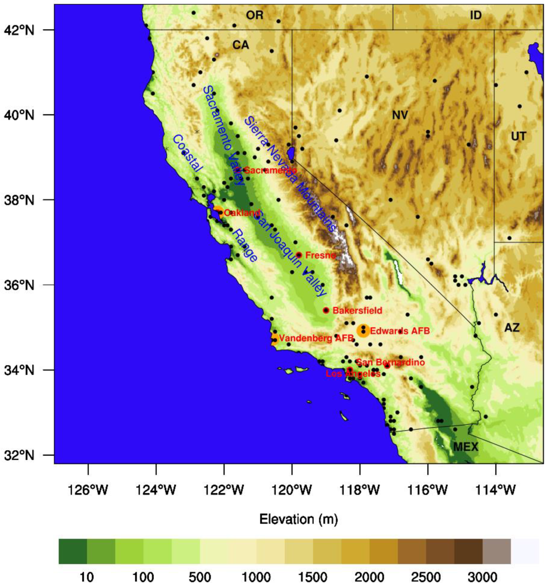
Figure 1. The locations of 161 surface meteorological stations (black dots), 3 rawinsonde stations (orange dots, red labels; Oakland, Vandenberg AFB and Edwards AFB), along with 6 surface stations (black dots, red labels; Oakland, Sacramento, Fresno, Bakersfield, Los Angeles, and San Bernardino that were used to show temporal model evaluations in the manuscript) placed over the terrain relief map over California and neighboring states, Oregon (OR), Idaho (ID), Utah (UT), Arizona (AZ), and country of Mexico (MEX) (black capital letters). Sacramento Valley (SV) and San Joaquin Valley (SJV) are also shown with elevated terrain that surrounds them, namely Coastal Ranges and the Sierra Nevada Mountains (all were highlighted with blue text).
Atmosphere 15 01248 g001
Figure 2. Global MPAS modeling domain setup using varying resolution ranging from 3 to 48 km, where 3 km covers the states of California and Nevada (see Figure S2 for the area of focus, or the evaluation domain used in this study).
Atmosphere 15 01248 g002
Figure 3. Horizontal spatial distribution of (a) 10 m wind vectors, (b) 2 m temperature, and (c) 2 m relative humidity fields that are temporally averaged at 8 AM for the winter 2013 episode from WRF (left), global MPAS (middle) and regional MPAS (right) results.
Atmosphere 15 01248 g003
Figure 4. Temporal evolution of 2 m temperature, 2 m mixing ratio, 2 m relative humidity, and 10 m wind speed and direction predicted by global MPAS (blue), regional MPAS (red), and WRF (green) against the observations (black) at Bakersfield during 10–24 January 2013, episode.
Atmosphere 15 01248 g004
Figure 5. Diurnal evolution of (a) mean bias (BIAS), (b) mean absolute error (MAE), and (c) mean standard deviation (SDEV) of 2 m temperature, and diurnal evolution of (d) mean bias (BIAS), (e) mean absolute error (MAE), and (f) mean standard deviation (SDEV) of 2 m mixing ratio that are averaged over the California evaluation domain for 2013 winter episode.
Atmosphere 15 01248 g005
Figure 6. Rawinsonde observations (upper left) and model predictions of global MPAS (upper right), regional MPAS (lower right) and WRF (lower left) on 15 January 2013, 00Z at Oakland, CA are given in skew-T/log-P diagram. Black line is the observed temperature, blue line is the dew point temperature, and wind barbs on the right show the wind speed and direction with height.
Atmosphere 15 01248 g006
Figure 7. Horizontal spatial distribution of (a) 10 m wind vectors, (b) 2 m temperature, and (c) 2 m relative humidity that are temporally averaged at 8 AM during the summer 2016 episode from WRF (left), global MPAS (middle) and regional MPAS (right) results.
Atmosphere 15 01248 g007aAtmosphere 15 01248 g007b
Figure 8. Temporal evolution of 2 m temperature, 2 m mixing ratio, 2 m relative humidity, 10 m wind speed and direction at Bakersfield, CA during 18–31 July 2016 episode, as estimated by global MPAS (blue), regional MPAS (red) and WRF (green) against observations (black).
Atmosphere 15 01248 g008
Figure 9. Diurnal evolution of bias (BIAS), mean absolute error (MAE) and standard deviation (SDEV) of 2 m temperature (ac) and 2 m mixing ratio (df) that are averaged over the evaluation domain for 2016 summer episode.
Atmosphere 15 01248 g009
Figure 10. Rawinsonde observations (upper left) and model predictions of global MPAS (upper right), regional MPAS (lower right) and WRF (lower left) on 20 July 2016, 12Z at Oakland, CA are given in skew-T/log-P diagram. Black line is the observed temperature, blue line is the dew point temperature, and wind barbs on the right show the wind speed and direction with height.
Atmosphere 15 01248 g010
Disclaimer/Publisher’s Note: The statements, opinions and data contained in all publications are solely those of the individual author(s) and contributor(s) and not of MDPI and/or the editor(s). MDPI and/or the editor(s) disclaim responsibility for any injury to people or property resulting from any ideas, methods, instructions or products referred to in the content.