A Method Based on Deep Learning for Severe Convective Weather Forecast: CNN-BiLSTM-AM (Version 1.0)

Abstract

In this study, we propose a model called CNN-BiLSTM-AM that utilizes deep learning techniques to forecast severe convective weather based on ERA5 hourly data and observations. The model integrates a CNN with a Bidirectional Long Short-Term Memory (BiLSTM) system and an Attention Mechanism (AM). The CNN is tasked with extracting features from the input data, while the BiLSTM effectively captures temporal dependencies. The AM enhances the results by considering the impact of past feature states on severe weather phenomena. Additionally, we assess the performance of our model in comparison to traditional network architectures, including ConvLSTM, Predrnn++, CNN, FC-LSTM, and LSTM. Our results indicate that the CNN-BiLSTM-AM model exhibits superior accuracy in precipitation forecasting. Especially with the extension of the forecast time, the model performs well across multiple evaluation metrics. Furthermore, an interpretability analysis of the convective weather mechanisms utilizing machine learning highlights the critical role of total precipitable water (PWAT) in short-term heavy precipitation forecasts. It also emphasizes the significant impact of regional variables on convective weather patterns and the role of convective available potential energy (CAPE) in fostering conditions conducive to convection. These findings not only confirm the effectiveness of deep learning in the automatic identification of severe weather features but also validate the suitability of the sample dataset employed. Given its remarkable performance and robustness, we advocate for the adoption of this model to enhance the forecast of severe convective weather across various business applications.

1. Introduction

Severe convective weather primarily encompasses violent atmospheric phenomena that occur over limited spatial and temporal scales, including hailstorms, thunderstorms, strong gusts, brief episodes of intense rainfall, tornadoes, and various hazardous weather conditions. The forecasting of severe convective weather, characterized by its localized intensity and rapid development, poses considerable challenges [1,2]. This type of weather often manifests in extreme conditions that can result in significant loss of life and extensive property damage [3]. Notable instances include the sinking of the “Eastern Star” vessel in 2015 [4], the EF4 tornado that struck Funing, Jiangsu Province, in 2016 [5], and the extensive “720” torrential rain event that occurred in Zhengzhou, Henan, in 2021 [6].

Numerous researchers employ models for numerical weather prediction (NWP), including the Weather Research and Forecasting (WRF) model and the Global Forecast System (GFS), which are considered essential tools for forecasting severe convective weather events [7,8]. These models are particularly critical for providing early warnings [9]. However, a significant challenge arises from the inherent instability of the atmosphere, which complicates the ability of current numerical atmospheric models to accurately forecast the timing, location, and intensity of severe convective weather phenomena. Kryza et al. [10] conducted a study utilizing the WRF model to forecast short-duration intense rainfall in southwestern Poland. Their results demonstrated that all configurations of the model tested were unable to accurately replicate local intense precipitation events. To address this limitation, Hamill et al. [11] implemented an ensemble forecasting approach aimed at enhancing the precipitation forecast capabilities of the WRF model. While ensemble forecasting can partially reflect the forecasting ability or reliability of the actual atmosphere, it does not improve the underlying physical mechanisms within the models. The GFS model is distinguished as a globally recognized weather forecasting system, providing weather forecasts on a worldwide scale. It processes a comprehensive array of observational data from various sources, including satellites, meteorological stations, radars, and buoys, to establish its initial conditions. However, since the 1980s, the hydrostatic spectral dynamical core of the GFS has not undergone significant upgrades, despite advancements in spatial resolution, energy conservation, and computational efficiency [12,13,14,15,16]. Although a global nonhydrostatic spectral model could theoretically be developed [17], its scalability issues render it impractical for future computational frameworks. Consequently, adapting the GFS spectral dynamical core to nonhydrostatic scales for the forecast of convective-scale events, which require grid spacing smaller than 4 km, is largely considered unfeasible [18,19,20,21]. NWP is pivotal in forecasting severe convective weather by modeling atmospheric phenomena through mathematical and physical equations. Nevertheless, the numerical prediction process is fraught with uncertainties, such as inaccurate initial conditions and the parameterization of physical phenomena. The chaotic nature of the atmosphere exacerbates these inaccuracies, leading to significant doubts regarding the outcomes produced by the models [22]. Despite the uncertainties and challenges inherent in the model system, advancements in observational technologies, data assimilation techniques, model resolutions, physical parameterizations, and statistical post-processing of model outputs over the past two decades have markedly improved the forecast accuracy of numerical weather models. Nonetheless, the model system continues to face numerous challenges and uncertainties that necessitate further investigation and resolution.

In recent years, significant advancements in artificial intelligence (AI) have catalyzed transformations across various domains. AI, particularly through its foundations in deep learning (DL) and machine learning (ML), has achieved remarkable progress, providing robust solutions in multiple areas. When these technologies are combined with extensive meteorological data, they form a powerful toolkit for forecasting severe weather [23,24]. Through the application of the random forest algorithm, Li et al. [25] successfully identified and forecasted severe weather phenomena, including intense short-term rainfall, thunderstorms, hail, and other extreme conditions. Their methodology incorporated convective indices and measurable physical properties, as well as real-time forecasting data, into the model. An analysis of 85 cases of severe weather revealed a mere 21.9% error rate, with no instances overlooked, thereby demonstrating the high reliability of their model for forecasting severe weather events. In a separate study, Herman and Schumacher [26] developed a machine learning (ML) model that integrates various predictors, such as temperature, humidity, pressure, and wind dynamics, alongside statistical background elements, including extremes and medians of specific climatic variables over designated recurrence intervals. They illustrated the model’s efficacy in accurately forecasting extreme precipitation up to three days in advance. Liu et al. [27] employed Bayesian analysis to explore the relationship between thermal and dynamic factors within storm clouds that produce frequent lightning. They underscored the importance of variables such as convective available potential energy, inhibition energy, and low-level wind shear in predicting these high-frequency lightning events. In contrast to simpler ML approaches, deep learning (DL) excels in managing complex nonlinear interactions and achieves higher levels of abstraction, thereby outperforming traditional models in various applications, including speech and image processing [28,29,30]. Moreover, DL is increasingly being applied to short-term weather forecasts. Lin et al. [31] developed a framework known as ConvLSTM, based on the Weather Research and Forecasting (WRF) model, with the objective of predicting lightning occurrences over the subsequent 12 h with improved spatiotemporal accuracy. Additionally, Gope et al. [32] designed a model for forecasting severe rainstorms utilizing deep neural networks, specifically stacked autoencoders, which leveraged historical weather data. This model demonstrated the capability to forecast heavy rainfall in cities such as Mumbai and Kolkata, India, well in advance, with lead times ranging from 6 to 48 h.

As small and medium-scale observational networks continue to advance, the diversity of observational techniques expands, and the volume of observational data increases rapidly, it is imperative to investigate the origins and evolution mechanisms of each severe convective weather event. Distinguishing the unique parameters and threshold values for various types of severe convective weather within extensive datasets derived from numerical models is essential. Furthermore, considering the specific geographic and climatic conditions of each region is critical for the accurate forecast of severe convective weather events. Deep learning (DL) algorithms are proficient in identifying key characteristics within large datasets, efficiently extracting valuable information while accounting for geographic and climatic variations across different areas. The innovative “Pangu-Weather” model demonstrates exceptional performance in forecasting wind velocity and temperature, exhibiting notable precision and rapid computation times [33]. Another innovative model “GraphCast” utilizes machine learning techniques trained on reanalysis data to provide forecasts for various atmospheric variables globally at a resolution of 0.25° over a 10-day period, generating these forecasts in under one minute. In terms of forecasting accuracy, GraphCast outperforms the most reliable operational deterministic models in 90% of the 1380 verification cases, thereby significantly enhancing the forecast of severe convective weather phenomena [34].

This research employs ERA5 hourly data alongside observational data to apply deep learning (DL) algorithms in the creation of a forecasting model for severe convective weather, referred to as CNN-BiLSTM-AM. The model is designed to produce hourly precipitation forecasts for the subsequent 0–6 h, with the potential to enhance forecast accuracy by effectively capturing high-impact factors and features associated with severe convective weather phenomena. Furthermore, it offers an opportunity for improved efficiency by utilizing contemporary DL hardware, thereby reducing reliance on supercomputers and achieving more favorable speed–accuracy trade-offs. In addition to its applications in meteorological forecasting, this research lays the groundwork for addressing other significant geo-spatiotemporal forecasting challenges, including those related to climate and ecology, energy, agriculture, human and biological activities, and complex dynamical systems.

2. Data and Methods

2.1. ERA5

To train and evaluate the CNN-BiLSTM-AM model, we utilized a subset of the European Centre for Medium-Range Weather Forecasts (ECMWF) ERA5 archive. ERA5 represents the fifth generation of reanalysis data produced by ECMWF, utilizing the Integrated Forecasting System (IFS cycle 41r2) as its foundation. This dataset offers extensive information regarding global atmospheric changes since 1940. In contrast to its predecessor, ERA-Interim, ERA5 incorporates advancements in both the atmospheric model and the assimilation system, while also integrating a greater volume of observational data [35]. As the most recent reanalysis product from ECMWF, ERA5 features a spatial resolution of 0.25 degrees and a temporal resolution of 1 h.

To improve the forecast accuracy of the model and accelerate the training process, we initially select and calculate a range of predictors from the extensive variables available in ERA5. These predictors represent critical environmental conditions that are conducive to severe convective weather events. They include various convective physical parameters that effectively capture water vapor content, atmospheric instability, and uplift conditions. Notably, the physical parameters considered include convective available potential energy (CAPE), precipitable water (PWAT), convective inhibition (CIN), and wind shear. To account for geographical variations across different regions, we also incorporate longitude and latitude into our model. We employed a variety of meteorological variables to compute the indices for each grid cell, including pressure, temperature, relative humidity, geopotential height, vertical velocity, and wind vector. Utilizing these parameters, we derived the thermodynamic, kinematic, composite, and humidity indices for each grid cell. In total, we identified 20 parameters (see

Table 1. Selected predictors for severe convective weather forecasting in the study.

Group	Abbreviation	Parameter Name
Thermodynamic instability parameters	LI CAPE CIN LR DACPE DCI SP WBZ	Lifted index Convective available potential energy Convective inhibition Temperature lapse rate at different levels Downdraft convective available energy Deep convective index Surface pressure Wet bulb zero
Kinematic parameters	Shear3 km Shear1 km WMAX Wmid	Bulk wind shear Bulk wind shear Maximum potential speed of an updraft Mean of the vertical velocities
Humidity parameters	Td850 PWAT MRH HI	Dew point temperature at 850 hPa Precipitable water Mean relative humidity Humidity index
Thermodynamic parameters	T	2 m temperature
Composites	EHI	Energy–Helicity index
Other	LON	Longitude
	LAT	Latitude

) based on our expertise in forecasting convective weather and the successful predictive capabilities demonstrated in other study regions [36,37,38,39,40,41,42,43].

2.2. Observational Data

In this study, the data utilized for labeling predictors were obtained from surface meteorological stations across China and were curated by the National Meteorological Information Center. This center is committed to conducting quality assessments and rectifying errors in both time-specific observations and records of daily extreme values for a comprehensive set of 19 critical meteorological elements. These elements include temperature, pressure, precipitation, humidity, and sunlight duration, collected from over 2400 terrestrial stations throughout the country. Such a systematic approach is essential for identifying and addressing systematic discrepancies that may arise during the data digitization process, including instances of missing or duplicated data. In accordance with the standard procedures of meteorological departments, the data undergoes a three-tiered quality assurance evaluation at the station, provincial, and national levels.

2.3. Deep Learning Method

2.3.1. Training/Testing Sets

The ERA5 hourly data are characterized by grid-based fields, in contrast to the scattered nature of observed data, necessitating a gridding process for the latter. When a weather event associated with a specific timeframe occurs within a grid radius denoted as R, it indicates the presence of the event at that particular grid location. Conversely, if the weather event is situated outside the defined grid radius, it signifies the absence of the event at that grid position. Given the typical association of convective weather with mesoscale systems, our research adopted an R value of 20 km. A very small R may result in the oversight of critical severe convective weather incidents, while an excessively large R could lead to the issuance of unwarranted alerts. The probability of encountering severe convective weather conditions is notably low, resulting in a significant imbalance where instances of severe convective occurrences are substantially outnumbered by those lacking such events. This situation exemplifies the challenges posed by imbalanced data [44]. To address this issue, we implemented an oversampling strategy, which involved the random replication of positive instances to achieve a more balanced distribution between positive and negative instances [45]. Distinct datasets were created utilizing ERA5 hourly data and observational records from 2015 to 2020. The initial five years (2015–2019) were designated as the training set, while the final year (2020) was reserved for testing purposes.

2.3.2. CNN-BiLSTM-AM Model

In order to enhance the accuracy of forecasting severe convective weather events, we propose a model designated as CNN-BiLSTM-AM (see Figure 1). This model integrates a Convolutional Neural Network (CNN), a Bidirectional Long Short-Term Memory (BiLSTM) system, and an Attention Mechanism (AM). The CNN component is tasked with extracting features from the incoming dataset, while the BiLSTM module is specifically designed to effectively recognize temporal correlations within sequential data. Furthermore, the AM aims to improve forecast performance by considering how previous states of features influence instances of intense precipitation [46]. The analysis of historical meteorological imagery and numerical data is crucial in the weather forecasting process. To succinctly encapsulate this methodology, the initial step involves examining various forecasting products to establish situational forecasts. This is subsequently followed by the integration of these forecasts with current local meteorological statistics to achieve precise forecasting elements. In simpler terms, the initial phase consists of deriving features from meteorological images or forecasted outputs, while the subsequent phase aligns these extracted features with historical local meteorological data to deduce the desired forecasting figures. Within the framework of CNN-BiLSTM-AM, these stages are adapted by utilizing the CNN for data feature extraction, which is then integrated with historical meteorological data through the application of BiLSTM and AM to finalize the forecasted elements. Prior to inputting the data into the CNN-BiLSTM-AM framework, it is essential to standardize the data and reshape it into a matrix format. Following these preparatory steps, the framework is prepared for training.

The training process for the CNN-BiLSTM-AM model involves the following steps: (1) Provision of input data. (2) Application of Equation (1) [46] to standardize the input data, thereby reducing significant discrepancies. (3) Initialization of weights and biases across various layers. (4) Feature extraction and generation of output values. (5) Execution of computations within the BiLSTM layer. (6) Processing in the AM layer: The AM layer is employed to further refine the output obtained from the BiLSTM layer. (7) Evaluation of termination conditions: assessment of whether the termination criteria have been satisfied, which may include the completion of training cycles or the attainment of specified thresholds for weight adjustments or prediction errors.

$$y_i={\displaystyle \frac{x_i-\overline{x}}{s}}$$

(1)

Here, ${\mathrm{y}}_{\mathrm{i}}$ represents the standardized value, ${\mathrm{x}}_{\mathrm{i}}$ stands for the input data, $\overline{\mathrm{x}}$ denotes the mean of the input data, and s signifies the standard deviation of the input data.

The sequence of actions for making predictions using the CNN-BiLSTM-AM model is delineated as follows: (1) Provision of input data: this step involves supplying the necessary data for forecasting. (2) Data standardization: this entails standardizing the provided input data to ensure consistency. (3) Prediction generation: the normalized data are then input into the previously trained CNN-BiLSTM-AM model to obtain the output values. (4) Reversion of data standardization: Equation (2) [46] is employed to revert the outputs to their original form. (5) Presentation of final outputs: the results, following the reversion process, are displayed as the concluding step in the prediction sequence.

$${\mathrm{x}}_{\mathrm{i}}={\mathrm{y}}_{\mathrm{i}}·\mathrm{s}+\overline{\mathrm{x}}$$

(2)

Here, ${\mathrm{x}}_{\mathrm{i}}$ stands for the retrieved value of the standardized figure, ${\mathrm{y}}_{\mathrm{i}}$ indicates the CNN-BiLSTM-AM output, s symbolizes the deviation standard of input data, and $\overline{\mathrm{x}}$ denotes the average input data value.

During the training phase, the ADAM optimizer was utilized [47], with a learning rate set at 10⁻⁴, while default configurations were maintained for all other parameters [48]. The model training process incorporated an early stopping strategy, with the number of epochs established at 300. If the loss did not exhibit a decrease for more than 10 consecutive epochs, the training process was automatically terminated. A batch size of 16 was employed. The loss function chosen for minimization during training was the mean squared error (MSE), which is defined by the following formula [48]:

$$MSE={\displaystyle \frac{1}{m}}\sum _{i=1}^m{(y_i^{\prime }-y_i)}^2$$

(3)

where m represents the training sample size, ${\mathrm{y}}_{\mathrm{i}}$ represents the actual value, and ${\mathrm{y}}_{\mathrm{i}}^{\prime }$ represents the predicted value.

2.4. Experimental Area

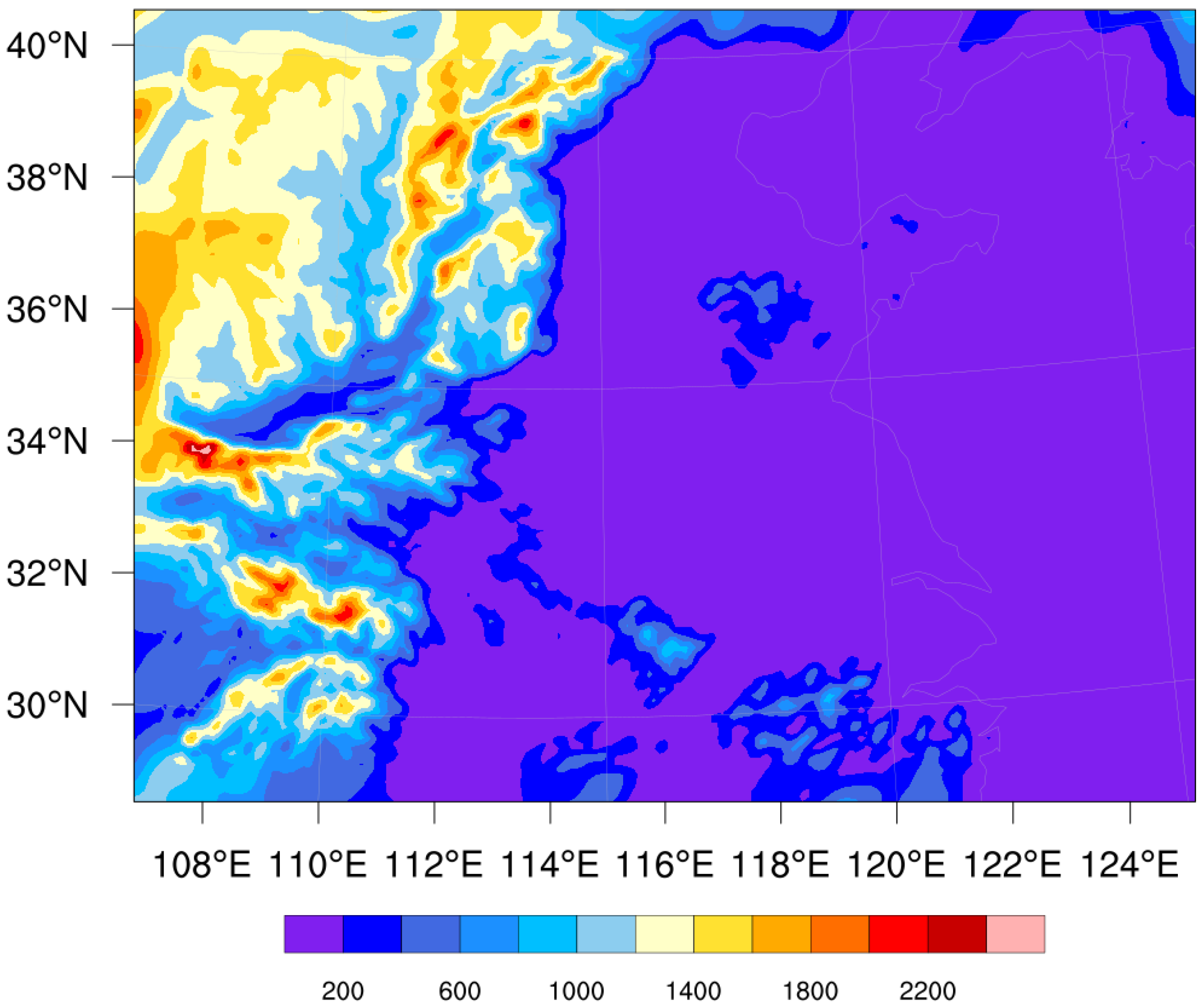
The Henan region serves as a vital center for agricultural production in China and exemplifies the convergence of urban and rural landscapes within a complex topographical framework, largely influenced by extensive industrial activities. Additionally, its mid-latitude location renders the area susceptible to incursions of cold air, while it simultaneously attracts warm, moist air currents during the summer months. This interaction frequently results in significant precipitation due to the confluence of these distinct air masses. Furthermore, there is an increasing body of evidence indicating a transition in China’s climate, which may lead to heightened summer rainfall, particularly in northern regions. Consequently, selecting Henan (illustrated in Figure 2) as the primary focus of this investigation is well-aligned with the study’s objectives. This decision is not only forward-looking but also strategically astute.

2.5. Evaluation Methods

Verification metrics commonly employed to assess the accuracy of forecasts encompass the Threat Score (TS), Probability of Detection (POD), False Alarm Rate (FAR), Equitable Threat Score (ETS), Ratio of Missed Alarms (MAR), and Bias Factor (BIAS) [49,50,51,52,53]. The definitions of these metrics are as follows:

$$TS={\displaystyle \frac{h}{h+m+f}}$$

(4)

$$POD={\displaystyle \frac{h}{h+m}}$$

(5)

$$FAR={\displaystyle \frac{f}{h+f}}$$

(6)

$$ETS={\displaystyle \frac{h-h_{random}}{h+f+m+-h_{random}}},h_{random}={\displaystyle \frac{(h+f)\ast (h+m)}{(h+m+f+c)}}$$

(7)

$$MAR={\displaystyle \frac{m}{h+m}}$$

(8)

$$BIAS={\displaystyle \frac{h+f}{h+m}}$$

(9)

Here, h denotes the frequency of instances where both the forecasted events and observed events are present. The variable m, on the other hand, signifies the frequency of occurrences where the observed event is present but not the forecasted event. Additionally, f stands for the frequency of cases where the forecasted event is present while the observed event is absent. Lastly, c indicates the frequency of events where neither the forecasted nor observed events are present.

When evaluating the model’s performance, various assessment metrics are frequently used, such as the correlation coefficient (r), root mean square error (RMSE), and standard deviation (${\mathsf{\sigma }}_{\mathrm{n}}$) [49,50,51,52,53]. Below are the specific formulas for these metrics:

$$r={\displaystyle \frac{\sum _{i=1}^N\left(S_i-\overline{S}\right)(O_i-\overline{O})}{\sqrt{\sum _{i=1}^N{(S_i-\overline{S})}^2}\sqrt{\sum _{i=1}^N{(O_i-\overline{O})}^2}}}$$

(10)

$$RMSE=\sqrt{{\displaystyle \frac{\sum _{i=1}^N{\left(S_i-O_i\right)}^2}{N}}}$$

(11)

$${\sigma }_n={\displaystyle \frac{\sqrt{\sum _{i=1}^N{(S_i-O_i)}^2}}{N}}$$

(12)

where S denotes the value predicted, O denotes the ground observation, $\overline{\mathrm{O}}$ denotes the average ground observation, $\overline{\mathrm{S}}$ denotes the average predicted value, i represents the number of samples, and N represents the total number of samples used in the study.

3. Results

3.1. Evaluation of Different DL Models

To assess the performance of the CNN-BiLSTM-AM model, we conduct a comparative analysis with several algorithms, including ConvLSTM [49], Predrnn++ [50], CNN [51], FC-LSTM [52], and LSTM [53]. ConvLSTM represents a variant of the Long Short-Term Memory (LSTM) model that integrates convolutional operations alongside recurrent connections. This model was developed to address sequential data processing tasks characterized by spatial dependencies, such as those found in video and image sequences. In the ConvLSTM framework, the input sequence is conceptualized as a two-dimensional grid, with each element corresponding to a frame or an image [49]. Predrnn++ enhances the architecture of Predrnn by incorporating ConvLSTM cells in conjunction with a spatial–temporal attention mechanism, which facilitates the capture of long-term dependencies and the generation of precise predictions. The spatial–temporal attention mechanism employed in Predrnn++ allows the model to selectively focus on informative regions and time steps within the video sequence, thereby improving prediction accuracy [50]. CNN, or Convolutional Neural Network, is a deep learning algorithm widely applied in computer vision tasks, including image classification, object detection, and image recognition. During the training phase, CNNs are optimized through backpropagation and gradient descent algorithms. By adjusting the weights of the convolutional filters and the parameters of the fully connected layers, the network learns to identify specific patterns and objects within the input images [51]. The FC-LSTM architecture merges the advantages of both LSTM and fully connected layers, utilizing the robust memory and sequential modeling capabilities of LSTM units alongside the capacity of fully connected layers to capture intricate relationships within the data [52]. LSTM, a specific type of recurrent neural network (RNN) architecture, is designed to mitigate the vanishing gradient problem that may arise when training deep neural networks on sequential data. Sequential data, such as time series, text, or speech, frequently exhibits long-term dependencies, wherein information from earlier time steps is pertinent for making accurate predictions at subsequent time steps [53].

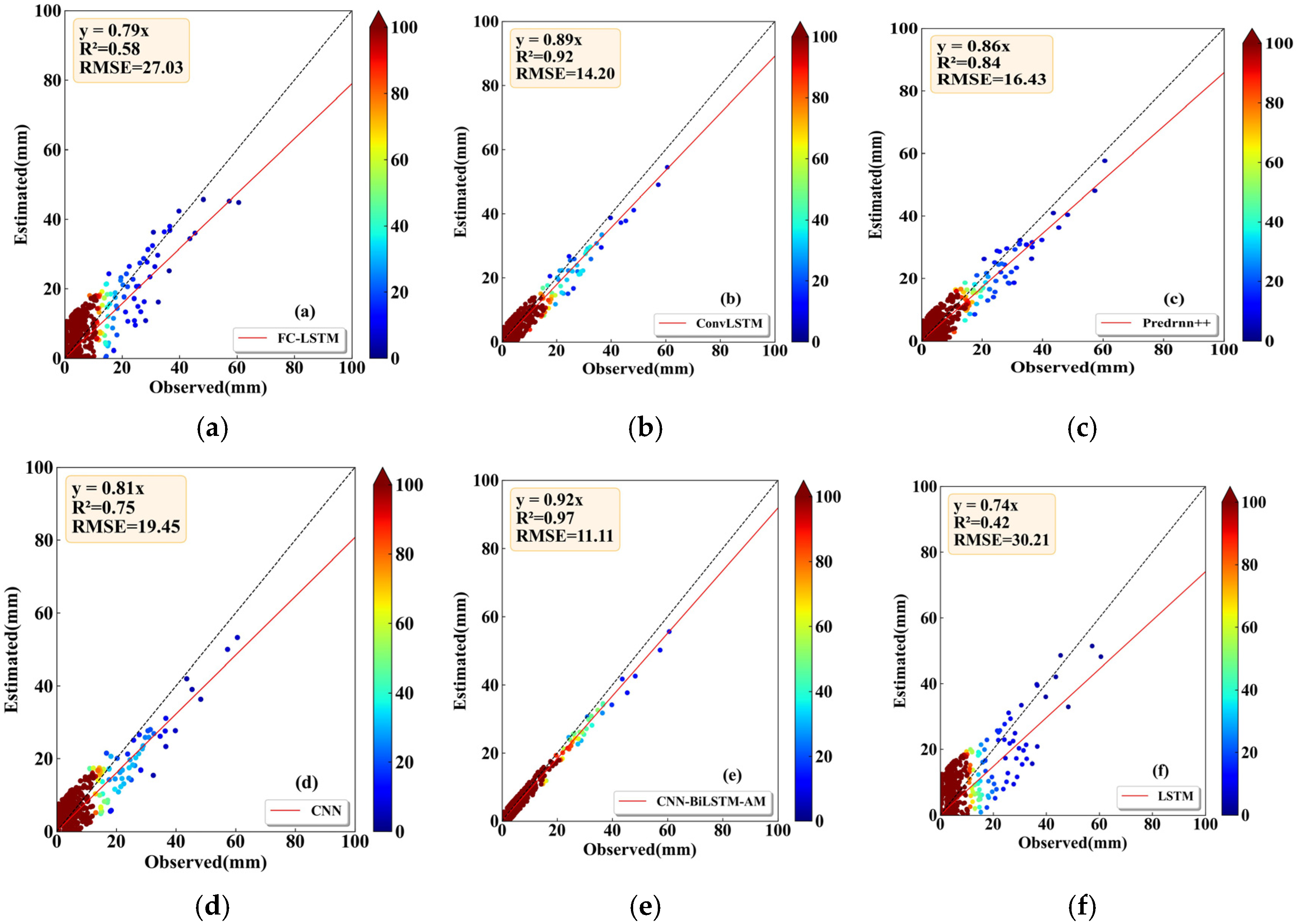
In this study, we utilize a training dataset to train the model and a testing dataset to forecast hourly precipitation. To ensure a fair comparison, all models are trained on the same dataset, and all parameters are optimized according to the specific context. Figure 3 illustrates the scatter density plot of the errors between the predicted and actual precipitation values generated by the six models under consideration. From Figure 3, it is evident that the Long Short-Term Memory (LSTM) model exhibits the poorest performance, with a root mean square error (RMSE) value of 30.21 mm. In contrast, the Convolutional Neural Network (CNN) and Fully Convolutional LSTM (FC-LSTM) models demonstrate superior performance, as indicated by their RMSE values of 19.45 mm and 27.03 mm, respectively. These figures represent error reductions of 35.62% and 10.53% when compared to the LSTM model. Conversely, the ConvLSTM and Predrnn++ models display enhanced forecasting capabilities, as evidenced by their lower RMSE values of 14.20 mm and 16.43 mm, respectively, translating to error reductions of 53.00% and 45.61% relative to the LSTM approach. Furthermore, these models exhibit stronger correlation coefficients, indicating a higher degree of correlation between predicted and actual precipitation. Despite the favorable results obtained from the ConvLSTM and Predrnn++ models, the CNN-BiLSTM-AM model presented in this study outperforms all others. This model demonstrates a more accurate convergence between forecasted and actual rainfall amounts, resulting in the least overall discrepancy. Specifically, the CNN-BiLSTM-AM model achieves an RMSE of only 11.11 mm, reflecting significant error reductions of 63.22%, 42.88%, 58.90%, 32.38%, and 21.76% compared to the LSTM, CNN, FC-LSTM, Predrnn++, and ConvLSTM models, respectively. Additionally, it attains an exemplary correlation coefficient of nearly 97%, indicating a strong correlation between predicted and observed precipitation. In summary, the analysis clearly demonstrates that the CNN-BiLSTM-AM model significantly outperforms traditional deep learning models such as LSTM, CNN, FC-LSTM, Predrnn++, and ConvLSTM in the prediction of rainfall.

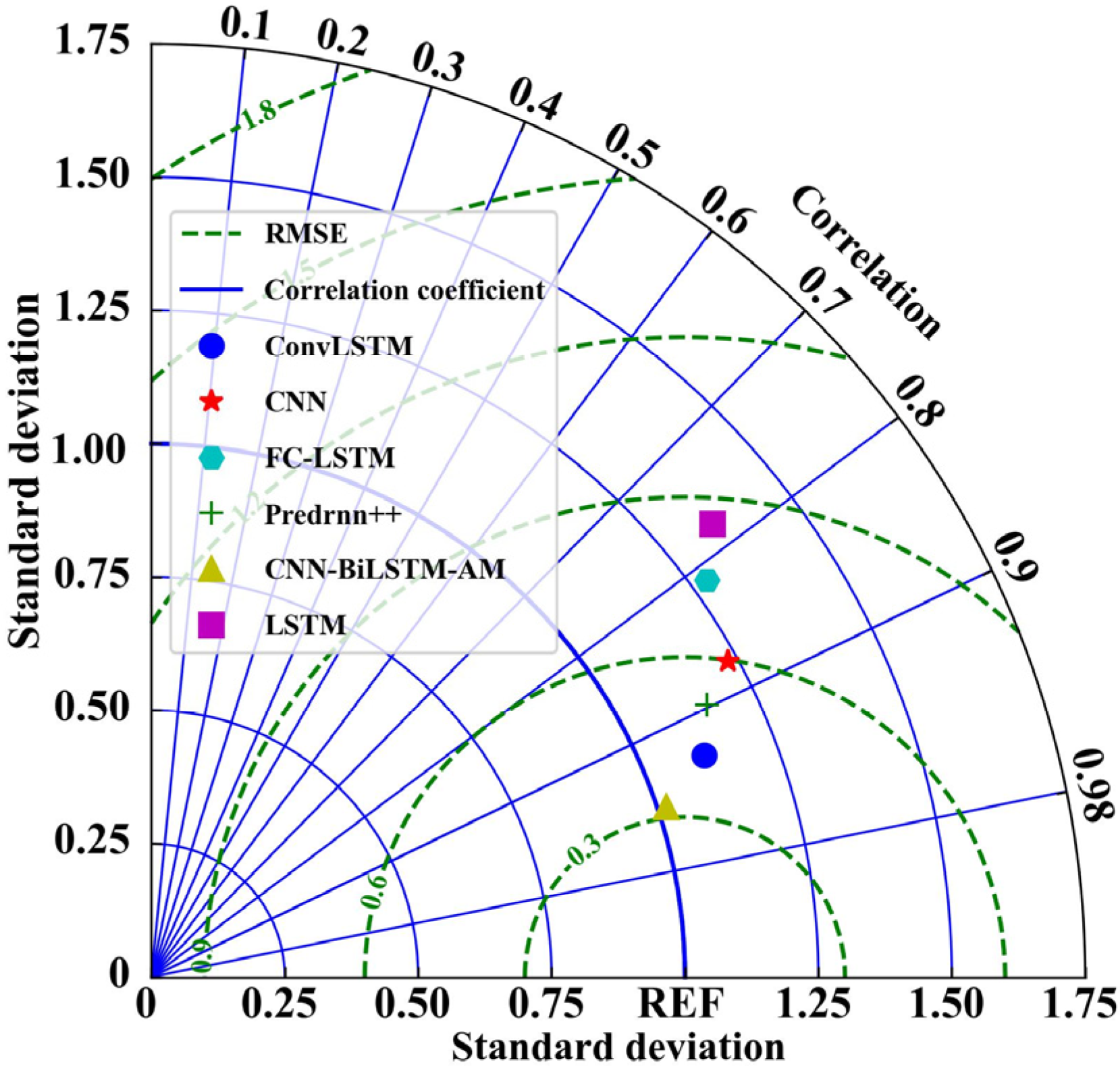
In order to further investigate the reliability of the CNN-BiLSTM-AM model, a comparative analysis was conducted involving five additional models. This analysis utilized cumulative distribution probability scatter plots and Taylor plots (refer to Figure 4). The results indicate that the standard deviation (${\mathsf{\sigma }}_{\mathrm{n}}$) of the CNN-BiLSTM-AM model is 1.02, with a correlation coefficient (r) of 0.97. The ConvLSTM model closely follows as the second most accurate model, exhibiting a standard deviation of 1.12 and a correlation coefficient of 0.92. Conversely, the LSTM model demonstrated the weakest performance, with a standard deviation of 1.30 and a correlation coefficient of 0.78. The accuracy metrics for the FC-LSTM, CNN, and Predrnn++ models are situated between these extremes. In conclusion, the proposed CNN-BiLSTM-AM model exhibits superior performance in effectively extracting the developmental characteristics of convective weather, thereby enhancing precipitation forecasting capabilities.

3.2. Case Evaluation

On 22 July 2022, the regions of Henan and central Inner Mongolia in China experienced significant thunderstorms accompanied by short-term heavy precipitation. The efficacy of rainfall prediction is illustrated in

Table 2. Comparative analysis of different models for convective weather event on 22 July 2022.

	Forecast Duration	POD	FAR	$\mathbf{E}\mathbf{T}\mathbf{S}$	TS
CNN-BiLSTM-AM	1 h	0.586	0.395	0.462	0.493
	2 h	0.498	0.444	0.433	0.452
	3 h	0.445	0.461	0.372	0.381
	4 h	0.423	0.491	0.323	0.344
	5 h	0.411	0.542	0.301	0.313
	6 h	0.382	0.613	0.222	0.231
Predrnn++	1 h	0.544	0.412	0.451	0.459
	2 h	0.402	0.465	0.313	0.326
	3 h	0.364	0.481	0.242	0.273
	4 h	0.315	0.521	0.190	0.203
	5 h	0.302	0.591	0.161	0.185
	6 h	0.283	0.635	0.122	0.165
ConvLSTM	1 h	0.554	0.411	0.453	0.459
	2 h	0.430	0.452	0.335	0.389
	3 h	0.379	0.481	0.303	0.327
	4 h	0.358	0.510	0.263	0.281
	5 h	0.322	0.583	0.195	0.242
	6 h	0.293	0.622	0.133	0.176
CNN	1 h	0.534	0.422	0.431	0.443
	2 h	0.394	0.481	0.263	0.282
	3 h	0.357	0.503	0.220	0.237
	4 h	0.309	0.531	0.185	0.191
	5 h	0.276	0.593	0.172	0.181
	6 h	0.223	0.642	0.125	0.133
FC-LSTM	1 h	0.480	0.436	0.425	0.432
	2 h	0.373	0.496	0.245	0.259
	3 h	0.332	0.513	0.216	0.224
	4 h	0.303	0.536	0.175	0.184
	5 h	0.240	0.612	0.142	0.150
	6 h	0.215	0.653	0.116	0.131
LSTM	1 h	0.433	0.452	0.421	0.423
	2 h	0.356	0.503	0.225	0.237
	3 h	0.313	0.524	0.204	0.219
	4 h	0.297	0.595	0.170	0.188
	5 h	0.224	0.620	0.125	0.142
	6 h	0.206	0.675	0.116	0.129

. Insights derived from this table indicate varying levels of forecast accuracy across different algorithms. Among the six algorithms evaluated, the CNN-BiLSTM-AM model demonstrates superior forecasting capabilities. During the 1–6 h forecast period, its Probability of Detection (POD) and Threat Score (TS) values are as follows: 0.586, 0.498, 0.442, 0.423, 0.401, 0.382, 0.493, 0.452, 0.381, 0.344, 0.313, and 0.231, respectively. In comparison, the ConvLSTM model, which ranks second, shows improvements of 5.78%, 15.81%, 17.41%, 18.16%, 27.64%, and 30.38% for POD and 7.41%, 16.20%, 16.51%, 22.42%, 29.34%, and 31.25% for TS, respectively. As the prediction interval increases, the CNN-BiLSTM-AM consistently outperforms its counterparts. Notably, at the 3 h forecast mark, the differences in TS values between CNN-BiLSTM-AM and other models, such as Predrnn++, ConvLSTM, CNN, FC-LSTM, and LSTM, are 0.108, 0.054, 0.144, 0.157, and 0.162, reflecting enhancements of 39.56%, 16.51%, 60.76%, 70.09%, and 73.97%, respectively. By the 6 h forecast, these differences are recorded as 0.064, 0.055, 0.098, 0.100, and 0.102, indicating advancements of 40.00%, 31.25%, 73.68%, 76.34%, and 79.07%, respectively. It is worth noting that the CNN-BiLSTM-AM model has a higher POD and a lower FAR compared to other models, making it a more conservative forecast. At the same time, this model performs better in terms of ETS, TS, and other metrics, providing better guidance and effectively assisting forecasters. This analysis underscores the exceptional performance of the CNN-BiLSTM-AM model in the context of rainfall forecasting.

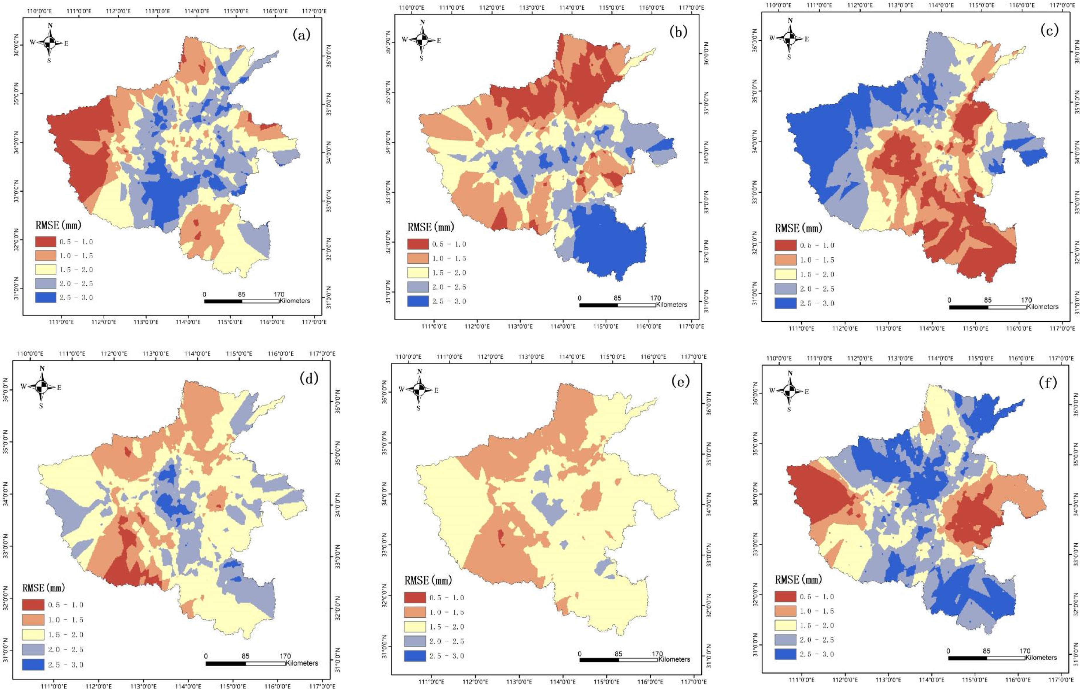
To facilitate a more intuitive comparison, we visualized the distribution of root mean square error (RMSE) values from various models, as illustrated in Figure 5. The RMSE values associated with the CNN-BiLSTM-AM model predominantly range from 0.5 mm to 2.0 mm. In contrast, the performance of the FC-LSTM, ConvLSTM, Predrnn++, CNN, and LSTM models is comparatively inferior to that of the CNN-BiLSTM-AM. The RMSE values for these models are as follows: FC-LSTM: 1.0 mm to 3.0 mm; ConvLSTM: 0.5 mm to 2.5 mm; Predrnn++: 0.5 mm to 2.5 mm; CNN: 0.5 mm to 2.5 mm; and LSTM: 1.0 mm to 3.0 mm. These results indicate that the CNN-BiLSTM-AM model significantly enhances the accuracy of precipitation predictions during intense rainfall events, thereby providing forecasters with valuable insights and benchmarks.

To further validate the performance of the CNN-BiLSTM-AM model, Skamarock et al. [54] applied WRF4.0 to forecast this weather event, using ERA5 reanalysis data as the model’s initial field and boundary conditions. The horizontal resolution is set at 0.25° × 0.25°, employing triple nesting, with the center of the simulation area located at (34.47° N, 114.21° E). The grid points are set at 151 × 151, 202 × 151, and 220 × 151, corresponding to resolutions of 9 km, 3 km, and 1 km, respectively, with integration time steps set at 54 s, 18 s, and 6 s. The model has a total of 50 vertical layers, with the top pressure at 50 hPa. According to the studies by Gao et al., (2022) [6], the physical processes and schemes selected for the model are mainly shown in

Table 3. Physical process and scheme selection.

Physical Process	Scheme Selection
Cloud microphysical process scheme	Thompson
Near-ground level scheme	Monin-Obukhov
Land surface process scheme	Noah
Boundary layer scheme	YSU
Shortwave radiation scheme	Dudhia
Long-wave radiation scheme	RRTM
Cumulus convection scheme	Kain Fritsch
Cloud microphysical process scheme	Thompson

. The total integration time is 24 h, with the initial integration time set from 00:00 on 22 July 2022 to 00:00 on 23 July, outputting results every hour. We compared the forecast results of the CNN-BiLSTM-AM model with those of the WRF model, and the results showed that from 08:00 to 14:00 on 22 July the forecast scores of the CNN-BiLSTM-AM model consistently outperformed those of the WRF model (see Figure 6). It can be seen that the CNN-BiLSTM-AM model based on deep learning technology performed outstandingly in the forecast of this weather event, providing important references and basis for forecasters.

4. Discussion

4.1. Stability Analysis of the Proposed Models

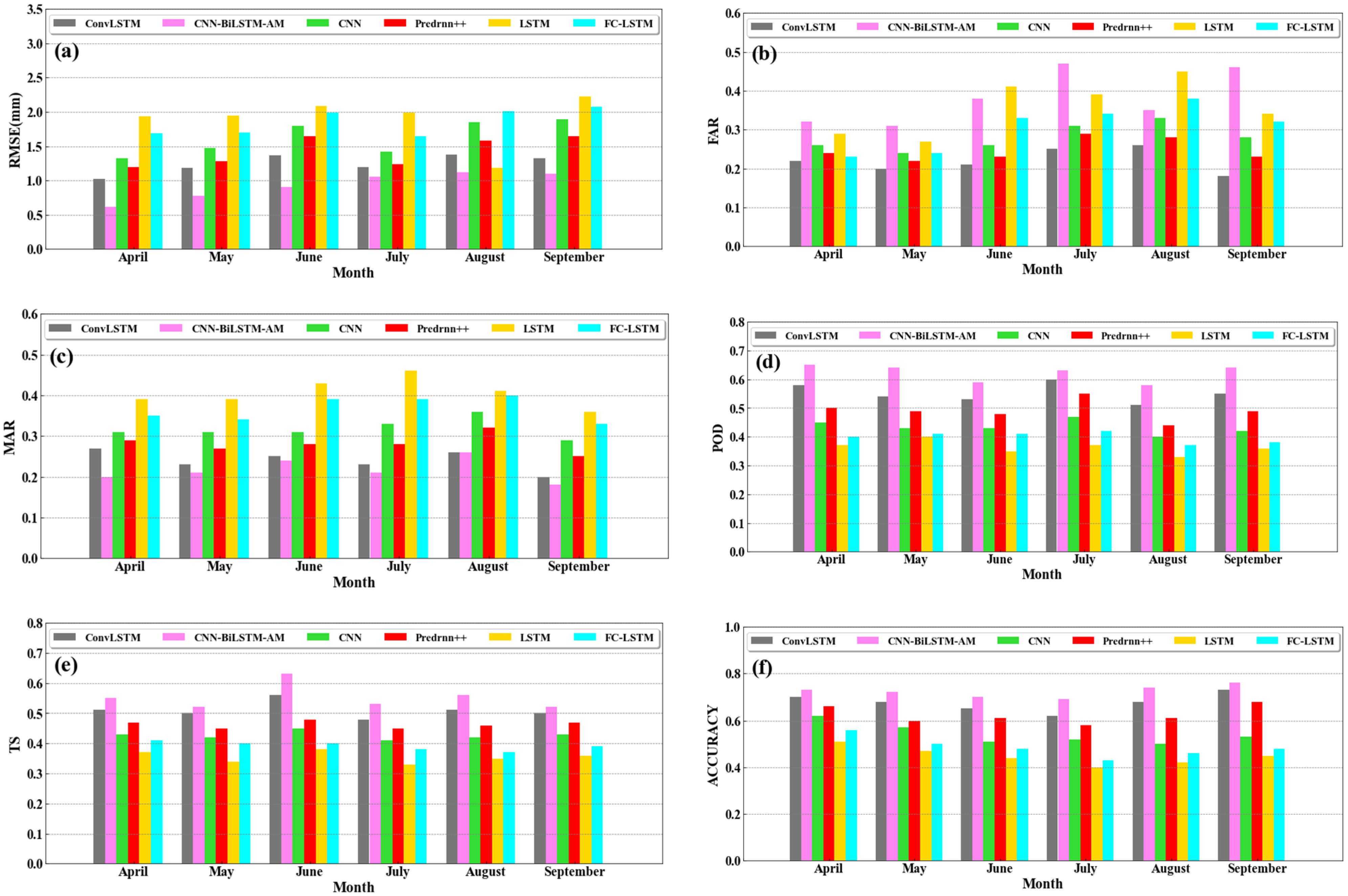
The previous findings presented the visualized results of various deep learning (DL) models, which may not fully capture the consistency across these models. To conduct a more comprehensive evaluation of the stability exhibited by these models, we assess their efficacy in forecasting severe convective weather during the flood season (April–September) from 2020 to 2022. The detailed outcomes of this analysis are illustrated in Figure 7. This thorough examination provides precise insights into the consistency levels of the different models. From Figure 7a, it is evident that the CNN-BiLSTM-AM model demonstrates the lowest RMSE compared to alternative DL algorithms, indicating a significant improvement in precipitation accuracy during the flood season and showcasing its effectiveness in addressing nonlinear issues. The FAR and MAR are critical metrics for evaluating the precision of precipitation forecast, highlighting the rates of false and missed alerts, respectively. Figure 7b,c illustrate that the FAR of the CNN-BiLSTM-AM model outperforms all other models, while its MAR is lower than that of the remaining models. This scenario may be attributed to the CNN-BiLSTM-AM model’s effective capture of precipitation patterns, although it may also lead to unintended consequences, such as forecasting precipitation in the absence of actual events. Notably, the CNN-BiLSTM-AM model exhibits superior performance in POD (Figure 7d), TS (Figure 7e), and overall accuracy (Figure 7f) compared to other DL approaches. These findings suggest that the CNN-BiLSTM-AM model delivers exceptional results in precipitation forecast, surpassing alternative deep learning methodologies.

4.2. The Interpretability Analysis

While machine learning-based techniques have made significant advancements across various domains, the accurate prediction of rainfall through these methods continues to present a “black box” challenge [55], with intricate details often remaining elusive [55]. Currently, numerous researchers are focused on elucidating these “black box” techniques for model interpretation and visualization (MIV). These approaches facilitate a deeper understanding for machine learning users regarding the advantages, limitations, and most appropriate applications of machine learning models. Such comprehension enhances confidence in the models and increases their practical utility. If machine learning predictions exceed those made by human forecasters, MIV techniques could further refine subjective assessments and improve forecasting accuracy. Moreover, they provide a mechanism for validating new scientific theories and concepts [55]. In this section, we introduce a technique that emphasizes critical forecasting elements to analyze the forecasting mechanisms within the machine learning model, aiming to clarify the “black box” associated with predicting extreme weather events.

4.2.1. Technical Method

The application of the random forest (RF) algorithm facilitates an analysis of the significance of forecasting factors, allowing for the identification of the importance of each predictor and the establishment of a hierarchy of their relevance. The fundamental principle involves assessing the contribution of each predictor within the individual trees of the random forest by computing the average values of these contributions, thereby evaluating the relative importance of the features. Commonly utilized assessment metrics include the Out-of-Bag error rate and the Gini index. For the purposes of this study, we will exclusively employ the Gini index for evaluation. In this context, we define variable importance measures (VIM) as a metric that reflects the significance of variables, with GI representing the Gini index. The formula for calculating the Gini index is as follows [55]:

$${GI}_q^{\left(i\right)}=\sum _{c=1}^{\left|C\right|}\sum _{c^{\prime }\ne c}{P}_{qc}^{\left(i\right)}{P}_{q{c}^{\prime }}^{\left(i\right)}=1-\sum _{c=1}^{\left|C\right|}{\left(P_{qc}^{\left(i\right)}\right)}^2$$

(13)

Here, ${\mathrm{V}\mathrm{I}\mathrm{M}}_{\mathrm{j}}^{\left(\mathrm{G}\mathrm{i}\mathrm{n}\mathrm{i}\right)}$ denotes the GI score for the j-th feature, i denotes the number of decision trees, and C signifies the various categories.

The importance of the variable X_j in node q, i.e., the change of the Gini index before and after the branching of node q, is as follows:

$${VIM}_{jq}^{\left(Gini\right)}={GI}_q-{GI}_l-{GI}_r$$

(14)

where ${GI}_l$ and ${GI}_r$ represent the Gini index of the two new nodes after branching, respectively. If the node where the feature X_j appears in the decision tree i is in the set Q, then the importance of X_j in the i-th tree is as follows:

$${VIM}_j^{\left(Gini\right)\left(i\right)}=\sum _{q\in Q}{VIM}_{jq}^{\left(Gini\right)\left(i\right)}$$

(15)

Supposing i trees within the random forest (RF) exist:

$${VIM}_j^{\left(Gini\right)}=\sum _{i=1}^I{VIM}_j^{\left(Gini\right)\left(i\right)}$$

(16)

Finally, normalization is performed:

$${VIM}_j^{\left(Gini\right)}={\displaystyle \frac{{VIM}_j^{\left(Gini\right)}}{{\sum }_{j^{\prime }=1}^J{VIM}_{j^{\prime }}^{\left(Gini\right)}}}$$

(17)

4.2.2. The Interpretability of ML Models

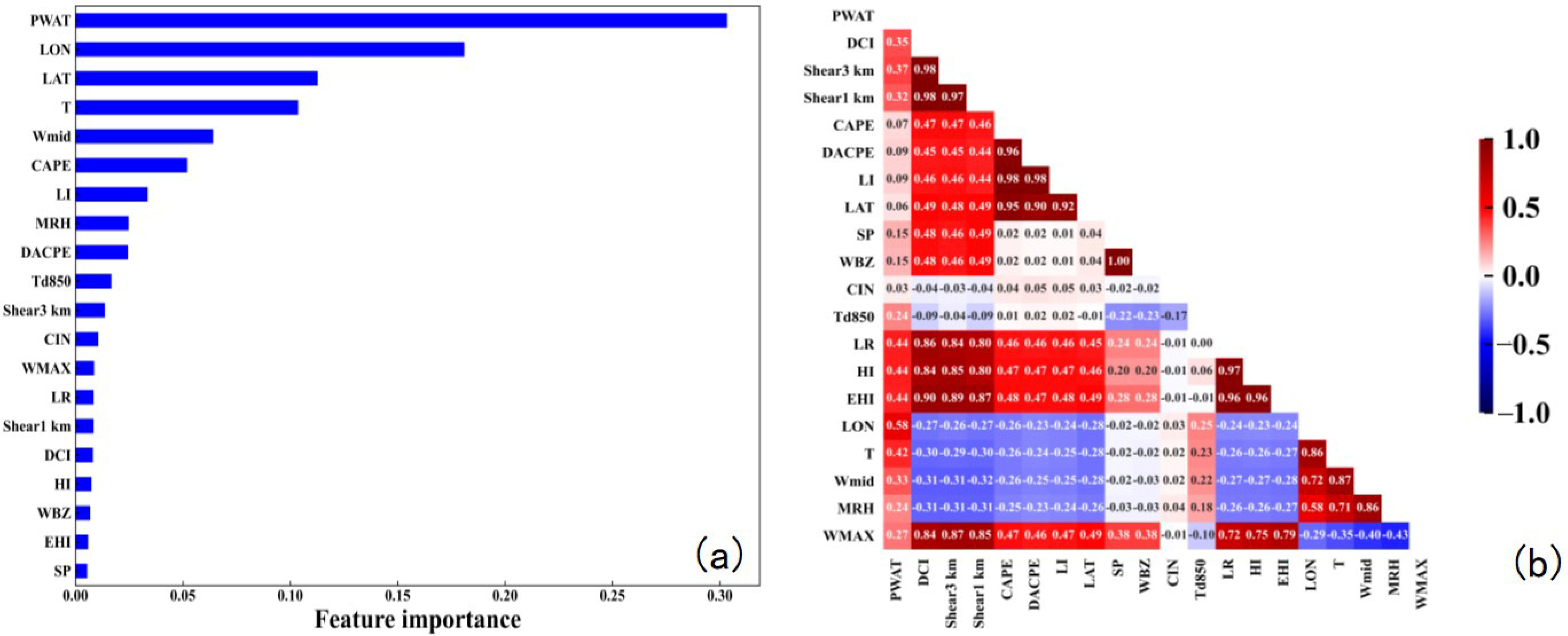
We employed the RF algorithm to assess the significance of forecasting variables within the training dataset, thereby determining the relative importance and correlation coefficients of each forecasting factor (see Figure 8). The results distinctly illustrate the critical role of moisture conditions in forecasting severe convective weather phenomena. The most significant variable identified was precipitable water (PWAT), which demonstrated markedly greater importance than the second most influential factor. Additionally, geographic location plays a substantial role in severe convective weather, with longitude (LON) ranking second and latitude (LAT) ranking third among all pertinent factors. Given that convective weather is primarily influenced by temperature, which causes near-surface air to heat, expand, and decrease in density, this process creates an unstable atmosphere conducive to the development of convective weather. Consequently, the temperature at 2 m above ground level (T) is recognized as the fourth most significant feature. The presence of strong convection requires specific atmospheric dynamic lifting conditions, with the average of vertical velocities (Wmid) positioned fifth. While atmospheric energy conditions do have some impact on severe convective weather, they are not the primary determinants; convective available potential energy (CAPE) ranks sixth, and the Lifted Index (LI) ranks seventh in terms of significance. These findings are consistent with the analyses conducted by forecasters on various types of convective weather, which take into account moisture, energy, dynamics, and other factors [56,57,58,59]. This highlights the exceptional capability of machine learning to autonomously extract relevant features and affirms the suitability of the sample dataset utilized.

4.3. Investigation of Reducing the Input Variables

A substantial number of meteorological datasets may occasionally be unavailable due to the failure of potential equipment quality issues in different places, which makes it difficult to use the best feasible input combinations derived in Section 2.1. Therefore, in this section, we examine the CNN-BiLSTM-AM model’s performance in the event that the ideal combination fails to exist. First, we examine how factor reduction affects the CNN-BiLSTM-AM model’s accuracy. We investigated the consequences of removing the most significant meteorological factors (i.e., PWAT, LON, LAT, T, and Wmid) successively on the precision of CNN-BiLSTM-AM. The findings are shown in

Table 4. Factor elimination analysis and CNN-BiLSTM-AM model’s accuracy on the testing dataset upon the loss of optimum combination. The values in parentheses represent the increase in RMSE after removing the specific factor compared to RMSE before the factor is removed. RMSE expressed in units of mm.

Factors Eliminated	RMSE
Wmid	11.43 (+0.32)
T	11.57 (+0.46)
LAT	11.38 (+0.17)
LON	11.70 (+0.59)
PWAT	13.09 (+1.98)

, which demonstrates that there were varying magnitudes of variation in the CNN-BiLSTM-AM model’s accuracy as a result of the removal of several meteorological elements during the testing phase. For instance, the findings indicated that the model’s performance became worse once Wmid was eliminated from the study, with the RMSE increasing from 11.11 mm to 11.43 mm. Our findings imply that in order to attain the best forecast accuracy, it is necessary to take into account both the advantages and disadvantages of ML-based models as well as the ideal input components.

4.4. Evaluation of the Model’s Capabilities across Various Scenarios in Bosten Lake Area

The Bosten Lake area is located in the southern foothills of the Tianshan Mountains in Xinjiang, China, situated to the northeast of the Tarim Basin and the southeast of the Yanqi Basin. It is blocked to the north by the Central Tianshan Mountains, bordered to the west by the Hohlar Mountains, and to the south by a branch of the South Tianshan Mountains—the Kuruktag Mountains. Being far from the ocean and deep inland, it serves as a transitional zone for the climate between northern and southern Xinjiang. The unique geographical location and topographical environment of the Bosten Lake area determine its arid and low-precipitation climate characteristics. During the summer, sudden heavy rain and localized convective weather often occur in the region, significantly impacting the lives and property of local residents. Due to the relatively low frequency of heavy precipitation events, previous studies have rarely focused on the heavy precipitation processes in such remote areas. Therefore, using this model to forecast severe convective weather in the Bosten Lake area is of great significance for ensuring the safety of the lives and property of the local population and for sustainable development.

As shown in

Table 5. Evaluation of CNN-BiLSTM-AM (DL) forecasts and human forecasts (HFs) for severe convective weather events from 2020 to 2022 in Bosten Lake area.

SCW	Year	POD (DL)	POD (HF)	$\mathbf{T}\mathbf{S}$ (DL)	TS (HF)
Short-term heavy precipitation	2020	0.545	0.426	0.465	0.403
	2021	0.532	0.401	0.453	0.392
	2022	0.501	0.411	0.472	0.407
Thunderstorm	2020	0.522	0.412	0.460	0.405
	2021	0.511	0.405	0.419	0.401
	2022	0.536	0.481	0.442	0.391
Hailstorm	2020	0.513	0.431	0.451	0.402
	2021	0.509	0.452	0.435	0.389
	2022	0.535	0.451	0.441	0.387
Strong gust	2020	0.492	0.422	0.430	0.383
	2021	0.476	0.433	0.468	0.402
	2022	0.483	0.442	0.455	0.395

, compared to the subjective forecasts of meteorologists, the CNN-BiLSTM-AM model has improved forecasting performance for various types of severe convective weather. For instance, the average TS score for short-term heavy rainfall reached 0.463, which is an improvement of 15.46% over the human forecasts’ score of 0.401; the average TS score for thunderstorms exceeded 0.440, representing an average increase of 10.28% compared to human forecasts; and the average TS scores for hailstorm and strong gust also improved by 12.47% and 14.76%, respectively, compared to human forecasts. From the above analysis, it can be concluded that the CNN-BiLSTM-AM model performs better in forecasting short-term heavy rainfall, thunderstorms, hail, and strong winds.

4.5. Possibility of Presenting the Model as a Universal Software Package

Presenting the CNN-BiLSTM-AM model as a universal software package entails packaging the model and its associated components in a user-friendly format that can be easily deployed and utilized by a wide range of users. Here are some considerations to explain the possibility of presenting the CNN-BiLSTM-AM model as a universal software package: (1) Ensure that the CNN-BiLSTM-AM model architecture is well-documented and modular, allowing for easy integration into a software package. Clear documentation will help users understand the model’s structure and functionalities. (2) Design the software package to be scalable, enabling users to train the model on different datasets and adapt it to various applications and use cases. Consider incorporating features that support scalability, such as batch processing and distributed computing. (3) Develop a user-friendly interface for the software package that allows users to interact with the model easily. Consider including visualization tools, input data preprocessing functionalities, and options for model customization. (4) Ensure that the software package is compatible with different operating systems and programming languages to maximize its accessibility and usability for a diverse user base. Provide clear instructions for installation and setup. (5) Include tools for model evaluation and performance metrics within the software package to help users assess the model’s accuracy and make informed decisions about its use in specific scenarios. (6) Provide comprehensive documentation and user guides to assist users in understanding the software package’s functionalities and capabilities. Offer technical support and resources for troubleshooting and assistance. (7) Implement version control mechanisms to track changes, updates, and improvements to the software package. Regularly release updates and patches to enhance the model’s performance and address any issues.

By addressing these considerations and developing a well-designed, user-friendly software package for the CNN-BiLSTM-AM model, it is possible to present the model as a universal tool that can be easily deployed and utilized by a broad audience for various weather forecasting and prediction tasks.

5. Conclusions

This research introduces a deep learning (DL) framework, designated as CNN-BiLSTM-AM, which integrates ERA5 hourly datasets alongside observational records to facilitate accurate forecasting of severe convective weather conditions. A comprehensive evaluation of the model’s performance is also conducted. To further elucidate the principles underlying convective weather forecast, we detail the training process while emphasizing the importance of predictive variables. The principal findings are as follows:

(1)

The CNN-BiLSTM-AM model demonstrates superior capabilities in identifying and interpreting complex nonlinear characteristics associated with severe convective weather systems when compared to traditional DL models such as LSTM, CNN, FC-LSTM, Predrnn++, and ConvLSTM. This results in a notable enhancement in precipitation forecast accuracy, particularly as the forecast lead time increases.

(2)

During the flood season, the CNN-BiLSTM-AM consistently outperforms alternative models in terms of root mean square error (RMSE), mean absolute error (MAE), Probability of Detection (POD), Threat Score (TS), and overall accuracy, thereby illustrating its effectiveness in addressing nonlinear challenges and delivering outstanding application results. However, it is noteworthy that the CNN-BiLSTM-AM exhibits a higher False Alarm Rate (FAR) relative to other models, which may suggest that while it accurately predicts precipitation events, it may also incorrectly forecast precipitation in scenarios where none is present.

(3)

The analysis of the significance of forecasting variables for severe convective weather reveals that precipitable water (PWAT) is the most critical moisture indicator, significantly surpassing the second-ranked feature. Geographical factors are also pivotal, with longitude (LON) and latitude (LAT) occupying the second and third positions, respectively. Given that temperature variations are fundamental to the causes of convective weather, the 2 m temperature (T) is identified as the fourth most influential factor. The necessity for atmospheric dynamic lifting conditions to promote strong convection positions average vertical velocities (Wmid) in fifth place. While atmospheric energetic conditions do influence severe convective weather, they are not the most critical, with convective available potential energy (CAPE) ranked sixth and the Lifted Index (LI) seventh.

Based on methods such as CNN, BiLSTM, and AM, a severe convective weather forecasting model called CNN-BiLSTM-AM has been developed, which significantly improves the accuracy of severe convective weather forecasts. By using the method of ranking the importance of forecasting factors, the model identifies the significance of each predictive factor, further deepening the understanding of the “black box” principle of deep learning models in forecasting severe convective weather. However, due to the scarcity of samples for heavy rain events and the serious imbalance issue, we need to adopt various approaches to expand the sample size. For example, we can use real-time recognition technology to increase the number of valid samples, employ data augmentation techniques to enhance the training set, and apply various machine learning methods to address the sample imbalance problem, such as transfer learning and custom loss functions. All of these methods require extensive experimentation and research work. Additionally, to explain the deep learning model and its predictions, we still need to conduct a lot of work, especially in using visualization techniques for deep learning to carry out interpretative research. Only in this way can we further enhance the credibility of deep learning methods, increase forecasters’ trust in the product, and expand its application scope.

References

1. Han, H.; Lee, S.; Im, J.; Kim, M.; Lee, M.; Ahn, M.; Chung, S. Detection of Convective Initiation Using Meteorological Imager Onboard Communication, Ocean, and Meteorological Satellite Based on Machine Learning Approaches. Remote Sens. 2015, 7, 9184–9204. [Google Scholar] [CrossRef]
2. Zheng, Y.; Zhou, K.; Sheng, J.; Lin, Y.; Tian, F.; Tang, W.; Lan, Y.; Zhu, W. Advances in Techniques of Monitoring, Forecasting and Warning of Severe Convective Weather. J. Appl. Meteorol. Sci. 2015, 26, 641–657. [Google Scholar]
3. Wang, X.; Mao, W.; Guo, J. Statistics features of strong convection weather disaster in China in 2004 main flood period. J. Nat. Disasters 2007, 16, 27–30. (In Chinese) [Google Scholar]
4. Zheng, Y.; Tian, F.; Meng, Z.; Xue, M.; Yao, D.; Bai, L.; Zhou, X.; Mao, X.; Wang, M. Survey and Multi Scale Characteristics of Wind Damage Caused by Convective Storms in the Surrounding Area of the Capsizing Accident of Cruise Ship “Dongfangzhixing”. Meteorol. Mon. 2016, 42, 1–13. (In Chinese) [Google Scholar]
5. Zheng, Y.; Zhu, W.; Yao, D.; Meng, Z.; Xue, M.; Zhao, K.; Wu, Z.; Wang, X.; Zheng, Y. Wind Speed Scales and Rating of the Intensity of the 23 June 2016 Tornado in Funing County, Jiangsu Province. Meteorol. Mon. 2016, 42, 1289–1303. (In Chinese) [Google Scholar]
6. Gao, Z.; Zhang, J.; Yu, M.; Liu, Z.; Yin, R.; Zhou, S.; Zong, L.; Ning, G.; Xu, X.; Guo, Y. Role of water vapor modulation from multiple pathways in the occurrence of a record-breaking heavy rainfall event in China in 2021. Earth Space Sci. 2022, 9, e2022EA002357. [Google Scholar] [CrossRef]
7. Quenum, G.M.L.D.; Arnault, J.; Klutse, N.A.B.; Zhang, Z.; Kunstmann, H.; Oguntunde, P.G. Potential of the Coupled WRF/WRF-Hydro Modeling System for Flood Forecasting in the Ouémé River (West Africa). Water 2022, 14, 1192. [Google Scholar] [CrossRef]
8. Varlas, G.; Papadopoulos, A.; Papaioannou, G.; Dimitriou, E. Evaluating the Forecast Skill of a Hydrometeorological Modelling System in Greece. Atmosphere 2021, 12, 902. [Google Scholar] [CrossRef]
9. Giannaros, C.; Dafis, S.; Stefanidis, S.; Giannaros, T.M.; Koletsis, I.; Oikonomou, C. Hydrometeorological analysis of a flash flood event in an ungauged Mediterranean watershed under an operational forecasting and monitoring context. Meteorol. Appl. 2022, 29, e2079. [Google Scholar] [CrossRef]
10. Kryza, M.; Werner, M.; Waszek, K.; Dore, A.J. Application and evaluation of the WRF model for high-resolution forecasting of rainfall—A case study of SW Poland. Meteorol. Z. 2013, 22, 595–601. [Google Scholar] [CrossRef]
11. Hamill, T.M. Performance of Operational Model Precipitation Forecast Guidance during the 2013 Colorado Front-Range Floods. Mon. Weather Rev. 2012, 142, 2609–2618. [Google Scholar] [CrossRef]
12. Sela, J.G. Spectral modeling at the National Meteorological Center. Mon. Weather Rev. 1980, 108, 1279–1292. [Google Scholar] [CrossRef]
13. Juang, H.M.H. A reduced spectral transform for the NCEP seasonal forecast global spectral atmospheric model. Mon. Weather Rev. 2004, 132, 1019–1035. [Google Scholar] [CrossRef]
14. Juang, H.M.H. Mass conserving positive definite semi-Lagrangian advection in NCEP GFS: Decomposition of massively parallel computing without halo. In Proceedings of the 13th Workshop on Use of High Performance Computing in Meteorology, Reading, UK, 3–7 November 2008; ECMWF: Reading, UK, 2008; p. 50. [Google Scholar]
15. Eckermann, S. Hybrid σ–p coordinate choices for a global model. Mon. Weather Rev. 2009, 137, 224–245. [Google Scholar] [CrossRef]
16. Yang, F. On the negative water vapor in the NCEP GFS: Sources and solution. In Proceedings of the 23rd Conference in Weather Analysis and Forecasting/19th Conference on Numerical Weather Prediction, Omaha, NE, USA, 1–5 June 2009. [Google Scholar]
17. Juang, H.M.H. A spectral fully compressible nonhydrostatic mesoscale model in hydrostatic sigma coordinates: Formulation and preliminary results. Meteorol. Atmos. Phys. 1992, 50, 75–88. [Google Scholar] [CrossRef]
18. Weisman, M.L.; Skamarock, W.C.; Klemp, J.B. The resolution dependence of explicitly modeled convective systems. Mon. Weather Rev. 1997, 125, 527–548. [Google Scholar] [CrossRef]
19. Done, J.; Davis, C.A.; Weisman, M. The next generation of NWP: Explicit forecasts of convection using the Weather Research and Forecasting (WRF) Model. Atmos. Sci. Lett. 2004, 5, 110–117. [Google Scholar] [CrossRef]
20. Roberts, N.M.; Lean, H.W. Scale-selective verification of rainfall accumulations from highresolution forecasts of convective events. Mon. Weather Rev. 2008, 136, 78–97. [Google Scholar] [CrossRef]
21. Prein, A.F.; Langhans, W.; Fosser, G.; Ferrone, A.; Ban, N.; Goergen, K.; Keller, M.; Telle, M.; Gutjahr, O.; Feser, F.; et al. A review on regional convection-permitting climate modeling: Demonstrations, prospects, and challenges. Rev. Geophys. 2015, 53, 323–361. [Google Scholar] [CrossRef]
22. Stevens, B.; Bony, S. What are climate models missing? Science 2013, 340, 1053–1054. [Google Scholar] [CrossRef]
23. McGovern, A.; Elmore, K.L.; Gagne II, D.J.; Haupt, S.E.; Karstens, C.D.; Lagerquist, R.; Smith, T.; Williams, J.K. Using artificial intelligence to improve real-time decision-making for high-impact weather. Bull. Am. Meteorol. Soc. 2017, 98, 2073–2090. [Google Scholar] [CrossRef]
24. Reichstein, M.; Camps-Valls, G.; Stevens, B.; Jung, M.; Denzler, J.; Carvalhais, N. Deep learning and process understanding for data-driven Earth system science. Nature 2019, 566, 195–204. [Google Scholar] [CrossRef]
25. Li, W.J.; Zhao, F.; Li, M.J.; Chen, L.; Peng, X. Forecasting and Classification of Severe Convective Weather Based on Numerical Forecast and Random Forest Algorithm. Meteorol. Mon. 2018, 44, 49–58. (In Chinese) [Google Scholar]
26. Herman, G.R.; Schumacher, R.S. Money Doesn’t Grow on Trees, but Forecasts Do: Forecasting Extreme Precipitation with Random Forests. Mon. Weather Rev. 2018, 146, 1571–1600. [Google Scholar] [CrossRef]
27. Liu, N.N.; Liu, C.T.; Tissot, P.E. A Bayesian-Like Approach to Describe the Regional Variation of High-Flash Rate Thunderstorms from Thermodynamic and Kinematic Environment Variables. Geophys. Res. Atmos. 2019, 124, 12507–12522. [Google Scholar] [CrossRef]
28. Krizhevsky, A.; Sutskever, I.; Hinton, G.E. Imagenet classification with deep convolutional neural networks. In Proceedings of the 25th International Conference on Neural Information Processing Systems; Curran Associates Inc.: Red Hook, NY, USA, 2012; pp. 1097–1105. [Google Scholar]
29. LeCun, Y.; Bengio, Y. Convolutional networks for images, speech, and time series. In The Handbook of Brain Theory and Neural Networks; Arbib, M.A., Ed.; MIT Press: Cambridge, MA, USA, 2019; pp. 255–258. [Google Scholar]
30. Szegedy, C.; Toshev, A.; Erhan, D. Deep neural networks for object detection. In Proceedings of the 26th International Conference on Neural Information Processing Systems; Curran Associates Inc.: Red Hook, NY, USA, 2013; pp. 2553–2561. [Google Scholar]
31. Lin, T.Y.; Li, Q.Y.; Geng, Y.A.; Jiang, L. Attention-Based Dual-Source Spatiotemporal Neural Network for Lightning Forecast. IEEE Access 2019, 7, 158296–158307. [Google Scholar] [CrossRef]
32. Gope, S.; Sarkar, S.; Mitra, P.; Ghosh, S. Early Prediction of Extreme Rainfall Events: A Deep Learning Approach. In Advances in Data Mining; Springer: Berlin/Heidelberg, Germany, 2016. [Google Scholar]
33. Bi, K.; Xie, L.; Zhang, H.; Chen, X.; Gu, X.; Tian, Q. Accurate medium-range global weather forecasting with 3D neural networks. Nature 2023, 619, 533–538. [Google Scholar] [CrossRef]
34. Lam, R.; Sanchez-Gonzalez, A.; Willson, M.; Wirnsberger, P.; Fortunato, M.; Alet, F.; Ravuri, S.; Ewalds, T.; Eaton-Rosen, Z.; Hu, W.; et al. Learning skillful medium-range global weather forecasting. Science 2023, 382, 1416–1421. [Google Scholar] [CrossRef]
35. Hersbach, H.; Bell, B.; Berrisford, P.; Hirahara, S.; Horanyi, A.; MuñozSabater, J.; Nicolas, J.; Peubey, C.; Radu, R.; Schepers, D.; et al. The ERA5 global reanalysis. Q. J. R. Meteorol. Soc. 2020, 146, 1999–2049. [Google Scholar] [CrossRef]
36. Smith, B.T.; Thompson, R.L.; Grams, J.S.; Broyles, C.; Brooks, H.E. Convective modes for significant severe thunderstorms in the contiguous United States. Part I: Storm classification and climatology. Weather Forecast. 2012, 27, 1114–1135. [Google Scholar] [CrossRef]
37. Brooks, H.E. Severe thunderstorms and climate change. Atmos. Res. 2013, 123, 129–138. [Google Scholar] [CrossRef]
38. Madhulatha, A.; Rajeevan, M.; Ratnam, M.V.; Bhate, J.; Naidu, C.V. Nowcasting severe convective activity over Southeast India using ground-based microwave radiometer observations. J. Geophys. Res. 2013, 118, 1–13. [Google Scholar] [CrossRef]
39. Gascon, E.; Merino, A.; Sanchez, J.L.; Fernandez-Gonzalez, S.; García-Ortega, E.; Lopez, L.; Hermida, L. Spatial distribution of thermodynamic conditions of severe storms in southwestern Europe. Atmos. Res. 2015, 164, 194–209. [Google Scholar] [CrossRef]
40. Púčik, T.; Groenemeijer, P.; Rýva, D.; Kolař, M. Proximity soundings of severe and nonsevere thunderstorms in Central Europe. Mon. Weather Rev. 2015, 143, 4805–4821. [Google Scholar] [CrossRef]
41. Gijben, M.; Dyson, L.L.; Loots, M.T. A statistical scheme to forecast the daily lightning threat over southern Africa using the unified model. Atmos. Res. 2017, 194, 78–88. [Google Scholar] [CrossRef]
42. Taszarek, M.; Brooks, H.E.; Czernecki, B. Sounding-derived parameters associated with convective hazards in Europe. Mon. Weather Rev. 2017, 145, 1511–1528. [Google Scholar] [CrossRef]
43. Ukkonen, P.; Mäkelä, A. Evaluation of machine learning classifiers for predicting deep convection. J. Adv. Model. Earth Syst. 2019, 11, 1784–1802. [Google Scholar] [CrossRef]
44. Krawczyk, B. Learning from imbalanced data: Open challenges and future directions. Prog. Artif. Intell. 2016, 5, 221–232. [Google Scholar] [CrossRef]
45. Buda, M.; Maki, A.; Mazurowski, M.A. Systematic study of the class imbalance problem in convolutional neural networks. arXiv 2017, arXiv:1710.05381. [Google Scholar] [CrossRef]
46. Lu, W.J.; Li, J.Z.; Wang, J.Y.; Qin, L. A CNN-BiLSTM-AM method for stock price predictiona. Neural Comput. Appl. 2021, 33, 4741–4753. [Google Scholar] [CrossRef]
47. Kingma, D.; Ba, J.A. A Method for Stochastic Optimization. In Proceedings of the International Conference on Learning Representations (ICLR), Banff, AB, Canada, 14–16 April 2014. [Google Scholar]
48. Perol, T.; Gharbi, M.; Denolle, M. Convolutional Neural Network for Earthquake Detection and Location. Sci. Adv. 2017, 4, 2–10. [Google Scholar] [CrossRef] [PubMed]
49. Shi, X.; Chen, Z.; Wang, H.; Yeung, D.Y.; Wong, W.K.; Woo, W.C. Convolutional LSTM network: A machine learning approach for precipitation nowcasting. Adv. Neural Inf. Process. Syst. 2015, 28, 802–810. [Google Scholar]
50. Wang, Y.; Wu, H.; Zhang, J.; Gao, Z.; Wang, J.; Yu, P.S.; Long, M. PredRNN: A Recurrent Neural Network for Spatiotemporal Predictive Learning. IEEE Trans. Pattern Anal. Mach. Intell. 2023, 45, 2208–2225. [Google Scholar] [CrossRef]
51. Zhou, K.H.; Zheng, Y.G.; Li, B.; Dong, W.S.; Zhang, X.L. Forecasting different types of convective weather: A deep learning approach. J. Meteorol. Res. 2019, 33, 797–809. [Google Scholar] [CrossRef]
52. Kim, S.; Hong, S.; Joh, M.; Song, S.K. DEEPRAIN: ConvLSTM network for precipitation prediction using multichannel radar data. In Proceedings of the 7th International Workshop on Climate Informatics, National Center for Atmospheric Research, Boulder, CO, USA, 19–22 September 2017. [Google Scholar]
53. Akbari Asanjan, A.; Yang, T.; Hsu, K.; Sorooshian, S.; Lin, J.; Peng, Q. Short-Term Precipitation Forecast Based on the PERSIANN System and LSTM Recurrent Neural Networks. J. Geophys. Res. Atmos. 2018, 123, 12–543. [Google Scholar] [CrossRef]
54. Skamarock, W.C.; Klemp, J.B.; Dudhia, J.; Gill, D.O.; Liu, Z.; Berner, J.; Wang, W.; Powers, J.G.; Duda, M.G.; Barker, D.; et al. A Description of the Advanced Research WRF Model Version 4 (Vol. 145); National Center for Atmospheric Research: Boulder, CO, USA, 2019. [Google Scholar]
55. McGovern, A.; Lagerquist, R.; Gagne, D.J., II.; Jergensen, G.E.; Elmore, K.L.; Homeyer, C.R.; Smith, T. Making the black box more transparent: Understanding the physical implications of machine learning. Bull. Am. Meteorol. Soc. 2019, 100, 2175–2199. [Google Scholar] [CrossRef]
56. Tian, F.; Zheng, Y.; Zhang, T.; Zhang, X.; Mao, D.; Sun, J.; Zhao, S. Statistical characteristics of environmental parameters for warm season short-duration heavy rainfall over central and eastern China. Meteorol. Res. 2015, 29, 370–384. [Google Scholar] [CrossRef]
57. Zeng, Y.; Yang, L.M. Analysis on Mesoscale Impact System and Atmospheric Vertical Structure of Two Types of Heavy Rains in Urumqi. Plateau Meteorol. 2020, 39, 774–787. [Google Scholar]
58. Zhang, F.; Li, G.; Luo, X. Some Influence Factors of a Sudden Rainstorm Event in Northeast Sichuan Basin of China. Plateau Meteorol. 2020, 39, 321–332. [Google Scholar]
59. Zhang, J.; Gao, Z.; Yang, J.; Li, Y.; Jiang, Y. Research and Numerical Simulation of Rainstorm over Bosten Lake Area based on WRF Model. Plateau Meteorol. 2022, 41, 887–895. [Google Scholar]
Figure 1. The flowchart of the proposed model.
Atmosphere 15 01229 g001
Figure 2. The research area chosen for the study (the white box represents Henan); shaded areas represent topographical features distribution (unit: m).
Atmosphere 15 01229 g002
Figure 3. Scattered density plots of various DL models on the testing dataset (a): FC-LSTM, (b): ConvLSTM, (c): Predrnn++, (d): CNN, (e): CNN-BiLSTM-AM, and (f): LSTM).
Atmosphere 15 01229 g003
Figure 4. Taylor plots from six models.
Atmosphere 15 01229 g004
Figure 5. RMSE distribution of FC-LSTM (a), ConvLSTM (b), Predrnn++ (c), CNN (d), CNN-BiLSTM-AM (e), and LSTM (f) in Henan on 22 July 2022.
Atmosphere 15 01229 g005
Figure 6. TS score for convective weather event on 22 July 2022 (the red line is the CNN-BiLSTM-AM model score, and the green line is the WRF score).
Atmosphere 15 01229 g006
Figure 7. Assessment of precipitation histograms predicted by six models across various months: (a) denotes RMSE, (b) denotes FAR, (c) denotes MAR, (d) denotes POD, (e) denotes TS, and (f) denotes ACCURACY.
Atmosphere 15 01229 g007
Figure 8. Feature importance (a) and correlation coefficients (b) of each forecast factor.
Atmosphere 15 01229 g008