Article

Development of Machine Learning and Deep Learning Prediction Models for PM2.5 in Ho Chi Minh City, Vietnam

by
Phuc Hieu Nguyen
1,2,*,
Nguyen Khoi Dao
1,2 and
Ly Sy Phu Nguyen
1,2
1
Faculty of Environment, University of Science, Ho Chi Minh City 700000, Vietnam
2
Vietnam National University, Ho Chi Minh City 700000, Vietnam
*
Author to whom correspondence should be addressed.
Atmosphere 2024, 15(10), 1163; https://doi.org/10.3390/atmos15101163
Submission received: 14 August 2024 / Revised: 19 September 2024 / Accepted: 26 September 2024 / Published: 29 September 2024
(This article belongs to the Special Issue Atmospheric Pollution in Highly Polluted Areas)

Abstract

:
The application of machine learning and deep learning in air pollution management is becoming increasingly crucial, as these technologies enhance the accuracy of pollution prediction models, facilitating timely interventions and policy adjustments. They also facilitate the analysis of large datasets to identify pollution sources and trends, ultimately contributing to more effective and targeted environmental protection strategies. Ho Chi Minh City (HCMC), a major metropolitan area in southern Vietnam, has experienced a significant rise in air pollution levels, particularly PM2.5, in recent years, creating substantial risks to both public health and the environment. Given the challenges posed by air quality issues, it is essential to develop robust methodologies for predicting PM2.5 concentrations in HCMC. This study seeks to develop and evaluate multiple machine learning and deep learning models for predicting PM2.5 concentrations in HCMC, Vietnam, utilizing PM2.5 and meteorological data over 911 days, from 1 January 2021 to 30 June 2023. Six algorithms were applied: random forest (RF), extreme gradient boosting (XGB), support vector regression (SVR), artificial neural network (ANN), generalized regression neural network (GRNN), and convolutional neural network (CNN). The results indicated that the ANN is the most effective algorithm for predicting PM2.5 concentrations, with an index of agreement (IOA) value of 0.736 and the lowest prediction errors during the testing phase. These findings imply that the ANN algorithm could serve as an effective tool for predicting PM2.5 concentrations in urban environments, particularly in HCMC. This study provides valuable insights into the factors that affect PM2.5 concentrations in HCMC and emphasizes the capacity of AI methodologies in reducing atmospheric pollution. Additionally, it offers valuable insights for policymakers and health officials to implement targeted interventions aimed at reducing air pollution and improving public health.

1. Introduction

Air pollution is a significant global issue, particularly in urban areas, where both short-term and long-term exposure to polluted air can have severe health consequences [1]. Among the various air pollutants, particulate matter with a diameter of 2.5 microns or smaller (PM2.5) is of particular concern. PM2.5’s diminutive size enables it to infiltrate the respiratory system, resulting in significant health issues, including respiratory and cardiovascular disorders, and potentially premature mortality [2]. Environmental pollution remains a major global health threat, with recent estimates from 2018 indicating that nine out of ten individuals inhale air that contains elevated levels of pollutants [3]. Both ambient and household air pollution contribute to approximately seven million deaths globally each year, with around 2.2 million of these deaths occurring in the Western Pacific Region alone. In Vietnam, air pollution is accountable for an estimated 60,000 deaths annually [3].
Ho Chi Minh City (HCMC), one of Vietnam’s largest and fastest expanding urban hubs, has experienced a notable rise in air pollution levels in recent years. This increase is primarily driven by metropolitan expansion, industrial growth, and a surge in road traffic [4]. As per a report from GreenID, in the three years 2016, 2017, and 2018, the air quality index (AQI) results reveal a troubling trend, as the percentage of AQI readings categorized as unhealthy escalated from 31.1% in 2016 to 41.9% in 2017, and subsequently to 44.2% in 2018 [5]. The declining air quality in HCMC has emerged as a critical issue for politicians, health officials, and the general populace. This issue has led to increased healthcare costs and economic burdens, necessitating urgent actions such as stricter emissions regulations, public health campaigns, and community engagement to mitigate the adverse effects and improve overall air quality. Therefore, developing effective strategies to predict PM2.5 in HCMC is crucial.
Air pollutant concentration prediction models play a vital role in both assessing and managing air quality, offering critical insights for policymakers and environmental managers. These models are indispensable in optimizing air quality monitoring systems by providing detailed information on pollution levels, sources of pollutants, and the overall status of air quality in different regions [6]. By predicting future pollution levels, decisionmakers can take proactive measures such as issuing early warnings, implementing public health campaigns, or enforcing stricter emission regulations to mitigate adverse environmental and health impacts. The ability to forecast air quality at specific future points allows for better preparedness and more informed decision making regarding pollution control strategies [7].
There are two primary types of PM2.5 concentration prediction models: knowledge-driven models and data-driven models. Knowledge-driven models, such as chemical transport models, are based on atmospheric science and require a thorough understanding of pollutant emission sources, transport mechanisms, and chemical transformations in the atmosphere. These models simulate the diffusion, transmission, and cross-regional transport of pollutants, making them highly valuable for detailed atmospheric analysis. However, they are often computationally intensive, requiring precise input data and extensive computational resources. Additionally, the complexity of atmospheric interactions and uncertainties in emission inventories can limit the accuracy of these models, particularly when dealing with real-world data that may not be as well structured as experimental conditions. In contrast, data-driven models are more practical and have become increasingly popular due to their ability to handle large datasets and generate predictions based on data characteristics. These models, which rely on statistical methods or machine learning techniques, are often more flexible and less dependent on detailed atmospheric knowledge. Data-driven approaches can be classified into three groups: statistical models, artificial intelligence (AI) models, and hybrid models that combine elements of both. AI models, in particular, have gained significant attention in recent years, driven by advancements in computational power and the Fourth Industrial Revolution. These models are known for their high accuracy and reliability in air quality prediction, as they excel at modeling complex, nonlinear phenomena and relationships between numerous exogenous variables [8]. One of the key strengths of AI-based models is their ability to process vast amounts of data rapidly, offering significant advantages in terms of processing speed, scalability, and cost-effectiveness. AI models, such as machine learning and deep learning techniques, have the capability to impute missing data, identify hidden patterns in large datasets, and generate accurate predictions of pollution levels at specific future points. Moreover, AI models can provide spatial and temporal predictions, allowing researchers to estimate pollution levels for particular areas and times with a high degree of precision [9]. In addition to their ability to simulate air quality, AI techniques also allow for real-time monitoring and adaptive learning, further enhancing their effectiveness in dynamic environments.
Numerous studies have proven the effectiveness of AI models in predicting air quality, specifically PM2.5 levels. For example, Bingyue Pan (2018) employed the XGBoost algorithm to predict PM2.5 levels in Tianjin City [10], whereas Zamani et al. (2019) applied random forest, XGBoost, and deep learning methodologies utilizing multiplatform remote sensing information to forecast PM2.5 levels in Tehran [11]. Goulier et al. (2020) provided an hourly forecast of ten atmospheric pollutant levels in Münster utilizing an artificial neural network (ANN) methodology [12], whereas Castelli et al. (2020) employed support vector regression (SVR) to anticipate pollutant and particle levels in California [13]. Likewise, Gou et al. (2020) utilized statistical correlation evaluation and ANNs to discern relationships among the air pollution index and weather variables in Xi’an and Lanzhou [14]. Doreswamy et al. (2020) created machine learning models to forecast PM levels of the atmospheric conditions of Taiwan [15]. In the U.S., Zhou et al. (2020) examined several machine learning methodologies employed for air pollution prediction, with applications that span multiple regions, including high-pollution urban areas [16]. Similarly, Chen et al. (2020) investigated how climate change influences PM2.5 levels, using multimodel projections to assess the effectiveness of predictive models in the U.S [17]. In Europe, Ordóñez et al. (2020) utilized multimodel simulations combined with machine learning techniques to improve air quality predictions, particularly for PM2.5 levels, while Petetin et al. (2020) developed high-resolution forecasting models to enhance predictive accuracy across the continent [18,19]. In China, Zheng et al. (2021) employed deep learning models to enhance the accuracy of PM2.5 concentration predictions, showcasing the latest advancements in air quality modeling [20]. These recent studies underscore the global applicability of machine learning in tackling air pollution and provide a strong foundation for the methods employed in this paper for HCMC.
In HCMC, PM2.5 data are not very available, with limited research focusing on predicting PM2.5 levels. Few studies are currently available that predict these concentrations. Vo et al. (2021) applied WRF model to predict PM2.5 level in HCMC [21]. Their study aimed to evaluate the prediction of PM2.5 concentration by predicting meteorological variables using the WRF model. In addition to utilizing a limited number of meteorological factors (four variables), their study did not thoroughly address the optimization of input scenarios. Another study from Rajnish et al. (2023) built a multivariate model for predicting air quality, taking into account diverse factors like meteorological circumstances, air quality metrics, and urban spatial data, and time factors to forecast NO2, SO2, O3, and CO hourly concentrations [22]. This research attained a significant achievement in forecasting using spatially scattered data; however, the duration of data collection was relatively short, spanning only from February to December 2021. Additionally, data utilized in this investigation were gathered from monitoring stations associated with a specific research project, rather than from official, reliable, and publicly accessible government sources.
The primary objective of this research is to develop and evaluate various machine learning and deep learning algorithms for predicting PM2.5 concentrations in HCMC, using meteorological and PM2.5 data. The results from this study are expected to enhance the comprehension of the determinants affecting PM2.5 levels in this metropolis and underscore the potential of AI methodologies in alleviating air pollution and promoting public health.

2. Methodology

This section delineates the methods utilized for prediction of PM2.5 levels in HCMC using various machine learning and deep learning algorithms. The establishment of a PM2.5 prediction model has five key steps (Figure 1): (1) Data processing, (2) analyzing the impact of parameters on PM2.5, (3) designing scenarios of input datasets, (4) modeling machine learning and deep learning algorithms to predict PM2.5, and (5) selecting the best prediction model for PM2.5 among the developed machine learning and deep learning prediction models (Figure 1).
Firstly, daily data over 911 days, from 1 January 2021 to 30 June 2023, including meteorological and PM2.5 parameters in HCMC, were collected for the development of a prediction model. The meteorological data included ambient temperature, relative humidity, wind speed, rainfall, sunshine hours, and evaporation that were collected from Tan Son Hoa weather station (10.79723° N, 106.6667° E) at 236B Le Van Sy, Tan Binh District, while the PM2.5 data were obtained from the monitoring station at the U.S Consulate (10.7831° N, 106.7001° E) at 4 Le Duan street in District 1 in HCMC. These two stations are about 4 km apart as the crow flies and about 5 km apart by road. The collected data were then processed by removing unavailable data points and outliers.
Secondly, the processed data were analyzed to determine feature importance and identify the impact of the examined parameters on the objective function.
Thirdly, different sets of input data were generated to develop machine learning-based prediction models.
Fourthly, various machine learning and deep learning algorithms, including RF, XGB, SVR, ANN, GRNN, and CNN, were employed to formulate predictive models for PM2.5 in HCMC. Each algorithm employed in this work presents a distinct methodology for addressing the intricacies of PM2.5 prediction, providing varied advantages in feature selection, model training, and predictive accuracy. To evaluate the performance of these models, the dataset was split into training and testing sets. Specifically, 80% of the data were allocated for training, while the remaining 20% were designated for testing to evaluate model performance. For deep learning algorithms such as ANN and CNN, which require a validation set to monitor model training and prevent overfitting, the training data were further divided. In this case, 80% of the training data were used as sub-training data, and 20% of the training data were used for validation. This approach ensured that model training could be halted when validation performance began to decline, reducing the risk of overfitting. The remaining 20% of the dataset was consistently used as the testing set across all models to provide a final evaluation of prediction accuracy.
Random forest, often known as RF, is a type of ensemble learning technique that works by creating a vast ensemble of decision trees through the training process and then displaying the average forecast of each individually constructed tree [23]. Its ensemble structure renders it highly resilient to overfitting. The program initiates the process by generating a randomized dataset derived from the primary data. For every bootstrapped sample, a decision tree is built by selecting the best split from a randomly chosen subset of features at every node. The bootstrap aggregation technique generates multiple bootstrap samples through sampling and replacement, from which decision trees are constructed. The ultimate prediction is the mean of the forecasts from all individual trees [24]. This study selects RF to predict PM2.5 levels due to its superior performance across several domains, resilience to overfitting, and efficacy in situations characterized by highly nonlinear and complex relationships between features and target variables. The performance of the RF model can be regulated by tuning hyperparameters including the quantity of trees in the forest, the depth of the trees, the minimum samples required for a split, the minimum samples required for a leaf node, and the maximum possible leaf nodes [25].
XGBoost is a powerful and scalable ensemble learning method widely used for regression and classification problems. It improves on traditional gradient boosting by optimizing the handling of regularization and model optimization [26]. This work employs XGB to forecast PM2.5 values by using its capacity to simulate intricate linkages and interactions in the dataset. The algorithm processes historical air quality and meteorological data, which enables it to discern patterns that affect PM2.5 concentrations. XGB possesses numerous hyperparameters that could be adjusted to enhance performance, such as the learning rate, the ensemble size, the tree depth, the sample size for each tree, and the feature count for each tree [27].
Support vector regression (SVR) is a type of machine learning algorithm used for regression tasks, which is derived from the support vector machine (SVM) framework [28]. Support vector regression (SVR) is recognized for its capacity to manage high-dimensional data and to represent nonlinear relationships via kernel functions [29]. It develops a model by transforming input data into a higher-dimensional space to facilitate linear regression analysis. SVR seeks to identify a function that diverges from the actual observed objectives by no more than a defined margin ϵ, while simultaneously maintaining maximal flatness. This study utilizes SVR to forecast PM2.5 concentrations in HCMC by training the model using atmospheric quality and meteorological data. The hyperparameters in SVR comprise the regularization parameter C, the epsilon ϵ that delineates the margin of tolerance, and the parameters linked to the selected kernel function, such as the kernel coefficient γ for the radial basis function kernel.
Artificial neural networks (ANNs) are a category of machine learning techniques designed to emulate the architecture and functionality of the human brain [23,30]. An artificial neural network consists of several interconnected processing nodes, or neurons, that collaboratively execute intricate computations. The method processes a collection of input data via multiple hidden layers to obtain an output. Each neuron within the network takes input from neurons in the preceding layer and use an activation function to generate an output [31]. The output from each neuron is subsequently transmitted to the neurons in the subsequent layer, and this process is reiterated until the output layer is reached. The design of the network, comprising the quantity of layers and the number of neurons per layer, can be tailored to improve efficiency for a certain task. Training ANNs entails modifying weights and biases of neurons to reduce a loss function, which quantifies the disparity between the expected output and observed output [30]. This process is generally executed by backpropagation that entails calculating the gradient of the loss function concerning the weights and biases, subsequently employing it to adjust the network’s parameters. Utilizing the adaptability and efficacy of learning intricate and nonlinear relationships among variables, ANNs are employed to predict PM2.5 levels by training the network on atmospheric conditions data, atmospheric condition datasets, and other pertinent aspects. The model acquires the ability to discern intricate patterns and relationships in the data that affect PM2.5 values. An optimum artificial neural network design consists of a configuration of hyperparameters, such as the quantity of hidden layers, the quantity of neurons in each hidden layer, activation function, learning rate, weight constraints, and dropout rate, which produce the most accurate predictions on the validation data.
Generalized regression neural networks (GRNNs) [32] are a category of artificial neural networks grounded in nonparametric predictive modeling. GRNNs are recognized for their rapid training capabilities and proficiency in modeling intricate correlations between input and target variables [33]. GRNNs comprise four layers: the input layer, pattern layer, summation layer, and output layer. Each neuron in the pattern layer denotes a training example and computes a distance metric to the input. These distances are consolidated by the summation layer, which produces weighted outputs. The output layer delivers a predicted value derived from these consolidated data. The fundamental principle of GRNNs is the application of kernel regression to approximate the conditional expectation of the output variable based on the input parameter. It utilizes a radial basis function to evaluate the probability density of data points and generates predictions based on the weighted aggregation of these functions. GRNNs are adept at managing noisy and intricate datasets, making them well suited for predicting air quality, particularly PM2.5 concentrations, which are influenced by numerous factors. The smoothing parameter (σ) is a hyperparameter in GRNNs. The performance of the model is highly sensitive to the value of σ, with smaller values potentially resulting in overfitting, while larger values may lead to underfitting.
A convolutional neural network (CNN) is a form of deep learning model that integrates several layers including convolutional, pooling, and fully connected layers. Convolutional layers utilize filters on input data to identify characteristics, such as edges or textures, via convolution processes. The dimensionality of data is reduced by pooling layers, which utilize maximum pooling to preserve significant features while reducing computational demands. The fully linked layers at the network’s conclusion integrate these features to generate final predictions. CNNs excel in managing large-scale and high-dimensional data, making them suitable for predicting PM2.5 levels. The convolutional layers assist in recognizing critical characteristics and trends influencing PM2.5 values. To improve the efficacy of the CNN model, essential hyperparameters like the quantity and dimensions of convolutional filters, the depth of layers, the learning rate, and the batch size will be systematically maximized. Each best-performing model is tuned to its optimal hyperparameters using a grid search method. The range for each hyperparameter is detailed in the results section for each machine learning algorithm. Optimal hyperparameters are determined using the validation dataset. This optimization process aims to find the hyperparameters that yield the minimal root mean square error (RMSE) on the validation set.
Finally, after evaluating the predictive outcomes of the constructed models, the best-performing model is selected for PM2.5 prediction in HCMC. In this study, the prediction models are evaluated using various metrics, including root mean square error (RMSE), mean absolute percentage error (MAPE), index of agreement (IOA), and normalized mean bias (NMB). These evaluation metrics are expressed as follows:
R M S E = 1 n i = 1 n y i y ^ i 2
M A P E = 100 n i = 1 n y i y ^ i y i
I O A = 1 i = 1 n ( y i y ^ i ) 2 i = 1 n ( y ^ i y ¯ + y i y ¯ ) 2
N M B = i = 1 n ( y ^ i y i ) i = 1 n y i
where n is the total number of data points; y ¯ is the mean of the actual observed values; y i and y ^ i are the actual observed value and predicted value for the ith data point, respectively; RMSE measures the square root of the average squared variances between predicted and observed values; and MAPE evaluates the mean absolute percentage error between forecasted and actual values. Furthermore, the IOA quantifies the extent of model prediction inaccuracy on a scale from 0 to 1, with 1 signifying perfect concordance and 0 denoting complete discordance. IOA is formulated to address certain constraints of the coefficient of determination by offering a normalized metric of model prediction error. It considers the disparities between the anticipated and observed values, providing a more balanced measure of model performance, especially in cases with nonlinear relationships or when dealing with outliers. On the other hand, NMB measures the average discrepancy between the anticipated and observed values, normalized by the means of the observed values. It indicates the bias of the model’s predictions. Values approaching 0 signify little bias, whereas positive values denote overestimation and negative values signify underestimating.

3. Experimentation and Results

3.1. General Statistics of Data

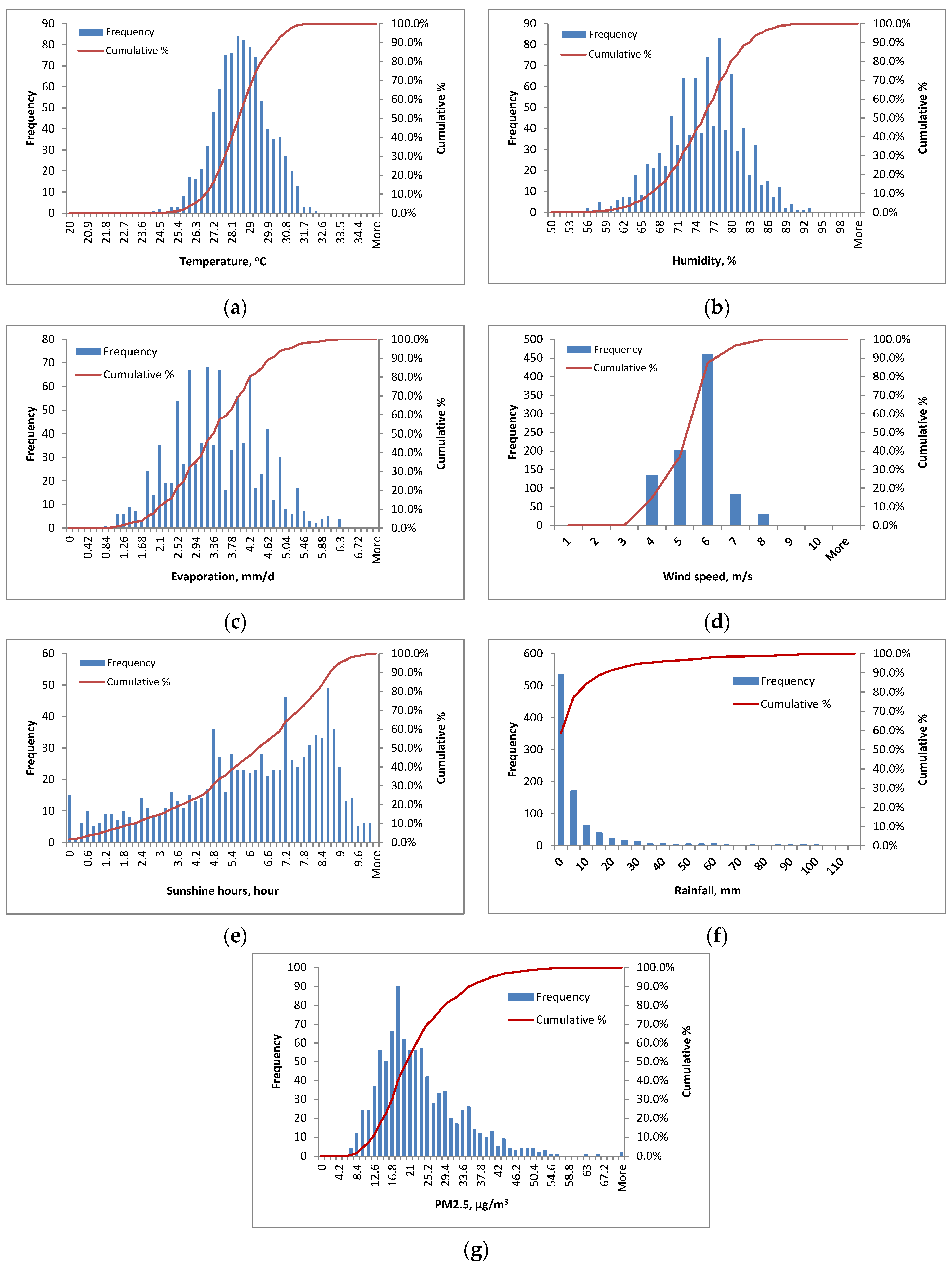
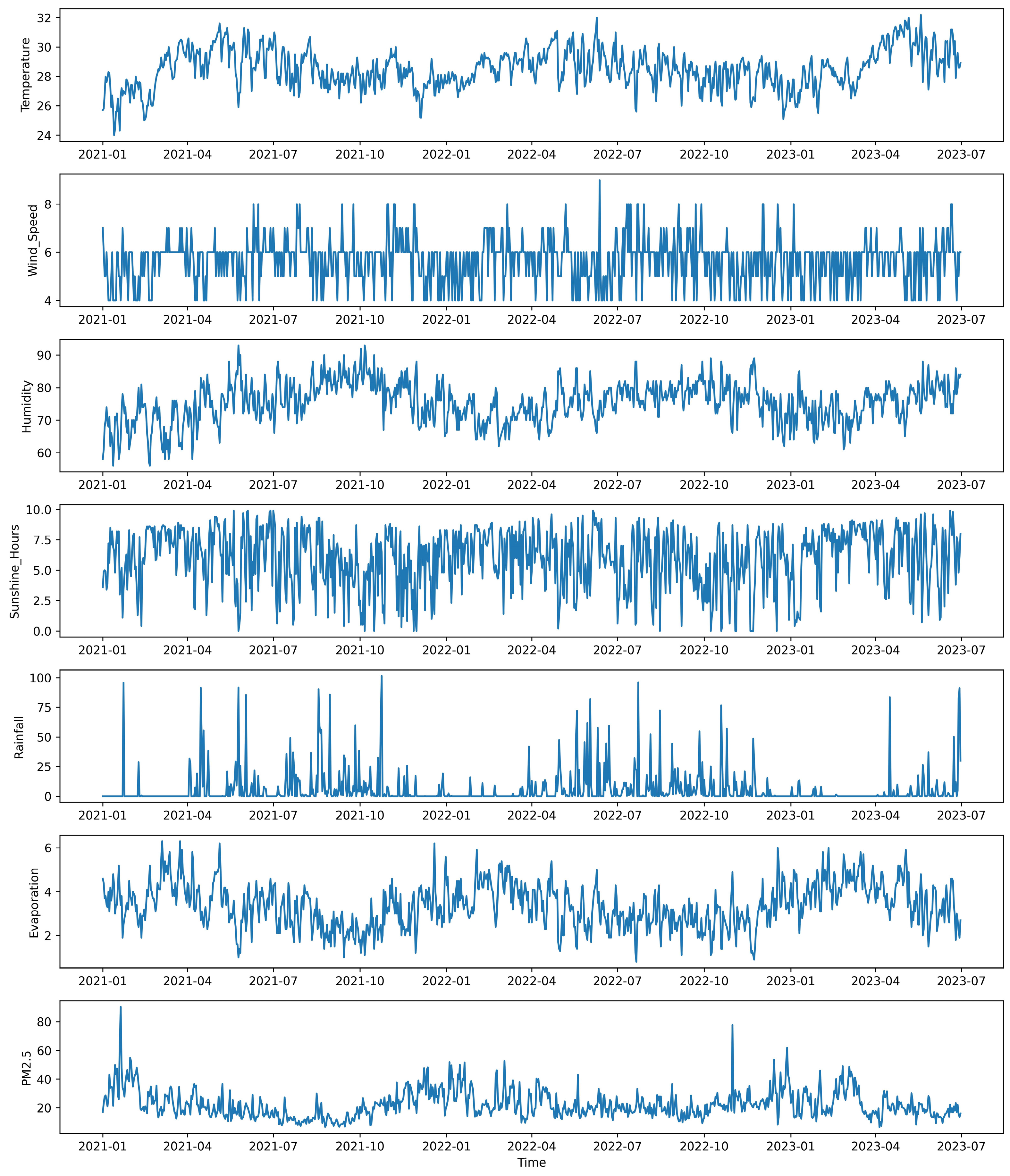
The meteorological data and PM2.5 levels collected in HCMC between 2021 and 2023 are presented in Figure 2, illustrating the seasonal fluctuations of climatic variables and PM2.5 levels. In total, the dataset contains 911 days of data across seven parameters, which were used for model training, testing, and validation. HCMC has a dry season from December to April, favored for its sunny weather, and a rainy season from May to November, marked by high humidity and frequent heavy rainfalls [34]. The rainy season accounts for about 80–90% of the city’s annual rainfall, with the heaviest downpours typically occurring between June and August [35]. Additionally, temperature, sunshine hours, and evaporation are high during the dry season and low during the rainy season. Conversely, rainfall, humidity, and wind speed are high in the rainy season and reduced during the dry season. Moreover, PM2.5 concentrations tend to be higher during the dry season compared to the rainy season. The fundamental statistics of the data were shown in Table 1 and the distributions were shown in Figure 3.
To provide a comprehensive overview of the data characteristics, Table 1 presents the summary statistics of the meteorological factors and PM2.5 concentrations. The purpose of this table is to illustrate the variability and distribution of the data, offering key insights into the range and central tendency of each feature. For instance, temperature varied between 24.0 °C and 32.2 °C, and wind speed ranged from 0.0 to 9.0 m/s, highlighting the diverse meteorological conditions during the study period. These variations are critical to understanding how the models interpret and process the input data, as fluctuations in weather patterns are expected to influence PM2.5 levels. Table 1 provides the foundation for assessing how these features individually and collectively impact air quality. Figure 2 and Figure 3 further complement the information in Table 1 by visualizing the temporal distribution and variability of the meteorological parameters and PM2.5 concentrations. Figure 2 illustrates different environmental and meteorological data trends from January 2021 to July 2023. Furthermore, Figure 3 shows the distribution of each feature, which helps to identify any skewness, outliers, or anomalies in the data. Together, these figures enhance our understanding of the temporal and distributional characteristics of the dataset.

3.2. Feature Selection

To construct suitable and optimal prediction scenarios, this study analyzed the correlation between meteorological values and PM2.5 concentrations, identifying the relationships among these parameters to propose scenarios based on the correlation analysis results. Table 2 shows the correlation between the meteorological parameters and PM2.5 concentration in HCMC. The Pearson correlation coefficient (r) was employed to determine the degree of correlation between the input variables and PM2.5 concentrations. This coefficient ranges from −1 to 1, with values close to 1 indicating a strong positive correlation, values close to −1 indicating a strong negative correlation, and values around 0 indicating little or no linear correlation.
The results showed that humidity, temperature, and wind speed have a strong correlation with PM2.5, while rainfall, evaporation, and sunshine hours have a moderate correlation with PM2.5.
Different scenarios of input parameters were generated to develop prediction models. This allows us to evaluate the prediction performance under various sets of input parameters. These scenarios were designed based on the Pearson correlation coefficient obtained from the previous step. In this approach, scenarios were constructed by prioritizing the most correlated parameters down to the less correlated ones [36,37]. Starting with the highest correlation coefficient, each scenario incrementally incorporated additional parameters in descending order of their correlation. This stepwise approach allowed for an exploration of how the predictive power of the models evolved as features of varying correlation were sequentially integrated into the input data, providing insights into the cumulative effect of features on the model’s predicting performance, aiding in the effective optimization and selection of input parameters. The input feature scenarios are detailed in Table 3.

3.3. Development of Prediction Models

3.3.1. Random Forest Model

This section details the development of a random forest algorithm designed to predict PM2.5 concentrations based on many input scenarios detailed in Table 3. The model was trained using various hyperparameters featuring n_estimators, max_depth, min_samples_split, min_samples_leaf, and max_leaf_nodes, as detailed in Table 4.
The random forest model demonstrated strong predictive capabilities, achieving IOA values between 0.361 and 0.789 on the training set and 0.396 to 0.670 on the testing set under all scenarios (Table 5). Generally, the inclusion of more input features improved the accuracy in predicting PM2.5 concentration. In addition, the model achieved relatively low RMSE, MAPE, and NMB values, indicating its effectiveness in accurately predicting PM2.5 concentrations under each scenario.
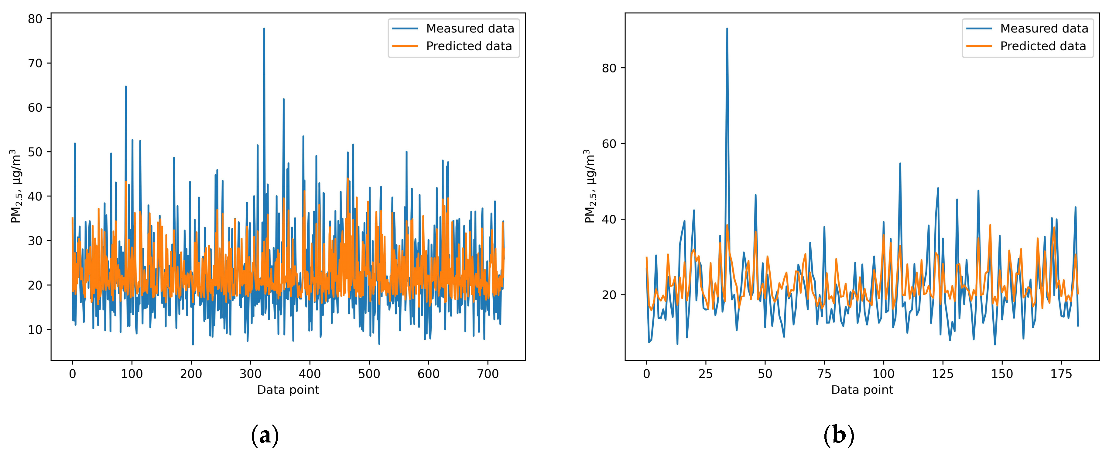
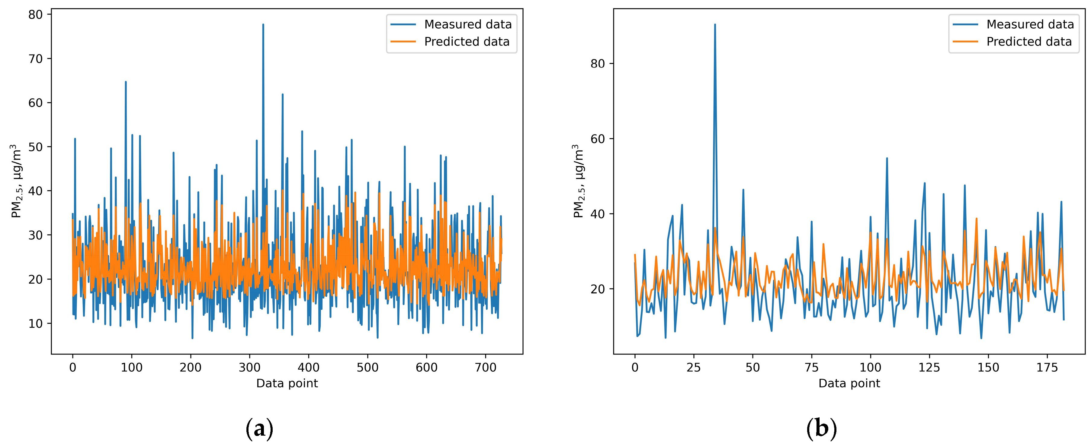
The highest prediction accuracy was achieved with input scenario 6, which resulted in high IOA values and relatively low RMSE, MAPE, and NMB values for training and testing evaluation. This indicates that the model is well fitted and capable of reliably predicting PM2.5 concentrations based on the given input variables. The optimal model was configured with an n_estimators of 1500, a max_depth of 12, a min_samples_split of 4, a min_samples_leaf of 5, and max_leaf_nodes set to 90. Figure 4 illustrates the training and testing results of this optimized random forest model, showing moderate agreement between predicted and actual PM2.5 values, which suggests a reasonably strong predictive performance.

3.3.2. XGB Model

This section discusses the development and performance analysis of an XGB algorithm aimed at predicting PM2.5 concentrations using the input scenarios outlined in Table 3. The models were trained and optimized by fine-tuning the hyperparameters listed in Table 6.
The training and testing results across different scenarios are summarized in Table 7, demonstrating moderate model performance. IOA values ranged from 0.302 to 0.740 during training and from 0.320 to 0.687 during testing. The model achieved the best predictive accuracy using input scenario 5, which included variables including humidity, temperature, wind speed, rainfall, and evaporation. However, adding more input features did not significantly enhance prediction accuracy.
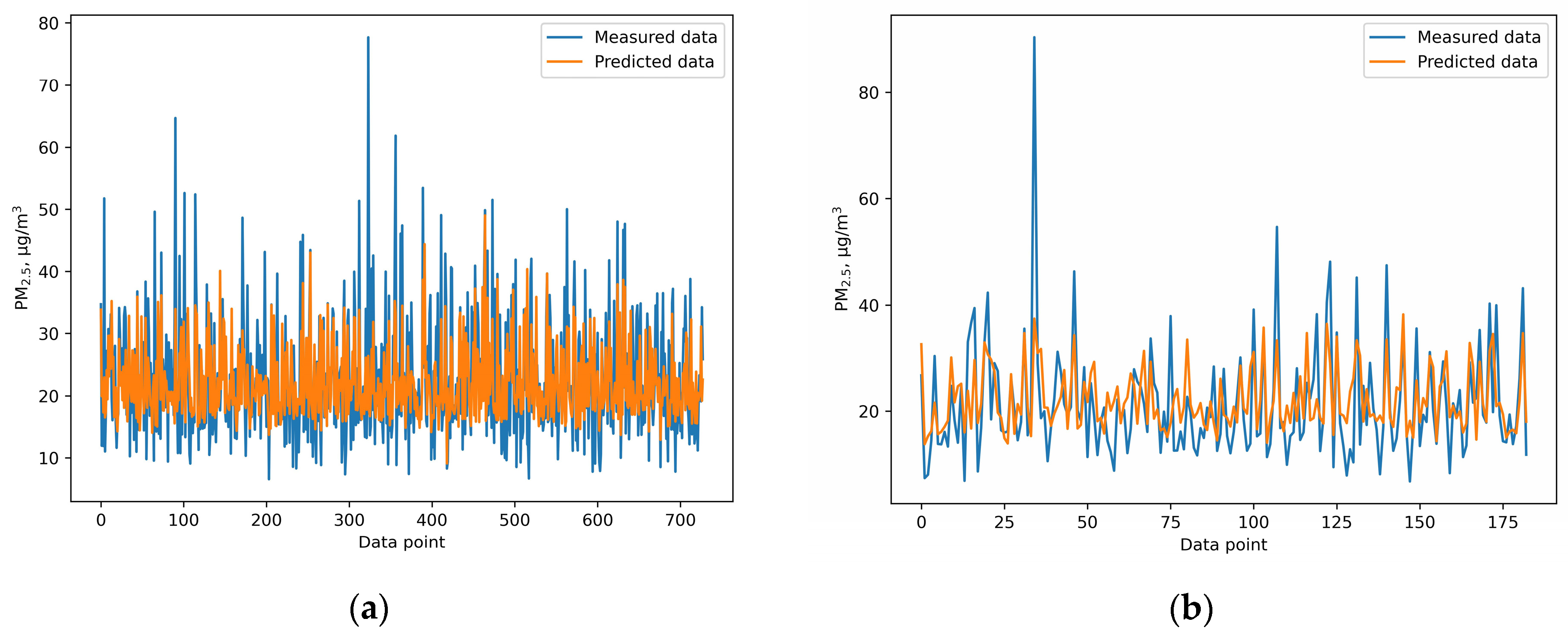
The optimal XGB model was obtained with hyperparameters including an n_estimators of 10,000, a max_depth of 3, a learning rate of 0.0005, a subsample of 0.5, a colsample_bytree of 0.8, and a min_child_weight of 3. The training and testing results of this optimal model are depicted in Figure 5, which illustrates moderate alignment between predicted and observed PM2.5 values, confirming the model’s satisfactory predictive ability.

3.3.3. Support Vector Regression Model

This section details the development and evaluation of an SVR algorithm for predicting PM2.5 concentrations, using the input scenarios provided in Table 3. The models were fine-tuned by adjusting the hyperparameters shown in Table 8.
The performance results across various scenarios are summarized in Table 9, where the model showed moderate effectiveness. IOA values ranged from 0.322 to 0.720 during training and from 0.361 to 0.709 during testing. The highest accuracy was obtained using input scenario 5, which included factors like humidity, temperature, wind speed, rainfall, and evaporation.
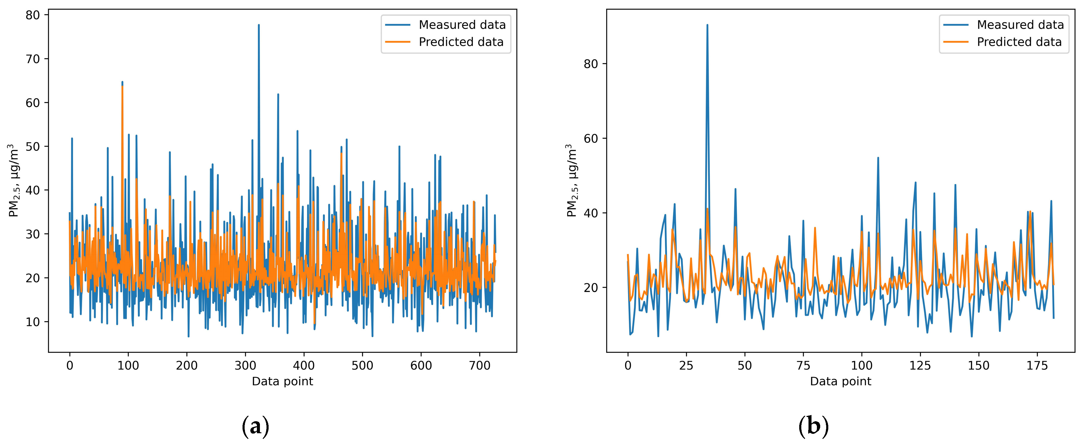
The optimal SVR model was configured with the following hyperparameters: a radial basis function (rbf) kernel, C set to 1.0, epsilon at 0.1, and gamma set to scale. Figure 6 presents training and testing results of this optimal model, which showed strong agreement between predicted and actual PM2.5 values, indicating a solid predictive capability.

3.3.4. Artificial Neural Network Model

This section discusses the application of an ANN algorithm to predict PM2.5 concentrations based on each input scenario. The hyperparameters of the model, such as the quantity of hidden layers, the number of neurons in each hidden layer, the activation function, learning rate, dropout rate, and weight constraint, were optimized, with their ranges detailed in Table 10.
Table 11 summarizes training results and testing results, which indicate strong performance of ANN model in both phases, with high IOA values and relatively low values of RMSE, MAPE, and NMB. During training, IOA values ranged from 0.357 to 0.713, suggesting the model effectively captures data variability. Testing results showed similar trends, with IOA values between 0.328 and 0.736, further supporting the model’s robustness.
Scenario 6 exhibited the best performance, with the highest IOA and the lowest RMSE, MAPE, and NMB values for both training and testing datasets. Consequently, the model developed using input scenario 6, and hyperparameters specified in Table 12, was identified as the optimal ANN model. Figure 7 illustrates the training and testing outcomes of this model, showing a strong alignment between predicted and measured PM2.5 values, confirming its reliable predictive capability.

3.3.5. Generalized Regression Neural Network Model

This section presents the development and assessment of a GRNN algorithm to predict PM2.5 concentrations, based on the input scenarios described in Table 3. The models were trained and optimized by fine-tuning the hyperparameters listed in Table 13.
The performance of the GRNN model, summarized in Table 14, ranged from moderate to high, with IOA values between 0.344 and 0.785 for training and between 0.372 and 0.695 for testing. The highest prediction accuracy was observed in scenario 6, which included all input features.
The optimal GRNN model was configured with rbf kernel and a sigma of 0.111. Figure 8 illustrates the training and testing results of this optimized model, showing moderate agreement between predicted and actual PM2.5 values, confirming its moderate predictive capability.

3.3.6. Convolutional Neural Network Model

This section discusses the development and evaluation of a CNN model designed to predict PM2.5 concentrations using the input scenarios specified in Table 3. The models were trained and optimized by adjusting the hyperparameters outlined in Table 15.
The training and testing results across different scenarios, summarized in Table 16, showed that the model’s performance ranges from moderate to high. IOA values were between 0.396 and 0.581 for training, and between 0.437 and 0.607 for testing. The model achieved the highest accuracy using scenario 6, which incorporated all input features. Overall, increasing the number of input parameters generally led to improved accuracy, with scenario 6 yielding the best performance.
The optimal CNN model was configured using 192 convolutional filters, a kernel size of 1, a tanh activation function, 128 neurons in a fully connected layer, a dropout rate of 0.0, and a learning rate of 0.0006. Figure 9 illustrates the training and testing outcomes of this optimized model, showing moderate agreement between predicted and observed PM2.5 values, which suggests the model’s satisfactory predictive capability.

3.3.7. Selection of Prediction Model for PM2.5 in HCMC, Vietnam

Within the scope of this investigation, six distinct machine learning methods were utilized to forecast the PM2.5 concentration: random forest, XGB, SVR, ANN, GRNN, and CNN. The predictive capabilities of each model were evaluated on various input scenarios, with performance compared in terms of IOA, RMSE, MAPE, and NMB for both training and testing datasets.
Among all models, the ANN algorithm emerged as the top performer, achieving the highest IOA value of 0.736 and the lowest RMSE, MAPE, and NMB values of 7.978, 32.452, and 4.8726, respectively (Table 17). The SVR algorithm demonstrated solid performance, achieving an IOA of 0.709 and relatively low error metrics. However, the ANN model consistently outperformed the SVR across all evaluation metrics.
Building on these findings, the ANN model was ultimately selected as the optimal predictive model for this particular PM2.5 dataset. Its higher IOA value and lower error metrics for testing sets suggest that ANN outperforms the other assessed models. Consequently, the trained ANN model was selected for predicting PM2.5 concentrations in HCMC, Vietnam.

4. Discussion

This study provides a comprehensive comparison of the performance of six different machine learning and deep learning algorithms, random forest, XGB, SVR, ANN, GRNN, and CNN, in predicting PM2.5 concentrations. Additionally, meteorological variables including temperature, humidity, wind speed, sunshine hours, rainfall, and evaporation were included to enhance the prediction accuracy. Among the models, the ANN model outperformed the others, achieving an IOA of 0.736, an RMSE of 7.978, and an NMB of 0.032 during the testing phase. These findings highlight the effectiveness of machine learning techniques in air quality prediction and highlight the importance of selecting an appropriate algorithm for predicting air pollution. This study provides valuable insights for health officials and policymakers by demonstrating that machine learning models, especially the ANN model, can accurately predict PM2.5 concentrations. This insight is valuable for policymakers, as it can inform the implementation of effective strategies to mitigate health risks associated with PM2.5 exposure. For instance, our model could enable authorities to issue air quality alerts when PM2.5 levels are expected to rise above safe thresholds. This allows citizens to take precautionary measures, such as staying indoors or using masks on high-risk days. In addition, public health campaigns can be timed based on pollution predictions, informing residents of exposure risks and protective actions like wearing air filters or limiting outdoor activities.
Despite the promising results, this study has several limitations that should be addressed in future research. First, this study concentrates exclusively on PM2.5 levels in HCMC. A more comprehensive comprehension of air quality throughout the nation would be achieved by broadening the scope to include additional communities in Vietnam. Additionally, while machine learning and deep learning methods were applied to simulate and predict PM2.5 concentrations, the study was limited by the availability of data from a single automatic monitoring station—the U.S. Consulate station in HCMC. Consequently, the results primarily reflect PM2.5 concentration levels within the vicinity of the consulate. A larger number of standard automatic monitoring stations would enable a more generalized and representative analysis of the entire study area.
Furthermore, this study focused on predicting PM2.5 concentrations based on meteorological factors, but PM2.5 concentrations are also influenced by various other factors, such as emission sources and the presence of other air pollutants. Emission sources, including industrial zones, construction sites, and high-traffic areas, are closely related to PM2.5 concentrations. Factors such as the relative location and proximity of these sources to monitoring stations significantly impact dust concentrations. Additionally, the concentrations of other air pollutants, such as NOx, SOx, CO2, and H2S, may interact with PM2.5 concentrations. Due to data limitations, these parameters were not included in this study. Future research should find the effect of these pollutants on PM2.5 concentrations and consider integrating them into prediction models.
This study establishes a robust basis for subsequent research on PM2.5 predictions for HCMC, and its findings can contribute to the development of effective air pollution control and management strategies.

5. Conclusions

This study investigated the prediction of PM2.5 concentrations in HCMC utilizing six distinct machine learning and deep learning algorithms. The models were trained and validated on a dataset including temperature, humidity, wind speed, sunshine hours, rainfall, and evaporation. Among the algorithms assessed, the ANN showed superior performance in predicting PM2.5 levels, achieving an IOA of 0.736 and the lowest RMSE, MAPE, and NMB values during testing. These results highlight the potential of machine learning algorithms, particularly ANNs, in accurately predicting PM2.5 concentrations based on meteorological data. The implications of this research are significant for HCMC, where air pollution poses a critical public health concern. By utilizing these predictive models, policymakers and health officials can implement more targeted and effective interventions to mitigate air pollution, ultimately improving public health outcomes. This study advocates for the integration of advanced machine learning techniques into environmental monitoring systems, offering a framework for proactive urban air quality management.

Author Contributions

Conceptualization, N.K.D. and P.H.N.; methodology, P.H.N.; software, P.H.N.; validation, N.K.D. and P.H.N.; formal analysis, L.S.P.N.; investigation, L.S.P.N.; resources, L.S.P.N.; data curation, P.H.N.; writing—review and editing, P.H.N.; visualization, P.H.N.; supervision, L.S.P.N.; project administration, P.H.N. All authors have read and agreed to the published version of the manuscript.

Funding

This research received no external funding.

Institutional Review Board Statement

Not applicable.

Informed Consent Statement

Not applicable.

Data Availability Statement

The data presented in this study are available on request from the corresponding author. The data are not publicly available due to privacy.

Acknowledgments

I would like to express my deepest gratitude to my late supervisor, Dao Nguyen Khoi, whose guidance, support, and expertise were invaluable throughout this research project. His dedication to the field and his unwavering commitment to excellence have left a lasting impact on my work and personal growth. This work would not have been possible without his mentorship and encouragement. He will be greatly missed and remembered fondly.

Conflicts of Interest

The authors declare no conflicts of interest.

References

  1. Usmani, R.S.A.; Saeed, A.; Abdullahi, A.M.; Pillai, T.R.; Jhanjhi, N.Z.; Hashem, I.A.T. Air Pollution and Its Health Impacts in Malaysia: A Review. Air Qual. Atmos. Health 2020, 13, 1093–1118. [Google Scholar] [CrossRef]
  2. Health and Environmental Effects of Particulate Matter (PM). Available online: https://www.epa.gov/pm-pollution/health-and-environmental-effects-particulate-matter-pm (accessed on 1 May 2024).
  3. WHO. Air Pollution in Viet Nam. Available online: https://www.who.int/vietnam/health-topics/air-pollution#:~:text=New estimates in 2018 reveal,million people die each year (accessed on 1 May 2024).
  4. Bang, H.Q.; Khue, V.H.N. Air Emission Inventory. In Air Pollution—Monitoring, Quantification and Removal of Gases and Particles; IntechOpen: London, UK, 2019; pp. 1–18. [Google Scholar] [CrossRef]
  5. Green Innovation and Development Center. Air Quality Report 2018 in Vietnam; Green Innovation and Development Center: Hanoi, Vietnam, 2019. [Google Scholar]
  6. Singh, D.; Dahiya, M.; Kumar, R.; Nanda, C. Sensors and Systems for Air Quality Assessment Monitoring and Management: A Review. J. Environ. Manag. 2021, 289, 112510. [Google Scholar] [CrossRef] [PubMed]
  7. Hung, M.D. Application of Machine Learning to Fill in the Missing Monitoring Data of Air Quality. Vietnam J. Sci. Technol. 2018, 56, 104–110. [Google Scholar] [CrossRef]
  8. López, M. Multivariate Statistical Machine Learning Methods for Genomic Prediction; Springer: Cham, Switzerland, 2022. [Google Scholar]
  9. Oyebode, O.; Stretch, D. Neural Network Modeling of Hydrological Systems: A Review of Implementation Techniques. Nat. Resour. Model. 2019, 32, e12189. [Google Scholar] [CrossRef]
  10. Pan, B. Application of XGBoost Algorithm in Hourly PM2.5 Concentration Prediction. IOP Conf. Ser. Earth Environ. Sci. 2018, 113, 012127. [Google Scholar] [CrossRef]
  11. Joharestani, M.Z.; Cao, C.; Ni, X.; Bashir, B.; Talebiesfandarani, S. PM2.5 Prediction Based on Random Forest, XGBoost, and Deep Learning Using Multisource Remote Sensing Data. Atmosphere 2019, 10, 373. [Google Scholar] [CrossRef]
  12. Goulier, L.; Paas, B.; Ehrnsperger, L.; Klemm, O. Modelling of Urban Air Pollutant Concentrations with Artificial Neural Networks Using Novel Input Variables. Int. J. Environ. Res. Public Health 2020, 17, 2025. [Google Scholar] [CrossRef]
  13. Castelli, M.; Clemente, F.M.; Popovič, A.; Silva, S.; Vanneschi, L. A Machine Learning Approach to Predict Air Quality in California. Complexity 2020, 2020, 049504. [Google Scholar] [CrossRef]
  14. Guo, Q.; He, Z.; Li, S.; Li, X.; Meng, J.; Hou, Z.; Liu, J.; Chen, Y. Air Pollution Forecasting Using Artificial and Wavelet Neural Networks with Meteorological Conditions. Aerosol Air Qual. Res. 2020, 20, 1429–1439. [Google Scholar] [CrossRef]
  15. Doreswamy; Harishkumar, K.S.; Km, Y.; Gad, I. Forecasting Air Pollution Particulate Matter (PM2.5) Using Machine Learning Regression Models. In Procedia Computer Science; Elsevier: Amsterdam, The Netherlands, 2020; Volume 171, pp. 2057–2066. [Google Scholar]
  16. Zhou, X.; Liu, J.; Zhang, X. Air Pollution Prediction Using Machine Learning Approaches: A Review. J. Clean. Prod. 2020. [Google Scholar]
  17. Chen, K.; Fiore, A.; Westervelt, D.M. The Influence of Climate Change on PM2.5 and Ozone in the United States: A Review of Multi-Model Projections. J. Air Waste Manag. Assoc. 2020, 70, 583. [Google Scholar]
  18. Ordóñez, C.; Mathis, H.; Friese, E.; Mues, A. Multi-Model Simulations and Machine Learning Techniques for Improving Air Quality Predictions. Atmospheric Chemistry and Physics. Atmos. Chem. Phys. 2020, 20, 84. [Google Scholar]
  19. Petetin, H.; Bowdalo, D.; Granell, C. Machine Learning Model for High Resolution PM2.5 Forecasting in Europe. Environ. Pollut. 2020, 266, 11518. [Google Scholar]
  20. Zheng, Y.; Wang, J.; Zhang, J. Deep Learning Models for Air Pollution Prediction and PM2.5 Analysis in China. Environ. Sci. Technol. 2021, 55, 422. [Google Scholar]
  21. Vo, T.T.M.; Tran, T.T.; To, T.H. PM2.5 Forecast System by Using Machine Learning and WRF Model, A Case Study: Ho Chi Minh City, Vietnam. Aerosol Air Qual. Res. 2021, 21, 210108. [Google Scholar] [CrossRef]
  22. Rakholia, R.; Le, Q.; Quoc Ho, B.; Vu, K.; Simon Carbajo, R. Multi-Output Machine Learning Model for Regional Air Pollution Forecasting in Ho Chi Minh City, Vietnam. Environ. Int. 2023, 173, 107848. [Google Scholar] [CrossRef]
  23. Müller, A.; Guido, S. Introduction to Machine Learning with Python: A Guide for Data Scientists, 1st ed.; O’Reilly Media: Sebastopol, CA, USA, 2016; ISBN 978-1449369415. [Google Scholar]
  24. Breiman, L. Random Forests. Mach. Learn. 2001, 45, 5–32. [Google Scholar] [CrossRef]
  25. Scikit-Learn Random Forest Regressor. Available online: https://scikit-learn.org/stable/modules/generated/sklearn.ensemble.RandomForestRegressor.html (accessed on 1 April 2024).
  26. Chen, T.; Guestrin, C. XGBoost. In Proceedings of the 22nd ACM SIGKDD International Conference on Knowledge Discovery and Data Mining, San Francisco, CA, USA, 13–17 August 2016; ACM: New York, NY, USA, 2016; pp. 785–794. [Google Scholar]
  27. XGBoost XGBoost Parameters. Available online: https://xgboost.readthedocs.io/en/stable/parameter.html (accessed on 1 May 2024).
  28. Platt, J. Probabilistic Outputs for Support Vector Machines and Comparisons to Regularized Likelihood Methods. 1999. Available online: https://home.cs.colorado.edu/~mozer/Teaching/syllabi/6622/papers/Platt1999.pdf (accessed on 1 May 2024).
  29. Piri, J.; Abdolahipour, M.; Keshtegar, B. Advanced Machine Learning Model for Prediction of Drought Indices Using Hybrid SVR-RSM. Water Resour Manag. 2023, 37, 683–712. [Google Scholar] [CrossRef]
  30. Géron, A. Hands-On Machine Learning with Scikit-Learn, Keras, and Tensor Flow: Concepts, Tools, and Techniques to Build Intelligent Systems, 2nd ed.; O’Reilly Media: Sebastopol, CA, USA, 2019; ISBN 978-1492032649. [Google Scholar]
  31. LeCun, Y.; Bengio, Y.; Hinton, G. Deep Learning. Nature 2015, 521, 436–444. [Google Scholar] [CrossRef]
  32. Specht, D.F. A General Regression Neural Network. IEEE Trans. Neural Netw. 1991, 2, 568–576. [Google Scholar] [CrossRef]
  33. Liu, K.; Lin, T.; Zhong, T.; Ge, X.; Jiang, F.; Zhang, X. New Methods Based on a Genetic Algorithm Back Propagation (GABP) Neural Network and General Regression Neural Network (GRNN) for Predicting the Occurrence of Trihalomethanes in Tap Water. Sci. Total Environ. 2023, 870, 161976. [Google Scholar] [CrossRef] [PubMed]
  34. Nguyen, T.N.T.; Du, N.X.; Hoa, N.T. Emission Source Areas of Fine Particulate Matter (PM2.5) in Ho Chi Minh City, Vietnam. Atmosphere 2023, 14, 579. [Google Scholar] [CrossRef]
  35. Hien, T.T.; Nguyen, L.S.P.; Truong, M.T.; Pham, T.D.H.; Ngan, T.A.; Minh, T.H.; Hau, L.Q.; Trung, H.T.; Nhon, N.T.T.; Nguyen, N.T. Spatiotemporal Variations of Atmospheric Mercury at Urban and Suburban Areas in Southern Vietnam Megacity: A Preliminary Year-Round Measurement Study. Atmos. Environ. 2024, 333, 120664. [Google Scholar] [CrossRef]
  36. Zhang, C.; Luo, Z.; Rezgui, Y.; Zhao, T. Enhancing Multi-Scenario Data-Driven Energy Consumption Prediction in Campus Buildings by Selecting Appropriate Inputs and Improving Algorithms with Attention Mechanisms. Energy Build. 2024, 311, 114133. [Google Scholar] [CrossRef]
  37. Nguyen-Le, V.; Shin, H.; Chen, Z. Deep Neural Network Model for Estimating Montney Shale Gas Production Using Reservoir, Geomechanics, and Hydraulic Fracture Treatment Parameters. Gas Sci. Eng. 2023, 120, 205161. [Google Scholar] [CrossRef]
Figure 1. Workflow for developing a PM2.5 prediction model.
Atmosphere 15 01163 g001
Figure 2. Meteorological and PM2.5 data in HCMC from 1 January 2021 to 30 June 2023.
Atmosphere 15 01163 g002
Figure 3. Distribution of meteorological and PM2.5 data in HCMC: (a) temperature, (b) humidity, (c) evaporation, (d) wind speed, (e) sunshine hours, (f) rainfall, and (g) PM2.5 concentration.
Atmosphere 15 01163 g003
Figure 4. Training and testing results from the optimal random forest model: (a) training result and (b) testing result.
Atmosphere 15 01163 g004
Figure 5. Training and testing results from the optimal XGB model: (a) training result and (b) testing result.
Atmosphere 15 01163 g005
Figure 6. Training and testing results from the optimal SVR model: (a) training result and (b) testing result.
Atmosphere 15 01163 g006
Figure 7. Training and testing results from the optimal ANN model: (a) training result and (b) testing result.
Atmosphere 15 01163 g007
Figure 8. Training and testing results from the optimal GRNN model: (a) training result and (b) testing result.
Atmosphere 15 01163 g008
Figure 9. Training and testing results from the optimal CNN model: (a) training result and (b) testing result.
Atmosphere 15 01163 g009
Table 1. Summary of meteorological and PM2.5 data in HCMC from 1 January 2021 to 30 June 2023.
ParameterLower LimitAverageUpper Limit
Temperature, °C24.0 28.5 32.2
Wind speed, m/s 0.0 2.3 9.0
Humidity, %56.0 75.3 93.0
Sunshine hours, h0.0 5.9 9.9
Rainfall, mm0.0 5.7 101.5
Evaporation, mm/d0.8 3.4 6.3
PM2.5, µg/m3 6.5 22.4 90.3
Table 2. Pearson’s correlation between meteorological parameters and PM2.5 in HCMC.
ParameterPearson’s Correlation Coefficient
Humidity−0.293
Temperature−0.280
Wind speed −0.227
Rainfall−0.111
Evaporation0.107
Sunshine hours−0.037
Table 3. Input scenarios for PM2.5 prediction.
ScenarioInput Feature
1 Humidity
2 Humidity, temperature
3 Humidity, temperature, wind speed
4 Humidity, temperature, wind speed, rainfall
5 Humidity, temperature, wind speed, rainfall, evaporation
6 Humidity, temperature, wind speed, rainfall, evaporation, sunshine hours
Table 4. Range of hyperparameters for training random forest predictive models.
HyperparameterValue
n_estimators1000, 1500, 2000, 3000, 4000, 5000, 6000, 7000, 8000, 9000, 10,000
max_depth3, 4, 5, 6, 7, 8, 9, 10, 12, 15, 20, 25, 30, 40, 50
min_samples_split2, 4, 6, 8, 10, 20, 30, 40, 50, 70, 100
min_samples_leaf1, 2, 3, 4, 5, 7, 10, 15, 20, 30, 50
max_leaf_nodes10, 20, 30, 40, 50, 60, 70, 80, 90, 100
Table 5. Training and testing results of random forest predictive models for PM2.5.
Input ScenarioTraining ResultTesting Result
RMSEMAPEIOANMBRMSEMAPEIOANMB
19.10135.8530.3610.0009.98742.8800.3960.075
28.10431.6420.6270.0009.24439.9440.5960.083
37.72430.0890.653−0.0019.01838.6620.5970.077
47.73830.1060.6620.0008.84537.8400.6280.078
57.30728.2820.7090.0008.63137.1480.6540.076
66.46424.5770.7890.0018.51036.7210.6700.079
Table 6. Range of hyperparameters for training XGB predictive models.
HyperparameterValue
n_estimators1000, 1500, 2000, 3000, 4000, 5000, 6000, 7000, 8000, 9000, 10,000
max_depth1, 2, 3, 4, 5, 6, 7, 8, 9, 10, 20, 30, 40, 50
learning rate0.0005, 0.0007, 0.0009, 0.001, 0.0011, 0.0013, 0.0015, 0.003, 0.005, 0.01, 0.1, 0.2, 0.3
subsample0.5, 0.6, 0.7, 0.8, 0.9, 1.0
colsample_bytree0.5, 0.6, 0.7, 0.8, 0.9, 1.0
min_child_weight1, 2, 3, 4, 5, 6, 7, 8, 9, 10
Table 7. Training and testing results of the XGB predictive models for PM2.5.
Input ScenarioTraining ResultTesting Result
RMSEMAPEIOANMBRMSEMAPEIOANMB
19.09335.8970.3020.00010.16843.7420.3200.073
27.60029.9840.647−0.0019.45540.0900.5170.075
37.60829.7570.684−0.0019.12038.8110.6000.082
47.83030.8000.625−0.0018.96238.4100.5850.076
57.13427.6540.740−0.0018.41636.1950.6870.072
67.02127.0820.7470.0008.39736.3740.6850.076
Table 8. Range of hyperparameters for training SVR predictive models.
HyperparameterValue
Kernellinear, poly, rbf, sigmoid
gammascale, auto
epsilon0.01, 0.1, 0.2, 0.5, 1.0
degree2, 3, 4, 5
C0.1, 1, 10, 100, 1000
Table 9. Training and testing results of SVR predictive models for PM2.5.
Input ScenarioTraining ResultTesting Result
RMSEMAPEIOANMBRMSEMAPEIOANMB
19.13436.0280.322−0.00410.02843.0340.3610.068
28.46733.9360.5400.0059.45241.6750.5430.093
38.28532.7620.5850.0018.93038.4500.6090.080
48.30633.0420.5710.0059.02039.2100.5930.085
57.66526.9170.720−0.0268.39134.0550.7090.041
68.21432.5390.5800.0038.85638.4580.6070.079
Table 10. Range of hyperparameters for training ANN predictive models.
HyperparameterValue (Range, Step)
Number of hidden layers3–10, 1
Number of hidden neurons20–150, 10
Activation functionrelu, elu, tanh, sigmoid
Learning rate0.0005–0.0015, 0.0001
Dropout rate0.0–0.9, 0.1
Weight constraint1–5, 1
Table 11. Training and testing results of ANN predictive models for PM2.5.
Input ScenarioTraining ResultTesting Result
RMSEMAPEIOANMBRMSEMAPEIOANMB
19.39932.3720.357−0.08610.08938.6710.328−0.011
28.27531.5640.614−0.0179.34939.3620.5890.070
37.94829.2190.680−0.0358.89134.9480.6420.042
48.12029.1160.676−0.0478.74033.4490.6720.034
57.76128.6850.695−0.0148.39035.0260.6970.060
67.67526.9190.713−0.0367.97832.4520.7360.032
Table 12. Hyperparameters of the optimal ANN predictive model.
HyperparameterValue
Number of hidden layers4
Number of hidden neurons60, 20, 30, 20
Activation functionrelu, tanh, relu, relu
Learning rate0.0015
Dropout rate0.4
Weight constraint3
Table 13. Range of hyperparameters for training GRNN predictive models.
HyperparameterValue (Range, Step)
Kernelrbf
sigma0.1–1, 0.01
Table 14. Training and testing results of GRNN predictive models for PM2.5.
Input ScenarioTraining ResultTesting Result
RMSEMAPEIOANMBRMSEMAPEIOANMB
19.08935.8870.344−0.00110.05343.2000.3720.073
28.09731.8870.601−0.0069.33839.9410.5450.076
37.88230.7160.631−0.0089.01337.9550.5820.066
47.85430.6030.635−0.0079.00238.0160.5850.068
57.22527.5790.718−0.0088.58437.0500.6520.073
66.60524.7720.785−0.0098.30636.3390.6950.068
Table 15. Range of hyperparameters for training CNN predictive models.
HyperparameterValue (Range, Step)
Convolutional filter32–256, 16
Convolutional kernel size1–5, 1
Activation functionrelu, elu, tanh, sigmoid
Number of neurons in a fully connected layer32–512, 32
Dropout rate0–0.5, 0.1
Learning rate0.0005–0.0015, 0.0001
Table 16. Training and testing results of CNN predictive models for PM2.5.
Input ScenarioTraining ResultTesting Result
RMSEMAPEIOANMBRMSEMAPEIOANMB
19.19938.0840.3960.03910.17646.1570.4370.119
28.38933.9140.5730.0229.45542.4030.5670.106
38.37632.5190.596−0.0139.30339.8200.5890.075
48.35633.5490.5610.0109.15240.3940.5790.092
58.45333.6700.5150.0049.19940.1230.5400.080
68.34534.0000.5810.0229.08340.8190.6070.104
Table 17. Optimal predictive models for PM2.5.
ModelTraining ResultTesting Result
RMSEMAPEIOANMBRMSEMAPEIOANMB
RF6.46424.5770.7890.0018.51036.7210.6700.079
XGB7.13427.6540.740−0.0018.41636.1950.6870.072
SRV7.66526.9170.720−0.0268.39134.0550.7090.041
ANN7.67526.9190.713−0.0367.97832.4520.7360.032
GRNN6.60524.7720.785−0.0098.30636.3390.6950.068
CNN8.34534.0000.5810.0229.08340.8190.6070.104
Disclaimer/Publisher’s Note: The statements, opinions and data contained in all publications are solely those of the individual author(s) and contributor(s) and not of MDPI and/or the editor(s). MDPI and/or the editor(s) disclaim responsibility for any injury to people or property resulting from any ideas, methods, instructions or products referred to in the content.