Article

Backward Integration of Nonlinear Shallow Water Model: Part I: Solitary Rossby Waves

1
Department of Earth, Atmospheric and Planetary Sciences, Purdue University, West Lafayette, IN 47907, USA
2
Department of Atmospheric Sciences, National Central University, Chung-Li, Taoyuan 320, Taiwan
Atmosphere 2024, 15(10), 1161; https://doi.org/10.3390/atmos15101161
Submission received: 12 August 2024 / Revised: 19 September 2024 / Accepted: 25 September 2024 / Published: 28 September 2024
(This article belongs to the Section Atmospheric Techniques, Instruments, and Modeling)

Abstract

:
The inviscid, nonlinear shallow water model developed by Sun was applied to study the inverse of equatorial Rossby solitons, which can be represented by the Korteweg–De Vries equation (KdV equation). The model was integrated forward in time, then the results were used as initial conditions for backward integration by just changing time step from positive to negative. The detailed structure, secondary circulation, and propagating speed of waves from both integrations are in good agreement with analytic solutions. The total mass, energy, and enstrophy are also well conserved. The procedure is much simpler and the results are more accurate than other backward integrations of 2D nonlinear models, which require significant modification of the model and can be contaminated by unwanted diffusion in forward–backward integrations or time-consuming iterative methods. This paper is also different from the numerical method for solving the inverse of the KdV equation.

1. Introduction

Here we applied Sun’s model [1] to study the reverse of fluid dynamics. The flow of Newtonian fluid at a low Reynolds number can be reversible; when the fluid between concentric cylinders is sheared by boundary motion that is subsequently reversed, then fluid elements return to their starting positions [2], as demonstrated by Taylor [3] in the experiment of Taylor–Couette flow [4]. It is well known that the numerical prediction of atmospheric and oceanic motions involves solving Navier–Stokes equations [5], a set of nonlinear partial differential equations based on conservations of mass, energy, and momentum, as well as equations of state [6]. Typically, equations of fluid dynamics are integrated forward in time. They require well-defined, accurate initial and boundary conditions, which cannot be fully provided by observations. While the inverse problem is important to numerical weather prediction, it is also important in mathematics, physics, geoscience, engineering, medicine, environment, and other areas. However, Navier–Stokes equations include viscosity/diffusion and nonlinear terms. Systems governed by time-reversible equations of motion often have irreversible behavior [2]. Traditionally, diffusion equation, a parabolic partial differential equation, cannot be integrated backward in time for a positive thermal conductivity [7], unless it has been converted to a different form as discussed in Sun and Sun [8]. In an inviscid fluid, Eckhardt and Hawcoat [9] and Fang et al. [10] suggested that if velocity satisfies u(−t) = −u(t), then the advected parcels reverse their path and return to their initial positions. The quadratic nonlinear terms in the equations break down reversibility [9]. Furthermore, nonlinear terms easily create numerical instability, especially when equations are integrated backward. Hence, scientists frequently apply diffusion/smoothing to filter instability. For example, it is suggested that the inverse of an 1D Burgers’ equation, u t = u u x + ν 2 u x 2 , can be integrated backward by changing the sign of viscosity ν [11]. Consequently, the backward integration results in a diluted, widespread source instead of a well-defined, concentrated source, because of the property of the heat equation [7]. Besides, nonlinear terms easily create nonlinear instability. The calculated initial value is smoothed twice during both forward and backward integrations by viscosity, which can be quite different from the actual initial condition. It can also introduce unexpected numerical instability [12]. In this article, we will show that we can integrate the inviscid nonlinear model forward and backward by simply changing the time step Δt from a positive to a negative. We also prove that the system returns to its original location if the change of velocity satisfies, du(−t) = −du(t).
In meteorology and oceanography, observational data may come from stations, atmospheric/oceanic soundings, ships, buoys, radar, satellite, GPS, airplanes, etc., at regular and irregular temporal intervals and spatial distributions. Furthermore, those data may be incomplete, especially over the ocean and remote areas. Hence, analyzing the data from different formats, locations, and observation periods; filling the gaps; and providing consistent initial and boundary conditions for numerical forecasting models are challenging inverse problems. Data assimilation methods using an optimal blend of observed values and a background where the first guess is given by the previous model forecast have become popular. The weights of the blend are determined by the error covariance matrix [13]. The three-dimensional variation assimilation (3D Var) and four-dimensional variation assimilation (4D Var) (in space and time [14]), based on variational analysis and optimal control theory [15], are frequently used to present the state of the atmosphere as the initial conditions for numerical weather prediction models [16,17]. Variational data assimilation takes models as constraints and calculates the gradient of cost functional with respect to initial conditions, boundary conditions, and parameters by the adjoint method, so that the solutions to the models fit the observations as accurately as possibly. This approach includes several modifications. Pu et al. [18] and Kalnay et al. [11] applied a quasi-inverse linear method to study forecast errors in the initial conditions for the National Centers for Environmental Prediction’s (NCEP) global spectral model. Their inverse is approximated by running the tangent linear model (TLM) of the nonlinear forecast model with a negative time step but reversing the sign of friction and diffusion terms to avoid the computational instability that would be associated with these terms if they were run backward, as discussed in the 1D Burgers’ equation previously. They also found backward integration is more unstable than forward integration, and the results can be contaminated by double diffusion during forward and backward integrations. Nabi et al. [19] developed the One-Shot method to solve the coupled system of direct, adjoint, and design equations in one procedure to cut down on computing of direct-adjoint-looping (DAL); Simple Backward Integration (SBI) was applied by Fang et al. [10] to study the energy cascade of turbulence. O’Connor et al. [20] used Simple Backward Integration (SBI) and the Iterative Quasi-Reversible Method (QRM) to simulate the inverse of the Korteweg–de Vries–Burgers (KdVB) equation.
VAR is used to obtain initial, boundary conditions and parameters of models statically or dynamically. Generally, VAR is an ill-posed, inverse problem [17]. To overcome the difficulty of ill-posedness, an additional term is usually added to the cost functional as a stabilized functional, for example, O’Connor et al. [20] added two more terms to the equation in Simple Backward Integration (SBI) to study the inverse of the KdVB.
Other approaches have also been applied to solve the inverse problems. Keller [21] used a pair of stream functions downstream to predict the time-independent upstream flow. Kaus and Podadchikov [22] applied a combined spectral/finite-difference scheme to study the Rayleigh–Taylor instability at the interface separating two fluids. They were able to reproduce the initial 2D pattern from a deformed 3D structure when the amplitude of perturbations remained small, and the system is still controlled by the linear terms of equations. The authors of [8] formulated the diffusion of a heat equation as the exchange of substances carried by subgrid ρ m j (the mth specific in the jth cell with a fixed volume Vj) due to the subgrid-turbulent velocities u i , j moving across the surfaces Ai,j between the jth and ith cells becomes:
ρ m j t = 1 V j ρ m j i   s u r r o u n d   o f   j A i , j u i , j + i   s u r r o u n d   o f   j ρ m i A i , j u i , j
Each cell contained a different substance with high density initially at t = 0. Subgrid turbulence transferred and mixed those substances among the cells. After 4.6 days of forward integration, each cell was filled with the mixed low-density substances, which was used as the initial condition for backward integration by changing the time step from positive to negative in the same model. After 4.6 days of backward integration, we precisely reproduced the initial distribution of specifics, i.e., each cell contains a specific substance with high density as its initial value, according to Equation (1). Because the subgrid turbulence can simulate the counter gradient flow [23], different substances were extracted separately from those mixed substances in each cell, then assembled and put back to their originated cell. This avoids double counts of diffusion used in the traditional forward–backward integrations [11] The subgrid turbulence pollution model also invalidates the popular Lagrangian backward-trajectory method used to assess the property of the source from downstream, an important inverse problem in meteorology and pollution [23].
Sun and Sun [24] integrated Sun’s 2011 model forward in time to reproduce the westward propagating solitary Rossby wave. Here, we will apply the same model to study the inverse of Rossby solitons, which can be represented by the Korteweg–de Vries (KdV) equation [25,26,27,28,29],
ϕ t + 3 ϕ x 3 + 6 ϕ ϕ x = 0
The solution of the KdV is
ϕ ( x , t ) = 1 2 c sech 2 c 2 ( x c t a )
where c is phase speed and a is an arbitrary constant. The soliton propagates at a fixed phase speed, without a change in shape, through a delicate balance between linear wave dynamics and weak nonlinearity. The inverse of the KdV has been studied by Muccino and Bennett [30] by minimizing a quadratic cost functional. O’Connor et al. [20] applied the SBI by adding extra terms and the QRM to solve the inverse of a 1D KdV with viscosity.

2. Basic Equations and Numerical Model

The flux form of the shallow water equations is
h t = ψ x φ y
ψ t + u ψ x + v ψ y f ϕ = g h ( h + h s ) x
φ t + u φ x + v φ y + f ψ = g h ( h + h s ) y
where h is the water depth and hs is the terrain surface height. Thus, the free surface height can be determined using hf = h + hs, ψ = hu, and ϕ = hv, where u and v are x and y component velocities, respectively. Equations are solved using Sun’s scheme [1], which not only has neutral stability but also does not require physical or artificial smoothing/diffusion to control numerical instability. It has been applied to the shockwave in dam-breaking [1], vortices merging [31], etc., as discussed in [32].

3. Backward Integration

The model can be applied to both forward and backward integrations. The procedure of backward integration is the same as forward integration. We calculate h p , q n from a given data set at the (n + 1)th time step as follows:
h p , q n h p , q n + 1 Δ t = ψ + Δ t 2 ψ t x p , q n + 1 φ + Δ t 2 φ t y p , q n + 1
Then, we use h p , q n + 1 / 2 = 0.5 ( h p , q n + h p , q n + 1 ) , ψ p * , q n + 1 and φ p , q * n + 1 to calculate ψ p * , q * and φ p , q * * , i.e.,
ψ p * , q * ψ p * , q n + 1 Δ t = u ψ n + 1 / 2 x p * , q v ψ n + 1 / 2 y p * , q g h h + h s x p * , q n + 1 / 2 = x u ψ + Δ t 2 u ψ t p * , q n + 1 y v ψ + Δ t 2 v ψ t p * , q n + 1 g h n + 1 / 2 h n + 1 / 2 + h s x p * , q
φ p , q * * φ p , q * n + 1 Δ t = u φ n + 1 / 2 x p , q * v φ n + 1 / 2 y p , q * g h h + h s y p , q * n + 1 / 2 = x u φ Δ t 2 u φ t p , q * n + 1 y v φ Δ t 2 v φ t p , q * n + 1 g h n + 1 / 2 h n + 1 / 2 + h s y p , q *
Finally, we solve the Coriolis force implicitly:
ψ n ψ * Δ t = f φ * + φ n 2
and
φ n φ * Δ t = f ψ * + ψ n 2

4. Initial Conditions and Numerical Results

4.1. Initial Condition of Solitary Rossby Wave in Forward Integration

After defining s = xct, the nonlinear shallow water wave equations on the equatorial beta plane can be transformed into a frame of reference moving with the linear wave. The zero-order of flow variables (u, v, h) for the mode-1 wave are
u 0 ( s , y , t ) = ζ ( s , t ) 9 + 6 y 2 4 e 0.5 y 2
v 0 ( s , y , t ) = 2 y ζ ( s , t ) s e 0.5 y 2
h 0 ( s , y , t ) = ζ ( s , t ) 3 + 6 y 2 4 e 0.5 y 2
and the variable ϛ(s,t) satisfies
ς t 1.5366 ς ς s 0.098765 3 ς s 3 = 0
Like Equations (2) and (3), Equation (15) is the KdV equation with the exact solution [28]:
ζ ( s , t ) = 0.772 B 2 sec h 2 ( B ( s + 0.395 B 2 t ) )
Boyd [29] provided the sum of zeroth- and first-order solutions, i.e., φ = φ o + φ 1 . The first-order solution is
u 1 ( s , y , t ) = c 1 ζ ( s , t ) 9 3 + 2 y 2 16 e 0.5 y 2 + ζ 2 U 1 ( y )
v 1 ( s , y , t ) = ζ ( s , t ) ζ ( s , t ) s V 1
and
h 1 ( s , y , t ) = c 1 ζ ( s , t ) 9 5 + 2 y 2 16 e 0.5 y 2 + ζ 2 ( s , t ) H 1 ( y )
where U1, V1, and H1 are given by the infinite Hermite series as shown in Table 1 in [29]. We also impose
max | v 1 / ( ζ / s ) | max | v 0 / ( ζ / s ) | = 0.277 B 2
max | u 1 / ζ | max | u 0 / ζ | = 0.334 B 2
and
max | h 1 / ζ | max | h 0 / ζ | = 0.924 B 2
The initial condition is given by (12)–(22) at t = 0. The periodic condition is applied to the east–west boundaries, and the open boundary at the north and south. The speed of the soliton is CB= −1/3 − 0.395 × B2. The domain consists of 480 × 240 grids with the spatial intervals Δx = Δy = 0.1. The east–west length of the domain is 48. It takes 120 time units for the soliton with B = 0.395 and CB= 0.395 to propagate westward and complete a cycle; and 100 time units for the wave with B = 0.6 and CB= 0.476 to complete a cycle and return to the original location. We simulated height with the initial condition containing both zeroth and the first orders. More detailed forward integrations from the nonlinear model with different numerical schemes or viscosity and from the linearized equations can be found in [24].

4.2. Result with B = 0.395 and CB = 0.395

Figure 1a shows the simulated height and location of the soliton at the beginning, x = 0 and t = 0 (black), and at t = 30 (red), 60 (green), 90 (blue) and 120 (purple) from forward integration. The soliton propagates westward and returns to its initial location because of a periodic boundary. The front of the simulated soliton at t = 120 matches well with the analytic solution shown in black, which represents waves at both t = 0 and t = 120. But the tail of the simulated wave slightly lags behind the analytic solution due to the slower phase speed of short waves. Simulations can be improved by using more accurate advection schemes [33,34], as shown in [24].
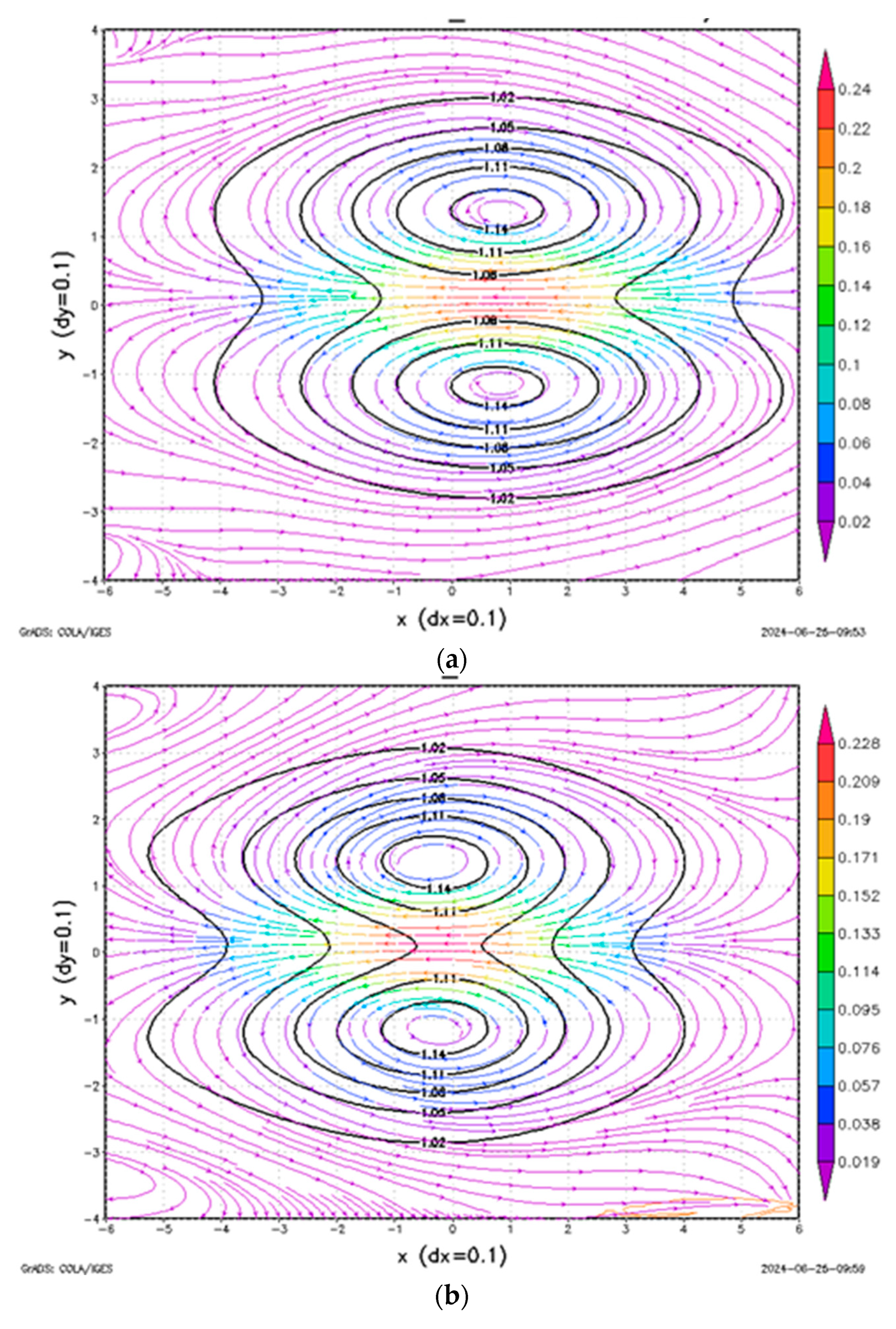
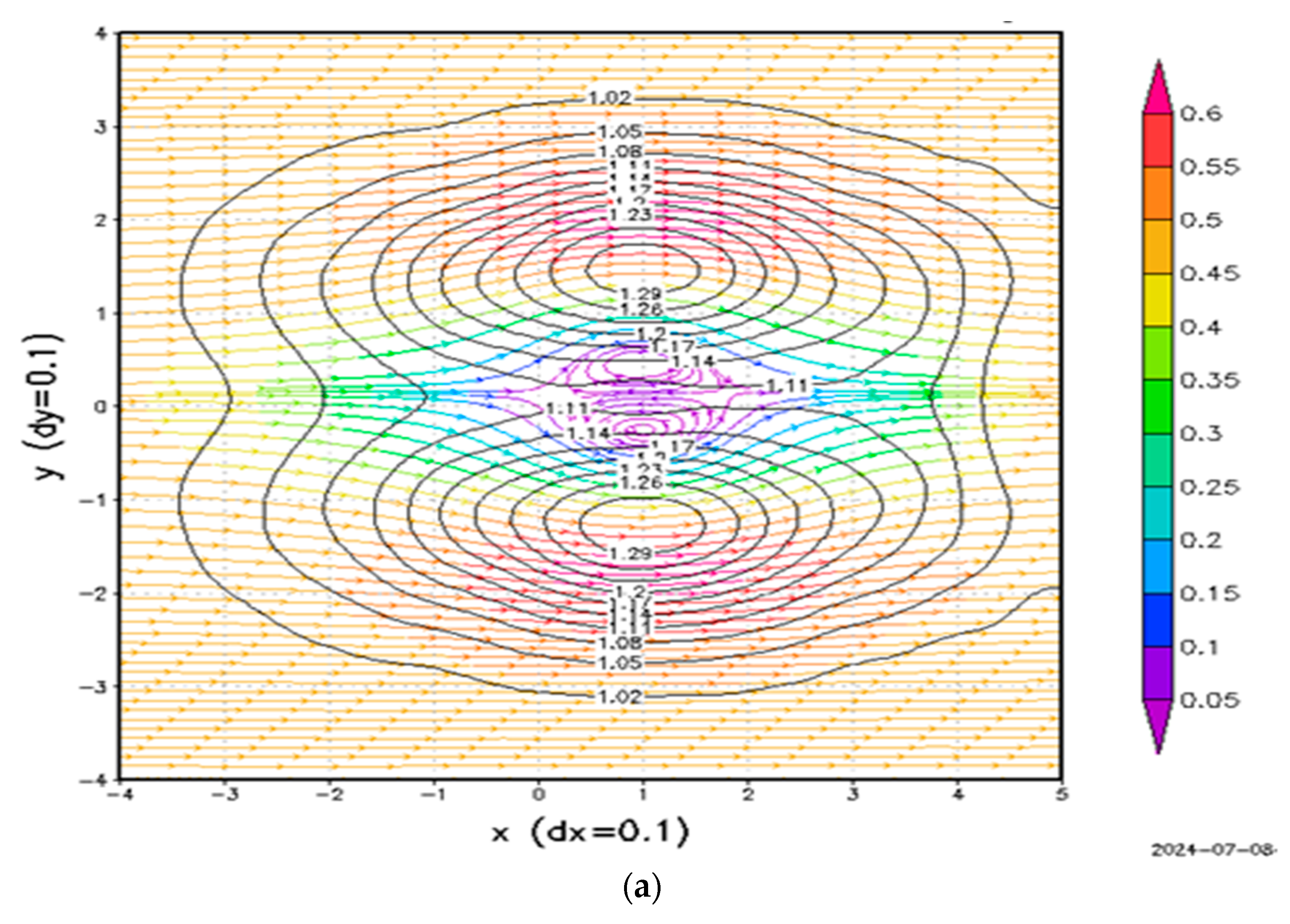
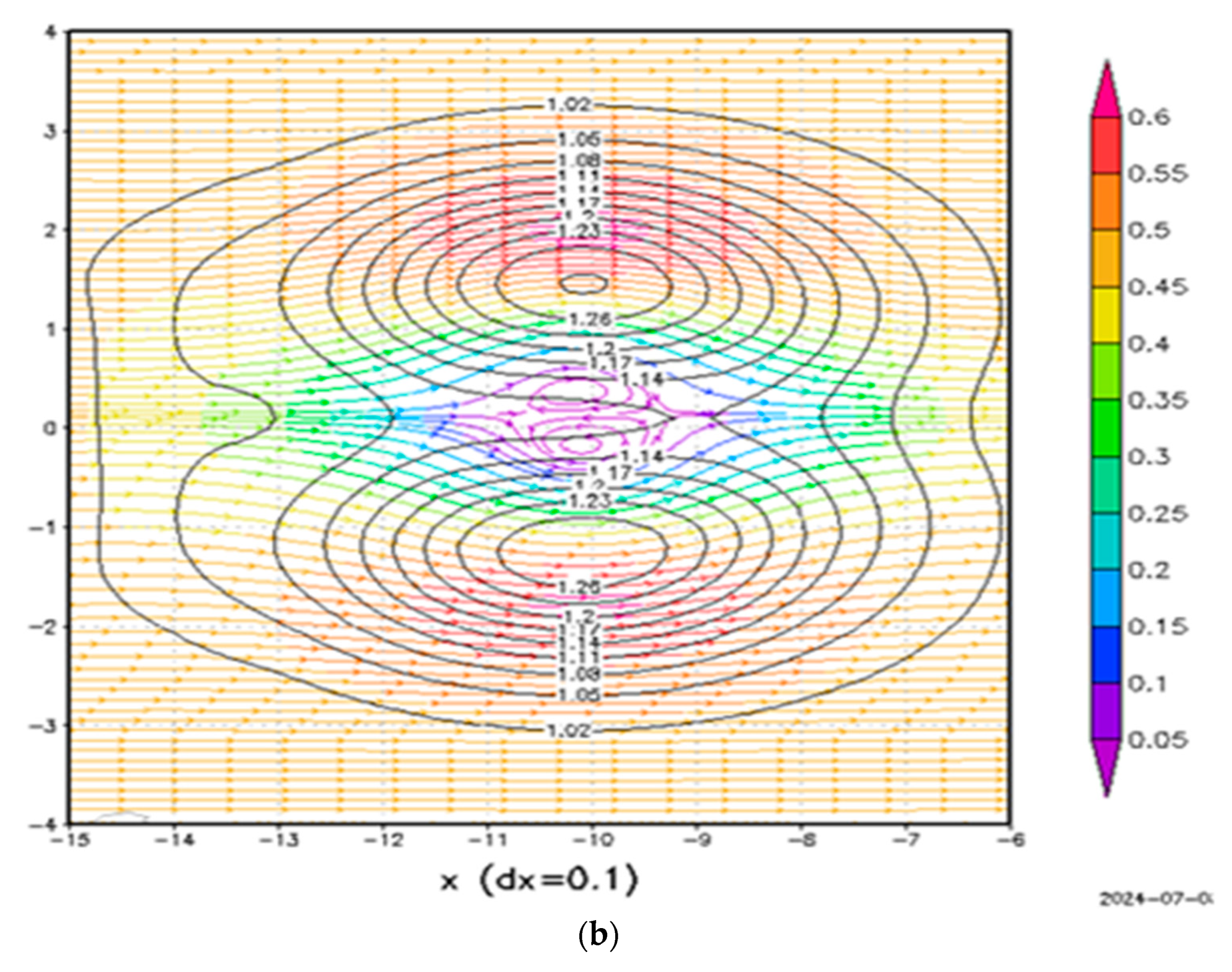
Using forward integration at t = 120 (purple in Figure 1a or black in Figure 1b) as the initial condition, the Rossby wave moves eastward as time decreases, initially at t = 120 (black), t = 90 (red), t = 60 (green), t = 30 (blue), and t = 0 (purple), as shown in Figure 1b, from backward integration. The heights and circulations after 120 time units from backward integration at t = 0 (Figure 2b) are quite comparable to its initial conditions at t = 120 in forward integration (Figure 2a). The soliton does return to its original position, but the velocity does not follow u(−t) = −u(t) as suggested by Eckhardt and Hascoët [9] or Fang et al. [10]. We conclude that the system is reversable if the change in velocity and height satisfies d ξ(−t) = −d ξ(t), which is consistent with Equations (7)–(11). The results also prove that the model without modification can be applied to both forward and backward integrations.
The total mass (Ma), energy (Eng), potential vorticity (PV), and enstrophy (He) [31] are
M a ( t ) = j = 1 J m i = 1 Im h i , j ( t ) Δ x Δ y
E n g ( t ) = 1 2 j = 1 J m i = 1 Im h i , j ( t ) u i , j 2 + v i , j 2 + g h i , j + h s i , j 2 Δ x Δ y
P V ( t ) = j = 1 J m i = 1 Im Π Δ x Δ y = j = 1 J m i = 1 Im v x u y + f / h Δ x Δ y
and
H e ( t ) = 1 2 j = 1 J m i = 1 Im h i , j q i , j 2 Δ x Δ y = 1 2 j = 1 J m i = 1 Im ς i , j + f i , j 2 h i , j Δ x Δ y
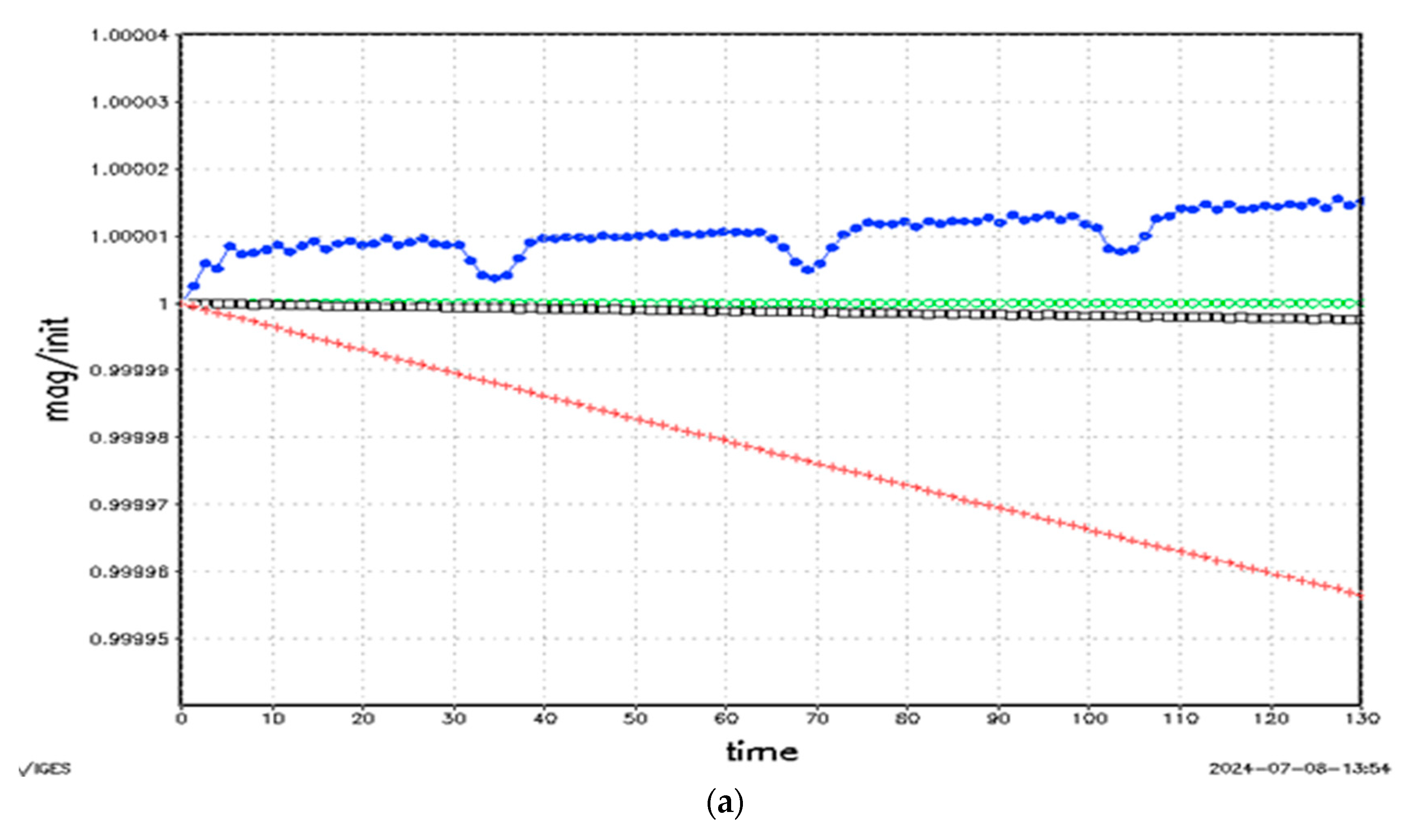
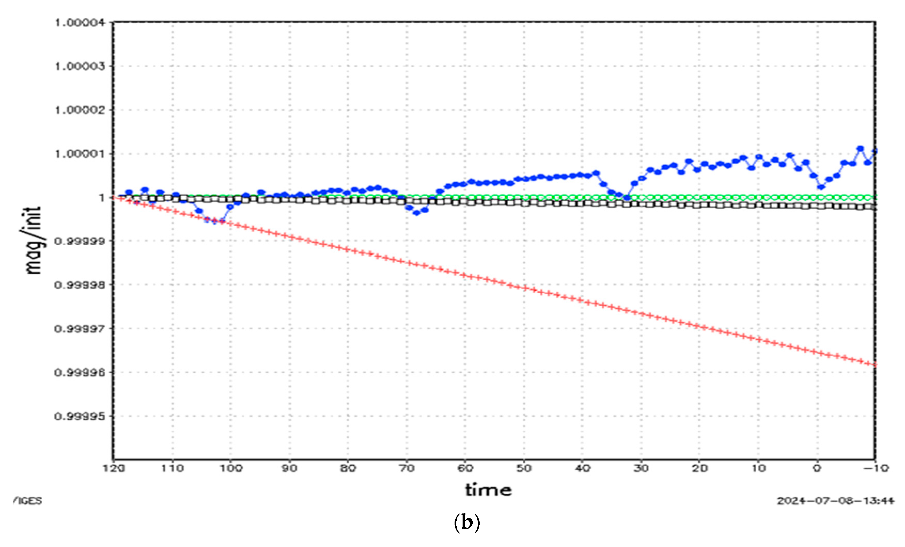
Figure 3a shows the time sequences of the ratio of the variable with respect to its initial value, Ma(t)/Ma(t = 0) by green, Eng(t)/Eng(t = 0) by red, PV(t)/PV(t = 0) by blue, and He(t)/He(t = 0) by black according to (23)–(26) from forward integration. Figure 3b shows the same, except it is from backward integration. They remain almost constant with respect to time in both integrations, although an open boundary condition is applied to the northern and southern boundaries, because the wave is trapped near the equator.

4.3. Results with B = 0.6 and CB = 0.476

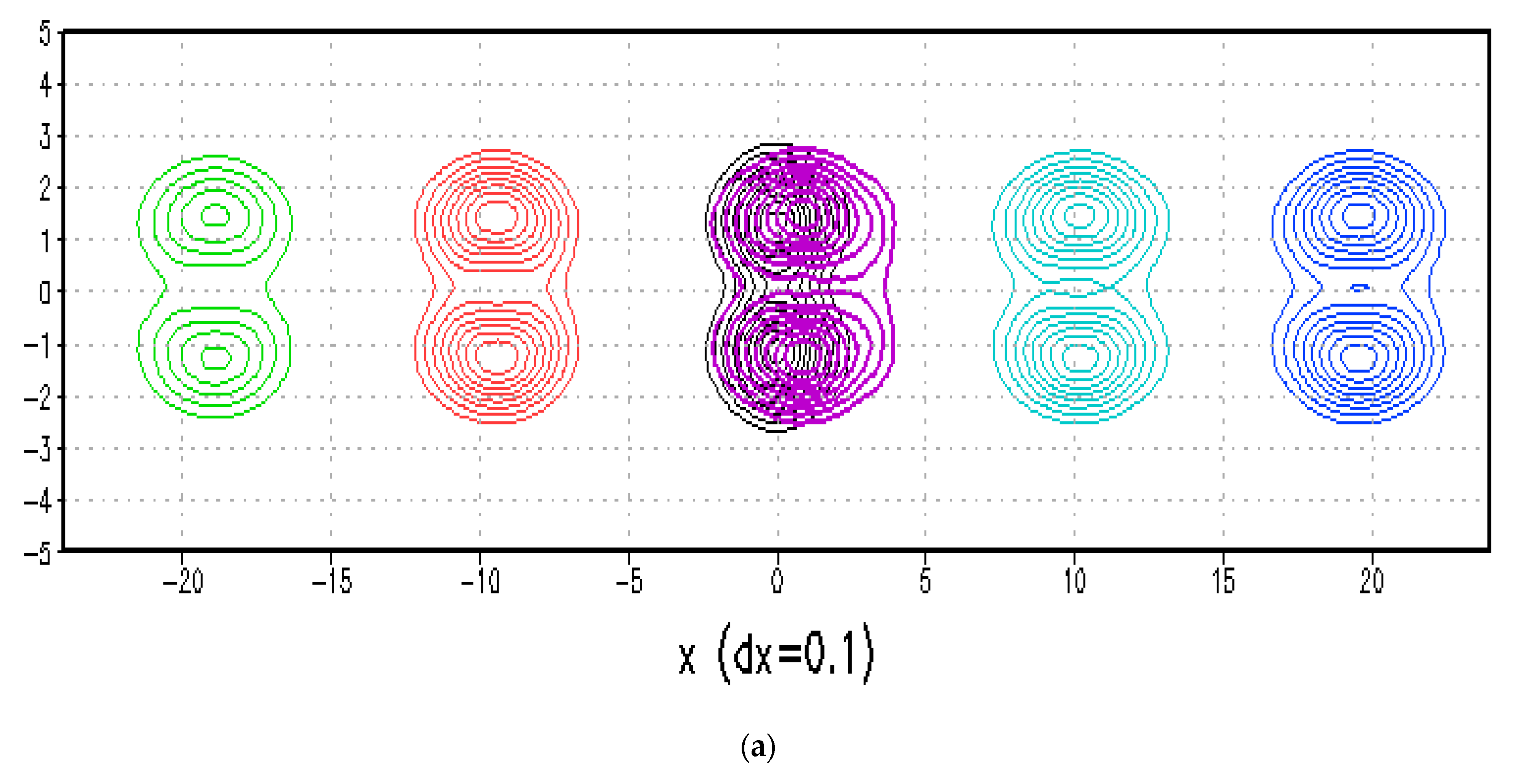
The soliton propagates westward from forward integration as shown in Figure 4a: red designates the location at t = 20, green at t = 40, blue at t = 60, light blue at t = 80, and purple at t = 100. Then, the result at t = 100 is used as an initial condition for backward integration. Red in Figure 4b shows the locations at t = 80, green at t = 60, blue at t = 40, light blue at t = 20, and purple at t = 0, as the soliton moves backward (eastward) as time decreases in backward integration. The propagating speed of the soliton is faster than in the previous case. The change in heights between t = 0 (black) and t = 100 (purple) during forward integration in Figure 4a and between t = 100 (black) and t = 0 (purple) in backward integration (Figure 4b) is larger than in the previous case with B = 0.395.
The KdV equation was derived based on asymptotic expansion of small perturbation i.e., ε = O ( ς / H ( mean   height ) ) < < 1 . According to (16) with B = 0.6, we obtain ε = 0.278 , which is consistent with the perturbation of water height shown in Figure 5a,b, but does not satisfy ε < < 1 . Hence, it needs higher-order terms to represent the KdV solution, as discussed in [29,35,36,37] and in shallow water modeling [32].
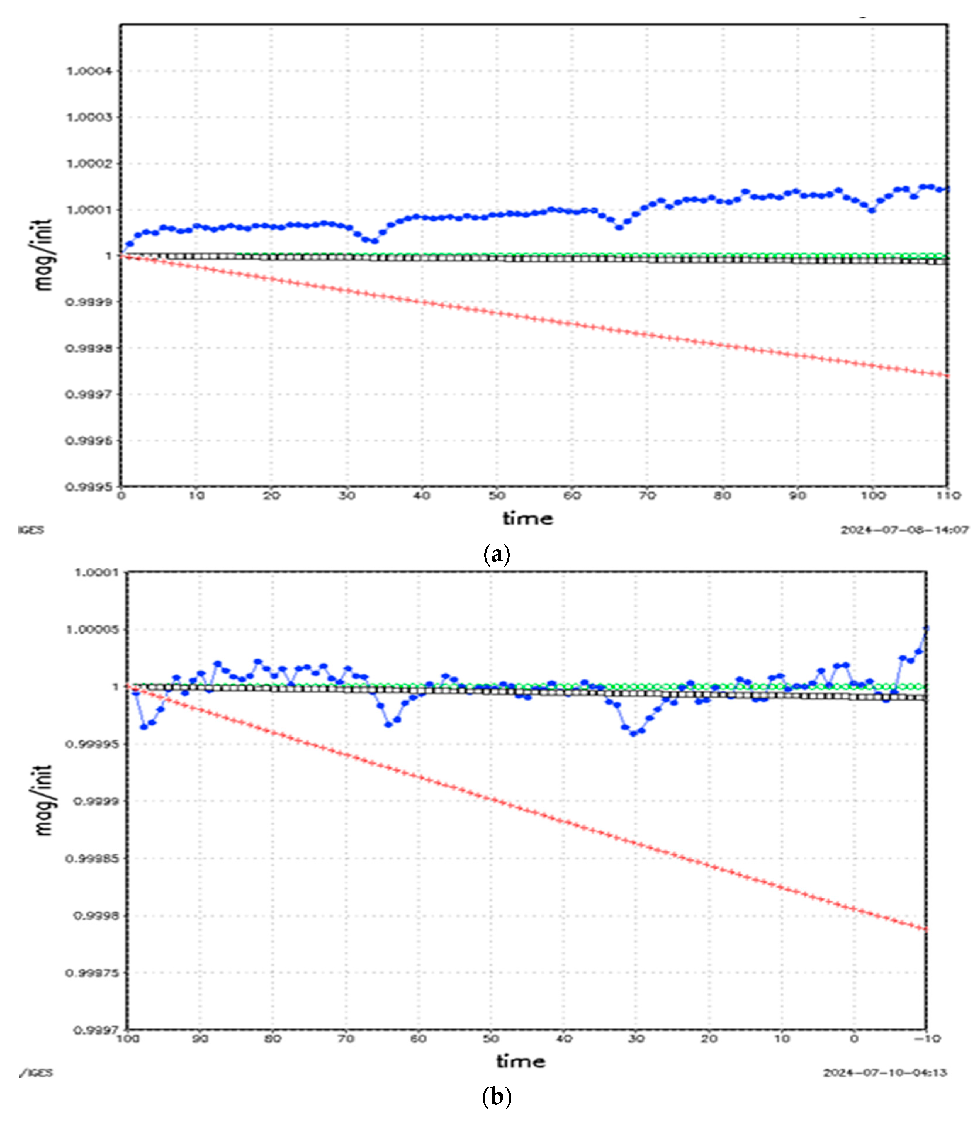
The secondary circulations with respect to the moving soliton, (u-CB, v), are like the simulations of Sun and Sun [24] and discussed in [27,28]. It is also noted that the longer the integration, the wider the spreading between long waves and short waves in advection equations [34]. Hence, distortion becomes visible after 100 time units from backward integration at t = 0 (purple) in Figure 4b. The error of phase speed can be reduced by using a more accurate advection scheme [34], the scheme combining the QUICK [38] and fourth-order schemes as shown in the simulations of Sun and Sun [24], or semi-Lagrange schemes [39,40]. The time sequences of the ratios, Ma(t)/Ma(t = 0) (green), Eng(t)/Eng(t = 0) (red), PV(t)/PV(t = 0) (blue), and He(t)/He(t = 0) (black) remain near unity in both forward and backward integrations (Figure 6a,b). The wave is trapped around the equator and the slight decrease in the total energy comes from the truncational error of the fourth-order scheme and the dispersion of phase speed among different waves.

5. Discussion

In this paper, the analytic solutions of solitary Rossby waves are used to verify the backward integrations because the shape and propagating speed of the waves do not change with time. We will present the inverse of vortices merging [31] and nonlinear shear instability [41] in Part II, in which the nonlinear terms become dominated. In the future, we will combine this inviscid nonlinear model and the subgrid turbulence diffusion models [8,23] to study the inverse of fluid dynamic systems with diffusion/viscosity. The results should be close to realistic initial values, because the subgrid turbulence diffusion model can overcome the difficulty of counter-gradient flow. It also avoids extra diffusion by changing the sign of viscosity in the traditional forward–backward integrations or the time-consuming iterative data assimilations discussed previously.

6. Summary

The shallow water model developed by Sun [1] was applied to simulate Rossby solitons in the equator. The model was integrated forward in time for 120 time units (with B = 0.395) or 100 time units (with B = 0.6), then the simulations were used as initial conditions for backward integrations. The detailed structure, secondary circulation, and propagating speed of solitons from both integrations are in good agreement with the analytic solutions of KdV. The total mass, energy, and enstrophy are also well conserved, although a slight decrease in total kinetic energy may be due to truncational errors of the fourth-order scheme and the dispersion of phase speed among different waves.
This inviscid, nonlinear model, which has neutral stability and does not need any viscosity/smoothing to control instability, can be applied to both forward and backward integrations by just changing the time step from positive to negative. Hence, not only is the procedure much simpler, but the results are also more accurate than the traditional inverse methods which can be contaminated by unwanted diffusion in forward–backward integrations, or inaccurate guesses of initial values in time-consuming iterative data assimilations.

Funding

This research received no external funding.

Institutional Review Board Statement

Not applicable.

Informed Consent Statement

Not applicable.

Data Availability Statement

The original contributions presented in the study are included in the article, further inquiries can be directed to the corresponding author.

Acknowledgments

The computing facility provided by Lin and Huang at National Central University, Taiwan, is appreciated. The author also thanks the reviewers for their comments.

Conflicts of Interest

The authors declare no conflict of interest.

References

  1. Sun, W.Y. Instability in Leapfrog and Forward-Backward Schemes: Part II: Numerical Simulation of Dam Break. J. Comput. Fluids 2011, 45, 70–76. [Google Scholar] [CrossRef]
  2. Pine, D.J.; Gollub, J.P.; Brady, J.F.; Leshansky, A.M. Chaos and threshold for irreversibility in sheared suspensions. Nature 2005, 438, 15. [Google Scholar] [CrossRef] [PubMed]
  3. Taylor, G. Low Reynolds Number Flows and Reversibility. 1967. Available online: http://web.mit.edu/hml/notes.html (accessed on 25 September 2024).
  4. Wikipedia. Taylor–Couette Flow. Available online: https://en.wikipedia.org/wiki/Taylor%E2%80%93Couette_flow (accessed on 25 September 2024).
  5. Wikipedia. Navier–Stokes Equations. Available online: https://en.wikipedia.org/wiki/Navier%E2%80%93Stokes_equations (accessed on 25 September 2024).
  6. Haltiner, G.J.; Williams, R.T. Numerical Prediction and Dynamic Meteorology, 2nd ed.; Wiley: Hoboken, NJ, USA, 1980; p. 477. [Google Scholar]
  7. Fourier, J.B.J. Theorie Analytique de la Chaleur; Didot: Paris, France, 1822; pp. 499–508. [Google Scholar]
  8. Sun, W.Y.; Sun, O.M. Backward Integration of Diffusion Equation. Aerosol Air Qual. Res. 2017, 17, 278–289. [Google Scholar] [CrossRef]
  9. Eckhardt, B.; Hascoët, E. Breaking time reversal symmetry by viscous dephasing. Phys. Rev. E 2005, 72, 037301. [Google Scholar] [CrossRef]
  10. Fang, L.; Bos, W.J.T.; Liang, S.; Bertoglio, J.-P.; Shao, L. Time reversibility of Navier-Stokes turbulence and its implication for subgrid scale models. J. Turbul. 2012, 13, 639777. [Google Scholar] [CrossRef]
  11. Kalnay, E.; Park, S.K.; Pu, Z.X.; Gao, J. Application of the Quasi-Inverse Method to Data Assimilation. Mon. Wea. Rev. 2000, 128, 864–875. [Google Scholar] [CrossRef]
  12. Sun, W.Y. Instability in leapfrog and forward-backward Schemes. Mon. Wea. Rev. 2010, 138, 1497–1501. [Google Scholar] [CrossRef]
  13. Lorenc, A.C. Analysis Methods for Numerical Weather Prediction. Q. J. R. Meteorol. Soc. 1986, 112, 1177–1194. [Google Scholar] [CrossRef]
  14. Sasaki, Y. Some basic formalisms in numerical variational analysis. Mon. Wea. Rev. 1970, 98, 875–883. [Google Scholar] [CrossRef]
  15. Le Dimet, F.; Talagrand, O. Variational algorithms for analysis and assimilation of meteorological observations: Theoretical aspects. Tellus A. 1986, 38A, 97–110. [Google Scholar] [CrossRef]
  16. Johnson, C.; Nichols, N.K.; Hoskins, B.J. Very Large Inverse Problems in Atmosphere and Ocean Modelling; Numerical Analysis Report 5/04; Department of Mathematics, University of Reading: Reading, UK, 2005. [Google Scholar] [CrossRef]
  17. Huang, S.; Xiang, J.; Du, H.; Cao, X. Inverse problems in atmospheric science and their application. J. Phys. Conf. Ser. 2005, 12, 45–57. [Google Scholar] [CrossRef]
  18. Pu, Z.-X.; Kalnay, E.; Sela, J.; Szunyogh, I. Sensitivity of forecast errors to initial conditions with a quasi-inverse linear model. Mon. Wea. Rev. 1997, 125, 2479–2503. [Google Scholar] [CrossRef]
  19. Nabi, S.; Grover, P.; Caulfield, C. Robust preconditioned one-shot methods and direct-adjoint-looping for optimizing Reynolds-averaged turbulent flows. Comput. Fluids 2022, 238, 105390. [Google Scholar] [CrossRef]
  20. O’Connor, L.; Lecoanet, D.; Anders, E.H.; Augustson, K.C.; Burns, K.J.; Vasil, G.M.; Oishi, J.S.; Brown, B.P. Iterative methods for Navier-Stokes inverse problems. Phys Rev. E. 2024, 109, 045108. [Google Scholar] [CrossRef] [PubMed]
  21. Keller, J.J. Inverse Euler equation. Z. Angew. Math. Phys. 1966, 49, 363–383. [Google Scholar] [CrossRef]
  22. Kaus, B.J.P.; Podadchikov, Y.Y. Forward and Reverse Modeling of the Three-Dimensional Viscous Rayleigh-Taylor Instability. Geo. Res. Lett. 2001, 6, 1095–1098. [Google Scholar] [CrossRef]
  23. Sun, W.Y. Diffusion modeling in a convective boundary layer. Atmos. Environ. 1989, 23, 1205–1217. [Google Scholar]
  24. Sun, W.Y.; Sun, O.M.T. Numerical Simulation of Rossby Wave in Shallow Water. Comput. Fluids 2013, 76, 116–127. [Google Scholar] [CrossRef]
  25. Boussinesq, J. Essai sur la Theorie des Eaux Courantes. Memoires Presentes par Divers Savants a L’academie des Sciences de L’institut National de France; XXIII, Imprimerie Nationale: Paris, France, 1877; pp. 1–680. [Google Scholar]
  26. Korteweg, D.J.; de Vries, G. On the change of form of long waves advancing in a rectangular canal, and on a new type of long stationary waves. London Edinburgh Dublin Philos. Mag. J. Sci. 1895, 39, 422–443. [Google Scholar] [CrossRef]
  27. Larichev, V.D.; Reznik, G.M. On two-dimensional solitary Rossby waves. Dokl. Akad. Nauk. SSSR 1976, 231, 1077–1079. [Google Scholar]
  28. Boyd, J.P. Equatorial solitary waves. Part-1: Rossby solitons. J Phys Ocean. 1980, 10, 1699–1717. [Google Scholar] [CrossRef]
  29. Boyd, J.P. Equatorial solitary waves. Part 3: Westward-traveling motions. J Phys Ocean. 1985, 15, 46–54. [Google Scholar] [CrossRef]
  30. Muccino, J.C.; Bennett, A.F. Generalized inversion of the Korteweg–de Vries equation. Dyn. Atmos. Ocean. 2002, 35, 227–263. [Google Scholar] [CrossRef]
  31. Sun, W.Y.; Oh, T.J. Vortex Merger in Shallow Water Model. Asia-Pac. J. Atmos. Sci. 2022, 58, 533–547. [Google Scholar] [CrossRef]
  32. Sun, W.Y. Challenges and Progress in Computational Geophysical Fluid Dynamics in Recent Decades. Atmosphere 2023, 14, 1324. [Google Scholar] [CrossRef]
  33. Leonard, B.P. A stable and accurate convective modelling procedure based on quadratic upstream interpolation. Comput. Methods Appl. Mech. Eng. 1979, 19, 59–98. [Google Scholar] [CrossRef]
  34. Sun, W.Y. Numerical experiments for advection equation. J. Comput. Phys. 1993, 108, 264–271. [Google Scholar] [CrossRef]
  35. Craig, W. An existence theory for water waves and the Boussinesq and Korteweg–de Vries scaling limits. Comm. Partial. Differ. Equ. 1985, 10, 787–1003. [Google Scholar] [CrossRef]
  36. Segur, H. Lecture 5: Waves in Shallow Water, Part I: The Theory; WHOI-2010-01 2009 Program of Study: Geophysical Fluid Dynamics, Nonlinear Waves; Woods Hole Oceanographic Institution: Falmouth, MA, USA, 2009; pp. 39–51. [Google Scholar]
  37. Drazin, P.G. Solitons; Lecture Note Series 85; Cambridge University Press London Mathematical Society: London, UK, 1983; ISSN 0076-0552. [Google Scholar]
  38. Versteeg, H.K.; Malalasekera, W. An Introduction to Computational Fluid Dynamics—The Finite Volume Method; Longman Scientific & Technical: New York, NY, USA, 1995; p. 257. [Google Scholar]
  39. Sun, W.Y.; Yeh, K.S. A general semi-Lagrangian advection scheme employing forward trajectories. J. R. Meteorol. Soc. 1997, 123, 2463–2476. [Google Scholar]
  40. Sun, W.Y. An efficient forward semi-Lagrangian model. Terr. Atmos. Ocean. Sci. 2024, 35, 1–6. [Google Scholar] [CrossRef]
  41. Oh, T.J. The Development and Testing of Characteristic-Based Semi-Lagrangian Two-Dimensional Shallow Water Equations Model. Ph.D. Thesis, Purdue University, West Lafayette, IN, USA, 2007. Available online: https://docs.lib.purdue.edu/dissertations/AAI3278686/ (accessed on 20 December 2020).
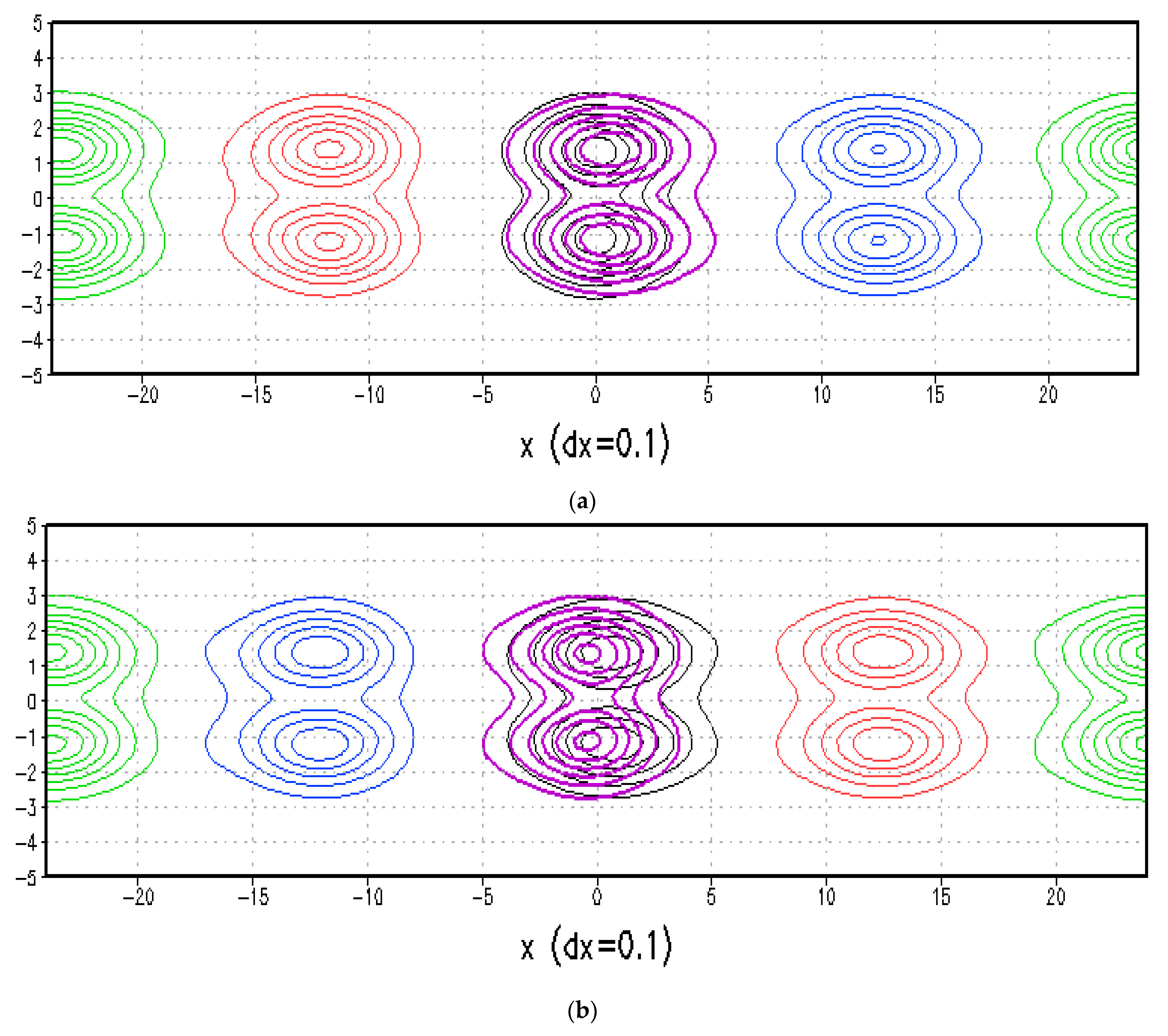
Figure 1. (a): Simulated height and location of soliton at t = 0 (black), t = 30 (red), t = 60 (green), t = 90 (blue) and t = 120 (purple). Contours are from 1.02 to 1.14 with interval of 0.025, from forward integration with B = 0.395 and CB = 0.395. Result at t = 120 is used as initial condition for backward integration. (b): Simulated height and location of soliton at t = 120 (black), t = 90 (red), t = 60 (green), t = 30 (blue) and t = 0 (purple) from backward integration. Contours are from 1.02 to 1.14 with 0.025 interval.
Atmosphere 15 01161 g001
Figure 2. (a) Simulated height (black), stream function (color), and magnitude (bar) from forward integration with B = 0.395 and CB = 0.395 at t = 120, which is used as the initial condition for backward integration. (b) Same as (a) but backward integration at t = 0 (after 120 time units from backward integration).
Atmosphere 15 01161 g002
Figure 3. (a) Time sequence of ratio of total energy (red), mass (green), potential vorticity (blue), and enstrophy (black) with respected to its initial value from t = 0 to 130 in forward integration with B = 0.395. (b) Same as (a) but backward integration from t = 120 to t = −10.
Atmosphere 15 01161 g003aAtmosphere 15 01161 g003b
Figure 4. (a) Simulated height and location at t = 0 (black), t = 20 (red), t = 40 (green), t = 60 (blue), t = 80 (light blue), and t = 100 (purple). Contours are from 1.02 to 1.29 with 0.03 interval from forward integration with B = 0.6 and CB = 0.476. (b) Simulated height and location at t = 100 (black), t = 80 (red), t = 60 (green), t = 40 (blue), t = 20 (light blue), and t = 0 (purple). Contours are from 1.02 to 1.29 with 0.03 interval from backward integration with B = 0.6 and CB = 0.476.
Atmosphere 15 01161 g004aAtmosphere 15 01161 g004b
Figure 5. (a) Simulated height (black) and stream function of relative velocity (u-CB, v) with respect to propagating speed CB and magnitude of relative velocity (bar) from forward integration at t = 100. (b) Same as (a) but backward integration at t = 20 (after 80 time units from backward integration).
Atmosphere 15 01161 g005aAtmosphere 15 01161 g005b
Figure 6. (a) Time sequence of ratios of total energy (red), mass (green), potential vorticity (blue), and enstrophy (black) to its initial values for B = 0.6 and from t = 0 to 110 in forward integration. (b) Same as (a) but backward integration from t = 100 to −10.
Atmosphere 15 01161 g006
Disclaimer/Publisher’s Note: The statements, opinions and data contained in all publications are solely those of the individual author(s) and contributor(s) and not of MDPI and/or the editor(s). MDPI and/or the editor(s) disclaim responsibility for any injury to people or property resulting from any ideas, methods, instructions or products referred to in the content.