Signs of Slowing Recovery of Antarctic Ozone Hole in Recent Late Winter–Early Spring Seasons (2020–2023)

Abstract

Every year since the early 1980s, the ozone hole has appeared in late winter/spring over Antarctica. The ozone hole is expected to disappear due to the observed decrease in the concentration of ozone-depleting substances in the stratosphere, which is enforced by the 1987 Montreal Protocol and its subsequent amendments. However, large ozone holes have appeared four years in a row (2020–2023), which may be a signal that Antarctic ozone repair has stopped. Statistical analyses of ozone hole metrics (hole area, minimum total column ozone, ozone mass deficit, and ozone mass deficit per unit area of the hole) are presented to determine how adding the data from these years changes the ozone recovery pattern. Statistically significant trends in the hole metrics were revealed for the short period (2000–2019) but not for the longer period (2000–2023). The modeled time series of metrics from multiple regressions with standard chemical and dynamic explanatory variables indicate that the recovery has slowed since around 2010. Moreover, a sequence of extreme events (wildfires in Australia in the summer of 2019/2020 and the eruption of the Hunga Tonga volcano in January 2022) may have caused additional ozone losses in Antarctica that masked the repair of polar ozone for a while.

1. Introduction

The depletion of the stratospheric ozone layer in extratropical regions due to man-made chlorine and bromine species has been a widely discussed issue since the early 1980s, which was triggered by the discovery of the so-called Antarctic ozone hole [1,2,3]. Every year in austral winter, a strong vortex is formed, which isolates Antarctica from warmer Southern Hemisphere (SH) mid-latitudes and results in extreme cooling in this region. During the Australian spring, a specific combination of low temperature (below 200 K), sunlight, polar stratospheric clouds (PSCs), and high concentrations of ozone-depleting substances (ODSs) in the stratosphere causes rapid catalytic destruction of lower stratospheric ozone [4].

The threat of increased harmful UV radiation at the surface prompted the signing of the Montreal Protocol (MP) in 1987 to control the production of long-lived halocarbons that decompose in the stratosphere, destroying the ozone layer. Under the MP and its subsequent amendments, there has been a significant decline in the production and use of ODSs [5]. Modeling studies show that declines in stratospheric ODS concentrations began in the mid-latitudes and Antarctica in the mid-1990s and early 2000s, respectively [6]. Since then, the beginning of ozone layer repair has been expected, including the disappearance of the ozone hole (i.e., hole recovery) [7,8].

Various metrics have been proposed by the National Aeronautics and Space Administration (NASA) Ozone Watch to monitor the state of the Antarctic ozone hole, including the polar cup (63°–90° S) total column ozone (TCO₃), the area of the hole, the minimum TCO₃ south of 40° S, and the ozone mass deficit [9]. The mass of the ozone deficit per unit area of the hole was also examined [10].

Numerous papers have indicated the first signs of the hole recovery related to lowering the concentration of ODSs in the stratosphere since the early 2000s [10,11,12,13,14,15]. Typically, changes in hole metrics have been associated with changes in equivalent effective stratospheric chlorine (EESC), which parameterizes ODS concentrations in the stratosphere weighted according to the ozone-depleting power of ODS species. EESC values are estimated from observed surface ODS emissions and modeled transport from the source regions in NH mid-latitudes to the lower stratosphere [16]. Since many ODSs have long residence times in the stratosphere, even the current full reduction in their production will result in the persistence of the hole for many decades to come. However, it cannot be ruled out that new substances with the potential to deplete ozone in the stratosphere that have not yet been banned by international legislation protecting the ozone layer will be used by industry, delaying the regeneration of the ozone hole.

Montzka et al. [17] proposed the ozone-depleting gas index (ODGI) to show the current state of pollution of the Antarctic atmosphere by ODSs. The ODGI represents the current change in EESC from its maximum value in 2001, expressed as a percentage of the change in EESC between 1980 (when the ozone hole was first observed) and 2001. The ODGI value in 2023 was 72.8%. This means that by this year almost 27.2% of the EESC had been removed from the Antarctic atmosphere since the EESC maximum in 2001. The current rate of change of the ODGI is about −1.3% per year, which means that EESC will return to its 1980 value around 2077 [17].

In 2019, the hole was unusually small due to the stratospheric warming that occurred in mid-September [18]. Thus, trend analyses for periods ending in 2019 provided evidence of an even more rapid recovery of the ozone hole than would result from the reduction in the stratospheric ODS concentration between 2000 and 2019 [10]. Averaging the daily values of the ozone mass deficit and the ozone mass deficit per unit area of the hole from September 1 to 30 and from September 15 to October 15, the rates of recovery by 2019 were about twice as fast as the corresponding rate of recovery of EESC. This resulted in a year of metric recovery at least 20–30 years earlier than the year in which EESC would return to its 1980 value.

In 2020, large wildfires were observed in Australia that might have influenced the SH stratospheric ozone [19,20]. Moreover, the Hunga Tonga volcano eruption in January 2022, which put a large amount of water vapor into the stratosphere [21], could also affect the SH polar vortex and the ozone destruction rate in the lower stratosphere during the ozone hole period. This year, on September 21, the area of the ozone hole reached 26 million km², one of the largest holes ever observed on this day of the year, although the largest hole in history occurred in 2000 (29.9 million km² on 9 September).

In this paper, we examine the long-term (1980–2023) changes in the Antarctic hole metrics, with a particular focus on the impact of metric fluctuations over the past four years (2020–2023) on the pattern of ozone recovery. The question is whether statistical analyses of the extended time series of the metrics from 1979 to 2023 will further support the recovery of ozone in Antarctica. This paper uses standard statistical methods to detect the slowdown in the ozone recovery based on time-series analyses of various ozone hole metrics.

This paper is organized as follows: Section 2.1 describes the data sets used, metrics of the hole, and potential variables explaining changes in the metrics. Section 2.2 presents the statistical models used to reveal the continuation (or slowdown) of the SH polar ozone recovery due to the inclusion of new data from the past four years. Long-term changes in the metrics and the effects of proxies are shown in Section 3. A discussion and conclusions are presented in Section 4.

2. Materials and Methods

2.1. Data

The long-term variability of Antarctic ozone is analyzed using the following metrics of the TCO₃ distribution in the SH polar region: polar cup TCO₃ (averaged TCO₃ over the 63°–90° S region), ozone hole area (the area of the region with TCO₃ < 220 DU), minimum TCO₃ within the hole, mass of the ozone deficit (difference between actual TCO₃ within the hole and the hole threshold of 220 DU integrated over the entire hole area), and mass of the O₃ deficit per unit area (mass of the TCO₃ deficit within the entire hole divided by its area).

Table 1. Metrics of the SH polar total column ozone.

Metrics	Unit	Short Name	Period
Mean TCO3 in polar cup from MERRA-2 reanalysis	DU	Polar_Cup_MERRA	1980–2023
Mean TCO3 in polar cup from satellite data	DU	Polar_Cup_SAT	1979–2023
Ozone hole area	km2	Hole_Area	1979–2023
TCO3 minimum in SH	DU	O3_Min	1979–2023
Mass of TCO3 deficit	ton	O3_Deficit	1980–2023
Mass of ozone deficit per 1 km2 area of hole	ton km−2	O3_Deficit_Dens	1980–2023

shows the details of the considered TCO₃ data base. For the first considered metric, the data are taken from the Modern-Era Retrospective analysis for Research and Applications, Version 2 (MERRA-2) simulations of the global TCO₃ field. The data set used is M2T1NXSLV_5_12_4_TO3 [22]. For other variables, the data sources are satellite TCO₃ observations by the Total Ozone Mapping Spectrophotometer (TOMS), Ozone Monitoring Instrument (OMI), and Ozone Mapping and Profiler Suite (OMPS) instrument. More details of these data can be found on the NASA Ozone Watch (NO₃W) website [9]. There were no satellite observations in 1993 and 1995. Therefore, a comparison between the statistical analyses of Polar_Cup_MERRA and Polar_Cup_SAT will allow a discussion of whether the lack of observations affected the pattern of long-term changes in the latter metric.

NO₃W uses the Hole_Area, O₃_min, and O₃_Deficit metrics to monitor the state of the ozone hole on a daily basis [9]. The mean values of Hole_area and O₃_min are calculated by averaging the size of the hole and the TCO₃ minima for the periods of 7 September–13 October and 21 September–16 October, respectively. For O₃_Deficit, the averaging period is 21 September–13 October. For Polar_Cup_MERRA and Polar_Cup_SAT, the averaging period is 13 September–5 October. These averaging periods are used by NO₃W to present annual variations (1979–2023) in the SH polar ozone metrics. The last metric in Table 1, O₃_Deficit_Dens, i.e., the ratio between the ozone mass deficit and the hole area, was proposed to monitor changes in the rate of ozone destruction within the hole [10]. The annual value of the O₃_Deficit_Dens metric is shown as the average value taken from the daily O₃_Deficit_Dens values for the period from 21 September to 13 October, the same period that NO₃W selected for O₃_Deficit.

In addition, the daily TCO₃ values from the satellite overpasses of Halley Bay station (75.54° S, 27.41° W) for the period 1979–2023 are considered to obtain the corresponding late winter/early spring (7 September–13 October) TCO₃ means. The SBUV Merged Ozone Data Set for the period 1979–2022 [23] and very recent (for 2023) TCO₃ observations by the OMPS [24] are combined for this station.

Table 2. Variables associated with the metrics shown in Table 1.

Variables	Unit	Short Name	Data Source
PSC Type 1 (NAT) Volume	km3	Vol_PSC_NAT	“Volume PSC NAT” subset from https://ozonewatch.gsfc.nasa.gov/meteorology/temp_2023_MERRA2_SH.html
PSC Type 2 (ICE) Volume	km3	Vol_PSC_ICE	“Volume ICE” subset from https://ozonewatch.gsfc.nasa.gov/meteorology/temp_2023_MERRA2_SH.html
Minimum Air Temperature at 50/100 hPa	K	TMIN,50hPa and TMIN,100hPa	“Minimum temperature” subset from https://ozonewatch.gsfc.nasa.gov/meteorology/temp_2023_MERRA2_SH.html

shows variables that are important for the discussion of the appearance of the ozone hole in Antarctica, i.e., the stratospheric temperature and PSC volume. These characteristics will be used in Section 3 to discuss sources of variability in the metrics in the period 1980–2023.

Variables that can be associated with ozone variability in Antarctica, i.e., the so-called explanatory variables, are used as inputs in the stepwise regression to model oscillations in the SH polar ozone metrics. The explanatory variables considered here are shown in

Table 3. Explanatory variables used in the stepwise regression of the SH polar ozone metrics.

Variables	Unit	Short Name	Data Source
Equivalent effective stratospheric chlorine	ppt	EESC	https://gml.noaa.gov/odgi/
10.7 cm solar flux	Wm−2	SF10.7cm	https://climexp.knmi.nl/data/isolarradioflux.dat
Antarctic Oscillation Index	−	AAO	https://www.cpc.ncep.noaa.gov/products/precip/CWlink/daily_ao_index/aao/aao.shtml
Multivariate ENSO Index	−	MEI	https://www.psl.noaa.gov/enso/mei
Quasi-Biennial Oscillations Index at 30 hPa and 50 hPa	ms−1	QBO30hPa and QBO50hPa	https://www.cpc.ncep.noaa.gov/data/indices/qbo.u30.index https://www.cpc.ncep.noaa.gov/data/indices/qbo.u50.index
Zonal wind at 70 hPa level along 60° S	ms−1	U_60S	https://acd-ext.gsfc.nasa.gov/Data_services/met/ann_data.html
Stratospheric Aerosol Optical Depth at 750 nm for 80° S	−	AOD750nm	www.columbia.edu/~mhs119/StratAer/ and after 1984 https://fmi.b2share.csc.fi/records/8bfa485de30840eba42d1d407f4ce19c
45-Day Mean 45°–75° S Heat Flux at 70 hPa level	Kms−1	HF70hPa	https://ozonewatch.gsfc.nasa.gov/meteorology/flux_2023_MERRA2_SH.html
SH vortex area at 460 K level	km2	Vor_Area	https://ozonewatch.gsfc.nasa.gov/meteorology/pv_2023_MERRA2_SH.html
Dipole Mode Index	K	DMI	https://climexp.knmi.nl/data/idmi_ersst.dat

“−” indicates dimensionless variable. All web addresses were accessed on 1 December 2023.

.

2.2. Statistical Models

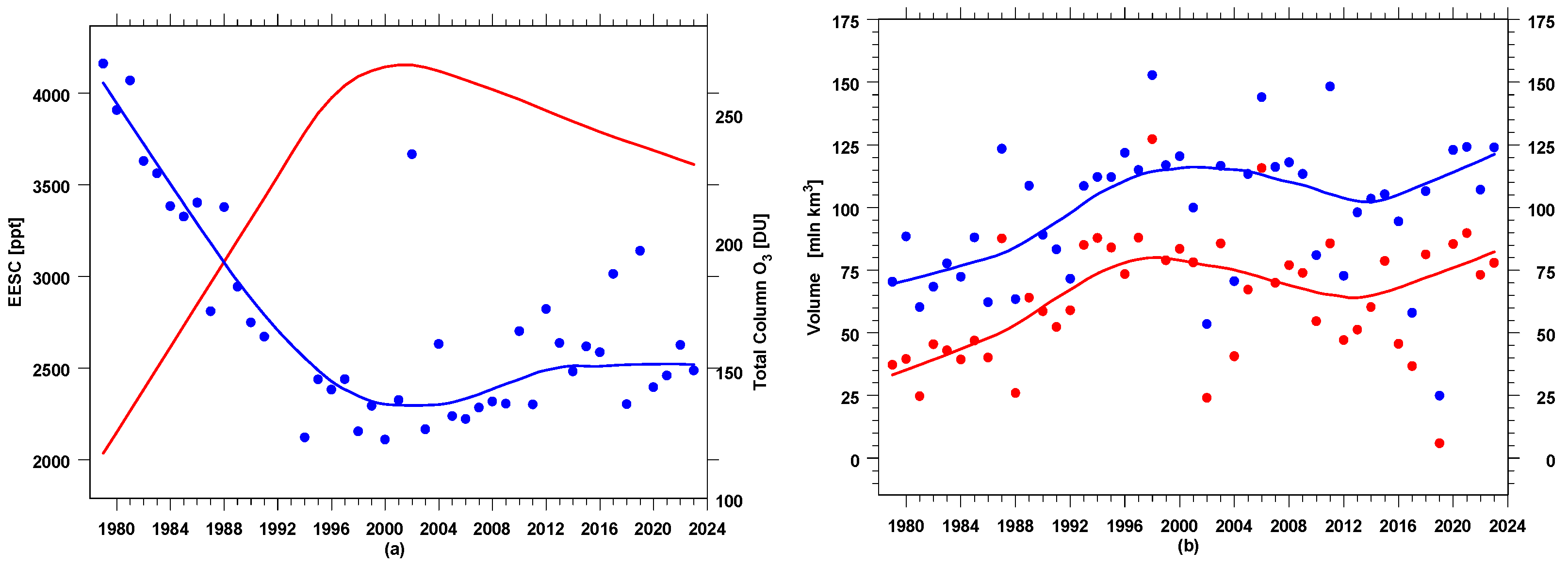
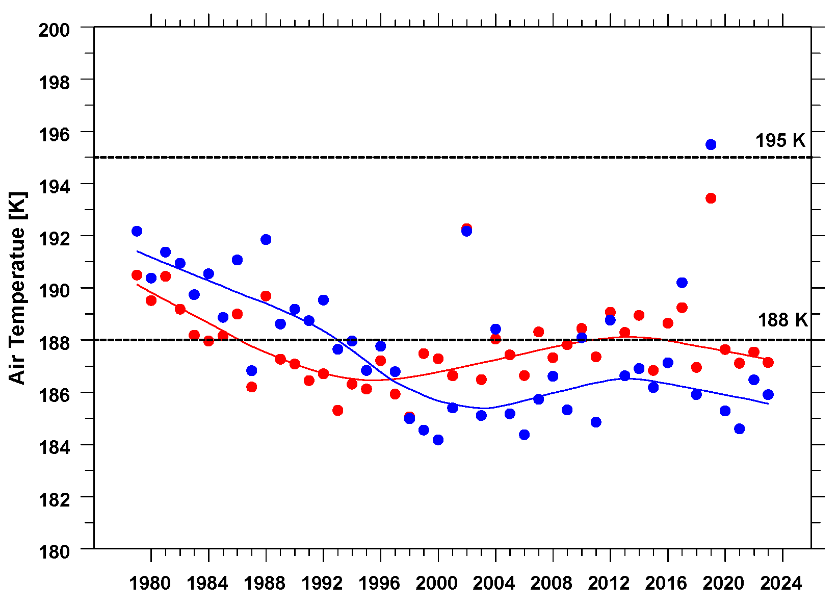
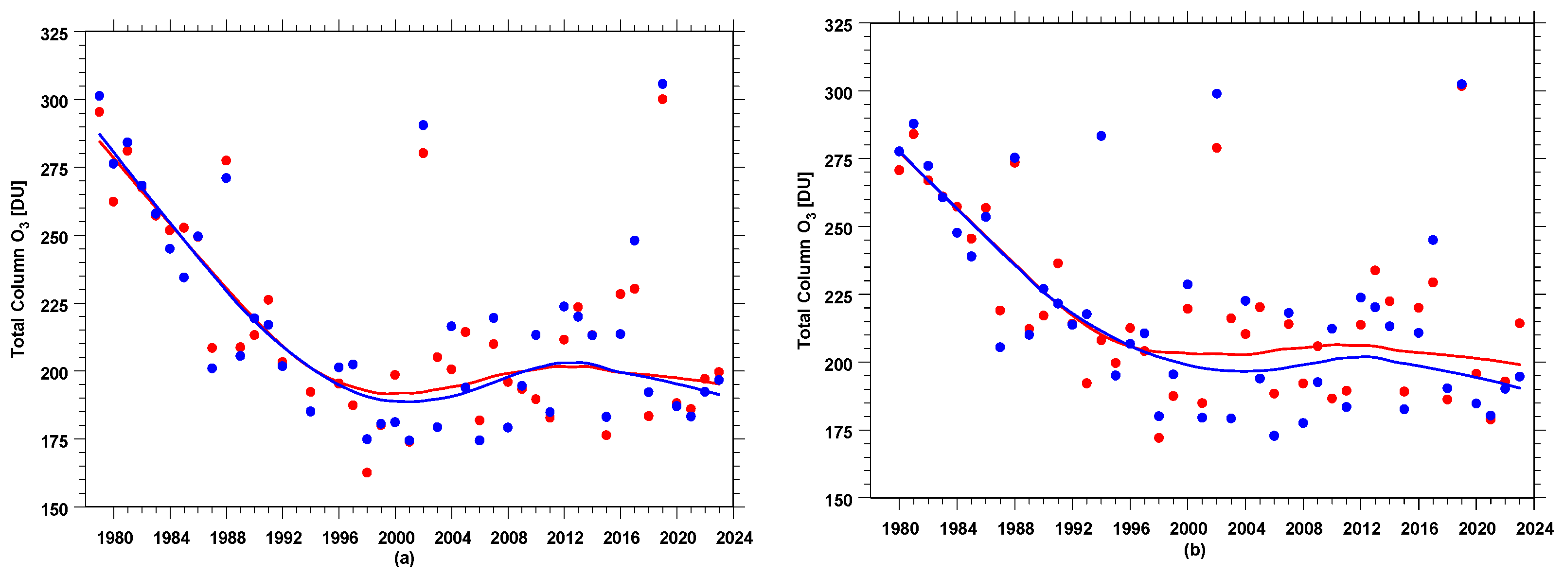
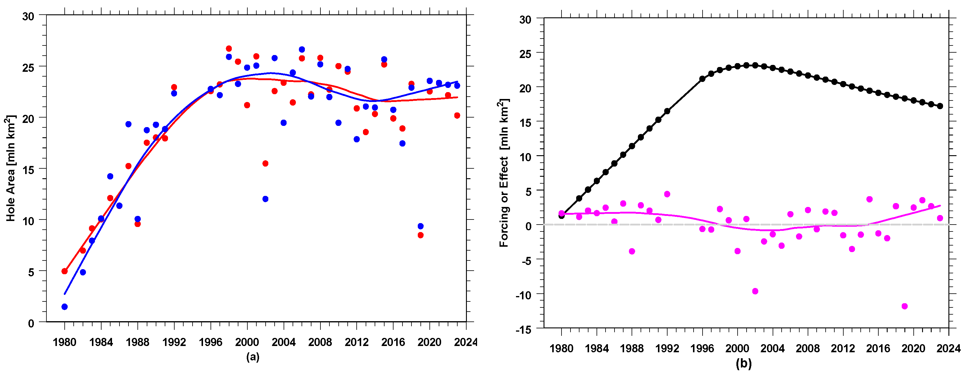
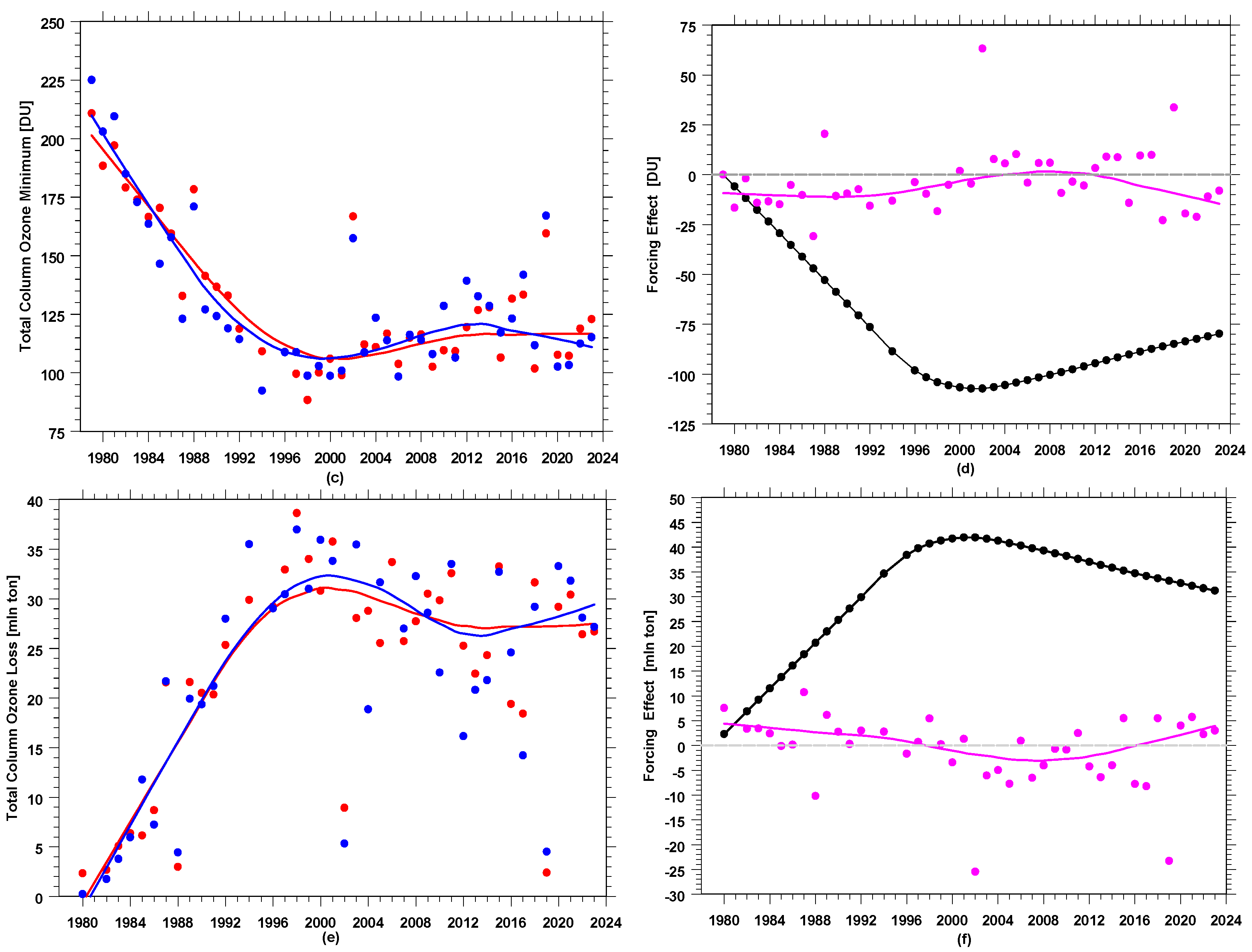
A standard least-squares linear regression is used to calculate trends in the SH polar ozone metrics for the periods 2000–2019 and 2000–2023. The trend comparison allows a discussion of the changes in the rate of ozone recovery in Antarctica that occur when data from the last four years (2020–2023) are added.

A prerequisite for using any variable in a regression is its independence from the variable being regressed. Ozone absorbs solar UV radiation, which warms the air and contributes to the formation of the stratosphere. The temperature effect due to the stratospheric ozone influences PSCs, as they appear when the temperature drops below 195 K (PSC NAT) and 188 K (PSC ICE). Therefore, the variables shown in Table 2 (Vol_PSC_NAT, Vol_PSC_ICE, T_MIN,50hPa, and T_MIN,100hPa) are not considered as potential independent explanatory variables; however, their long-term variability is important for understanding ozone trends and will be discussed further in the text (Section 3 and Section 4).

A stepwise regression is used to find the optimal set of explanatory variables containing only variables that significantly affect the response variable. The minimum value of the Akaike Information Criterion (AIC) is used when searching for this optimal set of explanatory variables. The EESC proxy is used to describe the chemical forcing on the metrics due to ODS changes. Other variables are used to account for the dynamical effects due to the teleconnection pattern (AAO, MEI, QBO, and DMI), proxies related to the strength of the polar vortex (HF_70hPa, U_60S, and Vor_Area), external solar forcing (SF_10.7cm), and aerosol effects (AOD_750nm). The regression has the following form:

$$Metrics={\alpha }_0+ {{\displaystyle \sum }}_{i=1}^N{a}_i{X}_i+Noise$$

(1)

where statistically significant explanatory variables, $X_i$, are taken from the final output of the stepwise regression and N is the number of such variables. These variables are selected from the full set of variables (Table 3): EESC, SF_10.7cm, AAO, MEI, QBO_30hPa, QBO_50hPa, DMI, HF_70hPa, U_60S, Vor_Area, and AOD_750nm.

Further in the text, $a_{1}EESC$ and ${{\displaystyle \sum }}_{i=2}^N{a}_i{X}_i$ will be marked as EESC and combined non-EESC forcing, respectively. For any metric, if stratospheric aerosols do not appear in the list of statistically significant explanatory variables, the former and latter forcing variables represent the chemical and overall dynamical forcing, respectively.

Statistical calculations (trend coefficient, stepwise regression, and data smoothing) are based on S-PLUS software [25]. A lowess filter is used to smooth the time series [26].

3. Results

EESC has been declining almost linearly since the 2000–2001 peak (Figure 1a), and it can be expected that a corresponding increase in TCO₃ should follow the EESC pattern. Satellite observations over the Antarctic Halley Bay station show that TCO₃ has stabilized since the early 2010s (Figure 1a). Before the appearance of the ozone hole, in late winter and early spring, PSC NAT and PSC ICE were always present in the Antarctic stratosphere. A strong decline in ozone began around 1980, when EESC exceeded a threshold of about 2000 ppt. This decrease caused a cooling of the stratosphere, which affected the appearance of PSCs (Figure 1b), resulting in a further decrease in ozone. PSC volume was positively correlated with EESC until the early 2010s. Since then, an inverse correlation has emerged. At the end of the analyzed period, the cloud volume of both PSC NAT and PSC ICE was close to the maximum value reached around 2000.

Figure 2 shows additional cooling of the stratosphere at 100 hPa and 50 hPa over the last four years (2020–2023), allowing more PSC ICE to occur between the 100 hPa and 50 hPa levels. Conditions for PSC NAT existed throughout the entire analyzed period.

Figure 3 shows time series of the SH polar cup ozone based on the TCO₃ observations (TOMS + OMI + OMPS, Figure 3a) and MERRA-2 simulations (Figure 3b). In both cases, the second overturning of the long-term TCO₃ pattern occurred around 2010. The TCO₃ values at the end of the series (2023) were only slightly higher than those near the first overturning around 2000. Similar long-term patterns were found using original MERRA-2 and satellite data (blue curves in Figure 3a,b).

The hole area in 1998 was 25.8 million km², exceeding 23 million km² for the first time (see the reference line of 23 million km² in Figure 4a). This also happened in the next three consecutive years (1999–2001), corresponding to the period of the EESC maximum in Antarctica. Another such case was found in the period 2020–2023.

Hole areas over 23 million km² were found in 13 of 26 years (1998–2023). This means that the probability of a hole >23 million km² can be estimated at 0.5, and according to Bernoulli’s test, the probability of 4 years in a row with holes >23 million km² is (0.5)⁴ = 0.0625, i.e., close to the 0.05 threshold commonly used in statistical significance calculations. Therefore, the appearance of this sequence by chance is unlikely, indicating unusual behavior of the ozone hole over the past four years.

Figure 4 also confirms the emergence of the second overturning for other ozone hole metrics. The solid and dashed smoothed curves (in blue) represent long-term variations in the analyzed series for the periods 1980–2023 and 1980–2019, respectively. The curves drawn for the shorter period have a parabolic shape similar to the EESC pattern, i.e., without the second extreme. Adding data from the additional four-year period (2020–2023) results in a second overturning. Solid and dashed lines (in red) are obtained from a standard linear regression using the least-squares method for the long (2000–2023) and short (2000–2019) data, respectively. The slopes of the lines for the shorter period are steeper than those obtained for the longer period, confirming the recent slowdown in ozone recovery in Antarctica.

The slope values, together with corresponding standard errors, are given in

Table 4. Linear trends and corresponding standard deviations from a standard least-squares regression applied to SH polar ozone metrics for the periods 2000–2019 and 2000–2023. Short names of the metrics are taken from Table 1.

Metrics (Short Names)	Linear Trends		Trend Coefficient Dimension
	2000–2019	2000–2023
Polar_Cup_SAT	2.00 ± 1.37 *	0.47 ± 1.02	DU/yr
Hole_Area	–0.26 ± 0.17 *	–0.08 ± 0.13	million km2/yr
O3_Min	1.40 ± 0.67 **	0.36 ± 0.54	DU/yr
O3_Deficit	–0.61 ± 0.37 *	–0.20 ± 0.28	million ton/yr
O3_Deficit_Den	–0.20 ± 0.10 **	–0.08 ± 0.08 *	ton km−2/10 yr

* and ** denote statistically significant results at the 1 σ and 2 σ levels, i.e., corresponding to the significance levels of about 68% and 95%, respectively, assuming a normal distribution.

. For two metrics (O₃_Min and O₃_Deficit_Dens), statistically significant recovery (at 2 σ) was calculated in the 2000–2019 period. For three metrics (Polar_Cup_SAT, Hole Area, and O₃_Deficit), recovery was found at the 1 σ level. In the longer period, ozone recovery was revealed for only one metric, O₃_Deficit_Dens, at the 1 σ level.

Figure 5 shows the time series of the ozone metrics from satellite observations (TOMS + OMI + OMPS) and model (1) (left-hand side). The figures on the right illustrate the part of the modeled time series due to EESC changes and the total effects of other explanatory variables (linear combination of statistically significant dynamical proxies and/or the aerosol proxy).

Table 5. Formulas for regression model (1) of SH polar ozone metrics and the corresponding determination coefficients (R²). Short names of the metrics and explanatory variables are taken from Table 1 and Table 3, respectively. $EES{C}_{\Delta }$ means the difference between EESC value and its value in 1979.

Metrics (Short Names)	Regression Model	R2
Polar_Cup_SAT	$487.6-0.0531·EES{C}_{\Delta }+7.593·AAO-3.785·MEI-$  $4.770·U\_60S-1.317·Vor\_Area-2.995·H{F}_{70hPA}$	0.92
Hole_Area	$-0.7952+0.0109·EES{C}_{\Delta }+46.45·AO{D}_{750nm}+$  $0.3037·U\_60S+0.6121·H{F}_{70hPA}$	0.89
O3_Min	$412.1-0.0506·EES{C}_{\Delta }+0.0701·S{F}_{10.7\mathrm{cm}}+6.035·AAO-$  $3.476·MEI-3.880· U\_60S-1.611·Vor\_Area$	0.91
O3_Deficit	$-67.15+0.0198·EES{C}_{\Delta }-2.242·AAO+1.385·MEI+$  $1.256· U\_60S+0.490·Vor\_Area+0.5822·H{F}_{70hPA}$	0.88
O3_Deficit_Dens	$-2.579-0.6744·{10}^{-3}·EES{C}_{\Delta }-0.0835·{10}^{-2}·S{F}_{10.7cm}-$  $0.092·AAO+0.0442·MEI+0.048·U\_60S+0.0208·Vor\_Area$	0.89

shows the corresponding formulas for the linear combination of explanatory variables and the coefficient of determination, showing the quality of the fit of model (1) to the observed data. The determination coefficients are high for all metrics, i.e., about 0.9, which gives a multiple correlation coefficient of about 0.95. This high value of the coefficient of determination is due to the fact that the modeled metric pattern reproduces the large changes in metric values over the period 1980–2000 forced by the increase in ODS concentration in the lower Antarctic stratosphere.

The smoothed modeled time series, shown in Figure 5, do not contain a second overturning as observed in the original time series in the early 2010s. Instead, a stabilization in the modeled metrics has been found since then. This means that the superposition of non-EESC effects has offset the effect of the main driver, i.e., changes in the ODS concentration in the lower stratosphere, resulting in a continuous shrinking of the Antarctic ozone hole since the beginning of the 21st century and the recovery of ozone in the polar cup. The second overturning in the long-term pattern of the metrics appears to be due to other factors not included in the list of possible drivers (Table 3) of ozone changes in Antarctica. However, the model is able to reproduce the second overturning in the SH polar cup TCO₃ from the satellite data (Figure 3a). This will be further discussed in Section 4.

4. Discussion and Conclusions

Large ozone holes over Antarctica with average (7 September–13 October) hole areas >23 million km² appeared four years in a row (2020–2023). The first was observed in 1998, and a sequence of four years in a row with large holes was found between 1998 and 2001. The sequence reappeared after almost twenty years. The appearance of this sequence by chance is unlikely, with a probability of about 0.05. Adding four years of data to the 1980–2019 series completely changes the pattern of long-term changes in the analyzed SH polar ozone metrics. Previously (before 2020), it was parabolic with a maximum coinciding with the extreme ODS concentration in the stratosphere, but a second maximum was identified in the early 2010s (Figure 4) in the longer (1980–2023) time series. The comparison of the linear trend values of the metrics for the shorter (2000–2019) and longer (2000–2023) periods showed that the first signs of recovery (i.e., statistically significant trends) appeared in the shorter period but disappeared when the longer time series of the metrics were analyzed.

The time series of the metrics (listed in Table 1), which were derived from multiple linear regression model (1) using various chemical and dynamic explanatory variables, as shown in Table 5, showed that the recovery of SH polar ozone started around 2000 due to decreasing ODS concentrations in the lower stratosphere but stopped around 2010 (Figure 3 and Figure 5). The superposition of other non-EESC forcings on ozone has offset the sustained hole recovery driven by the regulations of the MP and its further amendments to protect the ozone layer. The linear modeling results did not reveal a second overturning in the smoothed patterns of some metrics (Figure 5), which was observed in the original data around 2010, but rather indicated a lack of a trend since then. Differences between the modeled and original long-term variability suggest that some very recent atmospheric processes have not yet been included in this statistical modeling.

Unusual perturbances in the SH atmosphere appeared in recent years. The summer of 2019–2020 brought exceptional Australian wildfires in terms of the number of fires, the area destroyed, and the fire strength [27,28,29]. Smoke particle concentrations were about 10 (in 2020) and 5 (in 2021) higher than the typical values observed in the Antarctic stratosphere, affecting PSC formation and ultimately enhancing the ozone hole [29]. The Hunga Tonga—Hunga Ha’apai submarine volcano (20.55° S, 175.38° W) eruption in January 2022 yielded a volcanic plume that reached about 60 km, the greatest height ever observed by satellites [30]. It injected a record amount of vaporized seawater into the stratosphere (~10% of the total global mean stratospheric burden) and a small amount of SO₂ (~50 times less than the Mt. Pinatubo eruption) [31,32,33]. The large amount of sea vapor, along with sea salt and sulfur, injected into the stratosphere is a source of reactive forms of chlorine, bromine, and iodine, which deplete the ozone layer. The destruction of ozone was observed just 1 week after the eruption over the equatorial Indian Ocean [34]. Water vapor in the stratosphere can survive for 4–5 years, potentially altering O₃ chemistry [34]. A decrease in the stratospheric temperature over the SH polar cup (Figure 2) and more water vapor resulted in larger volumes of PSC NAT and PSC ICE (Figure 1b), leading to an increase in the area of the hole and greater ozone loss within the hole between 2020 and 2023. If the Australian wildfires and the Hunga Tonga eruption had not occurred, the ozone holes would likely have been smaller in recent years.

Kessenich et al. [35] identified a new mechanism to strengthen the ozone hole in Antarctica since the early 2000s. It is related to dynamic changes in the mesospheric air descending into the core of the ozone hole, resulting in lower ozone levels regardless of recent fires and volcanic effects. At this point, we can speculate that this mechanism is also responsible for the second overturning seen in the smoothed pattern of the SH polar ozone metrics.

In conclusion, it appears that the recovery of the ozone hole is still underway due to the strong forcing caused by the decrease in ODS concentrations in the lower stratosphere (as seen on the right-hand side of Figure 5). The long-term patterns of all analyzed metrics of SH polar ozone show another overturning around 2010 after the first one in 2001 related to the beginning of ODS removal from the stratosphere due to the MP and its subsequent amendments. Particular atmospheric dynamics in recent years and extreme events such as the fires in Australia and the eruption of the Hunga Tonga volcano masked the recovery of the hole for a while. Any possible estimate of the timing of the full recovery of Antarctic ozone based on the predicted steady removal of ODSs from the stratosphere, which began in the early 2000s, should be treated with caution, as the analyses presented here do not confirm the continuation of the recovery trends of the commonly used SH polar ozone metrics since about 2010.

References

1. Chubachi, S. Preliminary result of ozone observations at Syowa from February 1982 to January 1983. Mem. Natl. Inst. Polar Res. 1984, 34, 13–19. [Google Scholar]
2. Farman, J.C.; Gardiner, B.G.; Shanklin, J.D. Large losses of total ozone in Antarctica reveal seasonal ClOx/NOx interaction. Nature 1985, 315, 207–210. [Google Scholar] [CrossRef]
3. Stolarski, R.S.; Krueger, A.J.; Schoeberl, M.R.; McPeters, R.D.; Newman, P.A.; Alpert, J.C. Nimbus 7 satellite measurements of the springtime Antarctic ozone decrease. Nature 1986, 322, 808–811. [Google Scholar] [CrossRef]
4. Solomon, S.; Garcia, R.R.; Rowland, F.S.; Wuebbles, D.J. On the depletion of Antarctic ozone. Nature 1986, 321, 755–758. [Google Scholar] [CrossRef]
5. Solomon, S. The hole truth. Nature 2004, 427, 289–291. [Google Scholar] [CrossRef] [PubMed]
6. The NOAA Ozone Depleting Gas Index. Available online: https://www.esrl.noaa.gov/gmd/odgi (accessed on 1 December 2023).
7. WMO (World Meteorological Organization). Scientific Assessment of Ozone Depletion: Global Ozone Research and Monitoring Project, Report No. 58; WMO (World Meteorological Organization): Geneva, Switzerland, 2018; 572p. [Google Scholar]
8. WMO (World Meteorological Organization). Scientific Assessment of Ozone Depletion: Global Ozone Research and Monitoring Project, Report No. 278; WMO (World Meteorological Organization): Geneva, Switzerland, 2022; 509p. [Google Scholar]
9. NASA Ozone Watch. Images, Data, and Information for Atmospheric Ozone. Available online: https://ozonewatch.gsfc.nasa.gov/ (accessed on 1 December 2023).
10. Krzyścin, J. Is the Antarctic ozone hole recovering faster than changing the stratospheric halogen loading? J. Meteorol. Soc. Jpn. 2020, 98, 1083–1091. [Google Scholar] [CrossRef]
11. Yang, E.-S.; Cunnold, D.M.; Newchurch, J.; Salawitch, R.J.; McCormick, M.P.; Russell, J.M., III; Zawodny, J.M.; Oltmans, S.J. First stage of Antarctic ozone recovery. J. Geophys. Res. 2008, 113, D20308. [Google Scholar] [CrossRef]
12. Solomon, S.; Ivy, D.J.; Kinnison, D.; Mills, M.J.; Neely, R.R., III; Schmidt, A. Emergence of healing in the Antarctic ozone layer. Science 2016, 353, 269–274. [Google Scholar] [CrossRef]
13. Kuttippurath, J.; Nair, P.J. The signs of Antarctic ozone recovery. Sci. Rep. 2017, 7, 585. [Google Scholar] [CrossRef]
14. Strahan, S.E.; Douglass, A.R. Decline in Antarctic ozone depletion and lower stratospheric chlorine determined from Aura Microwave Limb Sounder observations. Geophys. Res. Lett. 2018, 45, 382–390. [Google Scholar] [CrossRef]
15. Kuttippurath, J.; Kumar, P.; Nair, P.J.; Pandey, P.C. Emergence of ozone recovery evidenced by reduction in the occurrence of Antarctic ozone loss saturation. NPJ Clim. Atmos. Sci. 2018, 1, 42. [Google Scholar] [CrossRef]
16. Newman, P.A.; Daniel, J.S.; Waugh, D.W.; Nash, E.R. A new formulation of equivalent effective stratospheric chlorine (EESC). Atmos. Chem. Phys. 2007, 7, 4537–4552. [Google Scholar] [CrossRef]
17. Montzka, S.A.; Dutton, G.; Vimont, I. The NOAA Ozone Depleting Gas Index: Guiding Recovery of the Ozone Layer. Available online: https://gml.noaa.gov/odgi/ (accessed on 1 December 2023).
18. Shen, X.; Wang, L.; Osprey, S. The Southern Hemisphere sudden stratospheric warming of September 2019. Sci. Bull. 2020, 65, 1800–1802. [Google Scholar] [CrossRef]
19. Ansmann, A.; Ohneiser, K.; Chudnovsky, A.; Knopf, D.A.; Eloranta, E.W.; Villanueva, D.; Seifert, P.; Radenz, M.; Barja, B.; Zamorano, F.; et al. Ozone depletion in the Arctic and Antarctic stratosphere induced by wildfire smoke. Atmos. Chem. Phys. 2022, 22, 11701–11726. [Google Scholar] [CrossRef]
20. Stone, K.A.; Solomon, S.; Kinnison, D.E.; Mills, M.J. On recent large Antarctic ozone holes and ozone recovery metrics. Gephys. Res. Lett. 2021, 48, e2021GL095232. [Google Scholar] [CrossRef]
21. Taha, G.; Loughman, R.; Colarco, P.R.; Zhu, T.; Thomason, L.W.; Jaross, G. Tracking the 2022 Hunga Tonga-Hunga Ha’apai Aerosol Cloud in the Upper and Middle Stratosphere Using Space-Based Observations. Geophys. Res. Lett. 2022, 49, e2022GL100091. [Google Scholar] [CrossRef]
22. Global Modeling and Assimilation Office (GMAO). GES DISC Dataset: MERRA-2 tavg1_2d_slv_Nx: 2d, 1-Hourly, Time-Averaged, Single-Level, Assimilation, Single-Level Diagnostics V5.12.4 (M2T1NXSLV 5.12.4). Available online: https://giovanni.gsfc.nasa.gov/giovanni/#service=TmAvMp&starttime=&endtime=&dataKeyword=M2T1NXSLV%20total%20column%20ozone (accessed on 1 December 2023).
23. SBUV Merged Ozone Data Set (MOD), NASA. Daily Merged Overpass Product for Halley Bay Station. Available online: https://acd-ext.gsfc.nasa.gov/anonftp/toms/sbuv/AGGREGATED/sbuv_aggregated_halley.bay_057.txt (accessed on 1 December 2023).
24. Earth System Research Laboratory, Global Monitoring Division, NOAA. OMI/OMPS Ozone Time Series Data. Available online: https://www.esrl.noaa.gov/gmd/grad/neubrew/SatO3DataTimeSeries.jsp (accessed on 1 December 2023).
25. Venables, W.N.; Ripley, B.D. Modern Applied Statistics with S-PLUS, 3rd ed.; Chambers, J., Eddy, W., Härdle, W., Sheather, S., Tierney, L., Eds.; Springer: New York, NY, USA, 1999; p. 501. [Google Scholar]
26. Cleveland, W.S. Robust locally weighted regression and smoothing scatterplots. J. Am. Stat. Assoc. 1979, 74, 829–836. [Google Scholar] [CrossRef]
27. Baldwin, C.; Ross, H. Beyond a tragic fire season: A window of opportunity to address climate change? Australas. J. Environ. Manag. 2020, 27, 1–5. [Google Scholar] [CrossRef]
28. Deb, P.; Moradkhani, H.; Abbaszadeh, P.; Kiem, A.S.; Engström, J.; Keellings, D.; Sharma, A. Causes of the widespread 2019–2020 Australian bushfire season. Earth’s Future 2020, 8, e2020EF001671. [Google Scholar] [CrossRef]
29. Kemter, M.; Fischer, M.; Luna, L.V.; Schönfeldt, E.; Vogel, J.; Banerjee, A.; Korup, O.; Thonicke, K. Cascading hazards in the aftermath of Australia’s 2019/2020 Black Summer wildfires. Earth’s Future 2021, 9, e2020EF001884. [Google Scholar] [CrossRef]
30. Proud, S.R.; Prata, A.T.; Schmaus, S. The January 2022 eruption of Hunga Tonga Ha’apai volcano reached the mesosphere. Science 2022, 378, 554–557. [Google Scholar] [CrossRef]
31. Carn, S.A.; Krotkov, N.A.; Fisher, B.L.; Li, C. Out of the blue: Volcanic SO2 emissions during the 2021–2022 eruptions of Hunga Tonga—Hunga Ha’apai (Tonga). Front. Earth Sci. 2022, 10, 976962. [Google Scholar] [CrossRef]
32. Millán, L.; Santee, M.L.; Lambert, A.; Livesey, N.J.; Werner, F.; Schwartz, M.J.; Pumphrey, H.C.; Manney, G.L.; Wang, Y.; Su, H.; et al. The Hunga Tonga-Hunga Ha’apai Hydration of the Stratosphere. Geophys. Res. Lett. 2022, 49, e2022GL099381. [Google Scholar] [CrossRef]
33. Bluth, G.J.; Doiron, S.D.; Schnetzler, C.C.; Krueger, A.J.; Walter, L.S. Global tracking of the SO2 clouds from the June, 1991 Mount Pinatubo eruptions. Geophys. Res. Lett. 1992, 19, 151–154. [Google Scholar] [CrossRef]
34. Evan, S.; Brioude, J.; Rosenlof, K.H.; Gao, R.-S.; Portmann, R.W.; Zhu, Y.; Volkamer, R.; Lee, C.F.; Metzger, J.M.; Lamy, K.; et al. Rapid ozone depletion after humidification of the stratosphere by the Hunga Tonga Eruption. Science 2023, 382, eadg2551. [Google Scholar] [CrossRef]
35. Kessenich, H.E.; Seppälä, A.; Rodger, C.J. Potential drivers of the recent large Antarctic ozone holes. Nat. Commun. 2023, 14, 7259. [Google Scholar] [CrossRef]
Figure 1. Annual time series for the period 1979–2023: (a) EESC (in red) and TCO3 at Halley Bay (averaged over the period 7 September–13 October, in blue); (b) PSC NAT volume (in blue) and PSC ICE volume (in red). The solid circles and the curve of the same color represent annual values and their smoothed course, respectively.
Atmosphere 15 00080 g001
Figure 2. Temperature at 50 hPa (in blue) and 100 hPa (in red) averaged over the SH polar region (63°–90° S) for the period 7 September–13 October. The solid circles and the curve of the same color represent annual values and their smoothed course, respectively. Horizontal lines show the threshold temperatures for PSC emergence (195 K for PSC NAT and 188 K for PSC ICE).
Atmosphere 15 00080 g002
Figure 3. SH polar cup TCO3: (a) satellite observations (the full circles and the curve in blue); (b) MERRA-2 data (the full circles and the curve in blue). The corresponding model results are in red.
Atmosphere 15 00080 g003
Figure 4. Time series of the annual SH polar ozone metrics (solid circles in blue) and straight lines showing standard least-squares fit to the 2000–2019 (dashed line in red) and 2000–2023 (solid line in red) data. The dashed curve and the solid curve (both in blue) show the smoothed patterns of the metrics for the periods 1980–2019 and 1980–2023, respectively. (a) Ozone hole area; (b) TCO3 minimum within SH polar cup; (c) mass of ozone deficit; (d) mass of ozone deficit per 1 km2 of the ozone hole.
Atmosphere 15 00080 g004
Figure 5. (left): Original time series (in blue) and time series modeled by the regression (in red) of the metrics for the period 1980–2023. Solid circles and the corresponding curves show the annual values and their smoothed patterns, respectively. (a) Hole area; (c) minimum of TCO3 within the SH polar cup; (e) mass of the ozone deficit. (right): Modeled forcing (annual values and their smoothed patterns) on the metrics by EESC (black) and superposition of non-EESC proxies (magenta, listed in Table 5). (b) Hole area; (d) minimum of TCO3 within the SH polar cup; (f) mass of the ozone deficit.
Atmosphere 15 00080 g005aAtmosphere 15 00080 g005b