Article

Refractivity Observations from Radar Phase Measurements: The 22 May 2002 Dryline Case during IHOP Project

by
Rubén Nocelo López
1,*,
Verónica Santalla del Rio
2 and
Brais Sánchez-Rama
2
1
Defense University Center at the Spanish Naval Academy, 36920 Marín, Spain
2
AtlanTTic Research Center, Universidade de Vigo, 36310 Vigo, Spain
*
Author to whom correspondence should be addressed.
Atmosphere 2024, 15(1), 33; https://doi.org/10.3390/atmos15010033
Submission received: 21 November 2023 / Revised: 13 December 2023 / Accepted: 21 December 2023 / Published: 27 December 2023
(This article belongs to the Special Issue Application of Doppler Radar in Severe Weather Forecast)

Abstract

:
The dryline, often associated with the development of severe storms in the Southern Great Plains of the United States of America, is a boundary layer phenomenon that occurs when a warm and moist air mass from the Gulf of Mexico meets a hot and dry air mass from the southwest desert area. An accurate knowledge of the water vapor spatio-temporal variability in the lower part of the atmosphere is crucial for a better understanding of the evolution of the dryline. The tropospheric refractivity, directly related to water vapor content, is a proxy for the water vapor content of the troposphere. It has already been demonstrated that the refractivity and the refractivity vertical gradient can be jointly estimated from radar phase measurements. In fact, it has been shown that using kriging interpolation techniques, accurate refractivity maps within the coverage area of the radar can be obtained with high temporal resolution. In this paper, a detailed analysis of the time series of radar-based refractivity maps obtained during a dryline that occurred on the afternoon of 22 May 2002 during the International H 2 O Project ( I H O P _ 2002 ) is presented. Comparisons between the time series of radar refractivity maps, obtained with the NCAR S-Pol radar, and the refractivity measurements derived from automatic ground-based weather stations and the AERI instrument, placed at different locations within the coverage area of the NCAR S-Pol radar, demonstrate the accuracy of radar refractivity estimates even for highly variable conditions, both in time and space, in the troposphere. Correlation coefficients higher than 0.95 are obtained in all weather station locations. Regarding the RMSE, errors less than 6 N-units are obtained for all cases, being even as low as 2.92 N-units at some locations.

1. Introduction

The dryline is a boundary layer phenomenon that occurs when a warm and moist air mass from maritime environments collides with a hot and dry air mass from dryer environments [1,2] resulting in significant variations in both time and space of water vapor concentration. The development of such a phenomenon in the Southern Great Plains of the United States is very likely during spring and early summer, as warm and moist air from the Gulf of Mexico meets hot and dry air from the southwest desert area [3]. Identification and short-term forecasting of drylines is important since they are often associated with the development of severe storms in the Southern Great Plains [4], although the simple development of a dryline does not guarantee that the convective event occurs [3,5]. In fact, it has been reported that small changes in temperature (≈ 1 C) and moisture (≈ 1 g · kg 1 ) within the boundary layer can make the difference between the initiation or not of a convective process [6,7].
Drylines have generally been identified from near-surface water vapor variability measurements [2]. Therefore, accurate knowledge of the near-surface water vapor variability with enough spatial and temporal resolution is vital to understand and forecast the evolution of such boundary layer process [7]. Moreover, a good knowledge of the near-surface water vapor variability is also essential to properly initialize numerical weather prediction (NWP) models [8,9]. Radiosondes and surface stations are the most commonly used methods to obtain water vapor measurements. However, radiosondes only provide a vertical profile of water vapor content twice a day at very distant points with moderate accuracy [10], while surface stations provide data with a high temporal resolution but with a rather poor description of the vertical profile obtained from them. Other alternatives for obtaining water vapor data include satellite-based techniques. In particular, water vapor data obtained with Radio Occultation methods have proved to be very valuable for NWP [11]. Unfortunately, these techniques do not allow obtaining near-surface water vapor measurements with enough accuracy, especially in areas with a rough orography [12]. Therefore, a good characterization of the high temporal and spatial variability of the near-surface water-vapor requires the development of complimentary measurement techniques that allow the completion of the observations of water vapor in the lower part of the atmosphere.
To advance in the study and characterization of the near-surface water vapor variability, the International H 2 O project (IHOP_2002) was conducted over the Southern Great Plains in Oklahoma (USA) during the spring of 2002 [13,14]. The primary objective of this experiment was to improve the understanding and the prediction of convective processes [13]. As a result of this experiment, several studies provided detailed analyses of the impact of different boundary layer processes such as drylines [15,16,17], cold fronts or horizontal convective rolls on convection initiation [18]. Among them, it is worth mentioning the detailed analyses of drylines associated with the initiation (e.g., deep convection observed on 24 May 2002 [19]) or not initiation (e.g., a double dryline observed on 22 May 2002 and 11 June 2002 [16,20]) of convective processes. During the IHOP_2002 project, moisture differences of about 3 g · kg 1 were observed across the drylines [16,21]. For this project, a unique set of in situ and remote sensing instruments, such as radiosondes, automatic weather stations, mobile mesonets, aircraft, interferometers and radars were deployed. The evolution of different boundary layer processes was documented and analyzed using clear-air reflectivity radar data [19,22,23], lidar-based water vapor measurements [15,16,19,21] or radiance measurements obtained from interferometer vertical profiles [21]. Additionally, considering the high correlation between the water vapor variability and the atmospheric refractivity variability, the usefulness of radar refractivity measurements [24] to predict variations of water vapor was tested. Radar refractivity estimates are obtained from measurements of the phase variations of the echoes from stationary ground-based targets [25]. Then variations of the measured refractivity allow us to infer variations in the water vapor. Though atmospheric refractivity variations are related to changes not only in water vapor but also to changes in temperature and pressure, under summertime temperatures, atmospheric refractivity variations are primarily due to water vapor variations [24].
During the IHOP_2002 project, the atmospheric refractivity was estimated from radar phase measurements obtained with the NCAR S-Pol radar [26]. The results from IHOP_2002 revealed a close agreement between radar refractivity and refractivity measurements derived from other instruments such as fixed and mobile weather stations, radiosondes and interferometers [21]. In addition, the analysis of the derived radar refractivity fields showed the water vapor variability within the boundary layer with high precision. In fact, it was found that refractivity fields may allow detection of boundary developments [16,21,23,27,28], prior to their appearance in the more traditional radar reflectivity and Doppler velocity fields [21]. Such is the growing interest in using radar refractivity to study and characterize the near-surface water vapor variability that more recent experiments have been carried out in different environments [29,30,31,32].
Despite the good performance of the radar refractivity measurements obtained during the different projects, a bias between radar refractivity and refractivity derived from ground-based weather stations was observed. In fact, in [21] it was concluded that this bias was mainly due to the difference in altitude between the radar and the stationary ground targets and to the vertical gradient of the refractivity. Though in the flat area where the IHOP_2002 project took place the bias observed was small; the need to estimate the vertical gradient of the refractivity in order to expand the applicability of radar refractivity estimation to hilly areas where the bias caused by the height difference between the radar and the stationary ground targets could be unacceptably high. Different approaches based on power measurements [33,34] and phase measurements [35,36] were proposed. Using the data collected during the IHOP_2002 project the method proposed in [33] to estimate the vertical gradient of the refractivity was tested. This method provides estimates of the vertical gradient of the refractivity by comparing the measured ground echo map with the estimated echo map for different vertical gradient values. Results showed a moderate performance of the estimates of the near-surface vertical gradient of the refractivity due to the limited accuracy in determining the radar coverage. In [34], it was proposed to estimate the refractivity vertical gradient from power measurements obtained at different elevation angles. For this case, results also showed a moderate performance of the refractivity vertical gradient estimates since significant biases were observed for very small errors of the antenna elevation pointing angle. Later, joint estimation of the refractivity and the refractivity vertical gradient from phase measurements was proposed [35,36]. Considering the model for the backscattered phase from a stationary target discussed in [33,35], it is found that the difference between the phases backscattered from two stationary targets is a linear function of the refractivity and the refractivity vertical gradient. Then, a least squares approach is used to estimate the parameters of the phase difference model from each pair of stationary targets. Once the model for all pairs of stationary targets has been obtained, measured phases from each pair of targets are compared to the corresponding model to obtain, using a non-linear least squares approach, estimates of the refractivity and of the refractivity vertical gradient for the different groups of stationary targets defined. The results presented in [36], for different radars operating in different areas with diverse orography characteristics, showed good accuracy of both estimates, of the refractivity and of the refractivity gradient. Importantly, it was also observed that the accuracy of the refractivity estimates provided by the least squares approach is not reduced despite simultaneous estimation of the refractivity gradient. Then, considering the accuracy of the refractivity estimates achieved for the different groups of stationary targets defined within the coverage area of the radar, refractivity maps using the kriging interpolation method can be obtained [37]. In particular, the joint estimation of the refractivity and the refractivity vertical gradient will allow the ability to map out a three-dimensional radar refractivity map at the surface height.
The remaining sections are organized as follows. In Section 2, the study area as well as the available data sources are presented. The radar refractivity approach and the kriging interpolation method are briefly reviewed in Section 3. In Section 4, the achieved results of the kriging interpolated radar refractivity maps during the 22 May 2002 dryline, as well as the validation of the method, are shown. Finally, the discussion of this study and some concluding remarks are presented in Section 5.

2. Study Site and Data Sources
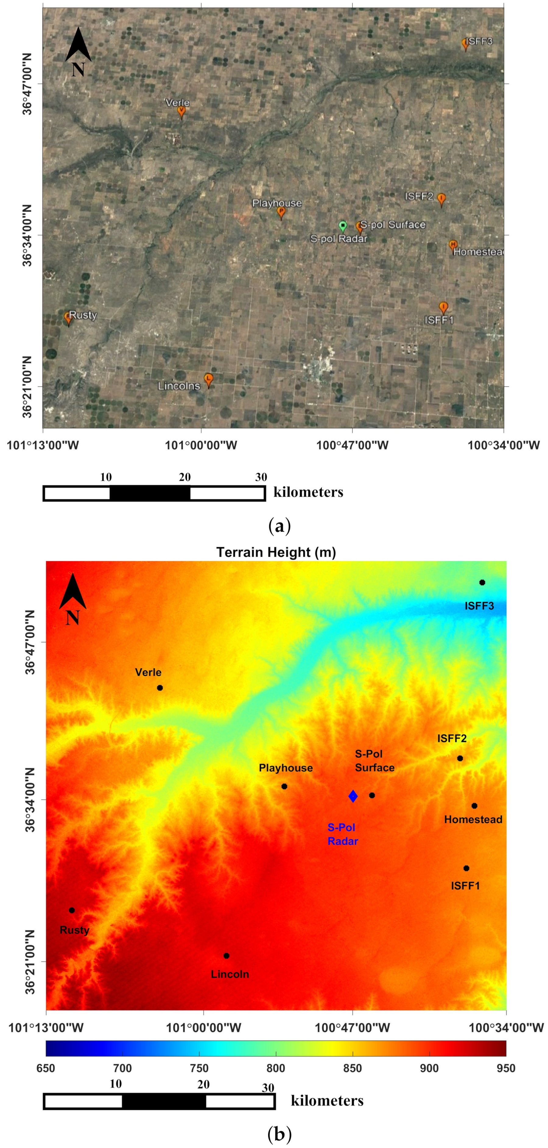
2.1. Study Area

The International H 2 O Project took place in the Southern Great Plains of the United States (Oklahoma, USA) (Figure 1a). Data from different in situ and remote sensing instruments were collected between 13 May 2002 and 25 June 2002. Although the IHOP_2002 operation domain expanded over a larger area [14], this study will be performed within the NCAR S-Pol radar coverage domain (Oklahoma panhandle). The terrain profile in this area, around the radar location ( 100 46 58 W, 36 34 15 N) and with a coverage radius of about 40–50 km ( 36 10 00 N to 37 00 00 N, 101 13 00 W to 100 34 00 W), can be considered flat since the elevation varies only between 700 m (in the northern east area crossed by the Beaver river valley) and 950 m above sea level (in the southern west area) as shown in Figure 1b.

2.2. Data Sources

Radar phase data to estimate the refractivity and the refractivity vertical gradient were collected using the S-Band Dual-Polarization Doppler Coherent Radar of the National Center for Atmospheric Research (NCAR S-Pol Radar) [26,38]. In particular, surveillance scans at an elevation angle of 0 and with a temporal resolution of approximately 5 min were obtained from 14:55 UTC (Universal Time Coordinated) on 13 May 2002 to 20:30 UTC on 25 June 2002. The scanning parameters for the S-Pol radar used during the IHOP_2002 project are summarized in Table 1.
Refractivity data to estimate the phase difference function and for the cross-validation of radar refractivity estimates were obtained from different data sources. Temperature, atmospheric pressure and water vapor pressure data were provided by six ground-based weather stations (S-Pol Surface, Verle, Lincoln, Rusty, Playhouse and Homestead) and three integrated surface flux facility (ISFF) stations (ISFF1, ISFF2 and ISFF3), deployed inside the influence area of the radar (see Figure 1a,b). These data were used to derive in-situ refractivity measurements. Indeed at microwave frequencies, the refractivity can be approximately obtained as [39]:
N = 77.6 p T + 3.73 · 10 5 e T 2
where p is the atmospheric pressure in hPa, T is the temperature in kelvin and e is the water vapor pressure in hPa. The location of the weather stations and their position with respect to the radar are summarized in Table 2.
Besides, the Atmospheric Emitted Radiance Interferometer (AERI) instrument located at the Homestead site (Figure 1b) was used to derive the vertical gradient of refractivity from the vertical structure of the temperature and the water vapor measuring the downwelling infrared radiances [40].
Additionally, the ERA5 reanalysis dataset provided by the European Centre for Medium-Range Weather Forecasts (ECMWF) was also used [41]. ERA5 data have a temporal resolution of one hour, and a spatial resolution of thirty kilometers, and resolves the atmosphere using 137 levels extending from the surface to 80 km. Temperature, humidity, and geopotential height data obtained from the lowest ERA5 pressure levels (1000 hPa, 975 hPa and 950 hPa) of nine ERA5 cells centered in the radar location were used to calculate refractivity and refractivity gradient estimates within the coverage area of the NCAR S-Pol Radar.

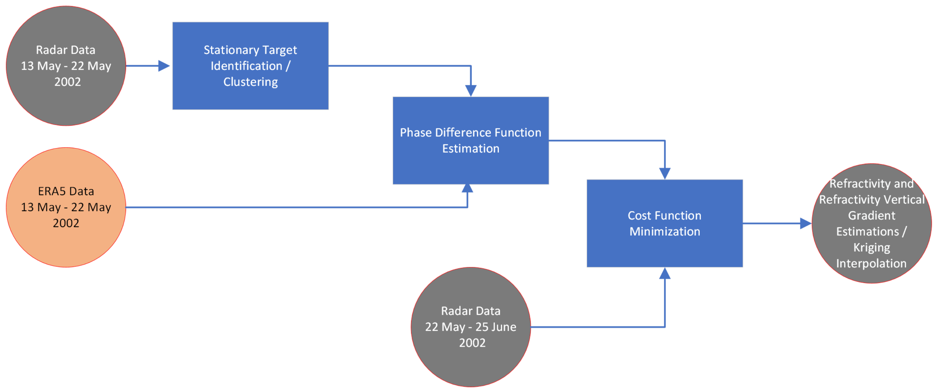
3. Radar Refractivity Algorithm

Theoretical Background

The non-linear least squares method presented in [36] to estimate simultaneously the refractivity and the refractivity vertical gradient is used in this study. The data processing flowchart to obtain radar refractivity measurements is shown in Figure 2.
This method is based on the estimation of the phase difference function corresponding to every couple of stationary targets within the radar coverage area, considering as stationary targets those targets that remain practically invariant with time [42]. The phase difference function of the k-th couple of stationary targets ( T 0 k , T 1 k ), Δ Φ T 0 k , T 1 k ( N ¯ , N h ) , is the difference between the phases of the backscattered signal from each one of the stationary targets of the couple. If a klystron-based radar, such as the NCAR S-Pol radar, is considered, the phase difference function for the k-th couple is well approximated by a linear function of the refractivity and the refractivity vertical gradient [33,35], as:
Δ Φ T 0 k , T 1 k ( N ¯ , N h ) = A k + B k N ¯ + C k N h
where A k , B k and C k are constants that depend on unknown parameters such as the range to the stationary targets, their height, or their backscattered phase. These constants are estimated from phase difference measurements at known refractivity conditions so that the phase difference function is estimated. Once the phase difference function has been estimated for all couples of stationary targets, the refractivity and the refractivity vertical gradient are determined as the values that minimize a cost function defined as the weighted sum of the sum of squares of residuals and a function of the variation of the refractivity and of the refractivity gradient from the previous measurement, that is
N ¯ , N h = arg min N ¯ , N h ( w a · k = 1 K [ ( e j Δ Φ T 0 k , T 1 k ( N ¯ , N h ) ·   e j Δ Φ T 0 k , T 1 k ( m ) ) ] 2 + ( 1 w a ) · f ( Δ N ¯ , Δ N / h ) )
where K represents the number of stationary target pairs, w a is a weight factor, Δ Φ T 0 k , T 1 k ( m ) is the phase difference measured for the m-th transmitted pulse corresponding to the k-th stationary target pair and f ( Δ N ¯ , Δ N / h ) is a function that measures the variation of the refractivity and of the refractivity vertical gradient from the previous measurement. This function is included in the cost function (Equation (3)) to avoid large errors in the estimation of N ¯ and N h that occur in noisy situations due to the "periodicities" of the sum of squares of residuals.
Using all the stationary target pairs identified within the coverage area of the radar, an estimate of the mean refractivity and an estimate of the refractivity vertical gradient over the coverage area is obtained. Figure 3 shows the mean refractivity estimated using NCAR S-Pol Radar data and the mean refractivity at the radar height estimated using the data provided by the weather stations listed in Table 2, all within the radar coverage area. The agreement between both estimates is very good, with a RMSE (Root Mean Squared Error) between both estimates of 2.18 N-units.
On the other hand, if the coverage area of the radar is divided into smaller areas or subareas, and just the stationary target pairs within each subarea are used, an estimate of the mean refractivity and an estimate of the refractivity vertical gradient over each one of the defined subareas is obtained.
Defining the subareas is not a trivial task. To ensure the accuracy and precision of refractivity estimates, these subareas must contain a sufficient number of pairs of stationary targets. They should also be as compact as possible, minimizing the dispersion of pairs of stationary targets within each subarea. Therefore, a k-means clustering algorithm has been employed to define these subareas. A total of 35 clusters have been set, so even the one with the fewest target pairs contains 94, which is a sufficient number to guarantee a good estimate of refractivity. Figure 4 shows the clusters defined.
Then, from the refractivity values estimated at each subarea radar refractivity maps can be obtained by means of interpolation. Geostatistical interpolation was used considering that the large amount of data provided by weather radars allows obtaining a good estimate of the spatial correlation of the radar refractivity. In particular, since local spatial trends of the refractivity were not observed within the area of study, Ordinary Kriging was used to produce radar refractivity maps [37]. Ordinary Kriging is a well-established and proven method, widely used in meteorology [43] as well as in other fields [44]. Assuming second-order stationarity of the data, Ordinary Kriging provides the BLUP (Best Linear Unbiased Predictor) without requiring knowledge of the mean, which, in fact, is most usually unknown [45,46].

4. Results

Radar measurements collected from 14:55 UTC on 13 May 2002 to 20:30 UTC on 25 June 2002 by the NCAR S-Pol radar are used to analyze the dryline evolution and evaluate the radar phase measurements based algorithm for obtaining refractivity maps. In particular, radar phase measurements gathered from 13 May 2002 to 22 May 2002 are used to obtain the phase difference function for each and every one of the pairs of stationary targets identified within the NCAR S-Pol radar coverage. The ERA5 reanalysis dataset is used to derive the refractivity and refractivity gradient at the time of the measurements used to obtain the phase difference function. Radar phase measurements gathered from 22 May 2002 to 25 June 2002 are used to observe the dryline development and test the algorithm. To validate the radar phase measurements based results, for the refractivity and the refractivity gradient, in-situ refractivity and refractivity vertical gradient measurements derived from the automatic weather stations, listed in Table 2, and from the AERI instrument will be used.

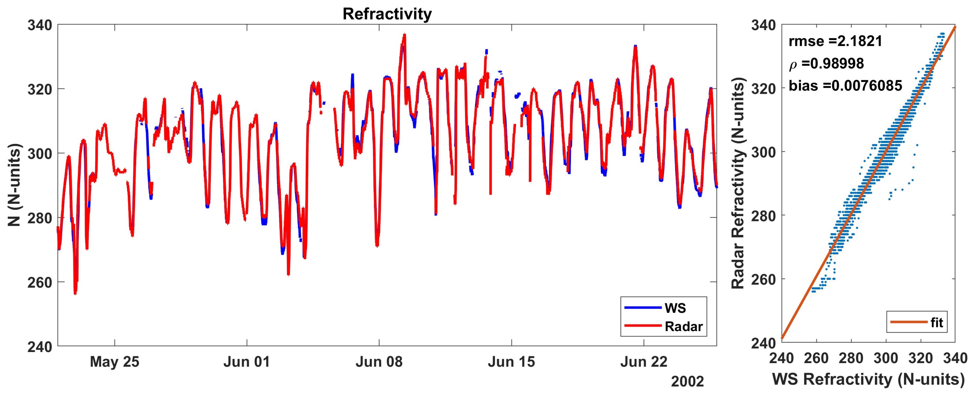
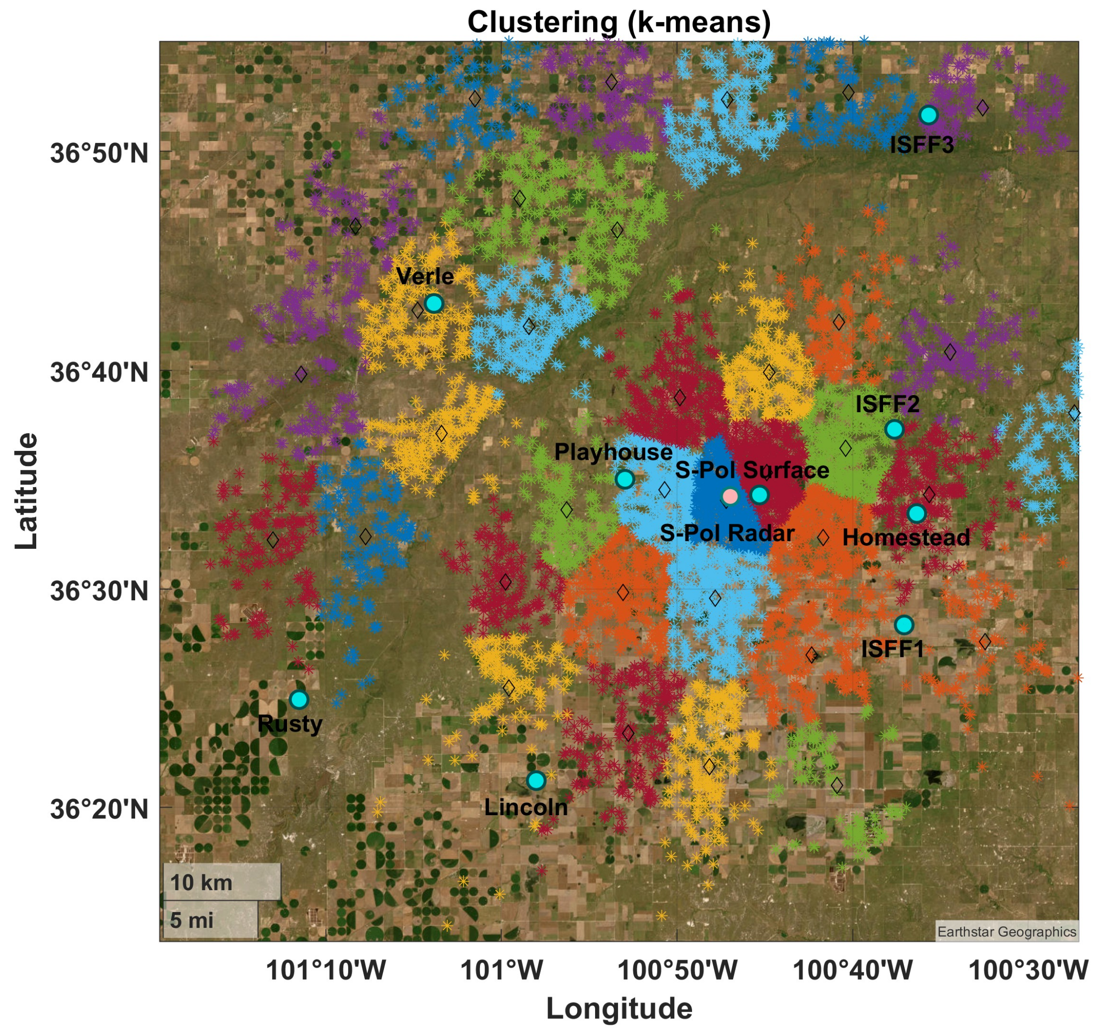
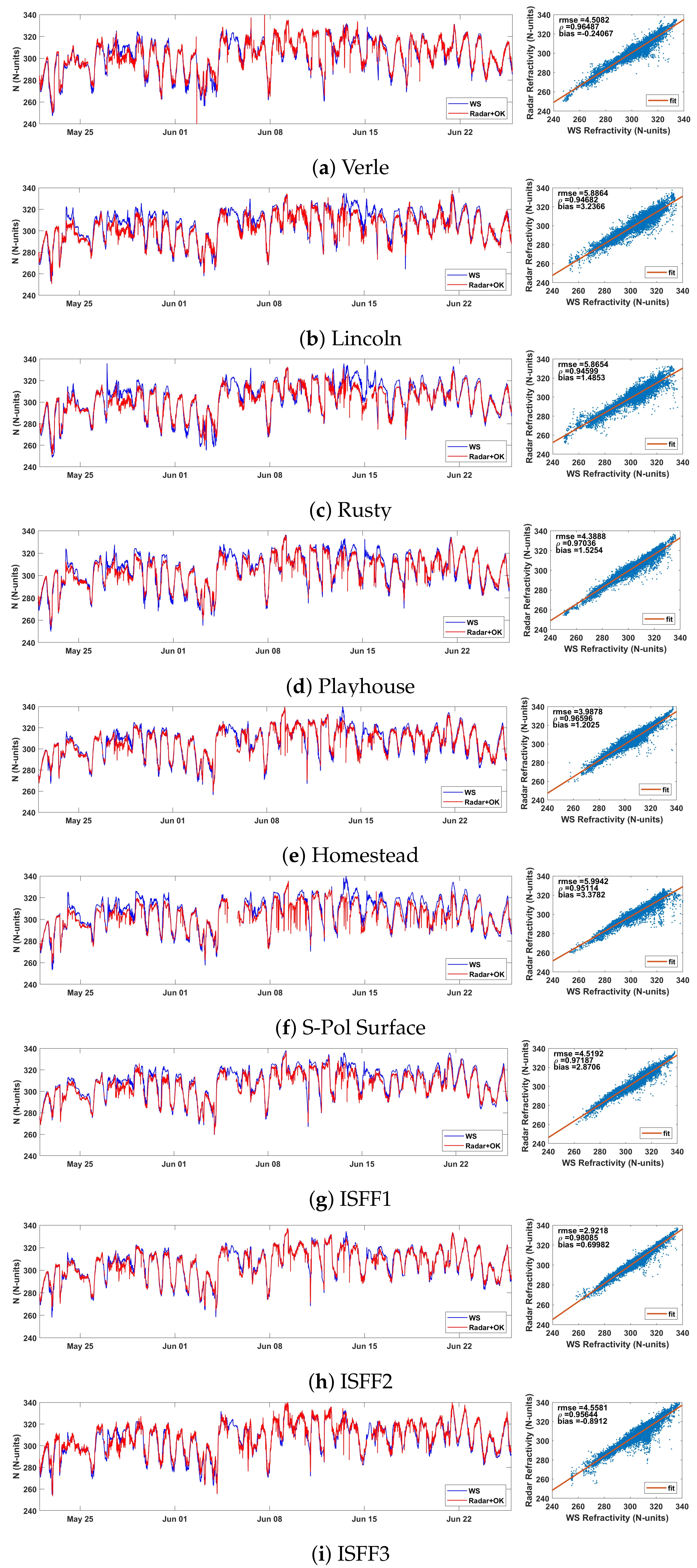
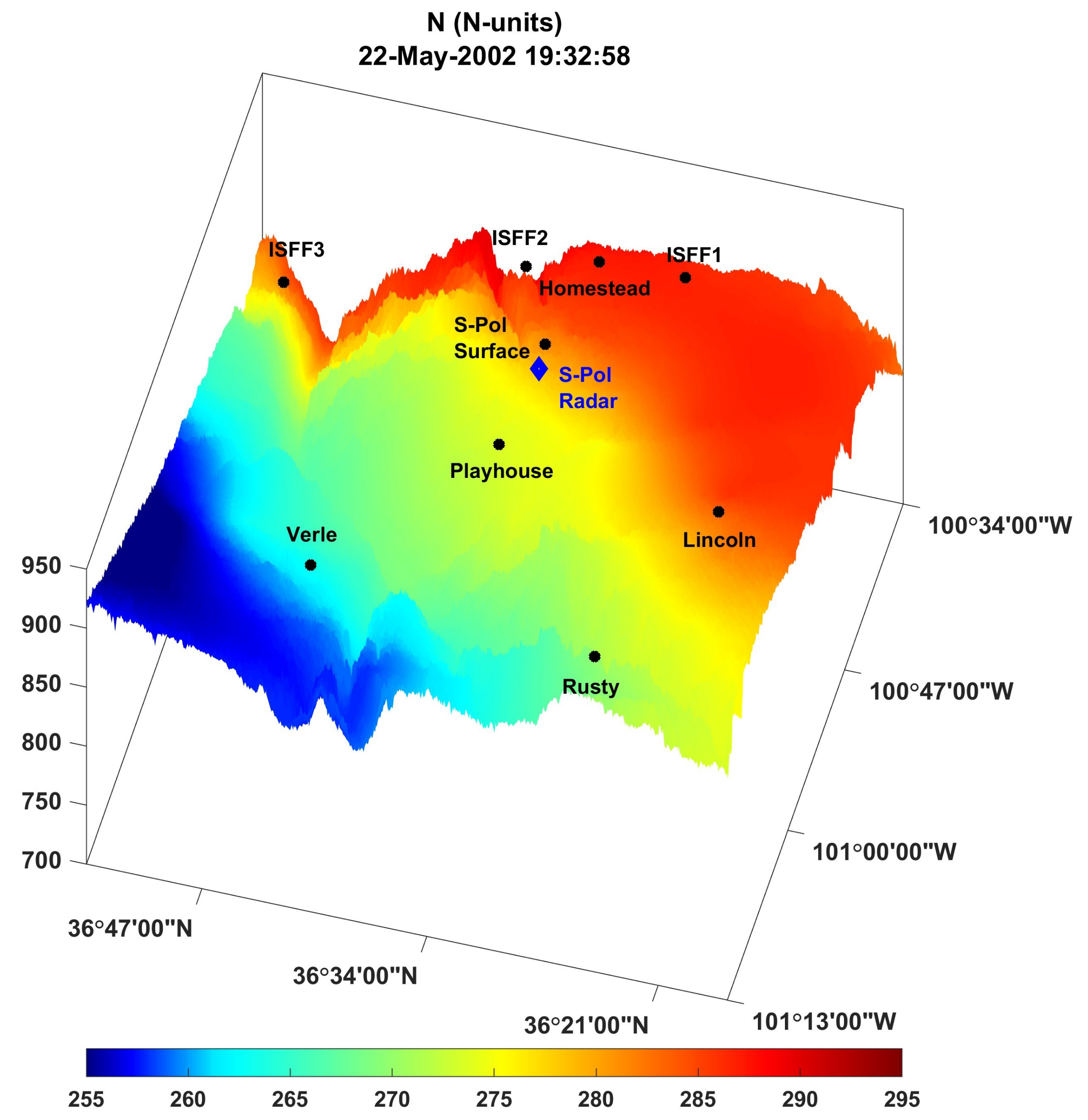
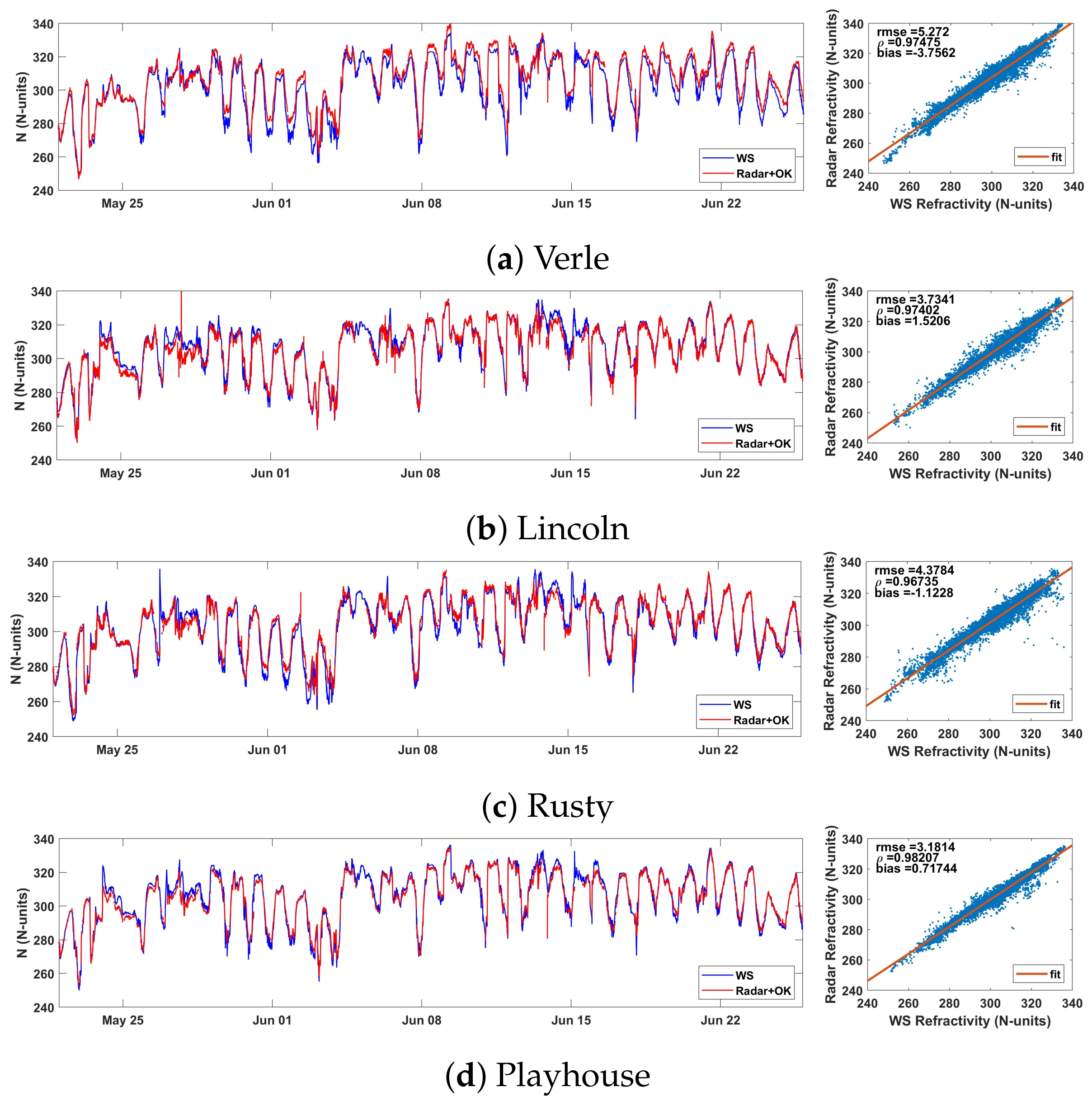
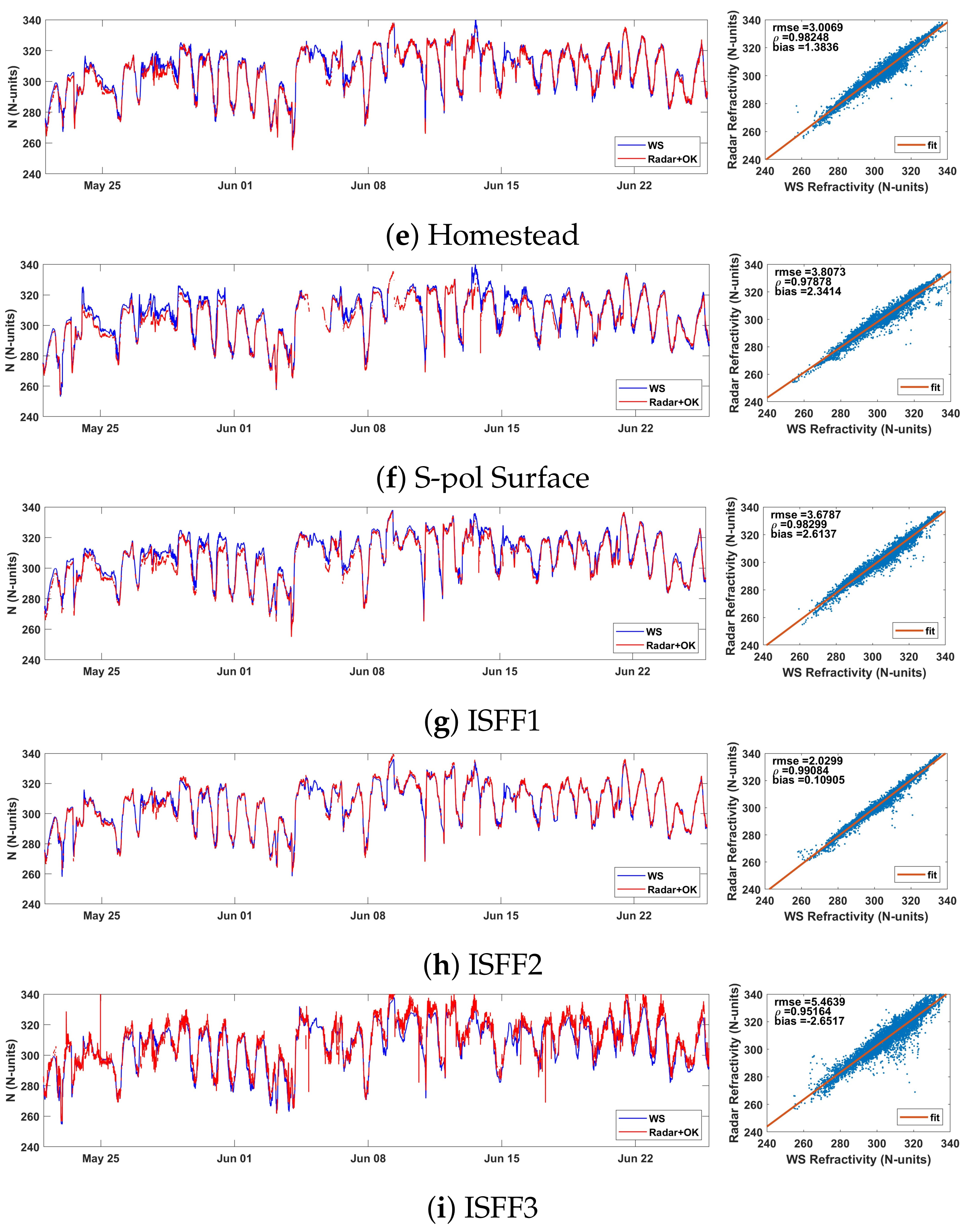
4.1. Kriging Interpolated Radar Refractivity Observations during the IHOP_2002 Project: Performance Analysis

Times series of refractivity data derived from the weather stations are compared with the kriging interpolated radar refractivity values at the weather stations location in Figure 5. Radar refractivity estimates have been calculated at the height of the weather station to be compared with. Additionally, the scatter plots of the radar refractivity estimates versus the refractivity derived from the weather station data are shown.
As can be observed in Figure 5, the kriging interpolated radar refractivity and the refractivity derived from weather station data obtained during the IHOP_2002 project show a good agreement. The correlation coefficient ρ obtained in any location of the weather stations always exceeds 0.95, reaching a high value of 0.98 at the ISFF2 weather station location. Regarding to the RMSE, its value is always less than 6 N-units for all cases, being even as low as 2.92 N-units at the ISFF2 weather station location. Note the good agreement between kriging interpolated radar refractivity and refractivity derived from weather station data taking into account the strong spatial and temporal refractivity variations reported throughout the IHOP_2002 project.
The results of the comparison between kriging interpolated radar refractivity and weather station refractivity are summarized in Table 3. RMSE, correlation coefficient and bias calculated for each pair of kriging interpolated radar refractivity and weather station refractivity show the potential of the algorithm to generate refractivity maps even for a low number of stationary targets identified in a certain area.

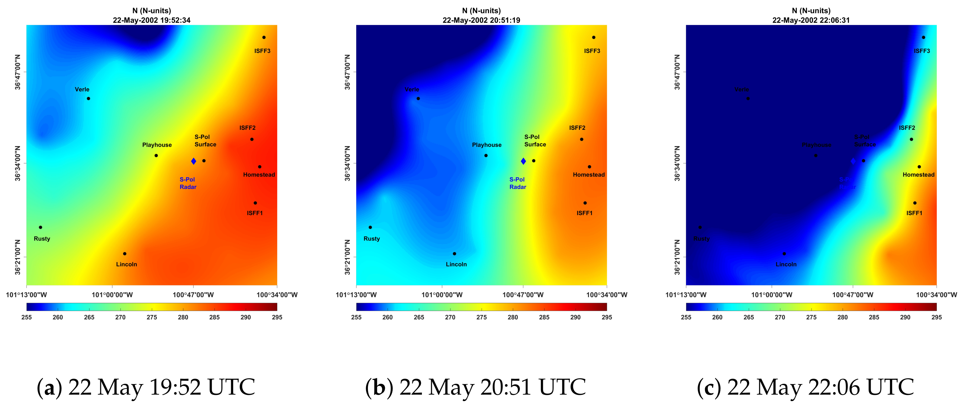
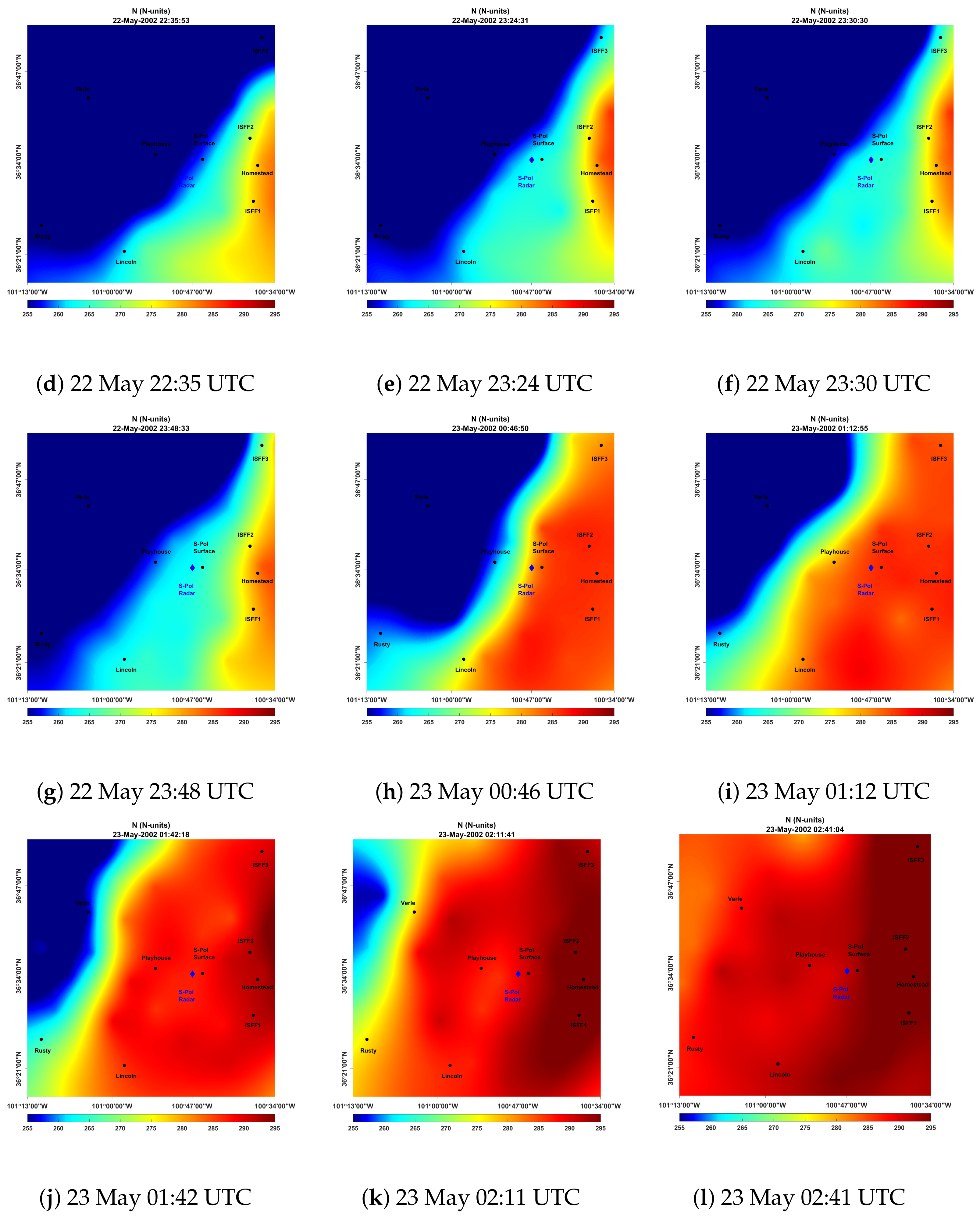
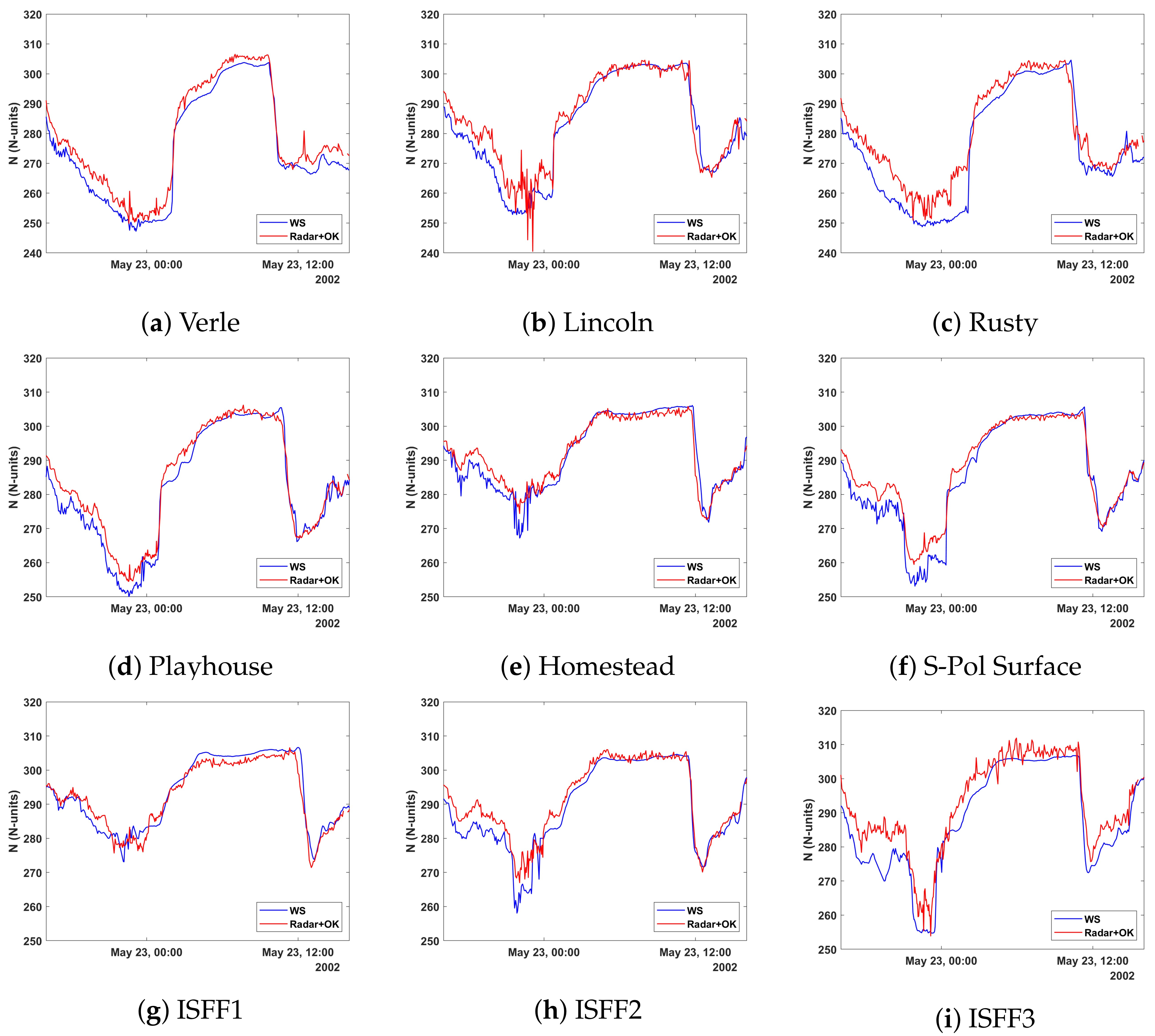
4.2. Kriging Interpolated Radar Refractivity Maps: The 22 May 2002 Dryline Evolution

Analysis of the kriging interpolated radar refractivity from 16:00 UTC on 22 May 2002 to 16:00 UTC on 23 May 2002 is of special interest. During these 24 h, a dryline developed, and the recorded refractivity at the weather stations ranged from below 250 N-units to 340 N-units, with variations in refractivity of over 30 N-units within an hour. The dryline evolution took place during the late afternoon and the early evening of 22 May 2002. In particular, Figure 6 shows several refractivity maps obtained from 19:52 UTC on 22 May to 02:41 UTC on 23 May.
As can be observed, the interpolated radar refractivity maps clearly show the temporal and spatial evolution of the dryline. At the beginning of the afternoon, the refractivity map shows a relatively uniform field (Figure 6a). As the afternoon progresses, approximately at 20:51 UTC, a significant refractivity gradient, oriented north to south through the radar can be observed (Figure 6b), i.e., the dryline is developing. The low refractivity levels of about 250–260 N-units to the west of the dryline are associated with the hot and dry air mass from the desert south-western states, while the high refractivity levels of about 280–290 N-units to the east of the dryline are associated with the warm and moist air mass from the Gulf of Mexico. Approximately at 22:06 UTC, the dryline previously identified has slightly moved towards the east, while a secondary dryline can be observed from northeast to southwest through the radar (Figure 6c). The double dryline reported by [16,21,22] on the afternoon of 22 May 2002 has formed. This double dryline is approximately observed from 22:06 UTC to 23:48 UTC (Figure 6c–g). During this time interval, the double dryline has moved very slowly towards the west of the radar. Refractivity variations on the order of 40-45 N-units can be observed inside the analysis area. However, it is worth highlighting the strong refractivity variation of approximately 20 and 10 N-units along the fine line defined by the dryline that separates the Homestead area from the radar location and the Playhouse area from the radar location, respectively. From 00:46 UTC to 02:11 UTC on 23 May, only the primary dryline can be identified (Figure 6h–k). In this time interval, the dryline has moved rapidly to the west. Finally, approximately at 02:41 UTC the dryline is no longer observed within the area of interest and the refractivity map shows again a relatively uniform field (Figure 6l).
It is worth mentioning that, unlike previous works, the refractivity maps generated by combining the non-linear least squares radar refractivity algorithm with ordinary kriging-based geostatistical interpolation techniques present reliable estimates even in locations with low target density as happens in the areas around Rusty and ISFF3 weather stations.
During the early morning of 23 May 2002, a sharp time gradient of the refractivity, higher than 30 N-units/hour, is observed at all weather stations (see Figure 7). It is worth noting the accuracy of the time detection of this significant drop by radar refractivity.
Additionally, the RMSE, the correlation coefficient and the bias between radar refractivity and weather station data-derived refractivity during these 24 h are summarized in Table 4. In general, the results obtained during this 24 h. period with high spatial and temporal variations of the refractivity are comparable to those obtained considering all estimated values from 22 May 2002 to 25 June 2002, demonstrating the good performance and potential of the kriging interpolation radar refractivity algorithm even in highly variable spatiotemporal conditions.

5. Discussion and Concluding Remarks

In this work, the ability to map out water vapor variability through kriging interpolated radar refractivity measurements has been presented and tested under highly variable conditions in the troposphere such as those occurring during the double dryline development on the afternoon and the evening of 22 May 2002 in the Great Plains of Oklahoma (United States). The kriging interpolated radar refractivity maps presented here provide an excellent view of the horizontal structure of the refractivity, which is related to vapor pressure, and of its temporal evolution. This high spatial and temporal resolution of radar refractivity measurements may allow detection of boundary layer extreme events even before they can be detected with the most traditional reflectivity and Doppler velocity methods.
The radar refractivity estimates obtained at the weather station heights show an excellent agreement with the refractivity estimates derived from the weather stations, demonstrating the potential of using the ordinary kriging geostatistical interpolation method to generate raised-relief refractivity maps. In Figure 8, a three-dimensional radar refractivity map at the surface height obtained during the IHOP_2002 project is shown.
The accuracy of the kriging interpolated radar refractivity estimates is heavily determined by the quality of the estimation of the phase difference function. The estimation of this phase difference function depends on the amount of data available since the noise in the estimates is averaged out. In this work, data from the beginning of the IHOP_2002 project (13 May 2002) until the day on which the dryline formed (22 May 2002) have been used to estimate the phase difference function. The amount of data recorded in these ten days is relatively small compared to the data available during the radar’s operational life. Therefore, the accuracy of the estimates could be significantly improved by extending the time to estimate the phase difference function, for example to several weeks. It is important to note that the data required for estimating the phase difference function are the data recorded during the operation of the radar, that is, there is no need to stop the radar in order to obtain more data to improve the estimation of the phase difference function. On the other hand, the phase difference function is estimated at known refractivity conditions, so that an independent source of data is necessary. In this paper, the ERA5 reanalysis dataset is used. Alternatively, data from the weather stations could have been used. Results, not shown here, show no significant differences when using the weather station data or the ERA5 dataset (see Figure 9). This fact is important given that some national meteorological services have stated that they will no longer expand their ground-based weather station networks due to their high cost of deployment and maintenance [31].
Finally, it is clear that there exists a trade-off between the number of stationary target pairs per subarea to ensure a local good estimate of refractivity and the total number of clusters to guarantee a good spatial resolution. The use of simple k-means has demonstrated a good performance both in accuracy and spatial resolution, but it would be of interest to develop a more exhaustive analysis to optimize the clustering of stationary target pairs.

Author Contributions

Conceptualization, V.S.d.R. and R.N.L.; methodology, V.S.d.R., R.N.L. and B.S.-R.; software, V.S.d.R., R.N.L. and B.S.-R.; validation, V.S.d.R. and R.N.L.; formal analysis, V.S.d.R., R.N.L. and B.S.-R.; investigation, V.S.d.R., R.N.L. and B.S.-R.; resources, R.N.L.; data curation, R.N.L.; writing—original draft preparation, V.S.d.R. and R.N.L.; writing—review and editing, V.S.d.R. and R.N.L.; visualization, V.S.d.R., R.N.L. and B.S.-R.; supervision, V.S.d.R.; project administration, V.S.d.R.; funding acquisition, V.S.d.R. All authors have read and agreed to the published version of the manuscript.

Funding

This work has been funded by NextGenerationEU/PRTR under project TED2021-130056B-I00.

Institutional Review Board Statement

Not applicable.

Informed Consent Statement

Not applicable.

Data Availability Statement

The ECMWF’s ERA5 dataset is available at https://doi.org/10.24381/cds.bd0915c6 (accessed on 22 April 2022). S-band radar data and related WS data were provided by NCAR/EOL under sponsorship of the National Science Foundation (website: http://data.eol.ucar.edu/) (accessed on 15 May 2021). Processing data are stored on the servers of the research group. For data requests, please contact V. Santalla del Río at [email protected].

Acknowledgments

The authors would like to thank the ECMWF and NCAR/EOL for providing open access to the radar measurements and meteorological datasets used for this work.

Conflicts of Interest

The authors declare no conflict of interest.

Abbreviations

The following abbreviations are used in this manuscript:
RMSERoot Mean Square Error
UTCUniversal Time Coordinated
NCARNational Center for Atmospheric Research
ISFFIntegrated Surface Flux Facility
AERIAtmospheric Emitted Radiance Interferometer
IHOPInternational H 2 O Project
ECMWFEuropean Centre for Medium-Range Weather Forecast
ERA5ECMWF reanalysis v5
NWPNumerical Weather Prediction

References

  1. Fujita, T. Structure and Movement of a Dry Front. Bull. Am. Meteorol. Soc. 1958, 39, 574–582. [Google Scholar] [CrossRef]
  2. Rhea, J.O. A Study of Thunderstorm Formation Along Dry Lines. J. Appl. Meteorol. Climatol. 1966, 5, 58–63. [Google Scholar] [CrossRef]
  3. Ziegler, C.L.; Rasmussen, E.N. The Initiation of Moist Convection at the Dryline: Forecasting Issues from a Case Study Perspective. Weather Forecast. 1998, 13, 1106–1131. [Google Scholar] [CrossRef]
  4. Ziegler, C.L.; Lee, T.J.; Pielke, R.A. Convective initiation at the dryline: A modeling study. Mon. Weather Rev. 1997, 125, 1001–1026. [Google Scholar] [CrossRef]
  5. Parsons, D.B.; Shapiro, M.A.; Miller, E. The Mesoscale Structure of a Nocturnal Dryline and of a Frontal–Dryline Merger. Mon. Weather Rev. 2000, 128, 3824–3838. [Google Scholar] [CrossRef]
  6. Crook, N.A. Sensitivity of moist convection forced by boundary layer processes to low-level thermodynamic fields. Mon. Weather Rev. 1996, 124, 1767–1785. [Google Scholar] [CrossRef]
  7. Weckwerth, T.M.; Wilson, J.W.; Wakimoto, R.M. Thermodynamic Variability within the Convective Boundary Layer due to Horizontal Convective Rolls. Mon. Weather Rev. 1996, 124, 769–784. [Google Scholar] [CrossRef]
  8. Sun, J. Convective-scale assimilation of radar data: Progress and challenges. Q. J. R. Meteorol. Soc. 2005, 131, 3439–3463. [Google Scholar] [CrossRef]
  9. Gasperoni, N.A.; Xue, M.; Palmer, R.D.; Gao, J. Sensitivity of Convective Initiation Prediction to Near-Surface Moisture When Assimilating Radar Refractivity: Impact Tests Using OSSEs. J. Atmos. Ocean. Technol. 2013, 30, 2281–2302. [Google Scholar] [CrossRef]
  10. Ciesielski, P.E.; Johnson, R.H.; Haertel, P.T.; Wang, J. Corrected TOGA COARE Sounding Humidity Data: Impact on Diagnosed Properties of Convection and Climate over the Warm Pool. J. Clim. 2003, 16, 2370–2384. [Google Scholar] [CrossRef]
  11. Kuo, Y.H.; Sokolovskiy, S.V.; Anthes, R.A.; Vandenberghe, F. Assimilation of GPS radio occultation data for numerical weather prediction. Terr. Atmos. Ocean. Sci. 2000, 11, 157–186. [Google Scholar] [CrossRef]
  12. Bevis, M.; Businger, S.; Herring, T.A.; Rocken, C.; Anthes, R.A.; Ware, R.H. GPS Meteorology: Remote Sensing of Atmospheric Water Vapor Using the Global Positioning System. J. Geophys. Res. 1992, 97, 15787–15801. [Google Scholar] [CrossRef]
  13. UCAR/ATD. International H2O Project (IHOP_2002): Operations Plan. 2002. Available online: https://www.eol.ucar.edu/field_projects/ihop2002 (accessed on 12 December 2023).
  14. Weckwerth, T.M.; Parson, D.B.; Koch, S.E.; Moore, J.A.; LeMone, L.M.; Demoz, B.B.; Flamant, C.; Geerts, B.; Wang, J.; Feltz, W.F. An overview of the International H2O Project (IHOP_2002) and some preliminary highlights. Bull. Am. Meteorol. Soc. 2004, 85, 253–277. [Google Scholar] [CrossRef]
  15. Demoz, B.; Miller, D.; di Girolamo, P.; Whiteman, D.; Evans, K.; Flamant, C.; Geerts, B.; Weckwerth, T.; Starr, D.; Schwemmer, G.; et al. The 22 may Dryline in IHOP2002: The Role of Lidars in Quantifying the Convective Variability. In Proceedings of the 22nd Internation Laser Radar Conference (ILRC 2004), Matera, Italy, 12–16 July 2004; ESA Special Publication. Pappalardo, G., Amodeo, A., Eds.; Volume 561, p. 739. [Google Scholar]
  16. Demoz, B.B.; Flamant, C.; Weckwerth, T.M.; Whiteman, D.; Evans, K.; Fabry, F.; Girolamo, P.; Miller, D.; Geerts, B.; Brown, W.; et al. The Dryline on 22 May 2002 during IHOP_2002: Convective-Scale Measurements at the Profiling Site. Mon. Weather Rev. 2006, 134, 294–310. [Google Scholar] [CrossRef]
  17. Weldegaber, M.H.; Demoz, B.B.; Sparling, L.C.; Hoff, R.; Chiao, S. Observational analysis of moisture evolution and variability in the boundary layer during the dryline on 22 May 2002. Meteorol. Atmos. Phys. 2010, 110, 87–102. [Google Scholar] [CrossRef]
  18. Weckwerth, T.M.; Parsons, D.B. A review of Convection Initiation and Motivation for IHOP_2002. Mon. Weather Rev. 2006, 134, 5–22. [Google Scholar] [CrossRef]
  19. Wakimoto, R.M.; Murphey, H.V.; Browell, E.V.; Ismail, S. The Triple Point on 24 May 2002 during IHOP. Part I: Airborne Doppler and LASE Analyses of the Frontal Boundaries and Convection Initiation. Mon. Weather Rev. 2006, 134, 231–250. [Google Scholar] [CrossRef]
  20. Cai, H.; Lee, W.C.; Weckwerth, T.M.; Flamant, C.; Murphey, H.V. Observations of the 11 June Dryline during IHOP_2002—A Null Case for Convection Initiation. Mon. Weather Rev. 2006, 134, 336–354. [Google Scholar] [CrossRef]
  21. Weckwerth, T.M.; Pettet, C.R.; Fabry, F.; Park, S.; LeMone, M.A.; Wilson, J.W. Radar refractivity retrieval: Validation and application to short-term forecasting. J. Appl. Meteorol. 2005, 44, 285–300. [Google Scholar] [CrossRef]
  22. Weiss, C.C.; Bluestein, H.B.; Pazmany, A.L. Finescale Radar Observations of the 22 May 2002 Dryline during the International H2O Project (IHOP). Mon. Weather Rev. 2006, 134, 273–293. [Google Scholar] [CrossRef]
  23. Wakimoto, R.M.; Murphey, H.V. Frontal and Radar Refractivity Analyses of the Dryline on 11 June 2002 during IHOP. Mon. Weather Rev. 2010, 138, 228–241. [Google Scholar] [CrossRef]
  24. Fabry, F.; Frush, C.; Zawadzki, I.; Kilambi, A. On the extraction of near-surface index of refraction using radar phase measurements from ground targets. J. Atmos. Ocean. Technol. 1997, 14, 978–987. [Google Scholar] [CrossRef]
  25. Fabry, F. Meteorological Value of Ground Target Measurements. J. Atmos. Ocean. Technol. 2004, 21, 560–573. [Google Scholar] [CrossRef]
  26. Lutz, J.P.; Lewis, E.; Loew, E.; Randall, M.; Van Andel, J. NCAR SPol: Portable polarimetric S-Band radar. In Proceedings of the Ninth Symposium on Meteorological Observations and Instrumentation, Charlotte, NC, USA, 27–31 March 1995; pp. 408–410. [Google Scholar] [CrossRef]
  27. Fabry, F. The Spatial Variability of Moisture in the Boundary Layer and its Effect on Convection Initiation: Project-Long Characterization. Mon. Weather Rev. 2006, 134, 978–987. [Google Scholar] [CrossRef]
  28. Buban, M.S.; Ziegler, C.L.; Rasmussen, E.N.; Richardson, Y.P. The Dryline on 22 May 2002 during IHOP: Ground-Radar and In Situ Data Analyses of the Dryline and Boundary Layer Evolution. Mon. Weather Rev. 2007, 135, 2473–2505. [Google Scholar] [CrossRef]
  29. Roberts, R.D.; Fabry, F.; Kennedy, P.C.; Nelson, E.; Wilson, J.; Rehak, N.; Fritz, J.; Chandrasekar, V.; Braun, J.; Sun, J.; et al. REFRACTT_2006: Real-Time retrieval of high-resolution low-level moisture fields from operational NEXRAD and research radars. Bull. Am. Meteorol. Soc. 2008, 89, 1535–1548. [Google Scholar] [CrossRef]
  30. Bodine, D.; Heinselman, P.L.; Cheong, B.L.; Palmer, R.D.; Michaud, D. A Case Study on the Impact of Moisture Variability on Convection Initiation Using Radar Refractivity Retrievals. J. Appl. Meteorol. Climatol. 2010, 49, 1766–1778. [Google Scholar] [CrossRef]
  31. Besson, L.; Caumont, O.; Goulet, L.; Bastin, S.; Menut, L.; Bresson, E.; Fourrie, N.; Fabry, F.; Parent du Chatelet, J. Comparison of real-time refractivity measurements by radar with automatic weather stations, AROME-WMED and WRF forecast simulations during SOP1 of the HyMeX campaign. Q. J. R. Meteorol. Soc. 2016, 142, 138–152. [Google Scholar] [CrossRef]
  32. Feng, Y.C.; Hsu, H.W.; Weckwerth, T.M.; Lin, P.L.; Liou, Y.C.; Wang, T.C.C. The Spatiotemporal Characteristics of Near-Surface Water Vapor in a Coastal Region Revealed from Radar-Derived Refractivity. Mon. Weather Rev. 2021, 149, 2853–2873. [Google Scholar] [CrossRef]
  33. Park, S.; Fabry, F. Simulation and interpretation of the phase data used by radar refractivity retrieval algorithm. J. Atmos. Ocean. Technol. 2010, 27, 1286–1301. [Google Scholar] [CrossRef]
  34. Feng, Y.; Fabry, F.; Weckwerth, T.M. Improving Radar Refractivity Retrieval by considering the change in the Refractivity Profile and the Varying Altitudes of Ground Targets. J. Atmos. Ocean. Technol. 2016, 33, 989–1004. [Google Scholar] [CrossRef]
  35. Nocelo, R.; Santalla, V. High Temporal Resolution Refractivity Retrieval from Radar Phase Measurements. Remote Sens. 2018, 10, 896. [Google Scholar] [CrossRef]
  36. Nocelo López, R.; Sánchez-Rama, B.; Santalla del Río, V.; Barbosa, S.; Narciso, P.; Pérez-Santalla, R.; Pettazzi, A.; Pinto, P.; Salsón, S.; Viegas, T. Refractivity and Refractivity Gradient Estimation From Radar Phase Data: A Least Squares Based Approach. IEEE Trans. Geosci. Remote Sens. 2023, 61, 5103214. [Google Scholar] [CrossRef]
  37. Sánchez-Rama, B.; Nocelo López, R.; Santalla Del Río, V.; Darlington, T. Radar-Based Refractivity Maps Using Geostatistical Interpolation. IEEE Geosci. Remote Sens. Lett. 2023, 20, 1–5. [Google Scholar] [CrossRef]
  38. UCAR/NCAR-Earth Observing Laboratory. S-Band/Ka-Band Polarimetric (S-PolKa) Data cfRadial Format, Version 1.0; UCAR/NCAR-Earth Observing Laboratory: Boulder, CO, USA, 1996; Retrieved 11 January 2015. [Google Scholar] [CrossRef]
  39. Bean, B.R.; Dutton, E.J. Radio Meteorology. Natl. Bur. Stand. Monogr. N. Y. Dover. 1968, 92, 435. [Google Scholar] [CrossRef]
  40. Feltz, W.F.; Howell, H.B.; Knuteson, R.O.; Woolf, H.M.; Revercomb, H.E. Near continuous profiling of temperature, moisture and atmospheric stability using the Atmospheric Emitted Radiance Interferometer (AERI). J. Appl. Meteorol. 2003, 42, 584–597. [Google Scholar] [CrossRef]
  41. Hersbach, H.; Bell, B.; Berrisford, P.; Hirahara, S.; Horányi, A.; Muñoz-Sabater, J.; Nicolas, J.; Peubey, C.; Radu, R.; Schepers, D.; et al. The ERA5 global reanalysis. Q. J. R. Meteorol. Soc. 2020, 146, 1999–2049. [Google Scholar] [CrossRef]
  42. Cheong, B.L.; Palmer, R.; Curtis, C.D.; Yu, T.Y.; Zrnic, D.S.; Forsyth, D. Refractivity Retrieval Using the Phased-Array Radar: First Results and Potential for Multimission Operation. IEEE Trans. Geosci. Remote Sens. 2008, 46, 2527–2537. [Google Scholar] [CrossRef]
  43. Chen, S.; Guo, J. Spatial interpolation techniques: Their applications in regionalizing climate-change series and associated accuracy evaluation in Northeast China. Geomat. Nat. Hazards Risk 2017, 8, 689–705. [Google Scholar] [CrossRef]
  44. Li, J.; Heap, A.D. A review of comparative studies of spatial interpolation methods in environmental sciences: Performance and impact factors. Ecol. Inform. 2011, 6, 228–241. [Google Scholar] [CrossRef]
  45. Webster, R.; Oliver, M.A. Geostatistics for Environmental Scientists; John Wiley & Sons: Hoboken, NJ, USA, 2007. [Google Scholar] [CrossRef]
  46. Wackernagel, H. Multivariate Geostatistics: An Introduction with Applications; Springer Science & Business Media: Berlin/Heidelberg, Germany, 2003. [Google Scholar] [CrossRef]
Figure 1. S-Pol radar coverage domain in the Southern Great Plains of United States (Oklahoma, United States): (a) Google Earth TM image centered in the S-Pol radar; (b) Topographic map of the terrain (National Elevation Dataset of the U. S. Geological Survey (USGS)).
Atmosphere 15 00033 g001
Figure 2. The data processing flowchart to obtain radar refractivity measurements.
Atmosphere 15 00033 g002
Figure 3. Mean refractivity estimates from NCAR S-Pol Radar phase measurements compared to refractivity estimates from WS measurements at the radar height. Blue dots represent the scatterplot of the radar refractivity estimates and the refractivity derived from the weather stations.
Atmosphere 15 00033 g003
Figure 4. Clusters of stationary target pairs defined with a k-means clustering algorithm within the coverage area of the NCAR S-Pol radar.
Atmosphere 15 00033 g004
Figure 5. Time series (left) and scatterplot (right) of kriging interpolated radar refractivity compared with weather station refractivity. ERA5 data are used to obtain the phase difference function.
Atmosphere 15 00033 g005
Figure 6. Refractivity maps showing the evolution of the dryline on 22 May 2002.
Atmosphere 15 00033 g006aAtmosphere 15 00033 g006b
Figure 7. Radar refractivity and weather station data derived refractivity at the weather station locations from 16:00 UTC 22 May to 16:00 UTC 23 May 2002.
Atmosphere 15 00033 g007
Figure 8. Raised-relief refractivity map from NCAR S-Pol Radar phase measurements at the surface height.
Atmosphere 15 00033 g008
Figure 9. Time series (left) and scatterplot (right) of kriging interpolated radar refractivity compared with weather stations refractivity. Weather station data are used to obtain the phase difference function.
Atmosphere 15 00033 g009aAtmosphere 15 00033 g009b
Table 1. S-Pol Radar scanning parameters during the IHOP_2002 project.
ParameterValue
Frequency2.8 GHz
Wavelength10 cm
Pulse-width0.994 μ s
Pulse repetition frequency (PRF)960 Hz
Range resolution150 m
Beam width0.918
Scan-rate8.0/8.8/13.7 /s
Samples110/100/64
Scanning elevation angle0
Noise Power−114 dBm
Table 2. Geographical coordinates, elevation above sea level and relative polar coordinates to the S-Pol radar. Azimuth is measured with respect to the north of the radar.
StationLongitudeLatitudeAltitude (m)Distance (km)Azimuth ( )
S-Pol Radar100 46 58 W36 34 15 N875
S-Pol Surface100 49 58 W36 34 19 N8832.589.44
Verle101 03 50 W36 43 04 N86229.9302.8
Lincoln100 58 01 W36 21 14 N91529.3214.1
Rusty101 11 31 W36 24 57 N92240.43244.5
Playhouse100 52 58 W36 35 02 N8769.05278.3
Homestead100 36 21 W36 33 28 N86215.8895.6
ISFF1100 37 04 W36 28 22 N87218.33126.5
ISFF2100 37 37 W36 37 19 N85915.0367.7
ISFF3100 35 40 W36 51 39 N78036.3727.5
Table 3. RMSE, correlation coefficient and bias of kriging interpolated radar refractivity versus weather station data derived refractivity at the locations of the weather stations, from 22 May 2002 to 25 June 2002.
WeatherRMSE ρ Bias
Station(N-Units) (N-Units)
Verle4.510.96−0.24
Lincoln5.880.953.24
Rusty5.860.951.48
Playhouse4.390.971.52
Homestead3.990.971.20
S-Pol Surface5.990.953.38
ISFF14.520.972.87
ISFF22.920.980.70
ISFF34.560.96−0.89
Table 4. RMSE, correlation coefficient and bias at the locations of the weather stations from 16:00 UTC on 22 May 2002 to 16:00 UTC on 23 May 2002.
WeatherRMSE ρ Bias
Station(N-Units) (N-Units)
Verle4.200.99−3.67
Lincoln5.480.96−2.69
Rusty6.930.97−4.19
Playhouse3.570.99−2.34
Homestead3.180.96−0.87
S-Pol Surface4.060.98−2.48
ISFF12.690.970.68
ISFF23.930.98−2.48
ISFF36.130.97−4.69
Disclaimer/Publisher’s Note: The statements, opinions and data contained in all publications are solely those of the individual author(s) and contributor(s) and not of MDPI and/or the editor(s). MDPI and/or the editor(s) disclaim responsibility for any injury to people or property resulting from any ideas, methods, instructions or products referred to in the content.

