
Explainable Boosting Machine: A Contemporary Glass-Box Strategy for the Assessment of Wind Shear Severity in the Runway Vicinity Based on the Doppler Light Detection and Ranging Data


Abstract
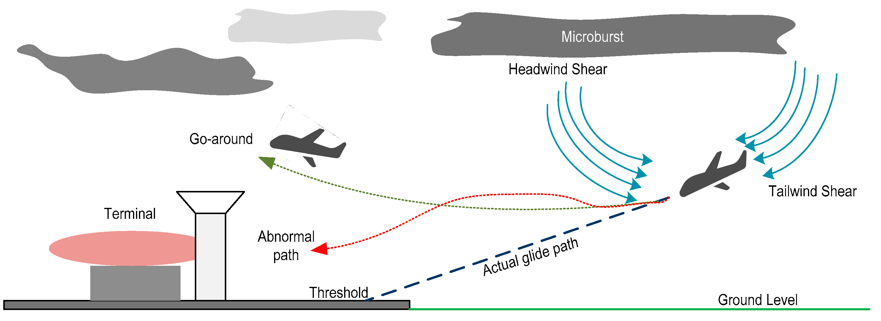
:1. Introduction
2. Materials and Methods
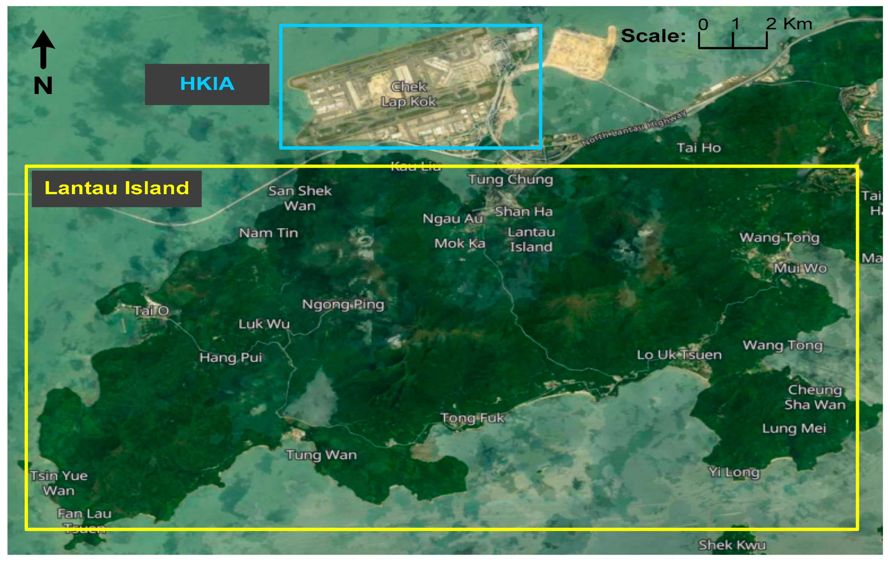
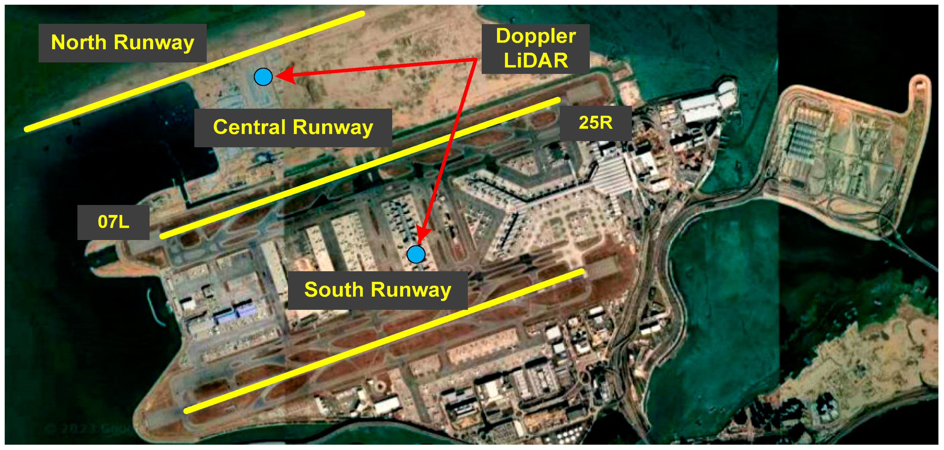
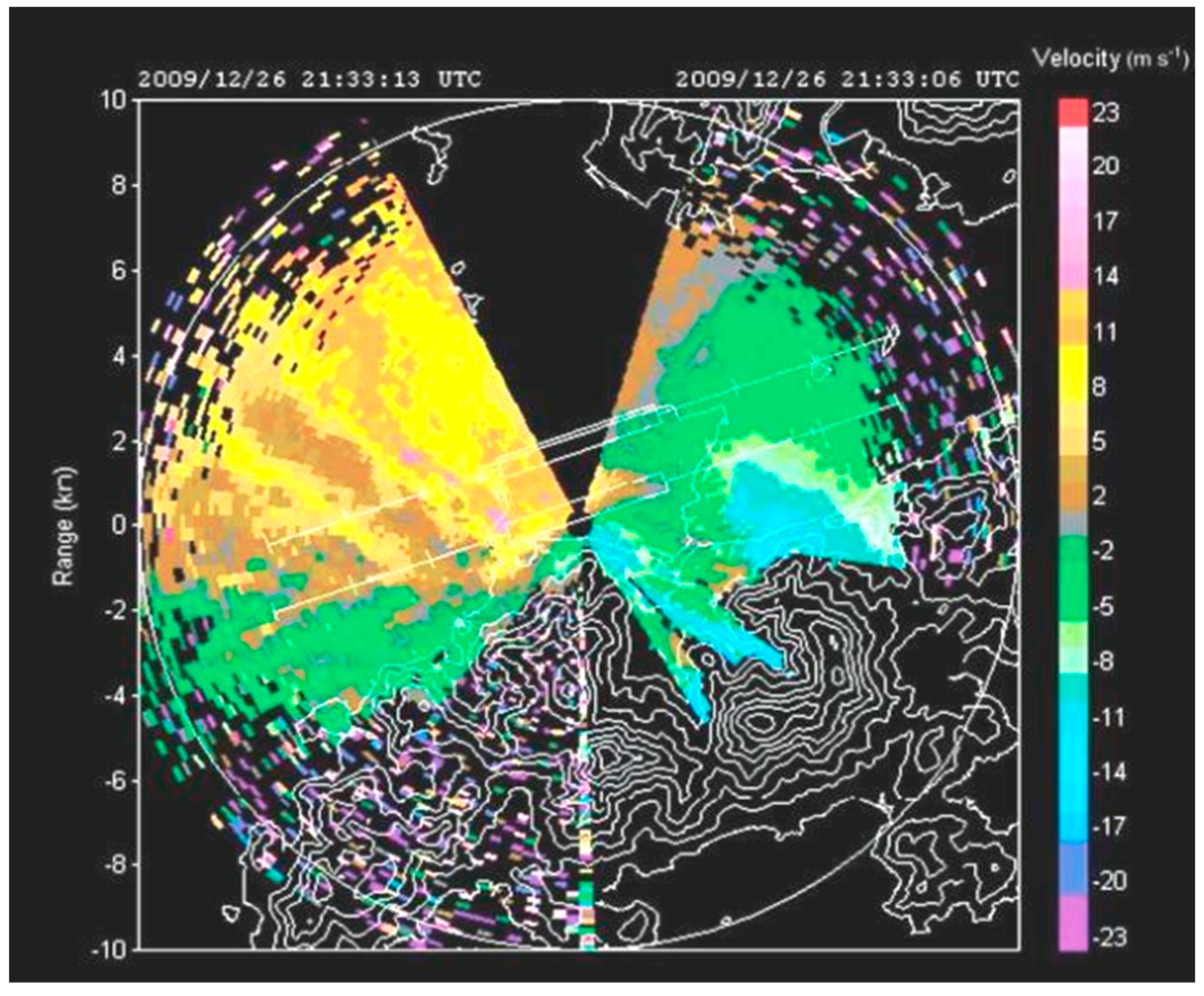
2.1. Study Location and Data Retrieval from HKIA-Based Doppler LiDAR
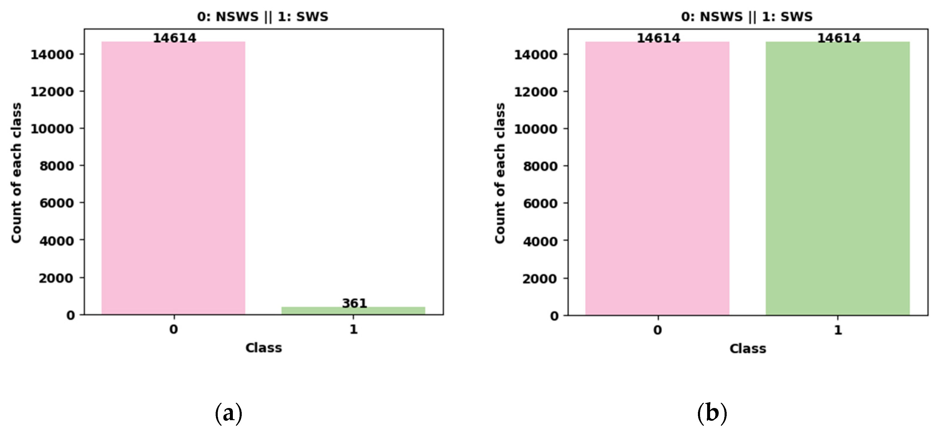
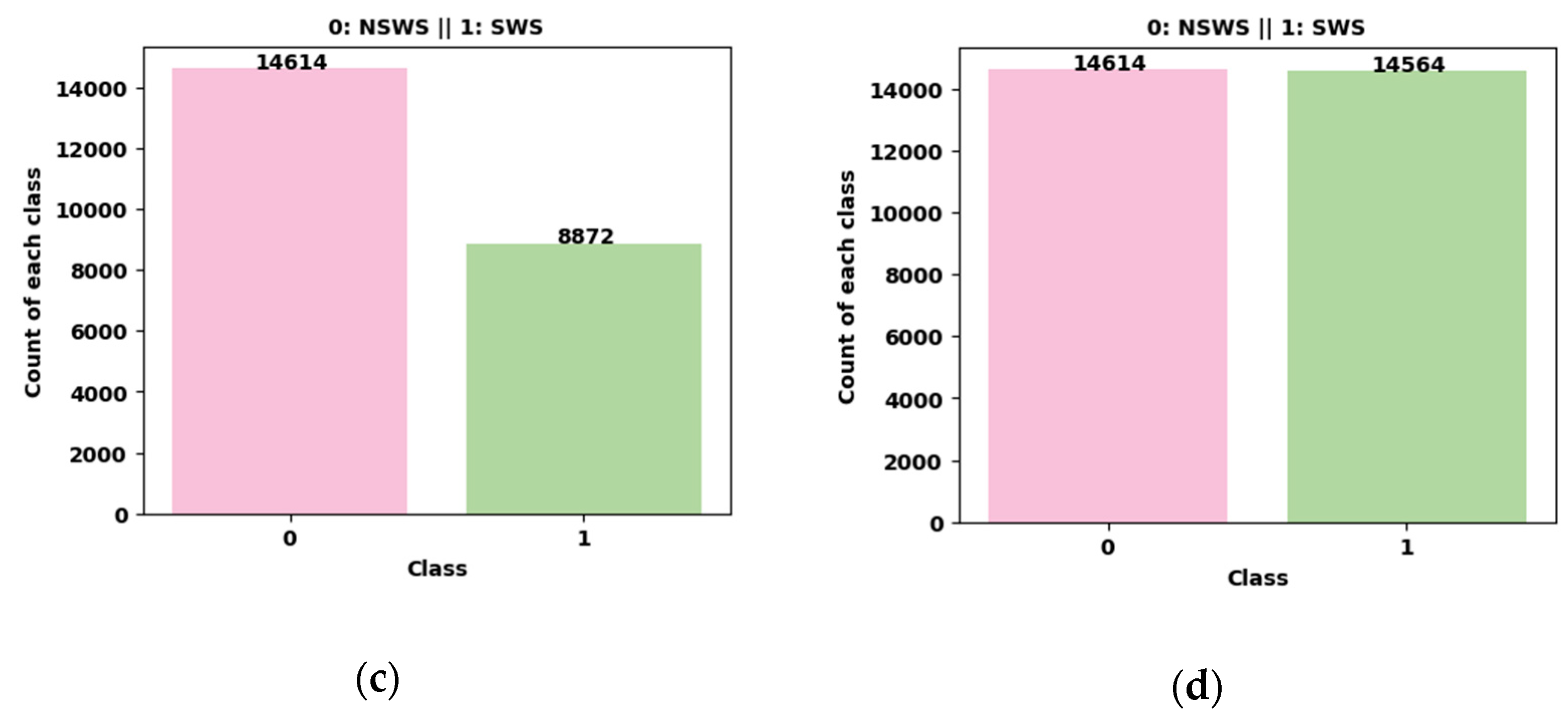
2.2. Developing a Binary Classification Problem
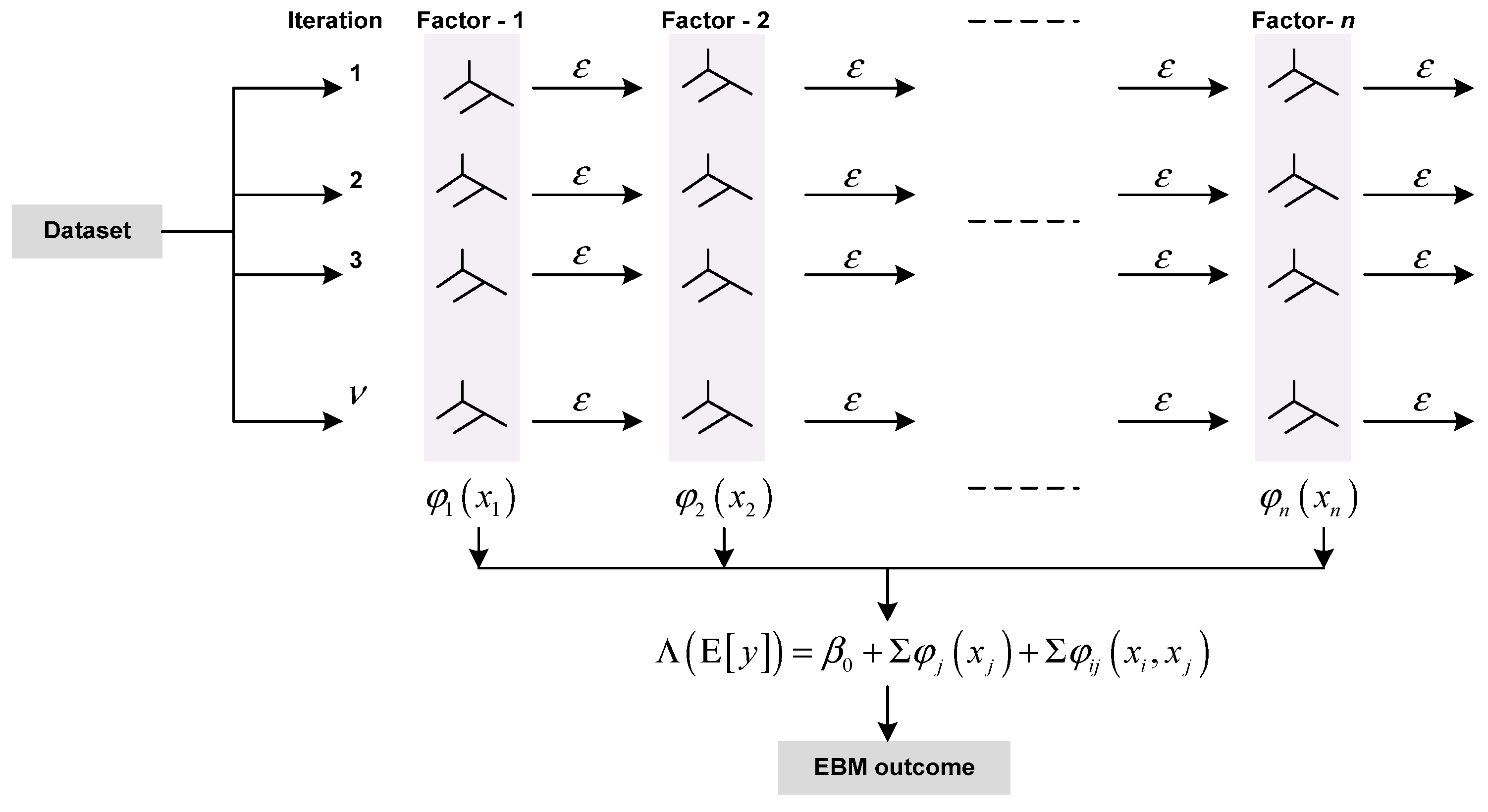
2.3. Explainable Boosting Machine: An ML-Based Glass-Box Model
- : Link function, representing identity function for regression and logit function for classification
- Intercept term
- Shape or smooth function
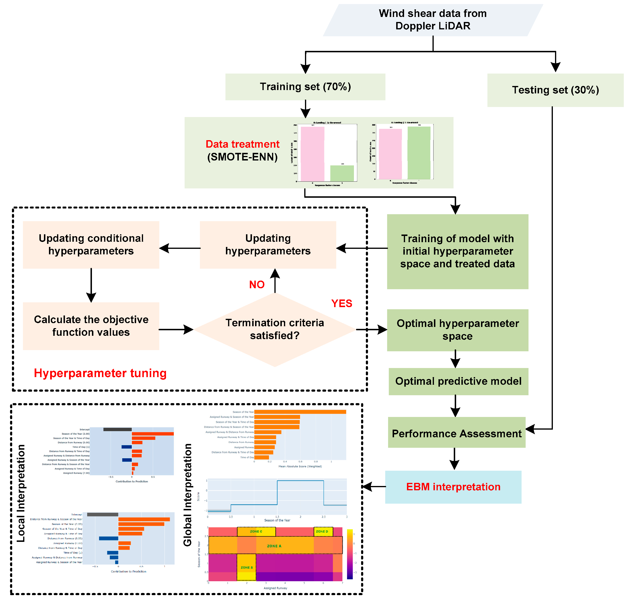
2.4. Bayesian Optimization
- First, the Bayesian optimization attempts to construct a surrogate function for by randomly selecting a subset of data points. In this study, the surrogate function was updated using a Gaussian process (GP) to create the posterior distribution over . The use of GP was justified by its high flexibility, robustness, accuracy, and analytical traceability.
- Initially, the Bayesian optimization procedure endeavors to create a surrogate function for the target function, denoted as , by employing a random selection process to choose a subset of data points. The surrogate function in this study was enhanced through the utilization of GP in order to generate the posterior distribution over . The utilization of GP was justified due to its notable attributes such as high flexibility, robustness, accuracy, and analytical traceability. Subsequently, the posterior distribution obtained from the initial step is employed to derive an acquisition function that serves the dual purpose of exploring unexplored regions within the search space and exploiting regions that have already been identified as yielding optimal outcomes. The processes of exploration and exploitation are ongoing, and the surrogate model continues to be updated with new findings until an established until the termination criterion is met. The primary aim is to enhance the performance of the acquisition function, particularly the expected improvement metric, for the purpose of identifying the subsequent sampling point.
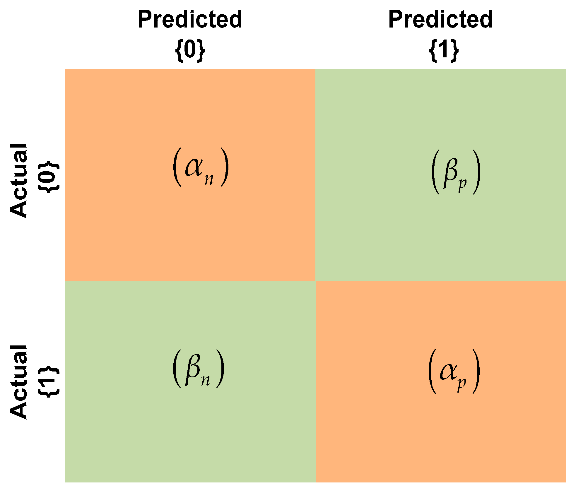
2.5. Performance Measures
3. Results and Discussion
3.1. Optimal Hyperparameters via Bayesian Optimization
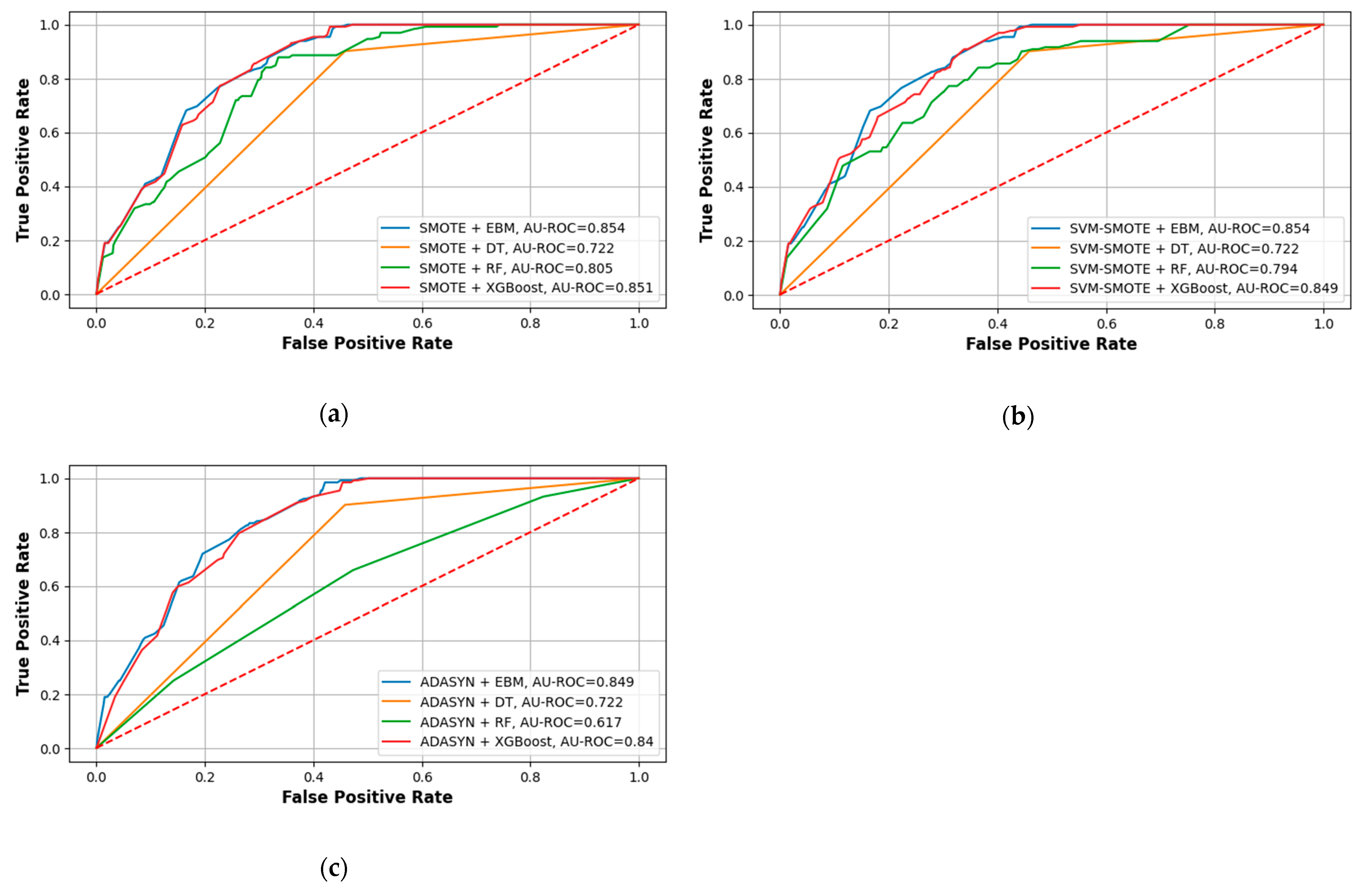
3.2. Predictive Performance of EBM and Comparative Analysis
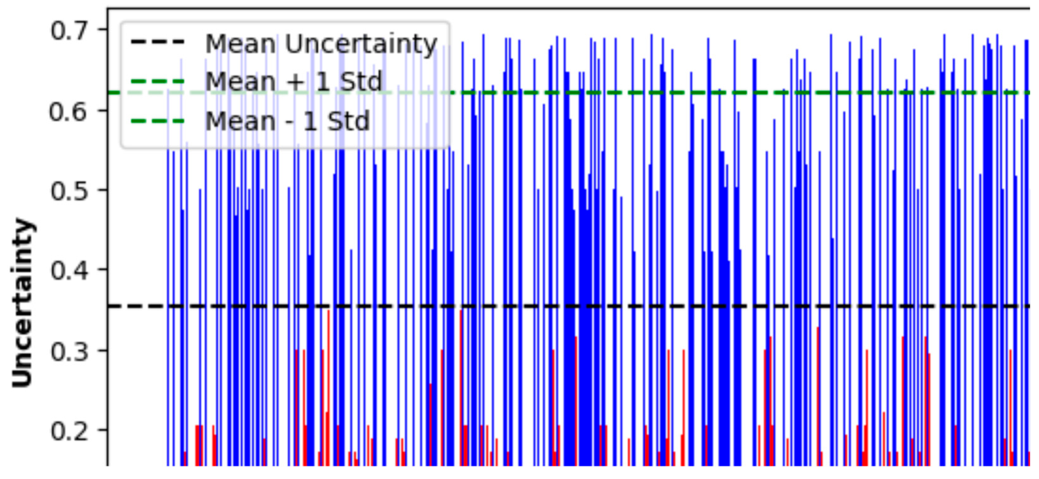
3.3. Uncertainty Analysis of EBM Model
3.4. EBM Interpretation
3.5. Limitation of the Research
- In this study, we employed different input factors extracted from the Doppler LiDAR system of HKIA to estimate the WS severity. However, it is pertinent to note that forthcoming studies may encompass additional factors, including the atmospheric pressure and temperature, that will be derived from HKIA’s weather reports.
- The main focus of the study centered on the application of EBM and other advanced ML models to forecast the severity of WS. Future research endeavors may explore the integration of additional advanced deep learning (DL) algorithms, such as wide and deep networks (WDNs) and deep and cross networks (DCNs), among others.
- The severity of WS was a notable factor of interest in this current study. The incorporation of aviation turbulence as a complementary wind attribute for future research also merits serious consideration.
4. Conclusions and Recommendation
- The performance of the EBM model differed slightly but was comparable to the XGBoost and RF models.
- The finely tuned EBM model trained on SMOTE-treated data performed better by achieving higher precision (0.98), recall (0.70), G-mean (0.77), BA (0.78), MCC (0.169), and AU-ROC values (0.854).
- The RF model trained on ADASYN-treated data demonstrated a poor performance as indicated by the precision (0.97), recall (0.53), G-mean (0.59), BA (0.59), MCC (0.105), and AU-ROC values (0.617).
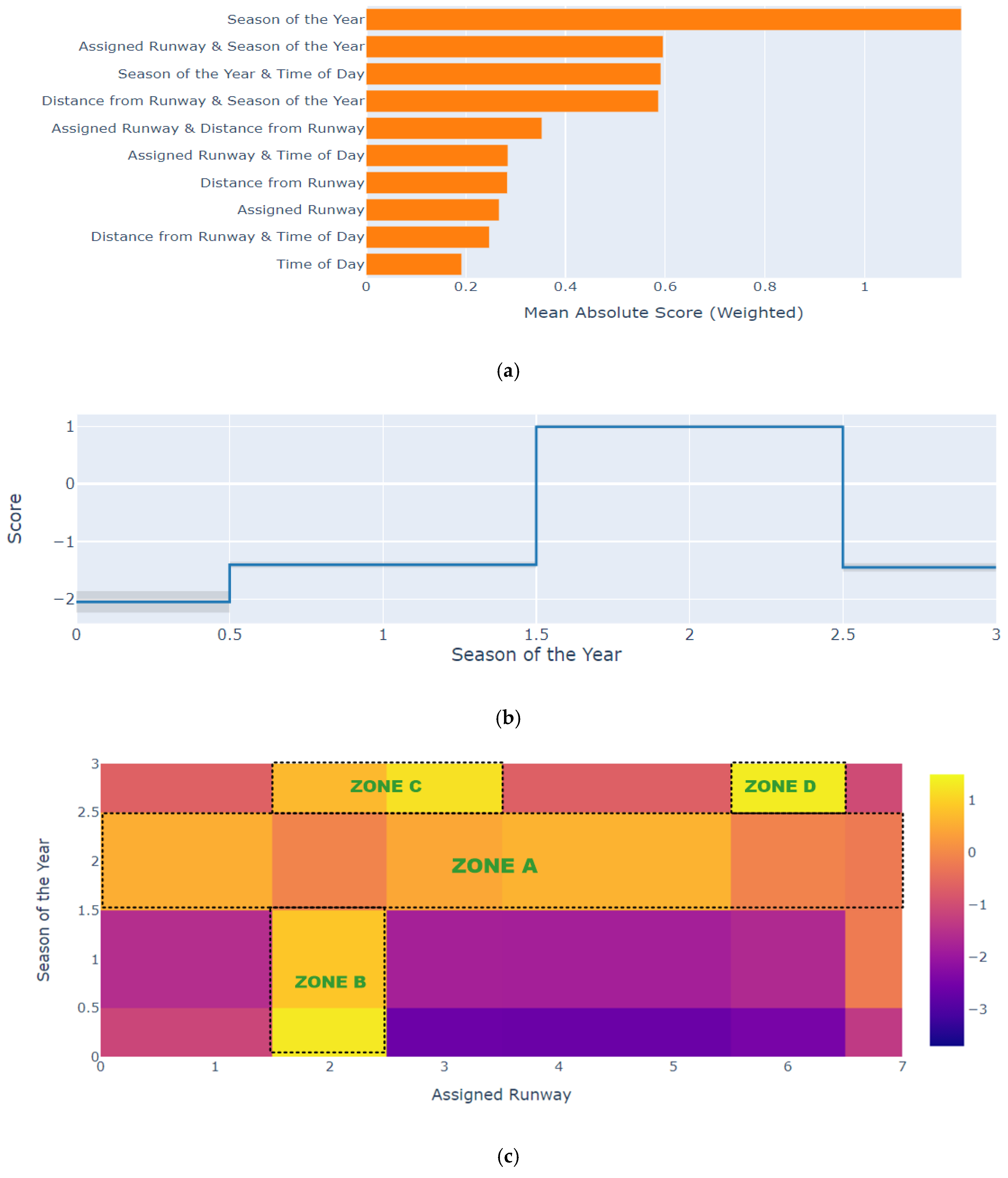
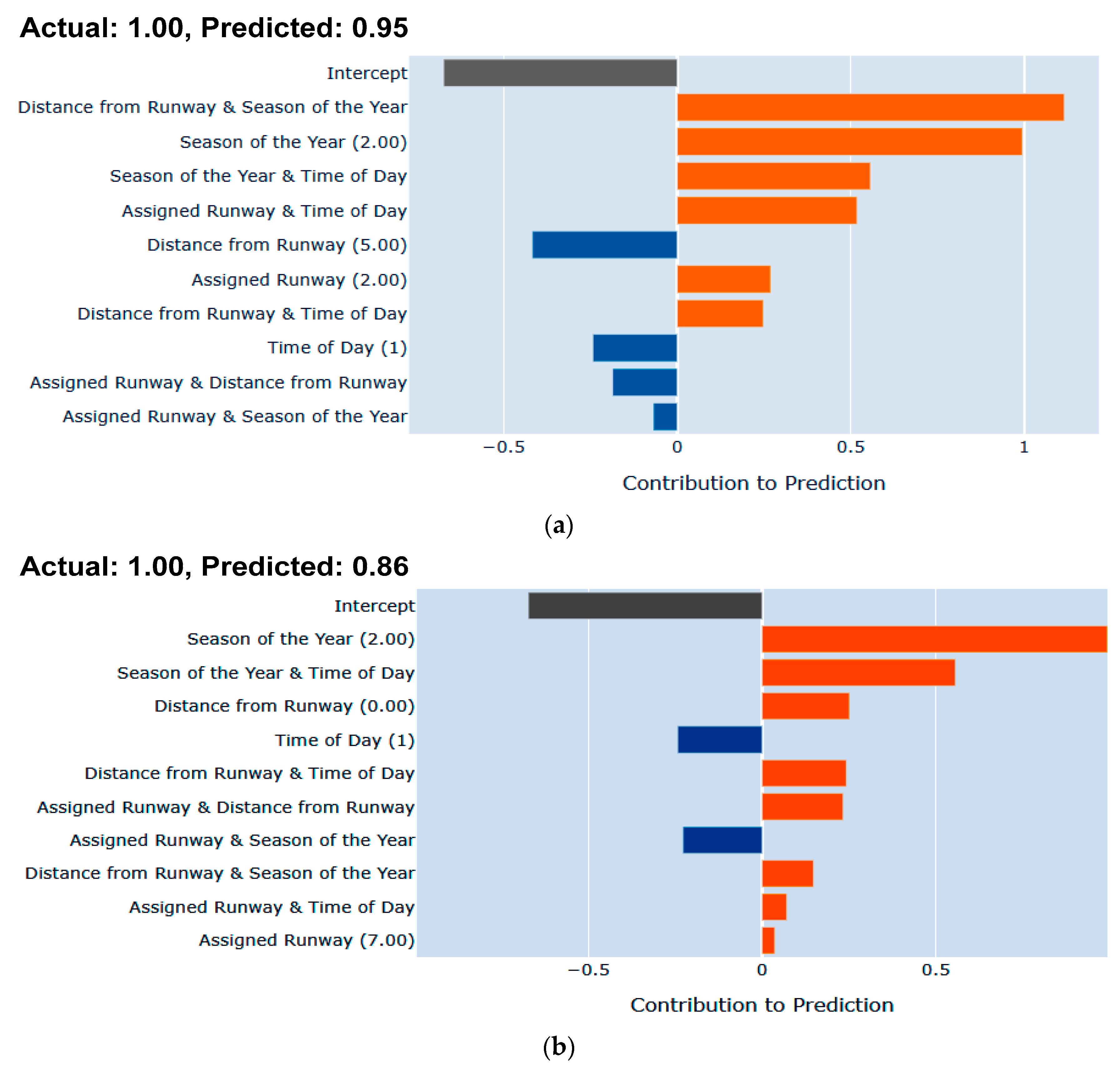
- The EBM model also showed effectiveness in the interpretation of various factors. In terms of the individual factor contribution, the season of the year contributed most to predicting the WS severity. Similarly, in terms of pairwise interaction, the season of the year and the assigned runway pair contributed most to the occurrence of SWS events.
- The interpretation via the SMOTE+EBM model revealed most of the SWS events occurred in the summer months, and all runways were prone to the occurrence of SWS. However, runway 07 RA was significantly susceptible to SWS in winter and spring, and runways 07RA, 07RD, and 25LA were susceptible to SWS events in summer.
Author Contributions
Funding
Institutional Review Board Statement
Informed Consent Statement
Data Availability Statement
Acknowledgments
Conflicts of Interest
References
- Airport Council International. World Airport Traffic Forecast 2017–2040; Airport Council International: Montreal, QC, Canada, 2017. [Google Scholar]
- Chan, P. Severe wind shear at Hong Kong International airport: Climatology and case studies. Meteorol. Appl. 2017, 24, 397–403. [Google Scholar] [CrossRef]
- Council, N.R. Low-Altitude Wind Shear and Its Hazard to Aviation; National Academies Press: Washington, DC, USA, 1983. [Google Scholar]
- Onwuadiochi, I.; Ijioma, M.; Ezenwaji, E.E.; Obikwelu, M.C. Effects of wind shear on flight operations in Sam Mbakwe Airport, Imo State, Nigeria. Trop. Built Environ. J. 2020, 7, 39–49. [Google Scholar]
- Schänzer, G.; Krüger, J. Delayed Pilot Response in Windshear. Technische Univ, Flight Simulation: Where are the Challenges? In Proceedings of the Agard Conference Proceedings 577, Braunschweig, Germany, 22–25 May 1995. [Google Scholar]
- Taszarek, M.; Kendzierski, S.; Pilguj, N. Hazardous weather affecting European airports: Climatological estimates of situations with limited visibility, thunderstorm, low-level wind shear and snowfall from ERA5. Weather Clim. Extrem. 2020, 28, 100243. [Google Scholar] [CrossRef]
- Boilley, A.; Mahfouf, J.-F. Wind shear over the Nice Côte d’Azur airport: Case studies. Nat. Hazards Earth Syst. Sci. 2013, 13, 2223–2238. [Google Scholar] [CrossRef]
- Ratnasari, Y.; Trilaksono, N.; Septiadi, D. Causes and impact of extreme Low Level Wind Shear (LLWS) event at Soekarno-Hatta International Airport. In Proceedings of the IOP Conference Series: Earth and Environmental Science, Yogyakarta, Indonesia/Online, 23–24 April 2022; p. 012011. [Google Scholar]
- Zhang, H.; Wu, S.; Wang, Q.; Liu, B.; Yin, B.; Zhai, X. Airport low-level wind shear lidar observation at Beijing Capital International Airport. Infrared Phys. Technol. 2019, 96, 113–122. [Google Scholar] [CrossRef]
- Carruthers, D.; Ellis, A.; Hunt, J.; Chan, P. Modelling of wind shear downwind of mountain ridges at Hong Kong International Airport. Meteorol. Appl. 2014, 21, 94–104. [Google Scholar] [CrossRef]
- Hon, K.-K. Predicting low-level wind shear using 200-m-resolution NWP at the Hong Kong International Airport. J. Appl. Meteorol. Climatol. 2020, 59, 193–206. [Google Scholar] [CrossRef]
- Wang, S.; De Roo, F.; Thobois, L.; Reuder, J. Characterization of terrain-induced turbulence by large-eddy simulation for air safety considerations in airport siting. Atmosphere 2022, 13, 952. [Google Scholar] [CrossRef]
- Misaka, T.; Yoshimura, R.; Obayashi, S.; Kikuchi, R. Large-Eddy Simulation of Wake Vortices at Tokyo/Haneda International Airport. J. Aircr. 2023, 60, 1819–1831. [Google Scholar] [CrossRef]
- Han, Y.; Liu, X.; Lu, X.; Li, H.; Wu, R. The 3D modeling and radar simulation of low-altitude wind shear via computational fluid dynamics method. In Proceedings of the 2016 Integrated Communications Navigation and Surveillance (ICNS), Herndon, VA, USA, 19–21 April 2016; pp. 4D3-1–4D3-9. [Google Scholar]
- Robinson, D.C.; Collins, D.; Brett, J.; Klewicki, J.; Murray, P. Airport building development: Towards a framework for managing building-induced wind shear and turbulence risks. J. Airpt. Manag. 2017, 11, 369–385. [Google Scholar]
- Laato, S.; Birkstedt, T.; Mäantymäki, M.; Minkkinen, M.; Mikkonen, T. AI governance in the system development life cycle: Insights on responsible machine learning engineering. In Proceedings of the 1st International Conference on AI Engineering: Software Engineering for AI, Pittsburgh, PA, USA, 16–24 May 2022; pp. 113–123. [Google Scholar]
- Patra, P.; Disha, B.; Kundu, P.; Das, M.; Ghosh, A. Recent advances in machine learning applications in metabolic engineering. Biotechnol. Adv. 2023, 62, 108069. [Google Scholar] [CrossRef] [PubMed]
- Thai, H.-T. Machine learning for structural engineering: A state-of-the-art review. Structures 2022, 38, 448–491. [Google Scholar] [CrossRef]
- Khawar, H.; Soomro, T.R.; Kamal, M.A. Machine learning for internet of things-based smart transportation networks. In Machine Learning for Societal Improvement, Modernization, and Progress; IGI Global: Hershey, PA, USA, 2022; pp. 112–134. [Google Scholar]
- Yuan, T.; Da Rocha Neto, W.; Rothenberg, C.E.; Obraczka, K.; Barakat, C.; Turletti, T. Machine learning for next-generation intelligent transportation systems: A survey. Trans. Emerg. Telecommun. Technol. 2022, 33, e4427. [Google Scholar] [CrossRef]
- Wang, W.; Liu, X.; Bi, J.; Liu, Y. A machine learning model to estimate ground-level ozone concentrations in California using TROPOMI data and high-resolution meteorology. Environ. Int. 2022, 158, 106917. [Google Scholar] [CrossRef] [PubMed]
- Wood, D.A. Local integrated air quality predictions from meteorology (2015 to 2020) with machine and deep learning assisted by data mining. Sustain. Anal. Model. 2022, 2, 100002. [Google Scholar] [CrossRef]
- Rudin, C. Why black box machine learning should be avoided for high-stakes decisions, in brief. Nat. Rev. Methods Primers 2022, 2, 81. [Google Scholar] [CrossRef]
- Nori, H.; Jenkins, S.; Koch, P.; Caruana, R. Interpretml: A unified framework for machine learning interpretability. arXiv 2019, arXiv:1909.09223. [Google Scholar]
- Maxwell, A.E.; Sharma, M.; Donaldson, K.A. Explainable boosting machines for slope failure spatial predictive modeling. Remote Sens. 2021, 13, 4991. [Google Scholar] [CrossRef]
- Nori, H.; Caruana, R.; Bu, Z.; Shen, J.H.; Kulkarni, J. Accuracy, interpretability, and differential privacy via explainable boosting. In Proceedings of the International Conference on Machine Learning, Virtual, 18–24 July 2021; pp. 8227–8237. [Google Scholar]
- Khattak, A.; Chan, P.-w.; Chen, F.; Peng, H. Explainable Boosting Machine for Predicting Wind Shear-Induced Aircraft Go-around based on Pilot Reports. KSCE J. Civ. Eng. 2023, 27, 4115–4129. [Google Scholar] [CrossRef]
- Konstantinov, A.V.; Utkin, L.V. Interpretable machine learning with an ensemble of gradient boosting machines. Knowl. Based Syst. 2021, 222, 106993. [Google Scholar] [CrossRef]
- Sarica, A.; Quattrone, A.; Quattrone, A. Explainable boosting machine for predicting Alzheimer’s disease from MRI hippocampal subfields. In Brain Informatics; Springer: Berlin/Heidelberg, Germany, 2021; pp. 341–350. [Google Scholar]
- Chawla, N.V.; Bowyer, K.W.; Hall, L.O.; Kegelmeyer, W.P. SMOTE: Synthetic minority over-sampling technique. J. Artif. Intell. Res. 2002, 16, 321–357. [Google Scholar] [CrossRef]
- Nguyen, H.M.; Cooper, E.W.; Kamei, K. Borderline over-sampling for imbalanced data classification. Int. J. Knowl. Eng. Soft Data Paradig. 2011, 3, 4–21. [Google Scholar] [CrossRef]
- He, H.; Bai, Y.; Garcia, E.A.; Li, S. ADASYN: Adaptive synthetic sampling approach for imbalanced learning. In Proceedings of the 2008 IEEE International Joint Conference on Neural Networks (IEEE World Congress on Computational Intelligence), Hong Kong, China, 1–8 June 2008; pp. 1322–1328. [Google Scholar]
- Wu, J.; Chen, X.-Y.; Zhang, H.; Xiong, L.-D.; Lei, H.; Deng, S.-H. Hyperparameter optimization for machine learning models based on Bayesian optimization. J. Electron. Sci. Technol. 2019, 17, 26–40. [Google Scholar]
- Chan, P.W.; Shao, A.M. Depiction of complex airflow near Hong Kong International Airport using a Doppler LIDAR with a two-dimensional wind retrieval technique. Meteorol. Z. 2007, 16, 491–504. [Google Scholar] [CrossRef]
- Chan, P. Aviation applications of the pulsed Doppler LIDAR–Experience in Hong Kong. Open Atmos. Sci. J. 2009, 3, 138–146. [Google Scholar] [CrossRef]
- Jia, B.-B.; Zhang, M.-L. Multi-dimensional classification via sparse label encoding. In Proceedings of the International Conference on Machine Learning, Virtual, 18–24 July 2021; pp. 4917–4926. [Google Scholar]
- Lou, Y.; Caruana, R.; Gehrke, J.; Hooker, G. Accurate intelligible models with pairwise interactions. In Proceedings of the 19th ACM SIGKDD International Conference on Knowledge Discovery and Data Mining, Chicago, IL, USA, 11–14 August 2013; pp. 623–631. [Google Scholar]
- Boughorbel, S.; Jarray, F.; El-Anbari, M. Optimal classifier for imbalanced data using Matthews Correlation Coefficient metric. PLoS ONE 2017, 12, e0177678. [Google Scholar] [CrossRef] [PubMed]
- Yin, J.; Gan, C.; Zhao, K.; Lin, X.; Quan, Z.; Wang, Z.-J. A novel model for imbalanced data classification. In Proceedings of the AAAI Conference on Artificial Intelligence, New York, NY, USA, 7–12 February 2020; pp. 6680–6687. [Google Scholar]
- Hon, K.K.; Chan, P.W. Historical analysis (2001–2019) of low-level wind shear at the Hong Kong International Airport. Meteorol. Appl. 2022, 29, e2063. [Google Scholar] [CrossRef]
- Chan, P.; Hon, K. Observation and numerical simulation of terrain-induced windshear at the Hong Kong International Airport in a planetary boundary layer without temperature inversions. Adv. Meteorol. 2016, 2016, 1454513. [Google Scholar] [CrossRef]
- Stocker, J.; Johnson, K.; Jackson, R.; Smith, S.; Connolly, D.; Carruthers, D.; Chan, P.-W. Hong Kong Airport Wind Shear Now-Casting System Development and Evaluation. Atmosphere 2022, 13, 2094. [Google Scholar] [CrossRef]
- Chan, P.; Lai, K.; Li, Q. Performance of large-eddy simulations for capturing low-level wind shear at the Hong Kong International Airport for a whole wind-shear (spring) season. Meteorol. Z. 2023, 32, 383–394. [Google Scholar] [CrossRef]


| WS Occurrence Date | WS Occurrence Time (Hours) | Assigned Runway | WS Horizontal Encounter Location | WS Magnitude (+/−) (Knots) |
|---|---|---|---|---|
| 12 April 2018 | 1424 | 07RA | RWY | −20 |
| 21 March 2019 | 1736 | 25RD | 1MD | +15 |
| --- | --- | --- | --- | --- |
| --- | --- | --- | --- | --- |
| 18 June 2021 | 2314 | 25LA | 1MF | −35 |
| 15 August 2022 | 0747 | 07CA | 2MF | +20 |
| --- | --- | --- | --- | --- |
| --- | --- | --- | --- | --- |
| 16 November 2022 | 2126 | 25CD | RWY | −17 |
| 21 May 2023 | 0823 | 07RA | 1MD | −25 |
| Factor | Codes and Description |
|---|---|
| Season of the year | 0: winter (December to February); 1: spring (March to May); 2: summer (June to August); 3: autumn (September to November) |
| Time of the day | 1: daytime (0700 to 1859 h); 2: night (1900 to 0659 h) |
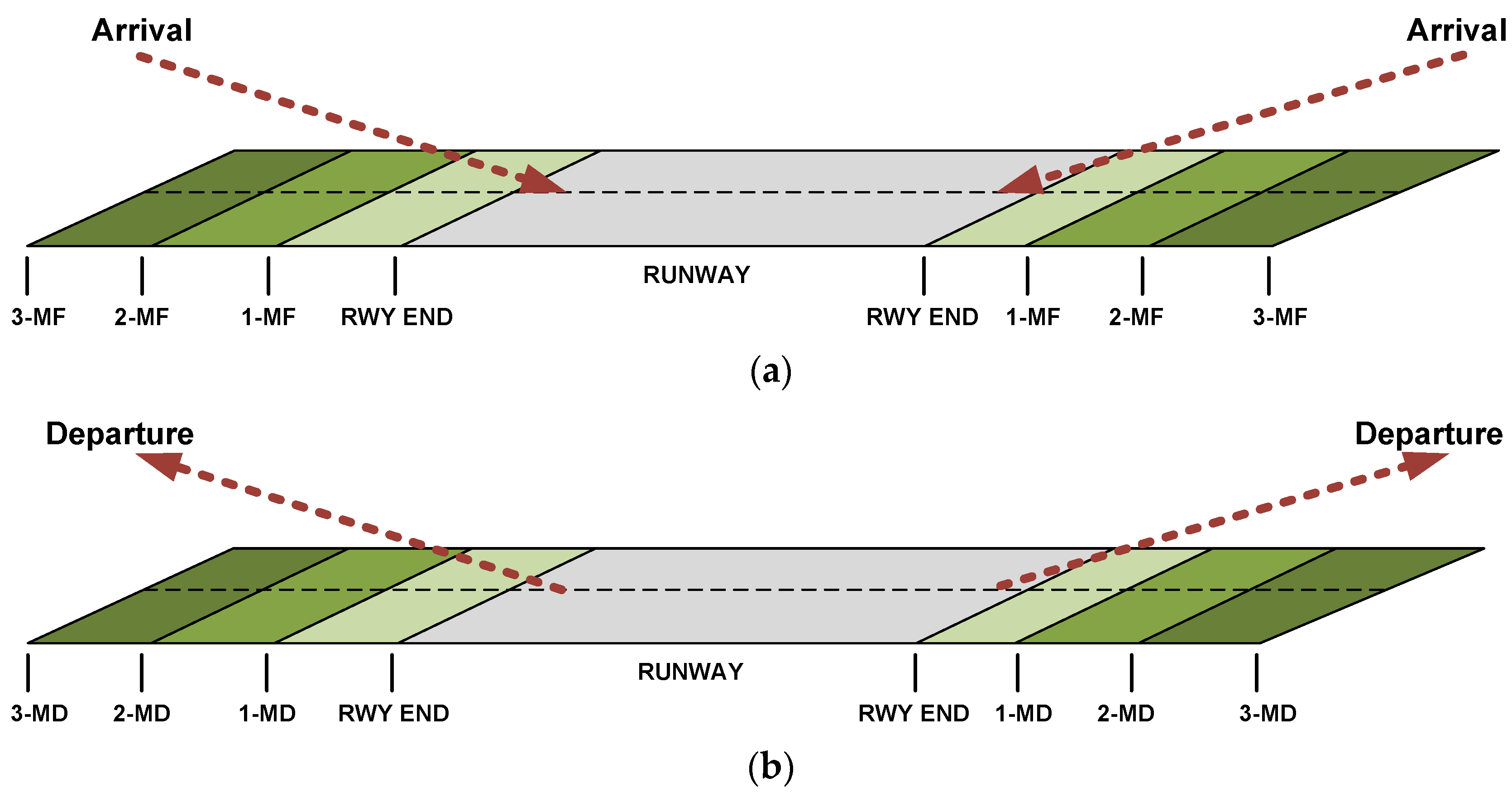
| WS encounter location | 0: RWY (occurrence of WS at runway threshold), 1: 1MF (occurrence of WS at 1 nautical miles from runway threshold at final approach); 2: 1MD (occurrence of WS at 1 nautical miles from runway threshold at departure); 3: 2MF (occurrence of WS at 2 nautical miles from runway threshold at final approach); 4: 2MD (occurrence of WS at 2 nautical miles from runway threshold at departure); 5: 3MF (occurrence of WS at 3 nautical miles from runway threshold at final approach); 6: 3MD (occurrence of WS at 3 nautical miles from runway threshold at departure) |
| Assigned runway | 0: runway 07CA; 1: runway 07CD; 2: runway 07RA; 3: runway 07RD; 4: runway 25CA; 5: runway 25CD; 6: runway 25LA; 7: runway 07LD |
| Data Treatment | Models | Optimal Hyperparameters | |||
|---|---|---|---|---|---|
| n_estimators | max_depth | learning_rate | max_leaves | ||
| SMOTE | EBM | 0.15 | 4 | ||
| DT | 3 | ||||
| RF | 670 | 4 | |||
| XGBoost | 1080 | 0.11 | 6 | ||
| SVM-SMOTE | EBM | 0.14 | 5 | ||
| DT | 3 | ||||
| RF | 730 | 5 | |||
| XGBoost | 950 | 0.07 | 6 | ||
| ADASYN | EBM | 0.16 | 5 | ||
| DT | 3 | ||||
| RF | 550 | 5 | |||
| XGBoost | 890 | 0.09 | 4 | ||
| Data Treatment | Models | True Negative (TN) | False Positive (FP) | False Negative (FN) | True Positive (TP) |
|---|---|---|---|---|---|
| SMOTE | EBM | 4410 | 22 | 1873 | 110 |
| DT | 3405 | 13 | 2882 | 119 | |
| RF | 3843 | 16 | 2444 | 116 | |
| XGBoost | 3952 | 9 | 2335 | 123 | |
| SVM-SMOTE | EBM | 4850 | 38 | 1437 | 94 |
| DT | 3405 | 13 | 2882 | 119 | |
| RF | 5159 | 59 | 1092 | 73 | |
| XGBoost | 4860 | 40 | 1427 | 92 | |
| ADASYN | EBM | 4401 | 21 | 1886 | 111 |
| DT | 3405 | 13 | 2882 | 119 | |
| RF | 3312 | 45 | 2975 | 87 | |
| XGBoost | 3915 | 11 | 2372 | 121 |
| Data Treatment | Model | Precision | Recall | G-Mean | BA | MCC |
|---|---|---|---|---|---|---|
| SMOTE | EBM | 0.98 | 0.70 | 0.77 | 0.78 | 0.169 |
| DT | 0.98 | 0.55 | 0.70 | 0.72 | 0.140 | |
| RF | 0.98 | 0.62 | 0.73 | 0.74 | 0.142 | |
| XGBoost | 0.98 | 0.63 | 0.77 | 0.77 | 0.162 | |
| SVM-SMOTE | EBM | 0.97 | 0.78 | 0.74 | 0.74 | 0.156 |
| DT | 0.98 | 0.55 | 0.70 | 0.72 | 0.140 | |
| RF | 0.97 | 0.80 | 0.68 | 0.69 | 0.139 | |
| XGBoost | 0.97 | 0.77 | 0.72 | 0.73 | 0.152 | |
| ADASYN | EBM | 0.98 | 0.80 | 0.77 | 0.77 | 0.163 |
| DT | 0.98 | 0.55 | 0.70 | 0.72 | 0.140 | |
| RF | 0.97 | 0.53 | 0.59 | 0.59 | 0.105 | |
| XGBoost | 0.98 | 0.63 | 0.75 | 0.76 | 0.157 |
Disclaimer/Publisher’s Note: The statements, opinions and data contained in all publications are solely those of the individual author(s) and contributor(s) and not of MDPI and/or the editor(s). MDPI and/or the editor(s) disclaim responsibility for any injury to people or property resulting from any ideas, methods, instructions or products referred to in the content. |
© 2023 by the authors. Licensee MDPI, Basel, Switzerland. This article is an open access article distributed under the terms and conditions of the Creative Commons Attribution (CC BY) license (https://creativecommons.org/licenses/by/4.0/).
Share and Cite
Khattak, A.; Zhang, J.; Chan, P.-W.; Chen, F.; Almujibah, H. Explainable Boosting Machine: A Contemporary Glass-Box Strategy for the Assessment of Wind Shear Severity in the Runway Vicinity Based on the Doppler Light Detection and Ranging Data. Atmosphere 2024, 15, 20. https://doi.org/10.3390/atmos15010020
Khattak A, Zhang J, Chan P-W, Chen F, Almujibah H. Explainable Boosting Machine: A Contemporary Glass-Box Strategy for the Assessment of Wind Shear Severity in the Runway Vicinity Based on the Doppler Light Detection and Ranging Data. Atmosphere. 2024; 15(1):20. https://doi.org/10.3390/atmos15010020
Chicago/Turabian StyleKhattak, Afaq, Jianping Zhang, Pak-Wai Chan, Feng Chen, and Hamad Almujibah. 2024. "Explainable Boosting Machine: A Contemporary Glass-Box Strategy for the Assessment of Wind Shear Severity in the Runway Vicinity Based on the Doppler Light Detection and Ranging Data" Atmosphere 15, no. 1: 20. https://doi.org/10.3390/atmos15010020
APA StyleKhattak, A., Zhang, J., Chan, P.-W., Chen, F., & Almujibah, H. (2024). Explainable Boosting Machine: A Contemporary Glass-Box Strategy for the Assessment of Wind Shear Severity in the Runway Vicinity Based on the Doppler Light Detection and Ranging Data. Atmosphere, 15(1), 20. https://doi.org/10.3390/atmos15010020