Abstract
In recent years, the issue of air pollution has garnered significant public attention globally, with a particular emphasis on the challenge of atmospheric fine particulate matter (PM2.5) pollution. The efficient and precise simulation of changes in pollutant concentrations, as well as their spatial and temporal distribution, is essential for effectively addressing the air pollution issue. In this paper, the WRF-Chem model is used to simulate the meteorological elements including temperature (T), relative humidity (RH), wind speed (WS), and pressure (P), and the concentrations of PM2.5 and PM10 atmospheric pollutants in December 2020 in Xuzhou City. Simultaneously, the ADMS-Urban model was employed to conduct a higher spatial resolution study of PM2.5 concentrations during the heavy pollution days of 11–12 December 2020 in Xuzhou City. The study shows that the WRF-Chem model can simulate the meteorological conditions of the study time period better, and the correlation coefficients (R) of pressure, temperature, wind speed, and relative humidity are 0.99, 0.87, 0.75, and 0.70, respectively. The WRF-Chem model can accurately simulate the PM2.5 concentration on clean days (R of 0.66), but the simulation of polluted days is not satisfactory. Therefore, the ADMS-Urban model was chosen to simulate the PM2.5 concentration on polluted days in the center of Xuzhou City. The ADMS-Urban model can simulate the distribution characteristics and concentration changes of PM2.5 around roads and buildings in the center of Xuzhou City. Comparing the simulation results of the two models, it was found that the two models have their own advantages in PM2.5 concentration simulation, and how to better couple the two models is the next research direction.
1. Introduction
In recent years, with rapid urbanization and industrialization and the continuous increase in energy consumption, air pollution has become a serious threat to public health, and its situation has gradually developed from initial urban and localized pollution to regional and compound pollution [1,2,3]. PM2.5 refers to suspended particulate matter with an aerodynamic equivalent diameter less than or equal to 2.5 µm in the atmosphere. Air pollution, especially pollution dominated by fine particulate matter PM2.5, has already caused serious impacts on atmospheric visibility, human health, regional weather, climate, etc. [4,5,6,7,8]. PM2.5 pollution has become a global problem, which has attracted special attention in several countries [9]. In recent years, as the issue of air pollution in key regions of China gained prominence, the government has implemented various pollution control and pollutant reduction measures to address the problem of atmospheric fine particulate matter pollution. Therefore, studying urban PM2.5 concentration and its pollution characteristics is of great scientific significance and research value.
The fundamental principle of numerical forecasting [10,11,12] involves numerically calculating pollutants in the atmosphere by solving the material conservation equation. Numerical forecasting is intended to simulate a real atmospheric environment, using mathematical and chemical formulas as close as possible to the real atmospheric operation mechanism, giving due consideration to the inventory of air pollution sources, meteorological factors, particle chemistry, photochemical reaction processes, secondary pollutants, pollutant transport and removal, and other factors, to simulate the calculation of the spatial and temporal distribution of pollutants. Numerical air quality prediction has undergone three generations of development in general. The first generation of air quality models is primarily characterized by Gaussian models, box models, and Lagrangian trajectory models. These models utilize wind trajectories to simulate the intricate physical and chemical processes in the near-surface atmosphere. They possess the advantage of being computationally straightforward and having relatively modest requirements for input data. In the second generation of air quality models, chemical processes were incorporated by introducing a meteorological model with a chemical reaction mechanism module. This approach gained widespread use during the 1980s and 1990s. The third generation of air quality models introduced the concept of “one atmosphere”, which fully considered the transformation and influence of complex species in the atmospheric environment, and was able to solve a variety of complex atmospheric problems.
The WRF-Chem model, as a third-generation air quality model, is a newly developed regional atmospheric dynamics–chemistry coupled model in the U.S. It is integrated by adding an atmospheric chemistry module to the Weather Research and Forecasting Model (WRF) developed by NCAR, and it has been widely used for atmospheric pollutant simulation and numerical forecasting. Shukla et al. [13] examined the dust storm that transpired across the northwest Indo-Gangetic Plain in June 2018 utilizing the WRF-Chem model. Their findings indicated that the model effectively replicated both the horizontal and vertical distributions of dust aerosols in alignment with observations. However, the model’s estimated concentrations of sand and dust aerosols were marginally lower compared to the Modis AOD’s results. Qiao et al. [14] conducted a comparison of air pollutant concentrations over Guangzhou City using simulations from the WRF-Chem model against those from the back propagation neural network (BPNN) model and the long short-term memory (LSTM) model. The results indicated that WRF-Chem exhibited superior performance in simulating gaseous pollutant concentrations. However, it did not match the performance of the other two models in simulating particulate matter concentrations. Shahid et al. [15] simulated the seasonal spatial and temporal variations of aerosols, tropospheric ozone, and dust over the Middle East (ME) in 2012 using the WRF-Chem model, and achieved better simulation results. Do et al. [16] used the WRF-Chem model to simulate the meteorological variables in winter and summer in northern Vietnam in 2014, along with the local PM2.5 and PM10 concentrations, and showed that although the simulation results had a good spatial and temporal consistency with observations, the amount of day-to-day variability at each observation site was difficult to capture, which may be related to either the model itself or the input emissions data. Dorita et al. [17] employed a combination of the WRF-Chem and RTFDDA models to forecast dust storms in the Middle East and northern Africa, aiming to analyze the horizontal and vertical distribution of dust. The study demonstrated that the model effectively replicated the primary characteristics of the investigated dust storms. Georgiou et al. [18] used the WRF-Chem model for daily 3D forecasts of regulated pollutants such as NO2, O3, and PM2.5 over the eastern Mediterranean Sea, and compared the simulation results with predictions from the European Union Copernicus Atmospheric Monitoring Service (CAMS). The predictions of surface temperature, pressure, and wind speed were found to be accurate, with minor differences in the 10 m wind speeds. The WRF-Chem model accurately simulated NO2 and O3 concentrations, but overestimated PM2.5 concentrations affected by long-range transport in winter.
The ADMS-Urban model, as a new generation of steady-state atmospheric dispersion model, is suitable for simulation from street scale to large city scale, and is widely used for air quality evaluation and prediction under complex conditions in towns, cities, highways, and large industrial bases, etc. Owen et al. [19] utilized urban emission inventory data alongside the ADMS-Urban model to simulate NOx concentrations within the city of London, synthesizing the performance of the modeling system in order to predict the concentrations of emission sources in London. The study achieved a robust validation by comparing the simulated results with observed data. He et al. [20] integrated the ADMS-Urban model with the land use regression (LUR) model to investigate the simulation of NO2 concentrations in Guangzhou City. The study demonstrated improved accuracy when compared to the concentration values observed at monitoring stations. The combined model was applied to the simulation of NO2 concentration in other cities. Munir et al. [21] utilized the ADMS-Urban model, integrating information on pollutant emissions from road vehicles and meteorological parameters, to simulate atmospheric PM10 and PM2.5 concentrations in Makkah City. The resulting values were compared with measurements from local observatory sites. The study concluded that the ADMS-Urban model underestimated the PM concentrations, suggesting the potential need for more precise and extensive emission data to enhance the model’s performance. Dimitrova et al. [22] employed the ADMS-Urban model to simulate the PM concentration levels in the Sofia region during winter. The study aimed to investigate the impact of four major emission sources (point industries, residential heating, roadways, and unorganized transportation) on air pollution and quality of life in the city of Sofia by controlling variables. Michael et al. [23] utilized the ADMS-Urban model and a detailed road emission network to simulate street-scale variations in nitrogen oxides, NO2, and PM2.5 concentrations during the winter of 2016 in major Chinese cities. The study indicated an overestimation of NO2 concentrations near roadways, while PM2.5 concentrations were underestimated. This discrepancy might be due to insufficient PM2.5 emissions and spatial variability.
It can be seen that the WRF-Chem model and the ADMS-Urban model have been widely used in simulating the concentration of atmospheric pollutants [24,25,26,27], and the WRF-Chem model, as a third-generation air quality model at the regional scale, introduces a more complex chemical mechanism while taking into account the feedback effect of pollutants, such as aerosols, on the meteorological field, and is able to simulate the concentration of atmospheric pollutants more accurately. The WRF-Chem model offers the capability of regional nesting, allowing for the study of pollutant distribution and characteristics on a broader scale. The model allows for an unlimited number of nested layers, enabling the implementation of multi-layer nesting, typically with 3–5 layers. The simulation of air pollutants can be realized from the perimeter of the study area to the local area with higher spatial resolution. However, the current maximum spatial resolution of the innermost nested simulation of WRF-Chem is 1 km, which does not allow for studies of pollutant concentrations at a higher spatial resolution. The WRF-Chem simulations exhibit a relatively good fit to the observations, showing strong agreement in simulating peak concentrations. However, on days with high pollution levels, the simulated values of air pollutants tend to be underestimated. Therefore, higher precision models are needed for more refined studies. The ADMS-Urban model, as a new generation of urban-scale air quality model, can simulate the distribution of pollutant concentrations in and around urban centers more concisely, quickly, and in detail. This enables the simulation of atmospheric pollutant concentrations at a higher spatial resolution. The ADMS-Urban modeling benefits from the input of increasingly accurate emission source data, leading to simulated values that closely align with observed values. Nevertheless, obtaining more emission data specifically from road sources, as required with ADMS-Urban, can pose challenges. In some cases, there may be difficulties in obtaining a comprehensive set of road emission data, resulting in instances of missing information. If a broader range of air pollutant concentration values is being modeled, it may be necessary to invest significant human resources in the actual measurement of road data information. This limitation restricts the model to smaller, more accurate simulations. The ADMS-Urban model requires a considerable amount of time to run, and as the size of the study area increases, the duration for running the model also extends. However, ADMS-Urban simulations can attain an impressive spatial resolution at the “meter” level that is challenging for other atmospheric chemistry models to match. As the model evolved, the ADMS-Urban RML model gradually began to be used. The model links the ADMS-Urban regional model to provide high-resolution modeling that enables automatic coupling with the regional meteorological model (WRF) and air quality models (CMAQ, CAMx, CHIMERE, EMEP4UK, and WRF-Chem). However, the model has been less frequently utilized by researchers for conducting studies, and its simulation effectiveness remains unassessed at present. Nevertheless, it can serve as a noteworthy point to illustrate the potential feasibility of coupling the two models for studying air pollutant concentrations. Therefore, the study of air pollutant concentrations by coupling the two models simultaneously can better simulate the spatial and temporal changes and spatial distribution of air pollutant concentrations in the study area.
Existing air quality studies can be categorized into global-scale modeling and regional-scale modeling. The GEOS-Chem model, widely employed by scholars, operates as a global-scale atmospheric chemistry model. However, there are fewer studies focused on urban-scale air quality using this model. The WRF-Chem model is widely used in the simulation of atmospheric pollutants at the regional scale, but the spatial resolution of the model simulation is limited. Therefore, this paper proposes the approach of using the WRF-Chem model to simulate pollutant concentrations for all time periods and using the ADMS-Urban model to refine the study for days where there are large deviations in the simulation of pollutant concentrations. In this paper, we employ the WRF-Chem model to simulate meteorological factors, including wind speed, temperature, and humidity, as well as PM2.5 and PM10 concentrations in Xuzhou City for December 2020. These simulated values are then compared with observations from monitoring stations. The modeling results revealed a greater bias in PM2.5 pollutant concentrations on more polluted days. Consequently, for further investigation, two days characterized by heavy pollution on 11–12 December were selected for refinement using the ADMS-Urban model to enhance the accuracy of pollutant concentrations in Xuzhou City on these specific days. This offers a rapid and precise detection method for identifying increased pollutants in localized city areas, serving as an effective approach for monitoring urban air quality and implementing pollution control measures as needed.
2. Data and Methods
2.1. Study Area
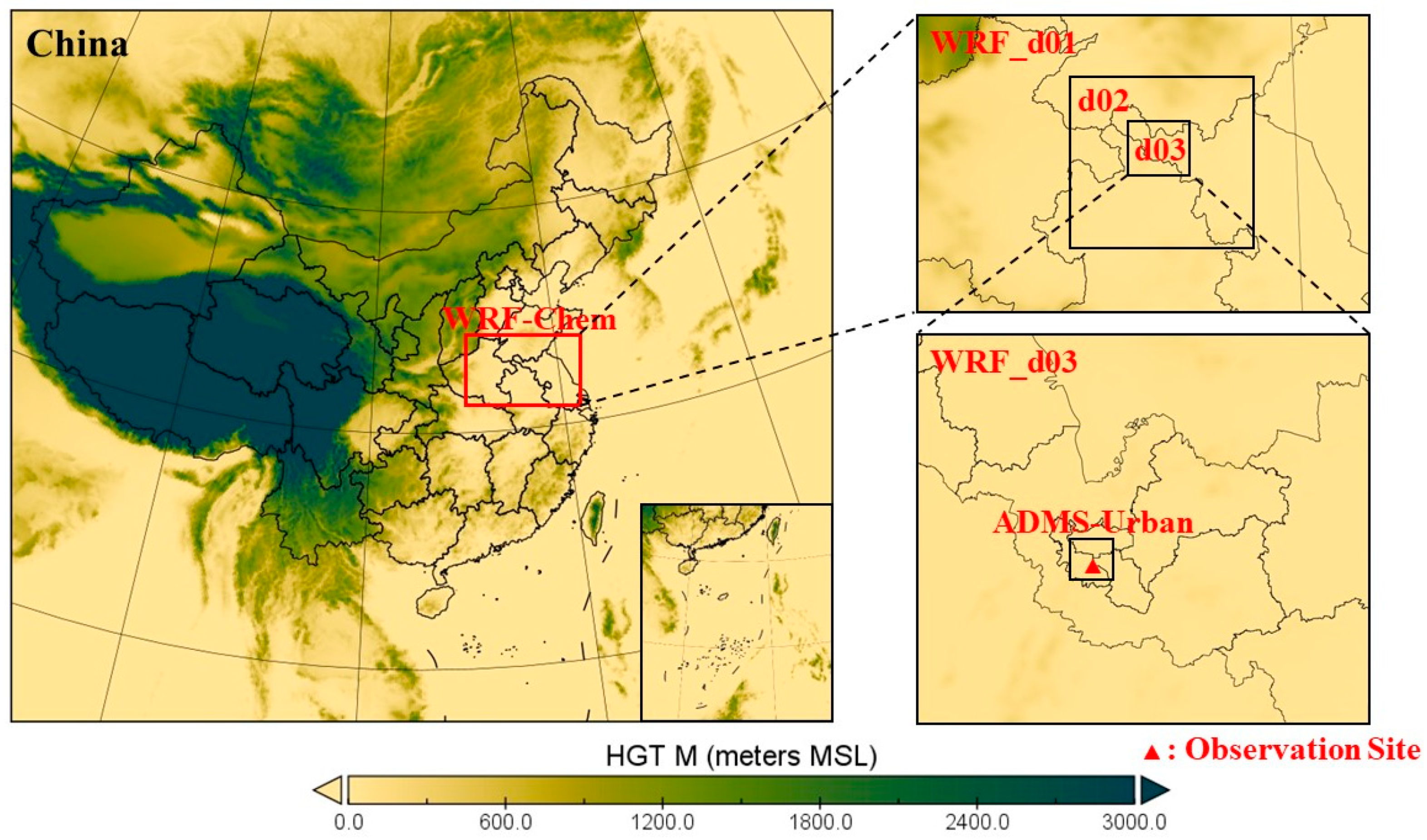
Xuzhou is a prefecture-level city in Jiangsu Province, China, located in the northwestern part of East China, connecting North and East China as well as the central and western regions. It is an important city at the junction of four provinces in China, and an important transportation hub on the Beijing–Shanghai Railway. In recent years, Xuzhou, being a heavily industrialized city, has faced severe air quality issues [28,29,30,31]. Consequently, the government has consistently intensified air pollution control measures and expedited energy restructuring efforts to ameliorate the air quality situation. The Xuzhou Environmental Quality Bulletin shows that the number of days in 2020 when the ambient air quality in Xuzhou urban area reached Grade 2 or above was 261 days, an increase of 45 days compared with 2019, and the good rate of ambient air quality in Xuzhou urban area in 2020 was 71.3%, an increase of 12.1 percentage points compared with 2019, but the concentration of major air pollutants is still at the level of higher values. Therefore, it is typical and representative to choose Xuzhou as the study area of this paper. Analyzing the spatial and temporal distribution of air pollutants in Xuzhou is of great significance for studying the air pollution situation in the region, and also provides reliable data support for subsequent air governance and management. As of 2020, Xuzhou City is equipped with seven monitoring stations. For the validation of air pollutant concentrations in this paper, actual observations were sourced from the Huaita observation site (Figure 1), situated at latitude and longitude coordinates of 117°11′30″ E, 34°13′58″ N.
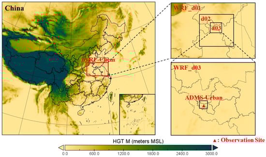
Figure 1.
Study area setup for WRF-Chem and ADMS-Urban models. The colors in the figure are the terrain heights in the WRF.
2.2. WRF-Chem Model
WRF (the Weather Research and Forecasting Model) is a new generation of mesoscale numerical simulation and data assimilation system. It encompasses multiple dynamical cores, a three-dimensional variational (3DVAR) data assimilation system, and a software architecture designed to accommodate parallel computation and system scaling [28]. The atmospheric chemistry model WRF-Chem used in this paper couples all the transport processes of the chemical transport module Chem and the meteorological model WRF [29]. The meteorological module and chemical module utilize identical vertical and horizontal coordinates, sharing the same physical parameterization scheme, allowing for the consideration of the feedback effect of chemistry on meteorological processes. Therefore, the WRF-Chem model can, on the one hand, be used to predict and simulate weather conditions, including physical quantities such as temperature field, wind field, boundary layer, and cloud and rain processes with the full functionality of the WRF model and, on the other hand, it can also be used to couple weather forecasting and atmospheric dispersion modeling to simulate the components of emissions and transport, and to simulate the interactions of gaseous pollutants and substances such as PM particles, and so on.
The WRF-Chem model is divided into three main modules, including the WPS data preprocessing module, the WRF-AWR master integration module, and the post-processing module. In this study, we used WRF-Chem version 3.6.1, and the model needs to be run under Linux environment. The WRF model incorporates various physical parameterization schemes, encompassing a range of physical processes. These include horizontal and vertical vorticity dispersion, short-wave and long-wave radiation schemes, microphysical process schemes, cumulus parameterization schemes, boundary layer schemes, urban canopy schemes, land surface process schemes, and others. A gas-phase chemistry mechanism is an important component in regional air pollution modeling, and WRF-Chem provides several optional gas-phase chemistry mechanisms; commonly used ones are RADM2 (Regional Acid Deposition Model version 2) [30], RACM (Regional Atmospheric Chemistry Mechanism) [31], CBMZ (Carbon-Bond Mechanism version Z) [32], CB- 4 (Carbon Bond 4) [33], CB05 (Carbon Bond 2005) [34], SAPRC99 (the 1999 version of the Statewide Air Pollution Research Center Mechanism) [35], and so on. For aerosol chemistry mechanisms, the WRF model provides five available schemes, namely the MADE/SORGAM (Modal Aerosol Dynamics Model for Europe) scheme [36,37], the MADE/VBS (Modal Aerosol Dynamics Model for Europe with the Volatility Basis Set for aerosols) scheme [38], MAM (Modal Aerosol Module) 3bins and 7bins schemes [39], MOSAIC (Model for Simulating Aerosol Interactions and Chemistry) 4bins and 8bins programs [40], and the GOCART box aerosol program [41].
In this study, the investigation focused on atmospheric PM2.5 pollution in Xuzhou City for December 2020. The model was configured with three nested layers, featuring outermost spatial resolutions of 9 km × 9 km, followed by 3 km × 3 km, and 1 km × 1 km. The innermost region encompasses the entirety of Xuzhou City, serving as the study area for this experiment, as depicted in Figure 1. After debugging with different experimental sensitivities, the experiment finally chose a set of parameters that can better simulate the atmosphere for the experiment. The specific set of physical and chemical parameters are shown in Table 1.

Table 1.
Model scheme and parameter settings.
Input data for the model include meteorological reanalysis data, initial and boundary field data, and emission inventory data, including biological and anthropogenic emission sources. The meteorological reanalysis data used in the article were provided by the U.S. National Centers for Environmental Prediction (NCEP) FNL Global Operational Analysis data [50], with a horizontal grid resolution of 1° × 1°, and a spatial resolution of 6h at 00:00, 06:00, 12:00, and 18:00 (UTC). The chemical boundary field chosen in this paper is CAM-Chem [51], primarily designed for modeling atmospheric components in the global troposphere and stratosphere. The chemistry in CAM-Chem is primarily based on the MOZART family of chemical mechanisms, which contains a wide range of different chemical options. The biogenic emissions utilized in this paper originate from MEGAN (Model of Emissions of Gases and Aerosols from Nature) data [52]. An online tool was employed to process the global biogenic emissions dataset, which maintains a spatial resolution of 1 km × 1 km, and transform it into gridded data that aligns with the spatial extent of the modeled region. The inventory of anthropogenic emission sources used in this paper is the Multi-Resolution Emission Inventory Model for Climate and air pollution research (MEIC) from Tsinghua University [53,54], which is a set of cloud-based inventory of China’s anthropogenic emissions of air pollutants and greenhouse gases, including the industrial, power plant, residential, transportation, and agricultural emissions of five major categories of anthropogenic sources. The version of the data used in this study is MEIC v1.4.
2.3. ADMS-Urban Model
The ADMS-Urban model, as a new generation of steady-state atmospheric dispersion model, applies the latest atmospheric boundary layer and atmospheric dispersion theories to the air pollutant dispersion model by applying the latest available atmospheric physical theories based on the parameters of the Monin–Obukhov length and boundary layer height describing the structure of the boundary layer [55,56]. ADMS-Urban builds upon ADMS-EIA’s capability to handle increased volumes of contaminants and conduct more intricate chemical reaction simulations. The ADMS-Urban model specializes in modeling air quality in extensive urban areas, towns, and cities, achieving a remarkably high spatial resolution that extends to the “meter” level [57]. The ADMS-Urban model has the capability to account for highly intricate urban configurations, encompassing streets, mountain ranges, canyons, and more. It can provide simulations of short- and long-term average pollutant concentrations ranging from the street scale up to the city scale. As a result, the input data for the ADMS-Urban model includes on-road emission source data and meteorological data with higher accuracy. In the ADMS-Urban model, the boundary layer structure can be defined using conventional meteorological elements, thus better describing the atmospheric dispersion process and making the prediction of pollutant concentrations more accurate and credible. The model’s input data encompass meteorological data, digital map data, and emission data originating from pollution source areas. This includes point source emission data (such as smokestacks and industrial organized sources), line source emission data (road emission data), and surface source emission data (including material yards, construction sites, etc., and industrial unorganized sources). The land use classification data used in this study were obtained using visual interpretation and supervised classification processing of Gaofen-1 remote sensing images. Traffic flow data is obtained by manually counting the vehicle information of typical roads combined with the interpolation of real-time traffic congestion data of roads released by Gaode Map. The wind farm data and meteorological data were obtained from the Xuzhou Air Quality Gridded Monitoring website.
The simulation range set up in this study is a small part of the city center, including the Quanshan District, Gulou District, and Tongshan District of Xuzhou City, and the specific study area is shown in Figure 1. 11–12 December 2020 were selected as the study dates, and the ADMS-Urban model was used to simulate the PM2.5 concentrations in the center of Xuzhou City on those two heavily polluted days.
2.4. AQI Calculation
The AQI (Air Quality Index) [58,59] is a dimensionless index that quantitatively describes air quality conditions. In calculating the AQI, the Individual Air Quality Index (IAQI) for a total of six items of each of the participating factors (fine particulate matter (PM2.5), respirable particulate matter (PM10), sulphur dioxide (SO2), nitrogen dioxide (NO2), ozone (O2), and carbon monoxide (CO)) is calculated first, and the maximum value of the IAQI for each of the participating factors is taken as the value of the AQI. The AQI operates on the principle that a higher value indicates a higher level and category of air pollution, reflecting a more severe air pollution condition [60,61]. When the AQI exceeds 50, the air pollutant with the largest IAQI becomes the primary pollutant.
The IAQI for Pollution Project P is calculated as follows:
where IAQIp is the IAQI of pollutant item P; Cp is the value of the quality concentration of the pollutant item P; BPHi is the high value of the pollutant concentration limits similar to C in Table 2; BPLi is the lower value of the pollutant concentration limits similar to C in Table 2; IAQIHi is the IAQI corresponding to BPHi in Table 2; and IAQILo is the IAQI corresponding to BPLo in Table 2. The IAQI is calculated as follows:
where n is the pollutant program. The IAQI and the corresponding concentration limits of pollutant items are shown in Table 2.
Table 2.
Individual Air Quality Index and the corresponding concentration limits of pollutant items.
2.5. Model Validation and Evaluation
The station monitoring data utilized in this study were provided by the China National Environmental Monitoring Centre (CNEMC). These data consist of hourly concentrations of six major pollutants, including PM2.5 and PM10. Specifically, the PM2.5 concentration in Xuzhou City was employed for comparison and validation against the simulation values generated with the WRF-Chem model. The hour-by-hour meteorological observations data used in the study were provided by the China Meteorological Data Service Centre, in which the monitored values of temperature, wind speed, and relative humidity in Xuzhou were used for comparison and validation with the simulated values of the WRF model. We examined the simulation effects of meteorological elements and pollutant concentrations, respectively. The statistics we used for the comparative analysis of station data were the mean bias (MB), normalized mean bias (NMB), normalized mean gross error (NME), root mean square error (RMSE), and correlation coefficient (R). The mathematical expressions for the four indicators are as follows:
where Cm is the simulated value, Co is the observed value, and n is the number of samples. NME and NMB are dimensionless quantities, the former describes the average degree of deviation between simulation and observation, the latter describes the degree of deviation between simulation and observation, and RMSE reflects the average error between simulated and observed values.
3. Results and Discussion
3.1. Simulation of PM Concentration
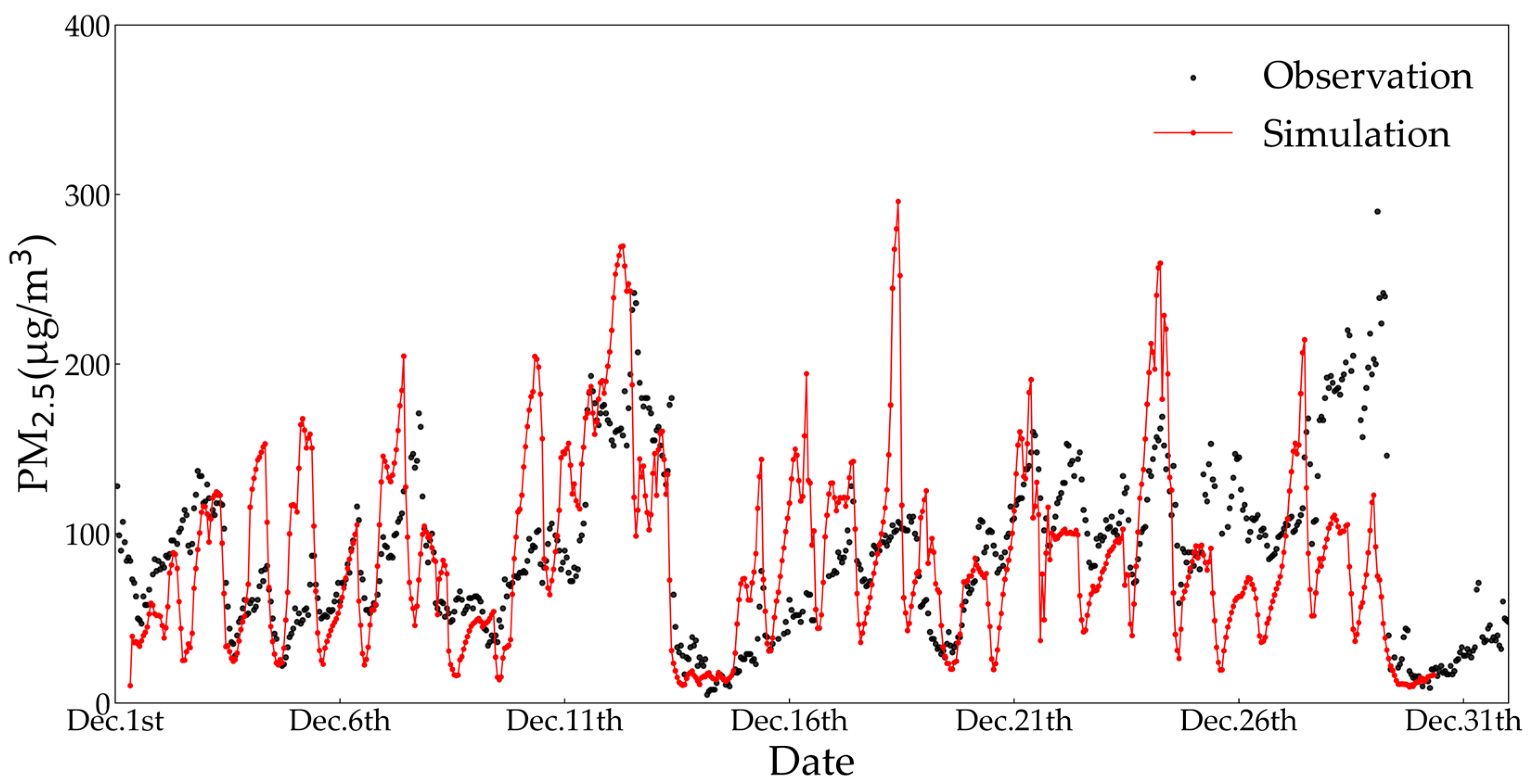
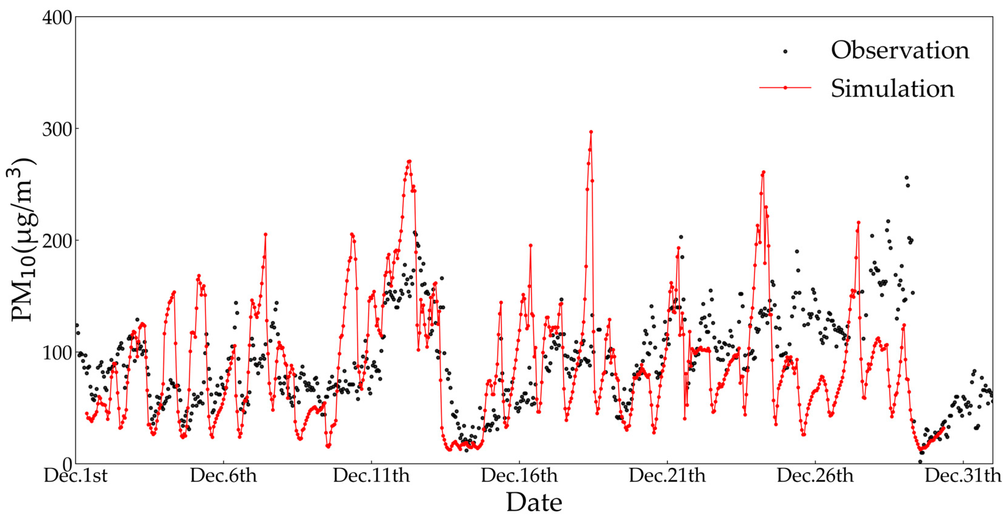
The simulation of PM2.5 concentration with the WRF-Chem model is shown in Figure 2, and it can be seen that the model well simulates the trend of daily average PM2.5 change in this month, with a correlation coefficient of 0.63. The model can simulate the trend of concentration growth and abatement during heavy pollution events, but there is an issue with the simulated peak concentration of PM2.5 differing significantly from the actual observed concentration. For example, PM2.5 concentrations increased on 17–18 December compared to 15–16 December. The observed PM2.5 concentrations ranged from about 80 μg/m3 to 100 μg/m3, with the maximum observed PM2.5 concentration being 110 μg/m3. The model simulation indicated an increase in PM2.5 concentration for these two days, with simulated values ranging from approximately 80 μg/m3 to 250 μg/m3. However, the extreme simulated value was excessively high, reaching a maximum value of 295 μg/m3. After conducting research and analysis, it appears that there might have been a slight decreasing trend in actual PM2.5 concentrations. This could be attributed to the abrupt decrease in weather temperatures, coupled with an increase in the number of foggy days during the study period. However, the model was unable to simulate this temporal change. The observed PM2.5 concentrations on the two days of 28–29 December were 180–200 μg/m3, while the simulated values of PM2.5 concentrations ranged from 80–100 μg/m3, again indicating that the model’s simulation of the pollutant is sometimes subject to large deviations. There are two potential factors contributing to the discrepancies observed. Firstly, the modeled pollutant concentrations may lack accuracy due to significant uncertainties in the local emission inventories. Secondly, the model might struggle to conduct a more precise analysis of pollutant dispersion and flow effects. This could be attributed to a slight bias in simulating meteorological conditions, such as wind speed. This prevents local PM2.5 pollutant concentration deposition or dispersion from being well modeled, and as air masses bring in concentrations of exotic atmospheric pollutants, the simulation can be similarly affected, making the model less accurate in simulating pollutants. The WRF-Chem model’s simulation of PM10 concentration is depicted in Figure 3. Upon comparing the simulation outcomes with the measured results at the site, it is evident that the model performs better in simulating PM10 concentration. Comparing Figure 2 and Figure 3, the model simulations of PM2.5 and PM10 are roughly similar, indicating that the primary atmospheric particulate matter in Xuzhou City is PM2.5. To further evaluate the effectiveness of the experiment on model simulation of PM2.5 concentrations, the study time period was divided into polluted days (11–12 December and 27–28 December) and clean days (excluded polluted days for the whole month of December) and different metrics were calculated for all days of the whole month, clean days, and polluted days, respectively (Table 3). It can be seen that the WRF-Chem model simulates the PM2.5 concentration on clean days more closely, with a smaller resultant bias and root mean square error. The results are better than the simulation evaluation of all days in the whole month, which indicates that the model is more accurate in simulating PM2.5 concentration on clean days. In contrast, the simulated values of PM2.5 concentration with the WRF-Chem model on heavily polluted days resulted in large bias and root mean square errors, indicating that the model has poor accuracy in simulating air pollutants on heavily polluted days.
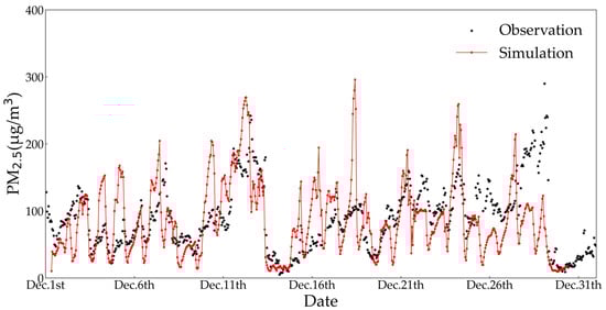
Figure 2.
Comparison of simulations and observations of PM2.5 concentrations in Xuzhou in December 2020.
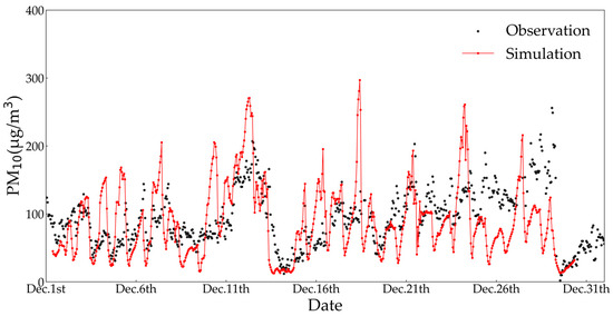
Figure 3.
Comparison of simulations and observations of PM10 concentrations in Xuzhou in December 2020.
Table 3.
Statistics of simulations and observations of PM2.5 and PM10 concentrations in Xuzhou in December 2020.
3.2. Simulation of Meteorology
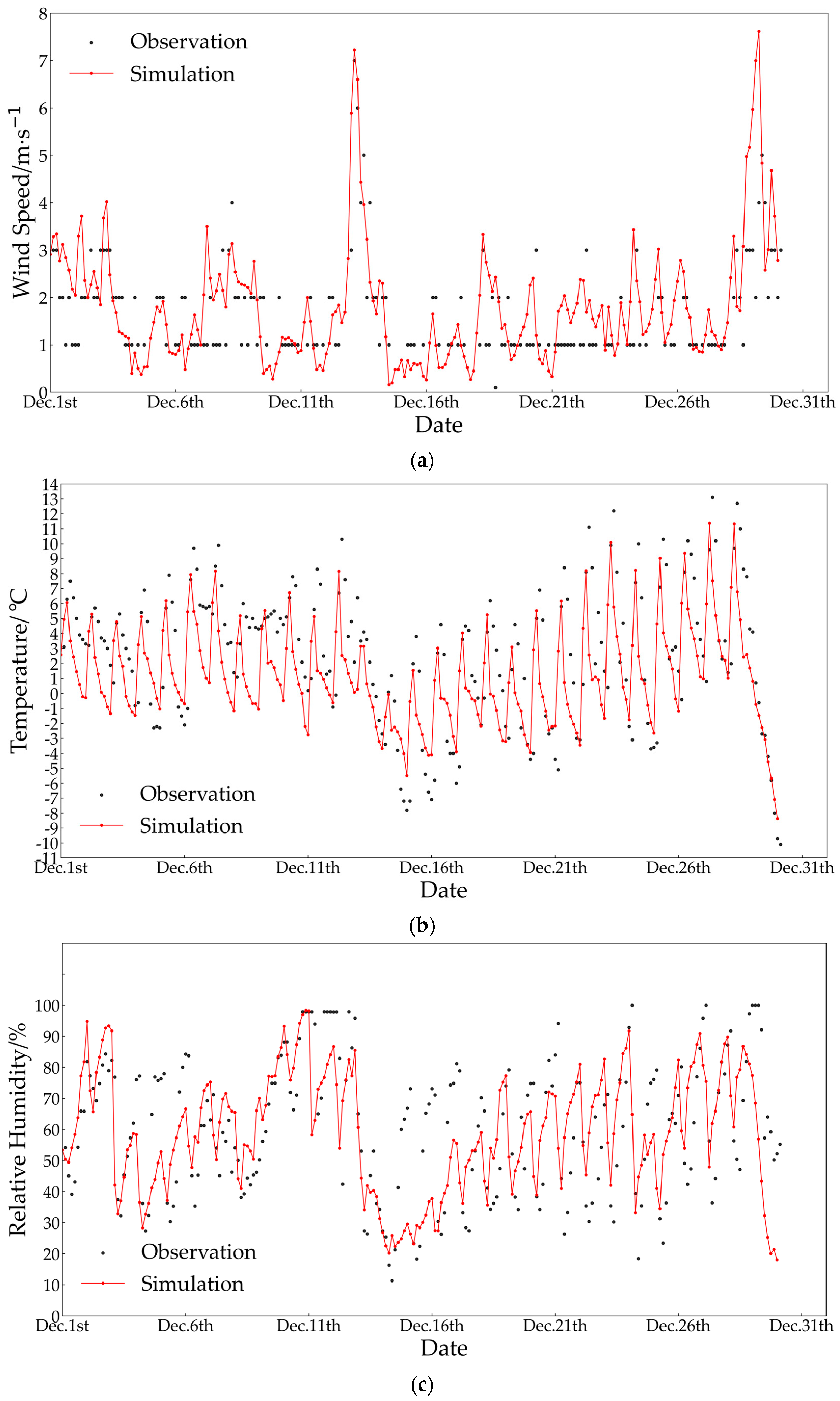
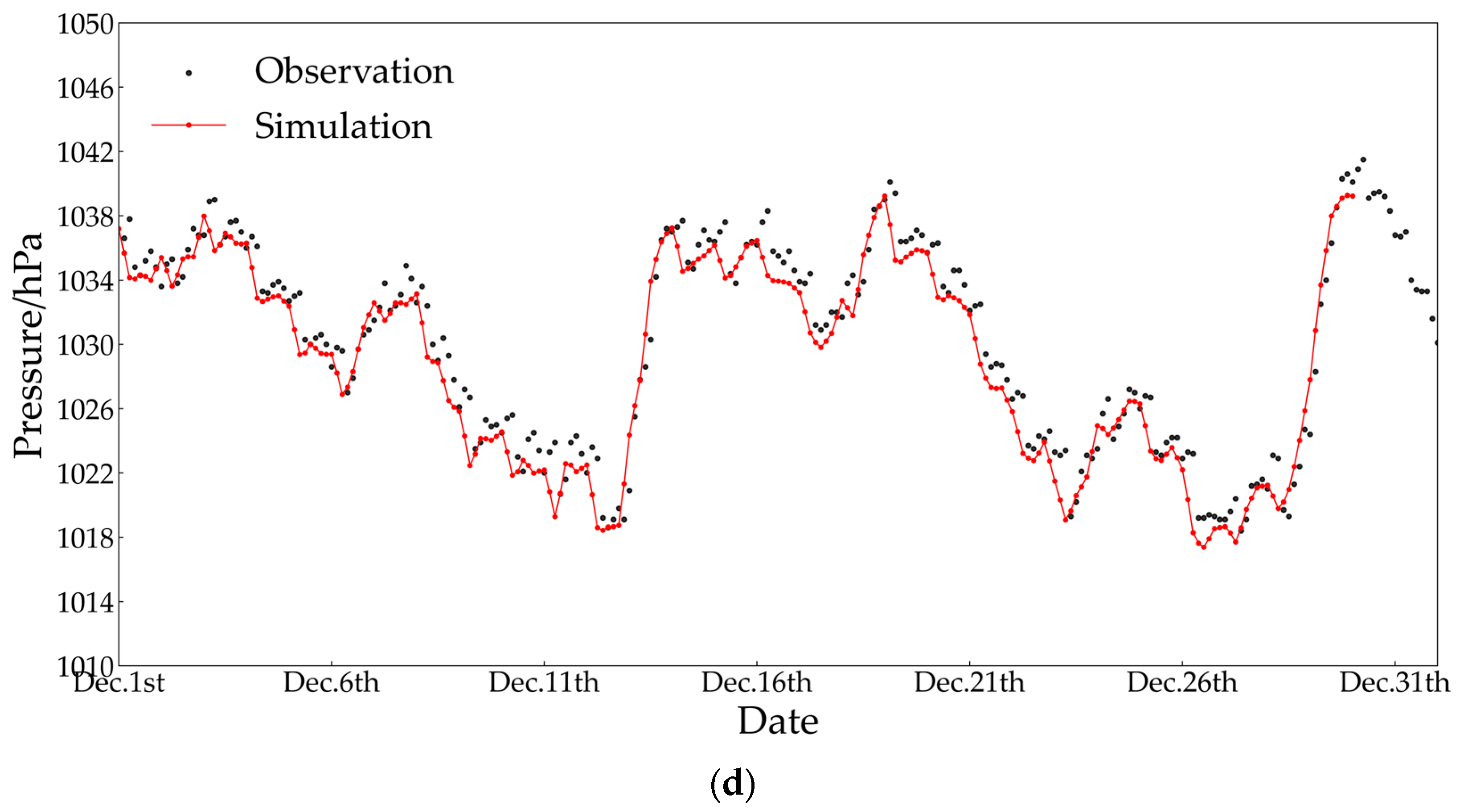
In this study, WRF was used to simulate the main meteorological parameters of Xuzhou City in December 2020, and the observations were selected for comparison and validation with the simulation results, including the variables of temperature (T), relative humidity (RH), wind speed (WS), and pressure (P). The simulations of meteorology for every three hours were compared with the observations (Figure 4), where (a)–(d) are the simulation results of WS, T, RH, and P for the month, respectively, and the black and red dots in the line graph represent the meteorological observations and the simulations of WRF, respectively. As visualized in the figure, the meteorological parameters are simulated better, and the results of both the extreme value and trend simulations are in good agreement with the observations at the station. The results of the evaluation of the model are shown in Table 4, with R values of 0.99, 0.87, 0.75, and 0.70 for P, T, WS, and RH, respectively. The simulations exhibit a high correlation with observations for P, T, and WS, while the correlation for RH is moderate. The stability of the simulation results is generally favorable, with simulated data exhibiting minimal deviation from observed data. However, there are still some periods during which substantial errors are observed. For example, there is a significant overestimation of the minimum value of T on 15–17 December, as well as a very serious underestimation of the extreme values of RH on 3–5 December and 16–18 December. There is a general underestimation of P simulated with WRF, but the NMB and NME values are almost zero, indicating that the simulation is underestimated but well simulated. There is a partial underestimation of RH simulated with WRF, and the RMSE of RH is slightly larger than that of P by 14.47. In particular, when the observed RH reached saturation on 12 December, the simulations appeared significantly low. It may be due to the presence of haze as a heavy pollution on that day, and the model was not accurate enough to simulate the meteorological elements. The model has the same general underestimation of T, with negative values for both MB and NMB. The NMB for T is 52.65% smaller than the NMB for P, and this phenomenon may be due to the negative feedback effect of aerosols, where an increase in the aerosol optical thickness causes a decrease in the net surface radiation and air temperature. The model underestimates the extreme values and overestimates the minimum value of T, but the overall trend is better simulated, especially on the heavily polluted day of 11 December when the simulations are very significantly underestimated. The WRF simulation tends to overestimate WS, with both MB and NMB positive values, and the NMB for WS is 19.63% larger than the NMB for P. The average deviation between the observations and simulations of WS is slightly high, probably due to the fact that the subsurface data used are somewhat old. Overall, the WRF model reasonably simulates the variations of each meteorology over different time periods.
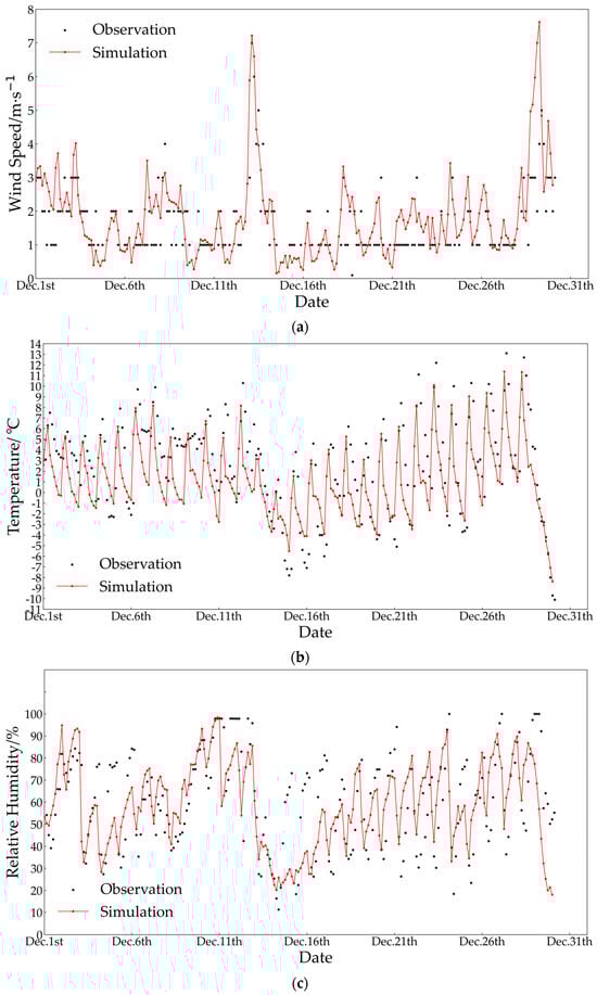

Figure 4.
Comparison between simulations and observations of meteorology in Xuzhou in December 2020 ((a–d) shows the simulations of wind speed, air temperature, relative humidity, and pressure, respectively, compared with observations; black dots represent meteorological observations, and red lines represent WRF simulations.
Table 4.
Statistical analysis of hourly meteorological observations and simulations for December 2020 in Xuzhou City.
Comparing the simulations of PM2.5 and PM10 concentration (Figure 2 and Figure 3) with the simulations of meteorology (Figure 4), it can be observed that the WS was lower before and during heavy pollution days (e.g., 11–12 December and 26–27 December) with large PM2.5 and PM10 concentrations, while the WS was higher after heavy pollution days (e.g., 12–13 December and 28–29 December). This better explains the process of increasing PM2.5 and PM10 concentrations due to the deposition of pollutants by low wind speeds before pollution, and decreasing due to the easy dispersion of pollutants as wind speeds increase. Simultaneously, we found that before the pollution process, there was a small increase in the temperature change and the air pressure was in a low-pressure state. With the end of the pollution process, the temperature gradually decreases and the air pressure gradually rises. This is also a side effect of the inversion and low-pressure environment that makes pollutants less likely to spread, allowing pollution to accumulate, leading to the formation of polluted days. At the same time, we found that the pollution process is accompanied by an increase in humidity, which leads to the settling of pollutants that are not easily dispersed. Overall, modeling and analyzing changes in meteorology over time can be vital in analyzing trends in pollutant concentrations.
3.3. Simulations on Heavily Polluted Days
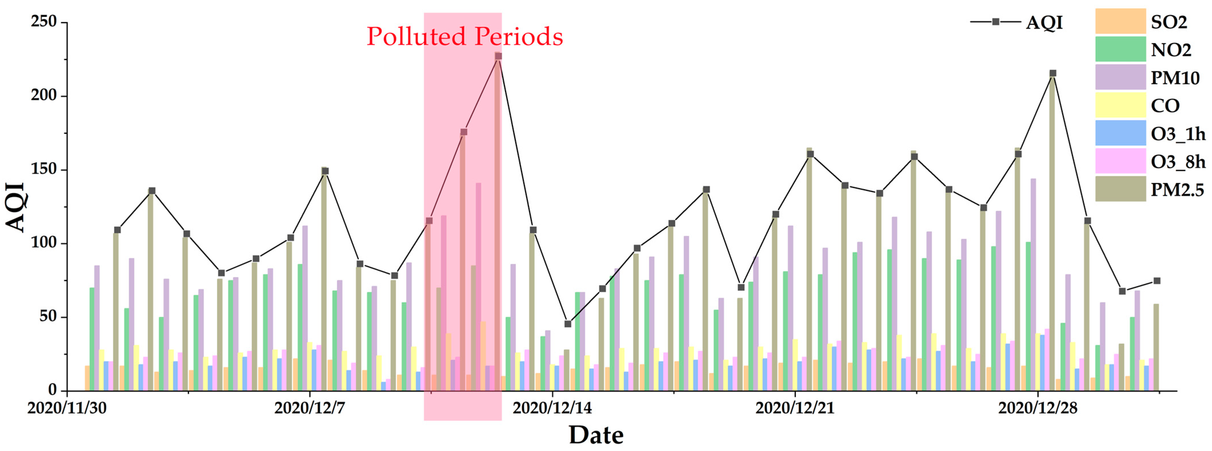
The study calculated the daily AQI index for the month of December 2020 in Xuzhou City (Figure 5). The study also calculated the IAQI for six pollutants (PM2.5, PM10, CO, O3, SO2, and NO2) and found that the IAQI for the PM2.5 pollutant was larger than the IAQI for the others on most days of the month. Therefore, it is necessary to study the characteristics of PM2.5 concentration changes. The experimentally calculated daily AQI indexes were compared and found that the AQI level of Xuzhou City was good on 9 December, mildly polluted on the 10th, moderately polluted on the 11th, heavily polluted on the 12th, and good on the 13th. The AQI was the highest on the 12th, and the observations showed that the PM2.5 concentration rose sharply from 10:00 on the 11th, reached the highest at 18:00 on the 12th, declined rapidly after the 13th, and then the whole pollution process was over. On 11–12 December 2020, the AQI suddenly increased and the PM2.5 concentration also increased significantly, so the following experiments will investigate the PM2.5 pollution distribution characteristics of Xuzhou City on these two days using the WRF-Chem model and the ADMS-Urban model.
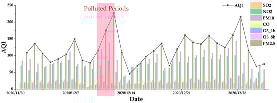
Figure 5.
Daily IAQI and AQI of each pollutant in Xuzhou City, December 2020.
3.3.1. WRF-Chem Simulations
The experiment was conducted to simulate the PM2.5 concentration from 10 to 13 December 2020 in Xuzhou City, and the simulations of the innermost layer of WRF-Chem for each 6-h period are shown in Figure 6. Comparing the PM2.5 concentration on 4 days, it can be seen that the PM2.5 concentration is higher from 18:00 on the 11th to 12:00 on the 12th in Xuzhou City, which is the time when the pollution process occurs. From 0:00 on the 10th, higher values of PM2.5 concentrations occurred only in a very small part of Xuzhou City, indicating that there was an accumulation of PM2.5 in some areas before the pollution occurred. Starting from 0:00 on the 11th, the PM2.5 concentration in the central area of Xuzhou City remained low. However, there was a noticeable increase in the PM2.5 concentration in the northern region of Xuzhou City, reaching levels as high as 220 μg/m3. As time progressed, the pollution area gradually shifted southward. Around 12:00 on the 11th, the PM2.5 concentration in the central area of Xuzhou City started to exhibit a gradual increase, while the PM2.5 concentration in the vicinity of the city center remained at a relatively low level. Until about 18:00 on the 11th, Xuzhou City, for the first time, showed a PM2.5 concentration greater than 200 μg/m3 of heavy air pollution phenomenon. At about 0:00 on the 12th, the PM2.5 concentration in the center of Xuzhou City was in the high concentration value in the vast majority of areas, with the highest concentration in the center and the concentration from the center to the surrounding gradient-decreasing phenomenon. At approximately 6:00 a.m. on the 12th, the PM2.5 concentration in Xuzhou City surged to extremely high levels. The simulated PM2.5 concentration in specific areas exceeded 260 μg/m3, resulting in a widespread region around Xuzhou City experiencing severe pollution. The PM2.5 concentration in Xuzhou City exhibited a gradual decrease from 12:00 to 18:00 on the 12th. By 0:00 on the 13th, the PM2.5 concentration had further decreased. By 12:00 on the 13th, the PM2.5 concentration had declined to below 80 μg/m3, marking the conclusion of the entire pollution event. At the time of pollution occurrence, localized areas in the northeastern part outside of Xuzhou were accompanied by a simultaneous increase in PM2.5 concentrations. As the pollution process ends, there is still an increase in PM2.5 concentrations in this area. It may be due to the rapid movement of PM2.5 air pollutants to the northeast as a result of the gradual increase in wind speed from the southwest during this period, resulting in the northeast part of the study area being affected by PM2.5 pollutants from Xuzhou City. In summary, the WRF-Chem model can better simulate PM2.5 concentration in Xuzhou City and the surrounding areas. The hourly temporal resolution allows for a more intuitive view of the changes in pollutant concentrations over time.
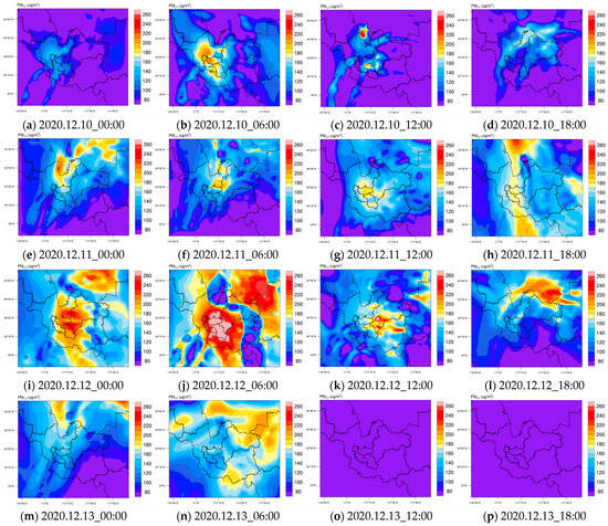
Figure 6.
WRF-Chem simulations of PM2.5 concentration in Xuzhou City from 10–13 December 2020. (a–d) are simulation results for 10 December; (e–h) are simulation results for 11 December; (i–l) are simulation results for 12 December; and (m–p) are simulation results for 13 December. (a,e,i,m) are simulation results at 6 a.m. on the same day; (b,f,j,n) are simulation results at 12 p.m. on the same day; (c,g,k,o) are simulation results at 18 p.m. on the same day; and (d,h,l,p) are simulation results at 0 a.m. on the following day.
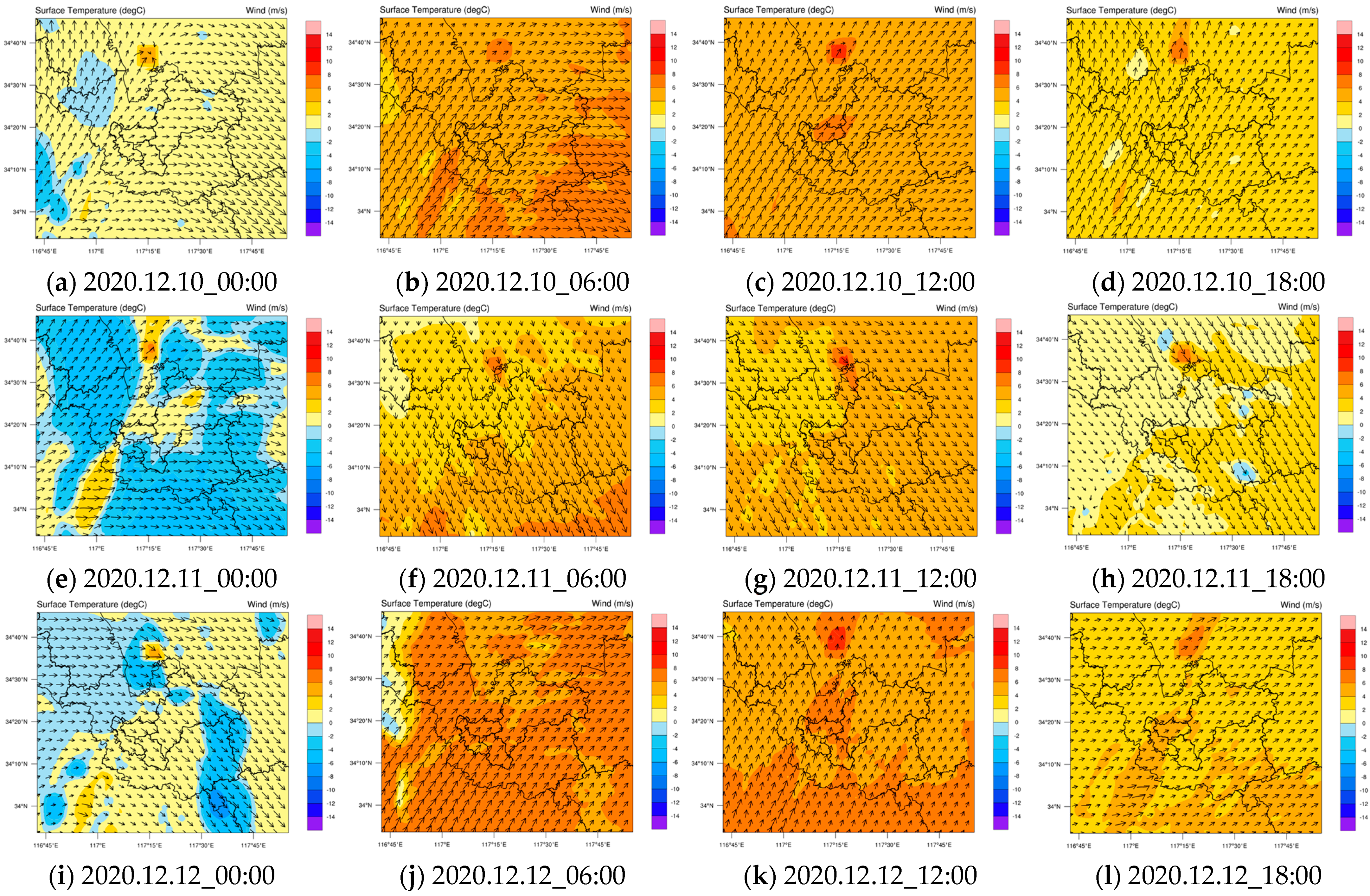
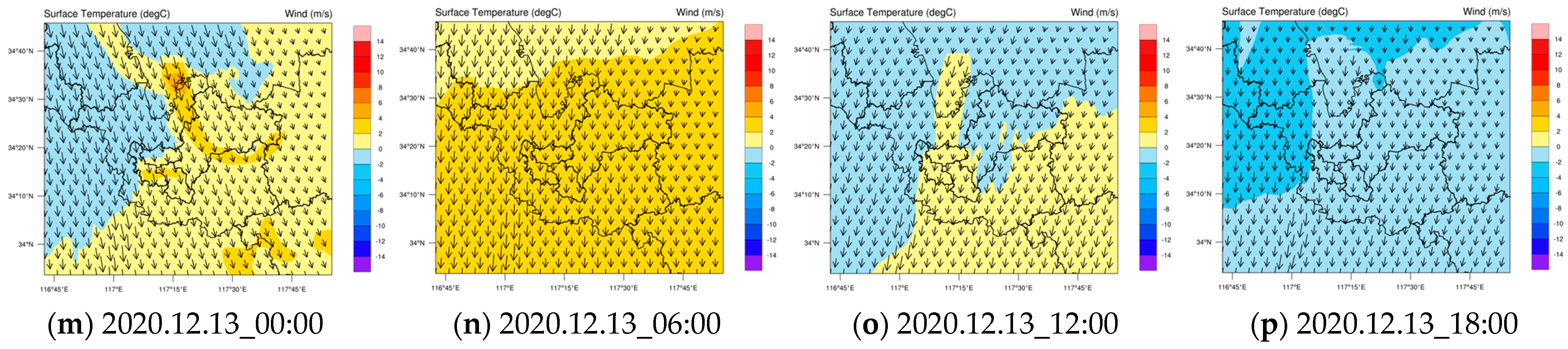
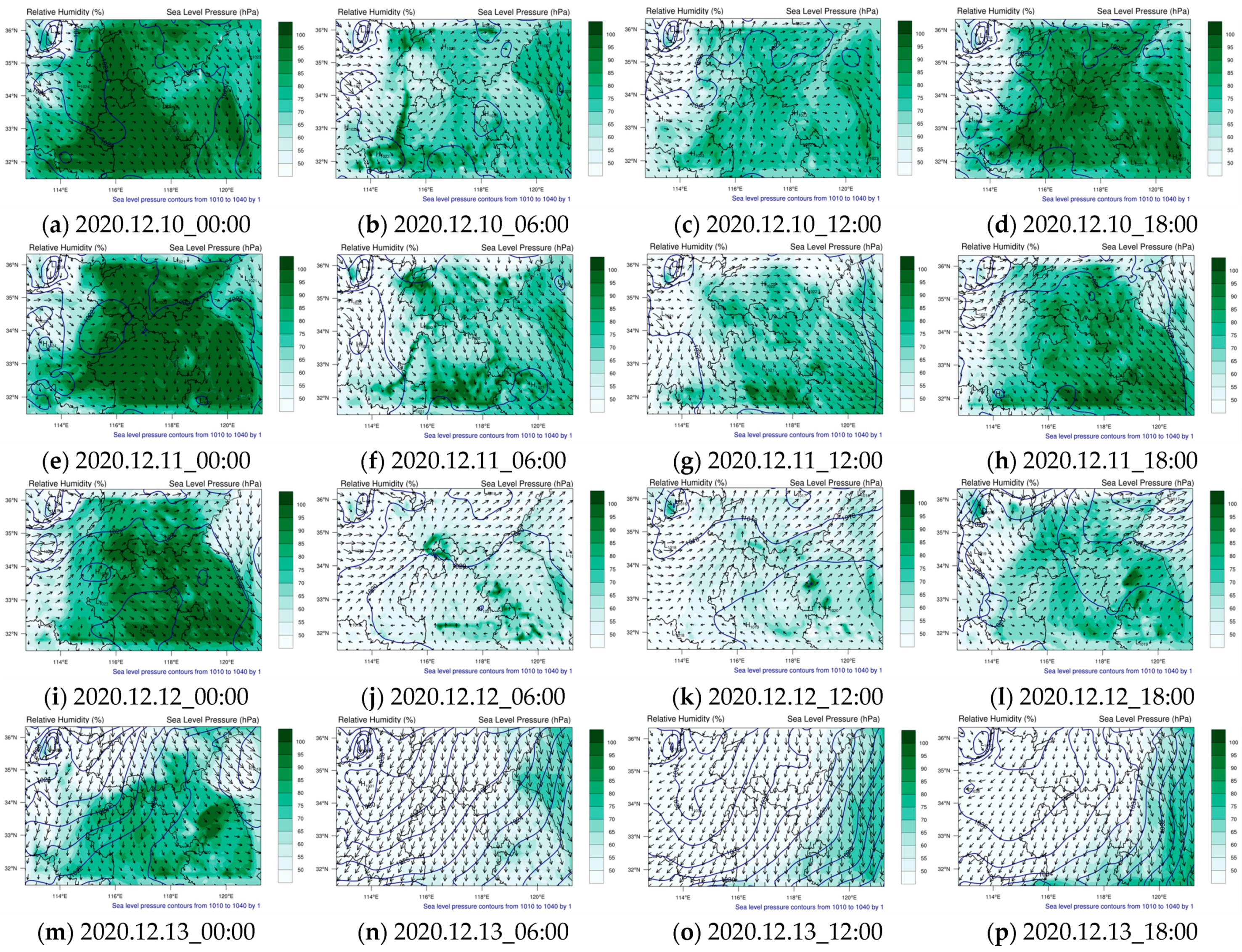
The experiment aimed to simulate the meteorological conditions of Xuzhou City from 10 to 13 December 2020. This included parameters such as temperature (T), relative humidity (RH), wind speed (WS), and pressure (P). The simulation results for each 6 h period are illustrated in Figure 7 (depicting the wind and temperature map) and Figure 8 (displaying the relative humidity and sea level pressure map) for the pollution process under consideration. Analyzing the simulations in Figure 7 alongside Figure 6, the temperature variations over the four days unfold as follows: During the daytime, T remains above 0 °C and exhibits a gradual increase over time. The highest value of T for the day is observed in the afternoon. At nighttime, T drops below 0 °C, reaching its lowest point around 6 o’clock the following day. The comparison of temperatures during the same time period on these four days reveals that T on the 12th was higher than that on the 10th and 11th, followed by a gradual decrease on the 13th. A gradual increase in T corresponds to the initiation of the pollution process. The accumulation of pollutants contributes to a gradual rise in surface temperature. Towards the conclusion of the pollution process, as the concentration of pollutants on the surface decreases, the surface temperature drops to lower values. The overall change in wind direction over the four days was a gradual shift from the southwest to the northwest before the pollution process, when pollutant concentrations gradually increased. As the wind shifted to the southwest again, the pollution process tended to end and the wind changed to the north. WS increased gradually over time, reaching a maximum on the 13th and decreasing on the 14th. Analyzing the simulations in Figure 8 alongside Figure 6, it is observed that the maximum RH values for the four moments studied occurred at 06:00 each day. Lower RH values were noted at 12:00 and 18:00 each day, with RH showing an increasing trend at 00:00 the following day. At 06:00 on the 11th, the relative humidity in Xuzhou City reached saturation, with some areas reaching 100%. Subsequently, the RH gradually declined over time, and by 12:00 on the 12th, the majority of the region experienced RH values below 60%, with only a few areas exhibiting higher values. The RH on the whole day of the 13th was significantly lower than that on the 12th. The increase in RH makes it easy for the pollutants to settle, which is one of the reasons why the pollution process occurs. The simulations of P during the pollution process range from 1018–1022 hpa, indicating that P tends to be roughly stable during the pollution process. At 0:00 on the 13th, P began to gradually rise. This suggests that low pressure makes pollutants gather and disperse less easily. The increase in pressure facilitates the flow of pollutants, signaling the conclusion of the pollution process.
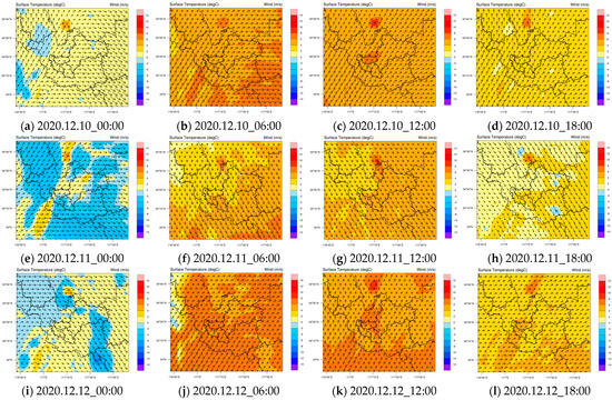
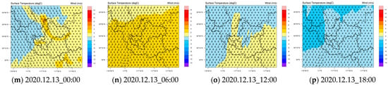
Figure 7.
WRF-Chem simulations of T and WS in Xuzhou, 10–13 December 2020. The presentation of (a–p) is the same as in Figure 5.
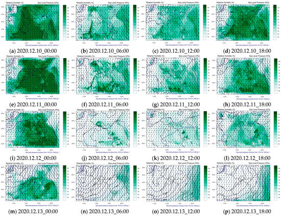
Figure 8.
WRF-Chem simulations of RH, P, and WS in Xuzhou City, 10–13 December 2020. The presentation of (a–p) is the same as in Figure 6.
In summary, this pollution process is characterized by a short process time and high pollution level. Combining the meteorological parameters simulated in Figure 7 and Figure 8 shows that the pollution process is controlled by the entire western airflow. Throughout the pollution event, the wind speed exhibited minimal variation. The wind direction, however, remained variable, fluctuating between the southwest, west, and northwest. In the polluted areas, the air pressure remains low. With the escalation of pollution, Xuzhou comes under the influence of weak high pressure. Eventually, the weather situation stabilizes as the pollution concentration decreases. According to the analysis of meteorological conditions, the wind speed of the pollution process is low, which is not conducive to the diffusion of pollutants, and the center of Xuzhou City is in a low-pressure state with high humidity, which exacerbates air pollution. With the gradual increase in central air pressure, at the end of the pollution process, the center of Xuzhou is in a state of high pressure with increasing wind speed and decreasing humidity and, ultimately, the pollution situation can be alleviated.
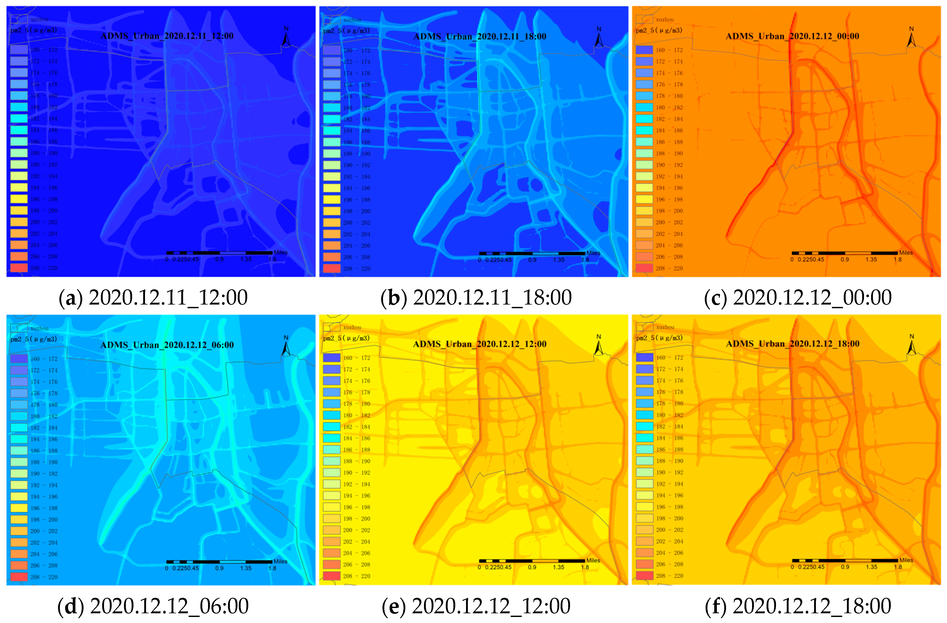
3.3.2. ADMS-Urban Simulations
Although WRF-Chem is a third-generation atmospheric transport model suitable for studying regional-scale air quality changes and can simulate the characteristics of PM2.5 concentration changes in local areas of Xuzhou, the simulation of pollutant concentrations at a higher spatial resolution is slightly lacking, also it is not possible to simulate the characteristics of the PM2.5 concentration distribution around buildings and roads in Xuzhou City. The ADMS-Urban model can deal with the complex terrain of urban areas, taking into account the effects of man-made structures such as buildings, streets, and roads on the wind field and airflow. The simulation accuracy of the WRF-Chem model for PM2.5 concentration on polluted days is slightly lacking, so in this study, the ADMS-Urban model was used to simulate the PM2.5 concentration in the central area of Xuzhou City every 6 h from 11 to 12 December 2020, and the results are shown in Figure 9. The spatial resolution of the simulation is 10 m, so the distribution characteristics and concentration changes of PM2.5 around roads and buildings in the three administrative districts of Quanshan District, Gulou District, and Yunlong District in the city center of Xuzhou can be clearly observed. It can be found that the distribution characteristics of PM2.5 concentration in Xuzhou present extremely high values on the roads and lower and consistent concentrations of pollutants around the roads, indicating that the ADMS-Urban model has a higher simulation accuracy of PM2.5 concentration on the roads. The increased PM2.5 concentrations on roads are likely associated with vehicle emissions. Furthermore, there seems to be a correlation between the width of the roadway and higher PM2.5 concentrations within the street, potentially linked to the elevated traffic volume on wider roads. Higher PM2.5 concentrations within downtown streets may result from the higher intensity of pollutant emission sources around downtown roadways. The dispersion distribution of PM2.5 around roads was found to be closely related to wind direction and wind speed. The wind direction of the pollution process is westerly, and the eastern concentration value of PM2.5 concentration around the roadway simulated with ADMS-Urban is significantly higher than the western value. The wind direction at 0:00 on the 12th was northwesterly, which is a more reasonable explanation for the fact that the PM2.5 concentration values in the eastern part of the road in Xuzhou City were significantly higher than the PM2.5 concentration values in the western parts. Meanwhile, the whole pollution process was accompanied by a gradual increase in WS, and the area of high PM2.5 concentrations east of the roadway was larger in the ADMS-Urban simulation at 18:00 on the 12th, which may be related to the persistence of larger westerly winds. In summary, the ADMS-Urban model can more accurately simulate the change in PM2.5 concentration at the road scale in the center of Xuzhou City, and can better simulate the distribution characteristics of PM2.5 concentration around the roads and buildings, which is helpful for the study of the spatial and temporal distribution characteristics of pollutants at a high spatial resolution in the city.
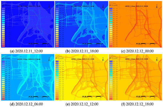
Figure 9.
ADMS-Urban simulations of PM2.5 concentration in Xuzhou on 11–12 December 2020. Figures (a–f) show simulation results at 6 h intervals from 12:00 p.m. on 11 December 2020 to 18:00 p.m. on 12 December 2020.
4. Discussion
The results of our study were compared with those of Jin Wang [62] and Qiao et al. [14]. The experiments of Wang and Qiao et al. were simulated using the WRF-Chem model by selecting Xuzhou City and Guangzhou City as their respective study areas. The R of our simulations for P, T, and RH are 0.99, 0.89, and 0.71, respectively, which are all within the range of the month-by-month meteorology simulated by Wang of 0.97–0.99, 0.73–0.89, and 0.61–0.78 and the results of the T and RH simulations by Qiao et al.
The R values of 0.95 and 0.88, respectively, are better than ours, which may be related to the fact that the WRF-Chem model simulates meteorology variously for different seasons. The WS simulated by us (R of 0.75) is better than the results simulated by Wang and Qiao et al. (R of 0.52–0.66 and 0.64, respectively), while the PM2.5 concentration simulated by us (R of 0.63) is similar to the results simulated by Wang (R of 0.47–0.68).
The results of the study were compared with those of Wen et al. [63], whose experiments also used the WRF-Chem and ADMS-Urban models to carry out high-resolution simulations of air pollution at the urban scale for typical pollution cases. Wen et al. set five nested layers with an innermost spatial resolution of 1 km, which is the same accuracy as the innermost nesting studied in this paper. In comparing the simulation results of PM2.5 pollutant concentration, Wen et al. reported an RMSE of 32.78, while this experiment yielded an RMSE of 39.23. These values indicate substantial uncertainties within the present experimental study, resulting in notable differences in the simulation outcomes. Both sides selected polluted and clean days, respectively, to compare the simulated PM2.5 concentrations, and the WRF-Chem model simulated PM2.5 concentrations on polluted days worse than on clean days, with larger RMSE and MB of PM2.5 concentrations on polluted days, indicating that the model was weaker in simulating PM2.5 concentrations on heavily polluted days. In this paper, the influence of meteorology on PM2.5 concentrations as simulated with WRF is considered, whereas the analysis of meteorological simulations was missing in the study by Wen et al. The influence of streets and buildings on the simulation was taken into account in both experimental setups of the ADMS-Urban model. Wen et al. chose the extent of the study area in the same way as the innermost study area of the WRF-Chem model and used the average of the meteorological conditions obtained from the WRF-Chem simulations as the meteorological input data for the ADMS. Due to constraints, this experiment selected the downtown area as the research region, and the meteorological input data were sourced from the ERA5 reanalysis dataset. The focused nature of this small-scale research experiment allows for a more accurate depiction of the distribution of PM2.5 concentrations around roadways. Although the results of Wen et al. can visualize the distribution of PM2.5 concentration around the main roads, the simulation on the detailed roads in the city is poor, whereas, in this experiment, a small area in the city center is selected for high-resolution air pollutant simulation, which makes the experimental results more accurate.
The WRF-Chem model was used to simulate the pollutant concentrations in Xuzhou City in December 2020, and this approach was successfully implemented in this paper by using the ADMS-Urban model for the refinement of the study of heavy pollution days where there were large deviations in the simulation of pollutant concentrations. However, the experiment may have some limitations: The WRF-Chem model appears to employ a nested study approach for regional air quality simulations. This involves multiple layers of nested studies, likely indicating a hierarchical or refined spatial resolution. This approach may enhance the model’s ability to capture localized variations in air quality but may come at the cost of increased computational time. In contrast, the ADMS-Urban model seems to focus more on detailed data related to road pollutant emissions, road widths, valley heights, and possibly other factors influencing urban air quality. This suggests a more localized and specific approach, emphasizing the importance of detailed input data for accurate simulations at the urban scale, while it is more difficult to obtain the data required for the ADMS-Urban model in some cities with complex terrain or in some large cities with a lot of information on roads and buildings. WRF-Chem’s nested studies may lead to longer simulation times, making it suitable for broader regional analyses. Meanwhile, ADMS-Urban’s focus on detailed data may reduce computational demands but requires comprehensive input information. WRF-Chem’s nested structure may provide higher spatial resolution, capturing fine-scale variations. ADMS-Urban, by focusing on urban factors, may excel in modeling localized effects within urban environments. Further research is necessary to determine the applicability of the methodology developed in this study to diverse urban environments.
Based on the above comparative discussion and reflection on the experimental process, we have the following outlook: (1) Experiments were conducted to investigate the spatial and temporal distribution of PM2.5 concentrations in Xuzhou. The study utilized both the WRF-Chem and ADMS-Urban models, and comparative discussions were undertaken to analyze their respective findings. The two models have their own advantages, and how to couple them is the goal of the next work. The results of the innermost nested simulations of WRF-Chem are used as background fields for the ADMS-Urban model, allowing for a more refined study. However, the disadvantage of this method is that the computational work is huge and time-consuming, so there is a need to find a more suitable method to solve the problem of how to model air pollutants with high accuracy and efficiency. (2) The experiment investigates the PM2.5 concentration on roads in Xuzhou through the ADMS-Urban model, but lacks a more detailed study of the PM2.5 concentration around major buildings and large industrial bases. Therefore, how to study the concentration of pollutants in Xuzhou with a higher resolution as well as refine the PM2.5 concentration in complex conditions such as towns, cities, highways, and large industrial bases become the next major research objectives. (3) The accuracy of the anthropogenic emission data and biogenic emission data added to the WRF-Chem simulation of PM2.5 concentration in the experiment is rather general, and it is worthwhile to study how to add more quantitative data. Some scholars have replaced the land use data in the WRF model with self-produced categorized subsurface data, which makes the research results more accurate. (4) At present, remote sensing plays an increasingly important role in the study of the environment, and it is worthwhile for us to study and discuss how to incorporate satellite observation data into WRF-Chem in order to improve the accuracy of the model simulation. Meanwhile, the assimilation of the simulation results of the numerical atmospheric prediction model with the observations from satellite remote sensing data can further improve the simulation’s accuracy of atmospheric pollutants.
5. Conclusions
The study of the spatial distribution and pollution characteristics of PM2.5 is necessary for the study of urban air quality changes, and how to quickly and accurately simulate the pollutant concentration changes and spatial and temporal distributions is a hot topic of research nowadays. In this paper, we decided to use the WRF-Chem model and ADMS-Urban model to study the characteristics of meteorology and PM2.5 concentration in December 2020 in Xuzhou City. The WRF-Chem model was first used to identify the heavy pollution days and pollution areas, and then the ADMS-Urban model was used to refine the simulation for localized areas. The conclusions of the study are as follows:
(1) The study first simulates the meteorology in Xuzhou including temperature (T), relative humidity (RH), wind speed (WS), and pressure (P) using the WRF-Chem model with R ranging from 0.71–0.99, and the meteorology simulated with the WRF-Chem model embody a better simulation result. Combined with the analysis of the IAQI of various air pollutants in Xuzhou in December 2020, it was determined that the top air pollutant in Xuzhou this month was PM2.5. The WRF-Chem model was used to simulate the PM2.5 concentration and it was found that the simulations were generally consistent with the observations (R of 0.63). The WRF-Chem model exhibits an underestimation of PM2.5 concentration during severe air pollution days. Through an analysis of meteorological simulations using the WRF-Chem model, it was observed that the spatial distribution of PM2.5 concentration from 10–13 December indicated a movement of the high-value area from the southwest to the northeast, with a pronounced concentration over Xuzhou. As the air pressure in the center of Xuzhou City changed from low pressure to weak high pressure, accompanied by the increase in wind speed from the west, the pollutant concentration gradually decreased and the whole pollution process ended;
(2) Given the inherent bias of the WRF-Chem model in simulating results during heavy pollution days in Xuzhou City, and its limitation in depicting the spatial and temporal changes and distribution characteristics of PM2.5 concentration around streets and buildings, this study opted to simulate the PM2.5 concentration in the central area of Xuzhou City during heavy pollution days on 11–12 December using the ADMS-Urban model. The findings vividly depicted the spatial distribution of PM2.5 concentration surrounding roadways. The results unequivocally indicated elevated PM2.5 concentrations in proximity to roads, with higher values observed on broader roads and within the city center area. It was also found that the PM2.5 concentration was closely related to the downwind direction. With mainly westerly winds during the study period, the road PM2.5 concentrations in the eastern part simulated with ADMS-Urban were significantly higher than those in the western part;
(3) Combining the results of the two models, the WRF-Chem model can better simulate the distribution characteristics of PM2.5 concentration in Xuzhou and its surrounding areas, and more intuitively derive the movement trend of pollutants and their sources. The ADMS-Urban model takes into account complex topography such as streets and buildings, and the model itself inputs more emission data, making it more suitable for studying changes in air pollutant concentrations in small urban areas. Therefore, how to combine the two models more closely to study the variation in urban air pollutant concentrations, or to put the initial results of the WRF-Chem model simulation into the ADMS-Urban model to continue the simulation, is the next research direction.
Author Contributions
Conceptualization, W.L., X.L. and Y.X.; methodology, W.L. and S.W.; validation, W.L., X.L. and Y.X.; formal analysis, W.L.; investigation, W.L.; resources, W.L. and J.G.; data curation, W.L. and S.W.; writing—original draft preparation, W.L.; writing—review and editing, W.L., X.L. and Y.X.; visualization, W.L.; supervision, L.Z. and B.H.; funding acquisition, Y.X., X.L. and L.Z. All authors have read and agreed to the published version of the manuscript.
Funding
This work was jointly funded by the National Natural Science Foundation of China (Grant No. 42275147, 42075114, 41705101), the Priority Academic Program Development of Jiangsu Higher Education Institutions (140119001), the Research and Demonstration of Fine Numerical Simulation of Atmospheric Pollution and Greenhouse Gases in Xuzhou City (KC22108), and the General Project of Modern Agriculture from the Primary R&D Program of Xuzhou (KC21132).
Institutional Review Board Statement
Not applicable.
Informed Consent Statement
Not applicable.
Data Availability Statement
Data sharing is not applicable to this article, as no new data were created or analyzed in this study.
Acknowledgments
The authors are very grateful for the comments and remarks of the reviewers who helped to improve the manuscript. Thanks to the editors for all their work on this manuscript.
Conflicts of Interest
The authors declare no conflicts of interest.
References
- Tian, Y.; He, C.; Yang, L.; Yi, J.H.; Ke, B.Q.; Mu, H.; Tu, P.Y.; Ye, Z.X.; Hong, S. Spatiotemporal Dynamic Correlation Characteristics and Driving Factors of Major Air Pollutant Emissions in China. Atmosphere 2023, 14, 130. [Google Scholar] [CrossRef]
- Li, X.J.; Hussain, S.A.; Sobri, S.; Said, M. Overviewing the air quality models on air pollution in Sichuan Basin, China. Chemosphere 2021, 271, 129502. [Google Scholar] [CrossRef] [PubMed]
- Jia, Z.X.; Doherty, R.M.; Ordóñez, C.; Li, C.F.; Wild, O.; Jain, S.; Tang, X. The impact of large-scale circulation on daily fine particulate matter (PM2.5) over major populated regions of China in winter. Atmos. Chem. Phys. 2022, 22, 6471–6487. [Google Scholar] [CrossRef]
- Geng, G.N.; Zheng, Y.X.; Zhang, Q.; Xue, T.; Zhao, H.Y.; Tong, D.; Zheng, B.; Li, M.; Liu, F.; Hong, C.P.; et al. Drivers of PM2.5 air pollution deaths in China 2002–2017. Nat. Geosci. 2021, 14, 645. [Google Scholar] [CrossRef]
- Yang, Y.; Ren, L.L.; Wu, M.X.; Wang, H.L.; Song, F.F.; Leung, L.R.; Hao, X.; Li, J.D.; Chen, L.; Li, H.M.; et al. Abrupt emissions reductions during COVID-19 contributed to record summer rainfall in China. Nat. Commun. 2022, 13, 959. [Google Scholar] [CrossRef] [PubMed]
- Zou, J.A.; Cao, Q.M.; Gao, W.K.; Liu, Z.R.; Wang, H.L.; Hu, B.; Wang, Y.S. The effects of number and mass concentration of aerosol components on scattering coefficients in Xianghe, southeast of Beijing, China-A case study. Atmos. Environ. 2022, 272, 118938. [Google Scholar] [CrossRef]
- Sokhi, R.S.; Moussiopoulos, N.; Baklanov, A.; Bartzis, J.; Coll, I.; Finardi, S.; Friedrich, R.; Geels, C.; Grönholm, T.; Halenka, T.; et al. Advances in air quality research—Current and emerging challenges. Atmos. Chem. Phys. 2022, 22, 4615–4703. [Google Scholar] [CrossRef]
- Wang, X.Y.; Zhang, R.H. Effects of atmospheric circulations on the interannual variation in PM2.5 concentrations over the Beijing-Tianjin-Hebei region in 2013–2018. Atmos. Chem. Phys. 2020, 20, 7667–7682. [Google Scholar] [CrossRef]
- Tang, M.F.; Wu, X.; Agrawal, P.; Pongpaichet, S.; Jain, R. Integration of Diverse Data Sources for Spatial PM2.5 Data Interpolation. IEEE Trans. Multimed. 2017, 19, 408–417. [Google Scholar] [CrossRef]
- Kukkonen, J.; Olsson, T.; Schultz, D.M.; Baklanov, A.; Klein, T.; Miranda, A.I.; Monteiro, A.; Hirtl, M.; Tarvainen, V.; Boy, M.; et al. A review of operational, regional-scale, chemical weather forecasting models in Europe. Atmos. Chem. Phys. 2012, 12, 1–87. [Google Scholar] [CrossRef]
- Bohnenstengel, S.I.; Belcher, S.E.; Aiken, A.; Allan, J.D.; Allen, G.; Bacak, A.; Bannan, T.J.; Barlow, J.F.; Beddows, D.; Bloss, W.J.; et al. Meteorology, Air Quality, and Health in London: The ClearfLo Project. Bull. Am. Meteorol. Soc. 2015, 96, 779–804. [Google Scholar] [CrossRef]
- Yang, X.Y.; Wu, K.; Wang, H.L.; Liu, Y.M.; Gu, S.; Lu, Y.Q.; Zhang, X.L.; Hu, Y.S.; Ou, Y.H.; Wang, S.G.; et al. Summertime ozone pollution in Sichuan Basin, China: Meteorological conditions, sources and process analysis. Atmos. Environ. 2020, 226, 117392. [Google Scholar] [CrossRef]
- Shukla, K.K.; Attada, R.; Khan, A.W.; Kumar, P. Evaluation of extreme dust storm over the northwest Indo-Gangetic plain using WRF-Chem model. Nat. Hazards 2022, 110, 1887–1910. [Google Scholar] [CrossRef]
- Qiao, Z.; Cui, S.C.; Pei, C.L.; Ye, Z.; Wu, X.Q.; Lei, L.; Luo, T.; Zhang, Z.H.; Li, X.B.; Zhu, W.Y. Regional Predictions of Air Pollution in Guangzhou: Preliminary Results and Multi-Model Cross-Validations. Atmosphere 2022, 13, 1527. [Google Scholar] [CrossRef]
- Shahid, M.Z.; Chishtie, F.; Bilal, M.; Shahid, I. WRF-Chem Simulation for Modeling Seasonal Variations and Distributions of Aerosol Pollutants over the Middle East. Remote Sens. 2021, 13, 2112. [Google Scholar] [CrossRef]
- Do, T.; Ngo, X.T.; Pham, V.H.; Vuong, N.L.; Le, H.A.; Pham, C.T.; Bui, Q.H.; Nguyen, T. Application of WRF-Chem to simulate air quality over Northern Vietnam. Environ. Sci. Pollut. Res. 2021, 28, 12067–12081. [Google Scholar] [CrossRef]
- Rostkier-Edelstein, D.; Kunin, P.; Sheu, R.S.; Gelman, A.; Yunker, A.; Roux, G.; Pietrkowski, A.; Zhang, Y.X. Evaluation of WRF-Chem-RTFDDA dust forecasts over the MENA region using in-situ and remote-sensing observations. Front. Environ. Sci. 2022, 10, 1747. [Google Scholar] [CrossRef]
- Georgiou, G.K.; Christoudias, T.; Proestos, Y.; Kushta, J.; Pikridas, M.; Sciare, J.; Savvides, C.; Lelieveld, J. Evaluation of WRF-Chem model (v3.9.1.1) real-time air quality forecasts over the Eastern Mediterranean. Geosci. Model Dev. 2022, 15, 4129–4146. [Google Scholar] [CrossRef]
- Owen, B.; Edmunds, H.A.; Carruthers, D.J.; Singles, R.J. Prediction of total oxides of nitrogen and nitrogen dioxide concentrations in a large urban area using a new generation urban scale dispersion model with integral chemistry model. Atmos. Environ. 2000, 34, 397–406. [Google Scholar] [CrossRef]
- He, B.; Heal, M.R.; Humstad, K.H.; Yan, L.; Zhang, Q.; Reis, S. A hybrid model approach for estimating health burden from NO2 in megacities in China: A case study in Guangzhou. Environ. Res. Lett. 2019, 14, 124019. [Google Scholar] [CrossRef]
- Munir, S.; Habeebullah, T.M. Vehicular emissions on main roads in Makkah, Saudi Arabiaa dispersion modelling study. Arab. J. Geosci. 2018, 11, 531. [Google Scholar] [CrossRef]
- Dimitrova, R.; Velizarova, M. Assessment of the Contribution of Different Particulate Matter Sources on Pollution in Sofia City. Atmosphere 2021, 12, 423. [Google Scholar] [CrossRef]
- Biggart, M.; Stocker, J.; Doherty, R.M.; Wild, O.; Hollaway, M.; Carruthers, D.; Li, J.; Zhang, Q.; Wu, R.L.; Kotthaus, S.; et al. Street-scale air quality modelling for Beijing during a winter 2016 measurement campaign. Atmos. Chem. Phys. 2020, 20, 2755–2780. [Google Scholar] [CrossRef]
- Ukhov, A.; Mostamandi, S.; Da Silva, A.; Flemming, J.; Alshehri, Y.; Shevchenko, I.; Stenchikov, G. Assessment of natural and anthropogenic aerosol air pollution in the Middle East using MERRA-2, CAMS data assimilation products, and high-resolution WRF-Chem model simulations. Atmos. Chem. Phys. 2020, 20, 9281–9310. [Google Scholar] [CrossRef]
- Zhong, J.; Hood, C.; Johnson, K.; Stocker, J.; Handley, J.; Wolstencroft, M.; Mazzeo, A.; Cai, X.M.; Bloss, W.J. Using Task Farming to Optimise a Street-Scale Resolution Air Quality Model of the West Midlands (UK). Atmosphere 2021, 12, 983. [Google Scholar] [CrossRef]
- Westmoreland, E.J.; Carslaw, N.; Carslaw, D.C.; Gillah, A.; Bates, E. Analysis of air quality within a street canyon using statistical and dispersion modelling techniques. Atmos. Environ. 2007, 41, 9195–9205. [Google Scholar] [CrossRef]
- Zhang, Y.X.; Olsen, S.C.; Dubey, M.K. WRF/Chem simulated springtime impact of rising Asian emissions on air quality over the US. Atmos. Environ. 2010, 44, 2799–2812. [Google Scholar] [CrossRef]
- Grell, G.A.; Peckham, S.E.; Schmitz, R.; Mckeen, S.A.; Frost, G.; Skamarock, W.C.; Eder, B. Fully coupled “online” chemistry within the WRF model. Atmos. Environ. 2005, 39, 6957–6975. [Google Scholar] [CrossRef]
- Chapman, E.G.; Gustafson, W.I.; Easter, R.C.; Barnard, J.C.; Ghan, S.J.; Pekour, M.S.; Fast, J.D. Coupling aerosol-cloud-radiative processes in the WRF-Chem model: Investigating the radiative impact of elevated point sources. Atmos. Chem. Phys. 2009, 9, 945–964. [Google Scholar] [CrossRef]
- Stockwell, W.R.; Middleton, P.; Chang, J.S.; Tang, X. The second generation regional acid deposition model chemical mechanism for regional air quality modeling. J. Geophys. Res.-Atmos. 1990, 95, 16343–16367. [Google Scholar] [CrossRef]
- Seefeld, W.R.S.K. A new mechanism for regional atmospheric chemistry modeling. J. Geophys. Res.-Atmos. 1997, 102, 25847–25879. [Google Scholar]
- Zaveri, R.A.; Peters, L.K. A new lumped structure photochemical mechanism for large-scale applications. J. Geophys. Res.-Atmos. 1999, 104, 30387–30415. [Google Scholar] [CrossRef]
- Gery, M.W.; Whitten, G.Z.; Killus, J.P.; Dodge, M.C. A photochemical kinetics mechanism for urban and regional scale computer modeling. J. Geophys. Res. 1989, 94, 12925–12956. [Google Scholar] [CrossRef]
- Yarwood, G.; Rao, S.; Yocke, M.; Whitten, G. Updates to the Carbon Bond Chemical Mechanism: CB05 Final Report to the US EPA; EPA: Washington, DC, USA, 2005.
- Carter. Implementation of the SAPRC-99 Chemical Mechanism into the Models-3 Framework; Carter: Atlanta, GA, USA, 2000. [Google Scholar]
- Ij, A.; Memmesheimer, M.; Ebel, A.; Fs, B.; Shankar, U.; Hass, H. Modal aerosol dynamics model for Europe: Development and first applications. Atmos. Environ. 1998, 32, 2981–2999. [Google Scholar]
- Schell, B.; Ackermann, I.J.; Hass, H.; Binkowski, F.S.; Ebel, A. Modeling the formation of secondary organic aerosol within a comprehensive air quality model system. J. Geophys. Res.-Atmos. 2001, 106, 28275–28293. [Google Scholar] [CrossRef]
- Ahmadov, R.; Mckeen, S.A.; Robinson, A.L.; Bahreini, R.; Middlebrook, A.M.; Gouw, J.A.D.; Meagher, J.; Hsie, E.Y.; Edgerton, E.; Shaw, S. A volatility basis set model for summertime secondary organic aerosols over the eastern United States in 2006. J. Geophys. Res.-Atmos. 2012, 117, 6301. [Google Scholar] [CrossRef]
- Liu, X.; Easter, R.C.; Ghan, S.J.; Zaveri, R.; Rasch, P.; Shi, X.; Lamarque, J.F.; Gettelman, A.; Morrison, H.; Vitt, F.; et al. Toward a minimal representation of aerosols in climate models: Description and evaluation in the Community Atmosphere Model CAM5. Geosci. Model Dev. 2012, 5, 709–739. [Google Scholar] [CrossRef]
- Zaveri, R.A.; Easter, R.C.; Fast, J.D.; Peters, L.K. Model for Simulating Aerosol Interactions and Chemistry (MOSAIC). J. Geophys. Res.-Atmos. 2008, 113, D13204. [Google Scholar] [CrossRef]
- Chin, M.; Ginoux, P.; Kinne, S.; Torres, O.; Holben, B.N.; Duncan, B.N.; Martin, R.V.; Logan, J.A.; Higurashi, A.; Nakajima, T. Tropospheric aerosol optical thickness from the GOCART model and comparisons with satellite and Sun photometer measurements. J. Atmos. Sci. 2002, 59, 461–483. [Google Scholar] [CrossRef]
- Chen, S.H.; Sun, W.Y. A one-dimensional time dependent cloud model. J. Meteorol. Soc. Jpn. 2002, 80, 99–118. [Google Scholar] [CrossRef]
- Grell, G.A.; Dévényi, D. A generalized approach to parameterizing convection combining ensemble and data assimilation techniques. Geophys. Res. Lett. 2002, 29, 38-1–38-4. [Google Scholar] [CrossRef]
- Ej, M.; Pd, B.; Mj, I.; Sa, C.; Sj, T. Radiative transfer for inhomogeneous atmospheres—RRTM, a validated correlated-k model for the longwave. J. Geophys. Res. Atmos. 1997, 102, 16663–16682. [Google Scholar]
- Matsui, T.; Zhang, S.Q.; Lang, S.E.; Tao, W.K.; Ichoku, C.; Peters-Lidard, C.D. Impact of radiation frequency, precipitation radiative forcing, and radiation column aggregation on convection-permitting West African monsoon simulations. Clim. Dynam. 2020, 55, 193–213. [Google Scholar] [CrossRef]
- Jiménez, P.A.; Dudhia, J.; González-Rouco, J.F.; Navarro, J.; Montávez, J.P.; García-Bustamante, E. A Revised Scheme for the WRF Surface Layer Formulation. Mon. Weather Rev. 2012, 140, 898–918. [Google Scholar] [CrossRef]
- Weston, M.; Chaouch, N.; Valappil, V.; Temimi, M.; Ek, M.; Zheng, W.Z. Assessment of the Sensitivity to the Thermal Roughness Length in Noah and Noah-MP Land Surface Model Using WRF in an Arid Region. Pure Appl. Geophys. 2019, 176, 2121–2137. [Google Scholar] [CrossRef]
- Hong, S.Y.; Noh, Y.; Dudhia, J. A new vertical diffusion package with an explicit treatment of entrainment processes. Mon. Weather Rev. 2006, 134, 2318–2341. [Google Scholar] [CrossRef]
- Wild, O.; Zhu, X.; Prather, M.J. Fast-J: Accurate Simulation of In- and Below-Cloud Photolysis in Tropospheric Chemical Models. J. Atmos. Chem. 2000, 37, 245–282. [Google Scholar] [CrossRef]
- National Centers For Environmental Prediction; National Weather Service; NOAA; U.S. Department of Commerce. NCEP FNL Operational Model Global Tropospheric Analyses, Continuing from July 1999; Research Data Archive at the National Center for Atmospheric Research, Computational and Information Systems Laboratory: Boulder, CO, USA, 2000.
- Lamarque, J.F.; Emmons, L.K.; Hess, P.G.; Kinnison, D.E.; Tilmes, S.; Vitt, F.; Heald, C.L.; Holland, E.A.; Lauritzen, P.H.; Neu, J.; et al. CAM-chem: Description and evaluation of interactive atmospheric chemistry in the Community Earth System Model. Geosci. Model Dev. 2012, 5, 369–411. [Google Scholar] [CrossRef]
- Guenther, A.B.; Jiang, X.; Heald, C.L.; Sakulyanontvittaya, T.; Duhl, T.; Emmons, L.K.; Wang, X. The Model of Emissions of Gases and Aerosols from Nature version 2.1 (MEGAN2.1): An extended and updated framework for modeling biogenic emissions. Geosci. Model Dev. 2012, 5, 1471–1492. [Google Scholar] [CrossRef]
- Li, M.; Liu, H.; Geng, G.N.; Hong, C.P.; Liu, F.; Song, Y.; Tong, D.; Zheng, B.; Cui, H.Y.; Man, H.Y.; et al. Anthropogenic emission inventories in China: A review. Natl. Sci. Rev. 2017, 4, 834–866. [Google Scholar] [CrossRef]
- Zheng, B.; Tong, D.; Li, M.; Liu, F.; Hong, C.P.; Geng, G.N.; Li, H.Y.; Li, X.; Peng, L.Q.; Qi, J.; et al. Trends in China’s anthropogenic emissions since 2010 as the consequence of clean air actions. Atmos. Chem. Phys. 2018, 18, 14095–14111. [Google Scholar] [CrossRef]
- Mchugh, C.A.; Carruthers, D.J.; Edmunds, H.A. ADMS-Urban: An air quality management system for traffic, domestic and industrial pollution. Int. J. Environ. Pollut. 1997, 8, 666–674. [Google Scholar]
- Stocker, J.; Hood, C.; Carruthers, D.; Mchugh, C. ADMS-Urban: Developments in modelling dispersion from the city scale to the local scale. Int. J. Environ. Pollut. 2012, 50, 308–316. [Google Scholar] [CrossRef]
- Righi, S.; Lucialli, P.; Pollini, E. Statistical and diagnostic evaluation of the ADMS-Urban model compared with an urban air quality monitoring network. Atmos. Environ. 2009, 43, 3850–3857. [Google Scholar] [CrossRef]
- Jiang, Z.X.; Gao, Y.C.; Cao, H.X.; Diao, W.X.; Yao, X.; Yuan, C.C.; Fan, Y.Y.; Chen, Y. Characteristics of ambient air quality and its air quality index (AQI) model in Shanghai, China. Sci. Total Environ. 2023, 896, 165284. [Google Scholar] [CrossRef] [PubMed]
- Falzone, C.; Romain, A.C. Establishing an Air Quality Index Based on Proxy Data for Urban Planning Part 1: Methodological Developments and Preliminary Tests. Atmosphere 2022, 13, 1470. [Google Scholar] [CrossRef]
- Li, Y.P.; Tang, Y.; Fan, Z.Y.; Zhou, H.; Yang, Z.Z. Assessment and comparison of three different air quality indices in China. Environ. Eng. Res. 2018, 23, 21–27. [Google Scholar] [CrossRef]
- Chen, W.; Wang, F.S.; Xiao, G.F.; Wu, K.; Zhang, S.X. Air Quality of Beijing and Impacts of the New Ambient Air Quality Standard. Atmosphere 2015, 6, 1243–1258. [Google Scholar] [CrossRef]
- Jin, W. Study on PM2.5 Pollution over Xuzhou Using WRF-Chem. Master’s Thesis, China University of Mining and Technology, Xuzhou, China, 2017. [Google Scholar]
- Wen, J.K.; Wang, T.J.; Ma, G.H.; Sheng, X.Y.; Wang, Y.Z.; Lu, X.B.; Xiang, H.J.; Wu, D.L.; Li, G.M. Comparison between WRF-Chem and ADMS in the refined simulation of urban scale air pollution. Acta Sci. Circumstantiae 2022, 42, 276–292. [Google Scholar] [CrossRef]

Disclaimer/Publisher’s Note: The statements, opinions and data contained in all publications are solely those of the individual author(s) and contributor(s) and not of MDPI and/or the editor(s). MDPI and/or the editor(s) disclaim responsibility for any injury to people or property resulting from any ideas, methods, instructions or products referred to in the content. |
© 2024 by the authors. Licensee MDPI, Basel, Switzerland. This article is an open access article distributed under the terms and conditions of the Creative Commons Attribution (CC BY) license (https://creativecommons.org/licenses/by/4.0/).