Abstract
This study simulated the wind energy density distribution in the Jiaodong Peninsula region using the Weather Research and Forecasting (WRF) Model. The impacts of different boundary-layer and near-surface parameterization schemes on the simulated wind speed and direction were investigated. The results indicate that the Yonsei University (YSU) scheme and the Quasi-Normal Scale Elimination (QNSE) scheme performed optimally for wind speed and wind direction. We also conducted a sensitivity test of the simulation results for atmospheric pressure, air temperature, and relative humidity. The statistical analysis showed that the YSU scheme performed optimally, while the MRF and BL schemes performed poorly. Following this, the wind energy distribution in the coastal hilly areas of the Jiaodong Peninsula was simulated using the YSU boundary-layer parameterization scheme. The modeled wind energy density in the mountainous and hilly areas of the Jiaodong Peninsula were higher than that in other regions. The wind energy density exhibits a seasonal variation, with the highest values in spring and early summer and the lowest in summer. In spring, the wind energy density over the Bohai Sea is higher than over the Yellow Sea, while the opposite trend is modeled in summer.
1. Introduction
The Jiaodong Peninsula region is an economically developed area in China, characterized by a large population and a high level of industrialization and urbanization. The near-surface wind field in this region is greatly influenced by factors such as the coastal-land breeze circulation, urban heat island effect, and topography, and it is also frequently impacted by typhoons and ocean cyclones. These factors significantly influence the local meteorological variations and wind energy resources. Therefore, an in-depth study of the characteristics of the near-surface wind field in the Jiaodong Peninsula region can provide references for atmospheric boundary-layer and near-surface simulations, offering reliable foundational data support for meteorological forecasts and climate simulations in the Jiaodong Peninsula region.
With the continuous advancement of computer technology, many meteorologists are utilizing numerical models to simulate wind energy density [1,2,3,4]. Among these models, the Weather Research and Forecasting Model (WRF), recognized as one of the most advanced and widely used numerical models for weather forecasting and climate simulation internationally, has found extensive application in meteorological research and forecasting worldwide, emerging as one of the commonly employed physics models for wind speed prediction. Wang et al. [5] investigated the short-term forecast performance of the WRF model for summer and winter wind speeds in the Rucheng area of Jiangsu, located at the intersection of the East Asian monsoon region and the coastal zone. The study revealed that the WRF model can provide relatively accurate wind speed forecasts for the Rucheng station during winter. A further analysis at larger scales also indicated varying levels of accuracy in predictions for different regions, with higher precision in coastal areas, particularly in the coastal zone and the sea–land interface. Forecasts in flat inland regions were also relatively reliable, but the model’s performance could have been more favorable in mountainous areas.
In the context of WRF modeling, the simultaneous utilization of diverse numerical and physical options is permissible to depict the atmospheric evolution behaviors of various meteorological phenomena and physical processes occurring across varying spatial and temporal scales. The identification of parameterization schemes suitable for the specific location and simulation time is of paramount importance. A significant body of research underscores the substantial impact of different parameterization schemes for the planetary boundary layer (PBL) and land surface model (LSM) on wind speed forecasts within the boundary layer [6,7,8,9,10,11,12]. The performance of PBL schemes in WRF is contingent upon the simulated region and time, thus precluding the establishment of a universally optimal model configuration [13]. The most prevalent approach to address this problem involves conducting a statistical inquiry into a range of reasonable model configurations and ultimately selecting the PBL scheme that manifests a superior average agreement with observed results. In a case study by Liu et al. [14], focusing on a wind farm in Ningxia, they harnessed the WRF mesoscale atmospheric model to advance hourly wind speed forecasts by 72 h while employing various parameterization schemes for physical processes. A comparison of the forecasted outcomes with actual wind speed data facilitated an analysis of the impact of different physical process parameterization schemes in the WRF model on the accuracy of wind speed forecasts, leading to the optimization of parameterization scheme settings. The results indicate that the parameterization scheme settings for the planetary boundary layer (PBL) significantly impact the accuracy of wind speed forecasts. In contrast, the settings for microphysical processes and cumulus convection parameterization schemes have a relatively minor influence on wind speed forecast accuracy. Li et al. [15], using two wind farms in Guangdong Province as examples, established wind speed simulation models suitable for different terrains by studying grid divisions and nesting schemes of the WRF model under plain and mountainous landscapes. Their analysis of wind speed simulations for an entire year at the two wind farms showed that the wind speed simulation models based on the WRF model achieved high accuracy under different terrain conditions, with better performance in plains compared to mountainous regions. Compared to the planetary boundary layer (PBL) over land, research on the marine planetary boundary layer has been relatively limited due to the higher cost and the incredible difficulty of observations over the ocean. Nevertheless, some scholars have adopted similar methods to select parameterization schemes suitable for marine and coastal areas, aiming to better simulate the wind fields over the ocean and nearshore regions [16,17].
The Jiaodong Peninsula and nearby waters are rich in wind energy resources [18]. This study aims to evaluate the applicability of various boundary-layer and near-surface parameterization schemes in the WRF model for the Jiaodong Peninsula. The objective is to determine the optimal scheme to enhance the accuracy of wind field simulations, forming the basis for wind energy assessments. This research can provide theoretical support for site selection in constructing wind farms in the Jiaodong Peninsula. Additionally, it serves as a reference for accurate meteorological forecasts, with fine-scale meteorological forecasts playing a crucial role in daily life, production, and environmental protection. Improving simulation accuracy and providing precise meteorological forecasts can meet diverse societal needs.
2. Materials and Methods
2.1. Dataset
2.1.1. GFS and GDAS Reanalysis Dataset
The Global Forecast System (GFS) (http://rda.ucar.edu/datasets/ds083.2/, accessed on 23 June 2023) [19] and the Global Data Assimilation System (GDAS) (http://rda.ucar.edu/datasets/ds083.3/, accessed on 23 July 2023) [20] represent two meteorological reanalysis datasets developed and maintained by the National Oceanic and Atmospheric Administration (NOAA) of the United States. These datasets encompass variables such as temperature, wind speed, humidity, precipitation, and cloud cover, among others. The GFS and GDAS datasets utilized in the present study span the years 2017 and 2022, featuring a temporal resolution of 6 h and a spatial resolution of 0.25° × 0.25°.
2.1.2. ERA5 Reanalysis Dataset
ERA5, the fifth-generation atmospheric reanalysis dataset of global climate starting from January 1950, was developed by the European Centre for Medium-Range Weather Forecasts (ECMWF, Reading, UK). In the present study, we employed hourly ERA5 data on single levels retrieved from the dataset (accessible at https://cds.climate.copernicus.eu/cdsapp#!/dataset/reanalysis-era5-single-levels?tab=overview, accessed on 23 July 2023). Specifically, we focused on extracting data for 10 m wind speed, 100 m wind speed, 2 m temperature, and mean sea-level pressure within the geographic coordinates of 119° E to 127° E and 30.5° N to 37.5° N for the years 2017 and 2022. The dataset undergoes updates on an hourly basis, and its spatial resolution is set at 0.25° × 0.25° [21].
2.1.3. The Terra and Aqua Combined Moderate Resolution Imaging Spectroradiometer (MODIS) Land Cover Type
The combined Moderate Resolution Imaging Spectroradiometer (MODIS) Land Cover Type (MCD12Q1) Version 6.1 data product (Land Processes Distributed Active Archive Center (LP DAAC), Sioux Falls, SD, United States), generated by the Terra and Aqua satellites, offers a comprehensive depiction of global land cover types at yearly intervals spanning from 2001 to 2022. The MCD12Q1 Version 6.1 data product is derived through supervised classifications of MODIS Terra and Aqua reflectance data. The land cover types are established based on classification schemes from the International Geosphere-Biosphere Program (IGBP), the University of Maryland (UMD), the Leaf Area Index (LAI), BIOME-Biogeochemical Cycles (BGC), and plant functional types (PFTs). Following the supervised classifications, additional post-processing is implemented, incorporating prior knowledge and ancillary information to enhance the precision of specific classes. Furthermore, the Food and Agriculture Organization (FAO) Land Cover Classification System (LCCS) contributes additional layers for assessing land cover properties, encompassing land use and surface hydrology [22].
2.1.4. Measured Wind Speed
The observational data employed in this study were obtained from a location at coordinates 37.1° N, 120.4° E. The observed parameters encompass wind speeds at 50 m, 70 m, and 80 m above the surface; wind direction at 80 m above the surface; and temperature, relative humidity, and atmospheric pressure at 50 m above the surface.
2.2. Methodology
2.2.1. WRF Model
In this work, the WRF model (version 4.5 utilized) is pivotal in assessing wind speed. As a state-of-the-art mesoscale forecasting model and assimilation system, it performs a vital function by simulating and predicting atmospheric circulation patterns and the distribution of wind fields. WRF achieves this by incorporating various data inputs, including topographical information, land-use characteristics, and sea-surface temperature, to simulate changes in wind patterns within specific geographic regions and timeframes.
2.2.2. Sensitivity Experimental setups
As shown in Figure 1, the selected simulation domain in this study is situated at the Qingdao Woer Wind Farm in Laixi City, Shandong Province, China, with a central coordinate of 37.1° N, 120.4° E. To conduct the simulations, a three-level nesting scheme was employed with horizontal grid resolutions of 150 × 150 (9 km), 136 × 136 (3 km), and 124 × 124 (1 km). The sensitivity experiments in this paper utilize the innermost simulated region, with the outer two layers providing initial conditions for the inner layer. The simulation period starts at UTC 00:00 on 22 September 2017, and concludes at UTC 18:00 on 29 September 2017, with a temporal interval of 15 min. The initial fields are updated every six hours using GDAS data, with a forecast lead time of six hours and a spatial resolution of 0.25° × 0.25°. The WRF model employs the Lin microphysics scheme, the RRTM longwave radiation scheme, the Dudhia shortwave radiation scheme, the Noah land surface model, and the K-F cumulus parameterization scheme (cumulus parameterization schemes are turned off for the second and third nesting layers). As shown in Table 1, six experiments were conducted to investigate the influence of boundary-layer and near-surface schemes.
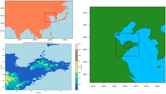
Figure 1.
Diagram of the WRF simulation area. The top-left figure shows the location of the simulated area relative to Asia, inside the red box is the simulation area, the right figure shows the three-layer simulation nested map, and the bottom-left figure shows the elevation map of the d02 area.

Table 1.
Experimental protocol for WRF sensitivity.
To guarantee the accuracy and reliability of the simulation outcomes, a 16 h spin-up is undertaken before the commencement of WRF simulations. This pre-warming phase encompasses the initial 16 h of the WRF simulation and aims to attain model stability. This procedure ensures that the initial conditions for the simulation are physically consistent and mitigates abrupt transitions, thereby minimizing errors and instability throughout the simulation process. Consequently, the time interval considered for the comparative sensitivity experiments in this study spans from 00:00 on 23 September 2017 to 02:00 on 30 September 2017 in Beijing time.
2.2.3. Assessment of Model Performance
This paper assesses the accuracy of wind speed simulation through the utilization of metrics such as the correlation coefficient, bias, root mean square error (RMSE), and mean absolute percentage error (MAPE). The RMSE serves as a robust indicator of the precision of the predicted data sequence. Simultaneously, the MAPE is employed to characterize the extent of error dispersion and mitigate the concern of offsetting biases in sequential data.
The covariance between variables X and Y is denoted as Cov(X, Y), whereas Var[X] and Var[Y] represent the variances of variables X and Y, respectively. In probability theory and statistics, covariance is utilized to quantify the overall deviation between the two variables. Variance, being a specific case of covariance, characterizes situations where the two variables are identical. The formulas for their calculations are as follows:
X is the variable, X1 is the sample mean, n is the sample size, and E represents the expectation.
The sample size is denoted by n, the predicted value of the ith sample by the model is represented by Pi’, and the measured value of the ith sample is indicated by Pi.
The wind direction agreement rate (WDAR) is a widely used metric for assessing the accuracy of wind direction predictions, serving as a meteorological indicator that quantifies the similarity between two wind direction datasets. The calculation involves tallying matching wind direction values in both datasets and dividing that count by the total number of instances to derive the agreement rate. For instance, if both datasets represent wind direction values within the 0 to 360-degree range, agreements are considered for differences less than or equal to 22.5 degrees. The wind direction agreement rate is typically expressed as a percentage and aids in evaluating the similarity between the two wind direction datasets.
2.2.4. WRF Simulation for the Jiaodong Peninsula in 2022
The WRF simulation for the Jiaodong Peninsula region in 2022 was conducted in this study due to the lower sensitivity to temporal and spatial resolutions compared to the sensitivity experiments in the previous section, and a larger simulation domain, a two-layer nesting approach, was employed. The simulation center was located at 36.5° N, 120.4° E, with horizontal grid numbers (resolutions) of 200 × 200 (9 km) and 190 × 190 (3 km) for the outer and inner nests, respectively. Similarly, when simulating the wind energy density distribution in the Jiaodong Peninsula, only the innermost nesting layer (d02) is utilized. Figure 2 displays the land-use types for the second nested layer (d02), with the left image representing the default land-use types in the WRF model and the right image illustrating the land-use types after replacement. Urban areas are highlighted in red. The second nesting layer covered the entire Jiaodong Peninsula and its adjacent waters. The simulation period started from UTC 1 January 2022, 00:00, and ended at UTC 31 December 2022, 18:00, with a 60 min output interval. The initial fields were updated every six hours using GDAS data, with a forecast lead time of six hours and a spatial resolution of 0.25° × 0.25°. The parameterization scheme selected for WRF was the optimal scheme for simulating wind speed chosen in this study. Twelve simulations were conducted to mitigate the impact of accumulated errors on the simulation accuracy, each lasting for one month. Over the past two decades, rapid urbanization has occurred in the Jiaodong Peninsula. The land-use type data for 2022 were utilized in this study. Using the latest land-use type data in WRF simulations is crucial for improving the accuracy of model surface parameterization, thus enhancing the accuracy of simulating meteorological processes and improving the reliability of weather and climate predictions.
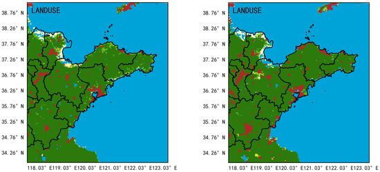
Figure 2.
The land-use types for the second nested layer (d02) are depicted, with the left image representing the default land-use types in the WRF model, and the right image illustrating the land-use types after replacement. In the modified land-use types, urban areas are highlighted in red. Marine areas in blue, non-urbanized areas on land in green.
As a fundamental component of the climate system, the ocean dynamically updates its sea surface temperature (SST) to ensure the model’s alignment with real-world conditions. Throughout the simulation, the SST experiences temporal fluctuations, impacting atmospheric dynamics and thermodynamics, thereby improving the precision and dependability of the simulation outcomes. Therefore, a dynamic SST was employed in this simulation, with SST data sourced from the Global Data Assimilation System (GDAS) reanalysis serving as one of the inputs for establishing the initial conditions in the Weather Research and Forecasting (WRF) model.
2.2.5. Wind Energy Calculation
Wind power density serves as a comprehensive index for assessing the state of wind energy resources in a specific area. It is precisely defined as the wind energy vertically passing through a unit area of airflow within a unit of time. Wind energy is influenced by factors such as the magnitude of wind speed, the frequency distribution of wind speeds, and air density. The following expression represents wind power density:
where n represents the number of records within the designated period, ρ denotes air density, and vi3 represents the cube of the wind speeds recorded for the ith observation. DWP is the wind power density expressed in units of W/m2. The air density (ρ) is measured in units of kg/m3, and its calculation method is as follows:
In the equation, P represents atmospheric pressure, R denotes the gas constant, and T represents the temperature in Kelvin. The value of R used in this paper is 287 J/kg·K.
3. Results
3.1. Atmospheric Circulation Background
Figure 3 and Figure 4 depict images derived from ERA5 reanalysis data. The following weather analysis can be conducted based on the weather patterns and surface wind field changes depicted in Figure 3. From 23 to 30 September 2017, an examination of the 500 hPa geopotential height field reveals fluctuations in the westerly jet stream. Specifically, between the 23rd and 26th, and from the 27th to the 28th, there are two troughs passing through the 500 hPa geopotential height field, while a high-pressure ridge dominates the rest of the time. This variation indicates significant dynamic activity in the atmosphere. Furthermore, by observing the 850 hPa wind field, it is evident that westerly winds prevail during this period. This wind pattern suggests the presence of sustained southwest winds in the lower atmosphere, potentially with significant wind speeds. Such wind field structures are often associated with warm and moist air masses, which could lead to localized precipitation events.
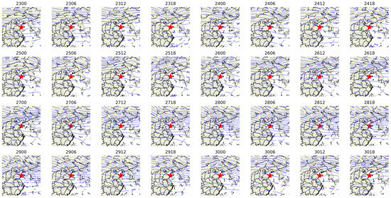
Figure 3.
The 500 hPa geopotential height field superimposed on 850 hPa wind field from 23 to 30 September 2017. The blue lines in the figure represent the 500 hPa geopotential height field, while wind vectors represent the 850 hPa field. The titles above each subplot indicate the date and time. The red pentagram represents the simulation center.

Figure 4.
Temporal variation in latitudinal and longitudinal wind speed in the simulated area from 23 to 30 September 2017. The red pentagon star represents the observation station. Different colored dots represent different times; in general, the lighter the color, the later the time.
Figure 4 presents the temporal variations in meridional and zonal wind speeds. The deepening of the color-coded markers reflects the passage of time. Based on Figure 4, we can discern the changing trends in wind speed. Over the observation period, wind speeds gradually increase from initially lower levels, followed by a gradual decrease. These fluctuations in wind speed may be influenced by atmospheric circulation, such as variations in pressure gradients and interactions between high-pressure and low-pressure systems.
Based on the ERA5 reanalysis data summarized above, we can infer that, during this period, there was significant dynamic activity in the atmosphere, as evidenced by fluctuations in the 500 hPa geopotential height field and the presence of the westerly jet stream. Additionally, the 850 hPa wind field exhibited sustained southwest winds, indicating the presence of warm and moist air masses that could lead to localized precipitation. The changes in surface wind patterns, transitioning from southeast to northerly winds and then back to southeast winds, suggest an evolution in atmospheric circulation. The temporal variations in wind speed showed increasing and decreasing trends, likely influenced by atmospheric circulation and pressure system changes.
3.2. Sensitivity Analysis
3.2.1. Experimental Results of Near-Ground Wind Sensitivity
The observations from Figure 5 reveal that all six boundary-layer parameterization schemes can effectively represent the trends in wind speed variations. Across the entire simulation period, the characteristic pattern of higher daytime wind speeds and lower nighttime wind speeds is evident in all parameterization schemes, and the trends in wind speed changes are consistent across different height levels. Figure 6 illustrates the changes in the cosine of the wind direction at 80 m, revealing a transition from southerly to northerly winds during the simulation period. At the 80 m height level, the wind direction simulated in all parameterization schemes consistently matches the observed wind direction. However, a significant change in wind direction occurs from the afternoon of the 27th to the night of the 28th, which is not well reproduced by most schemes, except for the MRF and BL parameterization schemes. Vertically, the trends in wind speed variations remain consistent across all height levels, indicating that, regardless of the chosen parameterization scheme, vertical wind speed changes exhibit uniformity during the simulation period.
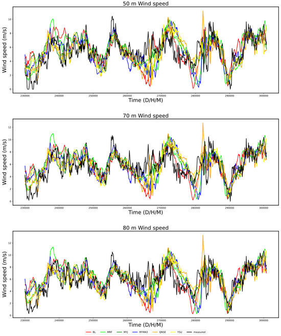
Figure 5.
Comparison of wind speed sensitivity experiments at different heights.
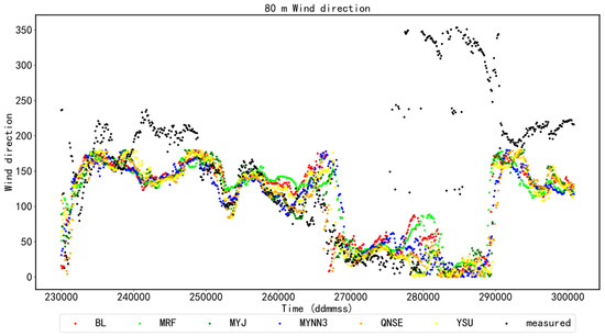
Figure 6.
Comparison of wind sensitivity experiments at 80 m height.
Based on the analysis results of Figure 5 and Figure 6, the six boundary-layer parameterization schemes can effectively simulate the variation trends of wind speed. The differences in wind speed between day and night are accurately represented, and the variation trends of wind speed in the vertical direction are consistent. However, there are certain areas for improvement in simulating wind direction during specific periods, and some parameterization schemes fail to accurately capture the fluctuations in wind direction.
Table 2 presents the sensitivity experiment results at a height of 50 m, comparing the performance of various parameterization schemes using indicators such as the correlation coefficient, root mean square error, bias, and mean error rate. The research results demonstrate that optimal performance is achieved by the YSU parameterization scheme, with root mean square error and bias values recorded at 1.68 and 1.28, respectively. Conversely, the BL parameterization scheme performs the worst, with correlation coefficient, root mean square error, and bias values of 0.55, 1.89, and 1.46, respectively. Although the correlation coefficient of the YSU parameterization scheme is slightly inferior to that of the MRF scheme, its exceptional performance on various other statistical metrics leads us to consider the YSU parameterization scheme as the optimal choice, while the BL needs improvement to enhance its predictive accuracy.
Table 2.
Results of wind field sensitivity experiments at 50 m height. The best results are shown in bold. The same is true for the table below.
Furthermore, the mean error rate is one of the most important indicators for assessing the performance of different parameterization schemes. The mean error rate refers to the mean error ratio to the observed wind speed. The research results demonstrate that the YSU parameterization scheme performs the best in terms of the mean error rate, with a value of 0.27, indicating that YSU can predict wind speed more accurately. In contrast, the BL parameterization scheme performs the worst in terms of the mean error rate, with a value of 0.50, indicating the need for improvement in the BL parameterization scheme to enhance its wind speed prediction accuracy.
Considering all indicators, we recommend using the YSU parameterization scheme when predicting wind speed and wind direction at a height of 50 m, as it exhibits the best performance.
According to Table 3, we can observe variations in the sensitivity performance of different models at a height of 70 m. Firstly, the mean error rate is the most crucial indicator for evaluating wind speed accuracy. We can see that the YSU parameterization scheme performs the best, with a mean error rate of 0.27, while the BL parameterization scheme performs the worst, with a mean error rate of 0.46. This indicates that the YSU parameterization scheme accurately predicts wind speed. Secondly, the correlation coefficient reflects the degree of linear correlation between model predictions and actual observed values. The experimental results show that the MRF parameterization scheme has the highest correlation coefficient, reaching 0.67, whereas the MYNN3 parameterization scheme has the lowest, with a coefficient of only 0.56. This suggests that the MRF parameterization scheme fits actual observed values better and has a closer linear relationship between predictions and observed values. The YSU parameterization scheme demonstrates the best overall performance among all indicators. Therefore, when forecasting wind speed at a height of 70 m, considering using the YSU boundary-layer scheme is advisable.
Table 3.
Results of wind field sensitivity experiments at 70 m height. The best results are shown in bold.
According to the results presented in Table 4, it is evident that, at a height of 80 m, the wind direction prediction accuracy relatively improved for all six parameterization schemes, with all achieving accuracy rates exceeding 55%. Specifically, the QNSE parameterization scheme performs the best, earning a wind direction matching rate of 75.62%. In contrast, the MRF parameterization scheme serves the poorest, with a wind direction matching rate of only 56.97%. The MRF parameterization scheme also exhibits the highest correlation coefficient, reaching 0.68. The YSU parameterization scheme boasts the lowest mean error rate, at 0.27, showcasing the best performance among the six parameterization schemes. Therefore, overall, the YSU parameterization scheme demonstrates relatively favorable performance across all indicators. These results suggest that adopting the YSU parameterization scheme for predicting wind speed and wind direction at an 80 m height.
Table 4.
Results of wind field sensitivity experiments at 80 m height. The best results are shown in bold.
3.2.2. Experimental Results of Near-Formation Atmospheric Pressure Sensitivity
Table 5 displays the evaluation metrics for simulating atmospheric pressure using different parameterization schemes. These evaluation metrics include the correlation coefficient, root mean square error, bias, and mean error rate, which assess the disparities between simulated results and observed values. From the table, it can be observed that different parameterization schemes exhibit variations in the accuracy and reliability of their simulation results. The YSU parameterization scheme performs the best among all evaluation metrics, with the smallest root mean square error, minimal bias, and the lowest mean error rate. In contrast, the BL parameterization scheme exhibits the most significant root mean square error and the highest bias. This indicates that the YSU parameterization scheme offers higher accuracy and reliability in simulating atmospheric pressure, while the performance of the BL parameterization scheme is inferior.
Table 5.
Results of atmospheric pressure sensitivity experiments at 50 m height. The best results are shown in bold.
3.2.3. Experimental Results of Near-Formation Temperature Sensitivity
Table 6 presents the results of sensitivity experiments simulating atmospheric temperature at a height of 50 m using different parameterization schemes. Firstly, across all parameterization schemes, the correlation coefficients range from 0.84 to 0.88, indicating that all schemes possess good predictive capabilities and are relatively stable. The root mean square errors are also relatively small, suggesting that the differences between predicted results and observed values are minimal, with a slight variation in error among different schemes. However, there are some differences among the schemes regarding bias and the mean error rate. Specifically, the MRF parameterization scheme exhibits relatively high bias and mean error rates, implying the potential presence of systematic biases in this scheme. Conversely, the YSU parameterization scheme performs the best in these aspects, indicating its relatively accurate performance in simulating atmospheric temperature at a 50 m height.
Table 6.
Results of temperature sensitivity experiments at 50 m height. The best results are shown in bold.
3.2.4. Experimental Results of Near-Ground Relative Humidity Sensitivity
Table 7 presents the data table of sensitivity experiment results for near-surface relative humidity. From the data table, it can be observed that the MRF scheme achieves the highest correlation coefficient, standing at 0.80. However, the MRF scheme lags behind other models regarding the root mean square error and bias, with values of 20.49 and 17.30, respectively. The QNSE scheme, on the other hand, outperforms all models, with the best root mean square error, bias, and mean error rate. This indicates that the QNSE scheme’s predictions are closer to the actual observed values, with more minor errors. It also suggests that this parameterization scheme accurately predicts near-surface relative humidity.
Table 7.
Results of relative humidity sensitivity experiments at 50 m height. The best results are shown in bold.
3.3. Wind Energy Density and Vertical Profile
3.3.1. Temporal Distribution of Wind Energy Density and Vertical Profile in Jiaodong Peninsula in 2022
The temporal distribution and vertical profiles of wind energy density in the Jiaodong Peninsula in 2022 can be observed based on the data illustrated in Figure 7. The highest wind energy density in the Jiaodong Peninsula occurred from March to May, while the lowest values were recorded from July to August during the same year. This indicates a pronounced seasonal variation in wind energy resources in the Jiaodong Peninsula, with higher densities observed in spring and early summer and relatively lower densities in the summer. Notably, the variations in wind energy density at different heights exhibit a consistent trend. With an increased measuring size, there is a distinct exponential increase in wind energy density. This implies that, as the vertical ascent of the atmospheric layer progresses, the wind speed gradually increases, leading to a corresponding increase in wind energy density.
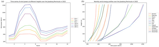
Figure 7.
Time series of wind power at different heights over the Jiaodong Peninsula in 2022 (a) and monthly wind energy profiles over the Jiaodong Peninsula in 2022 (b).
3.3.2. Wind Energy Density Distribution in Jiaodong Peninsula in April and August 2022
Significant seasonal variations in wind energy density were observed in the Jiaodong Peninsula from March to May of the specified year. During this period, the wind energy density in the region reached its annual peak, while a notable decrease was observed from July to August, reaching its annual minimum. Based on these observations, we selected April as a representative month with high wind energy density and August as an expected month with low wind energy density for detailed analysis, as depicted in Figure 8.
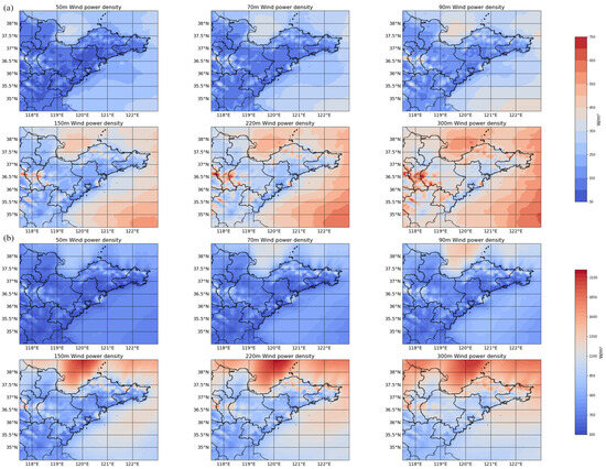
Figure 8.
(a) Distribution of wind energy density by height in the month representing low wind energy density (August), and (b) distribution of wind energy density by height in the month representing high wind energy density (April).
Regarding the distribution of wind energy density on land, it is evident that April is significantly higher than August. Furthermore, the wind energy density across various locations is almost similar in the distributions of other months. Notably, the mountainous areas in central Shandong and the hilly areas south of Yantai and Weihai exhibit higher wind energy density in April, making them regions with relatively abundant wind energy resources on land. Overall, the wind energy density at sea is much higher than on land. However, due to the influence of the monsoon, the wind energy density over the Bohai Sea is significantly higher than that over the Yellow Sea in April, while this trend reverses in August. This suggests that seasonal variations significantly impact the distribution of offshore wind energy.
3.4. WRF-Modelled Wind Energy Density Distribution Compared to ERA5 Reanalysis Data
Figure 9 illustrates the wind energy density distribution calculated using ERA5 reanalysis data at a height of 100 m, where (a) represents April and (b) represents August. Compared to WRF simulations, the wind energy density calculated using ERA5 reanalysis data shows a similar trend at a height of 90 m. However, due to resolution limitations, the ERA5 reanalysis data fail to accurately reflect the finer wind energy density distribution at the 100 m height, particularly evident in the Laizhou Bay and mountainous hilly areas.
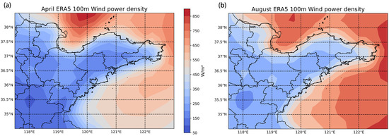
Figure 9.
The 100m wind energy density distribution, simulated using ERA5: (a) April 2022; (b) August 2022.
This limitation emphasizes the importance of choosing appropriate models and data sources in wind energy research to obtain more accurate and reliable results, especially when analyzing complex terrain regions. Future studies may consider further optimizing model parameters and enhancing data resolution to understand wind energy density distribution in different geographical areas.
4. Discussion
Several limitations exist in this study. Firstly, local meteorological features may influence the selection of model parameterization schemes. Hence, its applicability in other regions requires cautious evaluation. Secondly, this study did not consider the potential long-term impact of climate change on wind energy distribution, which is a direction for future in-depth exploration. Additionally, comparing model results with actual measurement data validates the simulation accuracy. However, this study only utilized one site, and subsequent research could involve more observations to identify more accurate parameterization schemes. Future research can further address these limitations to enhance the reliability and applicability of the model. In future investigations, considering more advanced models and data sources and incorporating additional meteorological and geological factors can provide a more comprehensive and accurate depiction of the wind energy resource distribution in the Jiaodong Peninsula and its surrounding areas.
5. Conclusions
In this study, we have investigated the applicability of different boundary-layer and near-surface-layer schemes in simulating the near-surface wind field in the Jiaodong Peninsula. The results indicate that the YSU parameterization scheme performs the best in simulating wind speed at various heights, while the BL parameterization scheme exhibits the poorest performance. The QNSE parameterization scheme performs best in simulating wind direction, whereas the MRF parameterization scheme performs the worst, and YSU is slightly inferior to QNSE. Therefore, using the YSU parameterization scheme for predicting near-surface wind speed and the QNSE parameterization scheme for predicting near-surface wind direction is recommended. The YSU parameterization scheme performs best in simulating atmospheric pressure and temperature at a 50 m height, while the MRF and BL parameterization schemes perform poorly. The evaluation metrics for the MYJ, QNSE, and YSU parameterization schemes are relatively close to YSU, but still slightly worse. In the near-surface relative humidity sensitivity experiment, all parameterization schemes exhibit significant errors, with the MRF parameterization scheme having the highest correlation coefficient. However, the QNSE parameterization scheme has the optimal root mean square error, bias, and mean absolute error among all models, indicating its high accuracy in predicting near-surface relative humidity.
Following this, we utilized the YSU boundary-layer scheme along with the land-use type data for the year 2022 provided by the Terra and Aqua combined Moderate Resolution Imaging Spectroradiometer (MODIS) Land Cover Type (MCD12Q1) Version 6.1 data product to simulate the wind energy density distribution in the coastal hilly areas of the Jiaodong Peninsula in 2022. The results reveal a significant seasonal variation in wind energy density in the Jiaodong Peninsula. March to May exhibit the highest wind energy density, while July to August show the lowest, indicating a higher wind energy density in spring and early summer and relatively lower density in summer. At different elevations, wind energy density exhibits exponential growth with the increase in measurement height. On land, the central mountainous region of Shandong, Yantai, and the southern hilly areas of Weihai have greater wind energy density than other locations. Overall, offshore wind energy density surpasses that on land but is significantly influenced by monsoons. In April, the wind energy density over the Bohai Sea is higher than that over the Yellow Sea, with this trend reversing in August.
Subsequently, we compared the wind speed predictions at an 80 m height from GFS, GDAS reanalysis data, and WRF. The results indicate that WRF’s predictions are significantly superior to GFS and GDAS. When using the optimal YSU parameterization scheme to predict wind speed, WRF shows a notable improvement in various evaluation metrics compared to GFS and GDAS. In terms of wind power prediction, WRF’s forecasts perform better. Therefore, overall, the WRF model demonstrates greater accuracy and reliability in predicting wind speed and power.
Following this, a comparison was made between the wind energy density distribution simulated by WRF and the results from ERA5 reanalysis data. Although the two maintain consistent trends, the WRF simulation exhibits finer features, mainly showcasing outstanding performance in mountainous hilly areas. This difference may arise from WRF’s ability to accurately capture terrain complexity and local meteorological features, providing more detailed information on wind energy density distribution. This observation underscores the crucial role of model selection and data sources in wind energy research, especially in scenarios where a high spatial resolution is needed to reveal geographical complexities. Future research directions may consider further refining the parameter configuration of WRF simulations to optimize its performance under different topographic conditions, thereby gaining a more comprehensive understanding of the spatial distribution of wind energy resources.
Author Contributions
Conceptualization, Y.S.; methodology, Y.S., S.H. and Z.L.; software, Y.S. and Z.Z.; validation, L.W. and Z.G.; formal analysis, S.H.; investigation, Y.S. and Y.Y.; resources, Y.S. and Y.Y.; data curation, Y.S. and Y.Y.; writing—original draft preparation, Y.S.; writing—review and editing, S.H. and Z.L.; visualization, Y.S. and Z.G.; supervision, Y.S.; project administration, Y.S., S.H. and Z.L.; funding acquisition, Z.G. All authors have read and agreed to the published version of the manuscript.
Funding
This work was funded by the National Natural Science Foundation of China (grant no. 42175082).
Data Availability Statement
Publicly available datasets were analyzed in this study. GFS and GDAS data are available at https://www2.mmm.ucar.edu/wrf/users/download/free_data.html (accessed on 23 July 2023). ERA5 data are available at https://cds.climate.copernicus.eu/cdsapp#!/home (accessed on 23 July 2023). MODIS data are available at https://lpdaac.usgs.gov/products/mcd12q1v061/ (accessed on 23 July 2023).
Acknowledgments
The authors express their gratitude to Bingcheng Wan and Zexia Duan for their valuable assistance and insightful discussions related to the illustrations in this article.
Conflicts of Interest
Yunhai Song, Sen He, Zhenzhen Zhou, Liwei Wang and Yufeng Yang are employees of China Southern Power Grid Co., Ltd. Ultra High Voltage Transmission Company, Electric Power Research Institute. The paper reflects the views of the scientists and not the company. The authors declare no conflicts of interest.
References
- Amjad, M.; Zafar, Q.; Khan, F.; Sheikh, M. Evaluation of weather research and forecasting model for the assessment of wind resource over Gharo, Pakistan. Int. J. Climatol. 2015, 35, 8. [Google Scholar] [CrossRef]
- Salvação, N.; Soares, C.G.; Bentamy, A. Offshore Wind Energy Assessment for the Iberian Coasts Using Remotely Sensed Data; Taylor & Francis Group: Didecott, UK, 2015. [Google Scholar]
- Theodore, M.G.; Dimitrios, M.; Ioannis, Z. Performance evaluation of the Weather Research and Forecasting (WRF) model for assessing wind resource in Greece. Renew. Energy 2017, 102, 190–198. [Google Scholar] [CrossRef]
- Li, Z.; Wan, B.; Duan, Z.; He, Y.; Yu, Y.; Chen, H. Evaluation of HY-2C and CFOSAT Satellite Retrieval Offshore Wind Energy Using Weather Research and Forecasting (WRF) Simulations. Remote Sens. 2023, 15, 4172. [Google Scholar] [CrossRef]
- Wang, J.; Wang, H.J. Forecasting of Wind Speed in Rudong, Jiangsu Province, by the WRF Model. Clim. Environ. Res. 2013, 18, 145–155. [Google Scholar]
- Storm, B.; Dudhia, J.; Basu, S.; Swift, A.; Giammanco, I. Evaluation of the Weather Research and Forecasting model on forecasting low-level jets: Implications for wind energy. Wind. Energy 2009, 12, 81–90. [Google Scholar] [CrossRef]
- Shin, H.H.; Hong, S.-Y. Intercomparison of Planetary Boundary-Layer Parametrizations in the WRF Model for a Single Day from CASES-99. Bound. -Layer Meteorol. 2011, 139, 261–281. [Google Scholar] [CrossRef]
- Deppe, A.J.; Gallus, W.A.; Takle, E.S. A WRF Ensemble for Improved Wind Speed Forecasts at Turbine Height. Weather Forecast. 2013, 28, 212–228. [Google Scholar] [CrossRef]
- Draxl, C.; Hahmann, A.N.; Peña, A.; Giebel, G. Evaluating winds and vertical wind shear from Weather Research and Forecasting model forecasts using seven planetary boundary layer schemes. Wind. Energy 2014, 17, 39–55. [Google Scholar] [CrossRef]
- Carvalho, D.; Rocha, A.; Gómez-Gesteira, M.; Santos, C.S. Sensitivity of the WRF model wind simulation and wind energy production estimates to planetary boundary layer parameterizations for onshore and offshore areas in the Iberian Peninsula. Appl. Energy 2014, 135, 234–246. [Google Scholar] [CrossRef]
- Ramos, D.; Da Fonseca Lyra, R.; Júnior, R. Previsão do vento utilizando o modelo atmosférico WRF para o estado de Alagoas. Rev. Bras. De Meteorol. 2013, 28, 163–172. [Google Scholar] [CrossRef]
- Tuchtenhagen, P.; Martins Basso, J.; Yamasaki, Y. AvaliaÇÃo Do Potencial EÓlico No Brasil Em 2011. Ciência E Nat. 2014, 36, 390–401. [Google Scholar] [CrossRef]
- García-Díez, M.; Fernández, J.; Fita, L.; Yagüe, C. Seasonal dependence of WRF model biases and sensitivity to PBL schemes over Europe. Q. J. R. Meteorol. Soc. 2013, 139, 501–514. [Google Scholar] [CrossRef]
- Liu, X.; Lai, X.; Chen, L. Effect of parameterization of atmospheric model physical process on wind speed prediction in wind farm. Water Resour. Power 2012, 30, 208–210+145. [Google Scholar]
- Li, X.M.; Shang, X.B.; Chen, L.; Zhang, J.; Liu, X. Simulation of wind speed under different terrain conditions based on WRF model. Hydropower New Energy 2019, 33, 60–64. [Google Scholar]
- Salvação, N.; Soares, C.G. Wind resource assessment offshore the Atlantic Iberian coast with the WRF model. Energy 2018, 145, 276–287. [Google Scholar] [CrossRef]
- Huidong, L.; Björn, C.; Lichuan, W.; Christoffer, H.; Heiner, K.; Stefan, I.; Erik, S. A sensitivity study of the WRF model in offshore wind modeling over the Baltic Sea. Geosci. Front. 2021, 12, 101229. [Google Scholar] [CrossRef]
- Caralis, G.; Gao, Z.; Yang, P.; Huang, M.; Zervos, A.; Rados, K. Development of Aeolian Map of China Using Mesoscale Atmospheric Modelling. Renew. Energy 2015, 74, 60–69. [Google Scholar] [CrossRef]
- Research Data Archive. NCAR RDA Dataset Ds083.2. Available online: http://rda.ucar.edu/datasets/ds083.2/ (accessed on 23 July 2023).
- Research Data Archive. NCAR RDA Dataset Ds083.3. Available online: http://rda.ucar.edu/datasets/ds083.3/ (accessed on 23 July 2023).
- Copernicus Climate Data Store. Copernicus Climate Data Store. Available online: https://cds.climate.copernicus.eu/cdsapp#!/dataset/reanalysis-era5-single-levels?tab=overview (accessed on 23 June 2023).
- LP DAAC—MCD12Q1—USGS. Available online: https://lpdaac.usgs.gov/products/mcd12q1v061/ (accessed on 12 November 2023).
Disclaimer/Publisher’s Note: The statements, opinions and data contained in all publications are solely those of the individual author(s) and contributor(s) and not of MDPI and/or the editor(s). MDPI and/or the editor(s) disclaim responsibility for any injury to people or property resulting from any ideas, methods, instructions or products referred to in the content. |
© 2024 by the authors. Licensee MDPI, Basel, Switzerland. This article is an open access article distributed under the terms and conditions of the Creative Commons Attribution (CC BY) license (https://creativecommons.org/licenses/by/4.0/).