Standardized Precipitation and Evapotranspiration Index Approach for Drought Assessment in Slovakia—Statistical Evaluation of Different Calculations

Abstract

In the conditions of rising air temperature and changing precipitation regimes in Central Europe and Slovakia over the last two decades, it is necessary to analyse drought, develop high-quality tools for drought detection, and understand its reactions to the emerging drought situation. One of the frequently used meteorological drought indices is the Standardized Precipitation and Evapotranspiration Index (SPEI). Several parameters can be modified in different steps of the calculation process of SPEI. In the article, we analyse the influence of selected adjustable parameters on the index results. Our research has shown that the choice of a statistical distribution (Log-logistic, Pearson III, or Generalized Extreme Value) for fitting water balance can affect the feasibility of calculating distribution parameters (and thus the index) from the provided input data, as well as lead to either underestimation or overestimation of the index. The normality test of SPEI can be used as a tool for the detection and elimination of highly skewed indices and cases when the indices were not well determined by the distribution function. This study demonstrated improved results when using the GEV distribution, despite the common use of the Log-logistic distribution. With the Pearson III distribution, unusually high or low SPEI values (|SPEI| > 6) were detected.

1. Introduction

In the last two decades, a significant change in the temporal and spatial distribution of precipitation occurred in Central Europe, including Slovakia. Precipitation in the warm half-year is more often in the form of short and intensive showers rather than long-lasting stratiform precipitation. At the same time, in the cold half-year, there is a decrease in snow cover totals and the number of days with snow cover (except in high mountain locations) [1,2]. Although the annual sum of precipitation totals in Slovakia did not change significantly, more often and longer rainless periods in the conditions of warming climate lead to more frequent and extensive soil drought (especially in the warm half-year and in the lowlands of the country) [2,3,4]. Air temperature and evapotranspiration are other crucial factors that mainly affect drought intensity. Prolonged droughts occur when large-scale anomalies in atmospheric circulation persist for months or seasons [5]. Several authors [6,7,8] emphasize the necessity of studying the effect of climate warming on the occurrence and intensity of drought. According to climate models, an increase in drought and prolonged dry spells combined with high temperatures are expected in many regions of Europe, including Slovakia [9,10].

Increasing aridity affects multiple ecosystems in the studied region. In forestry, a decrease in growth or even mortality of some species has been recorded due to drought. Drought also creates suitable conditions for the increased occurrence of certain pests and diseases, such as bark beetles and wood-decay fungus. It can also lead to shifts in the ranges of specific tree species toward higher altitudes or the replacement of less adaptable species with more resilient ones [11,12]. Grasslands, which can act as hotspots of biodiversity in landscapes dominated by agriculture, are also one of the ecosystems threatened by drought. Within pastures, we can observe shifts in grassland composition toward more drought-tolerant species. At the same time, drier conditions can elevate the risk of igniting and spreading fires [13]. The crop system is often the first sector to be affected by the onset of drought. In addition to vegetation stress due to reduced water availability and disruption in food security, drought can also negatively impact plant heights and biomass yields (silage production). Therefore, insufficient fodder supply to the livestock sector due to high water stress during the production season can lead to substantially lower milk production [14].

To better understand drought and the responses of ecosystems to drought, it is necessary to analyse and understand the weaknesses and strengths of drought indicators. This work focuses on one of the most widely used meteorological drought indices—the Standardized Precipitation Evapotranspiration Index (SPEI). We will analyse the suitability of some frequently used methods for calculating this index based on data from Slovakia.

SPEI was originally proposed by Vicente-Serrano, Beguería, and López-Moreno [6] as an upgrade to the widely used Standardized Precipitation Index (SPI) [15]. The only input parameter for SPI is the precipitation sum for a studied period. The upgraded index, SPEI, is based on the climatic water balance (D)—the difference between precipitation and potential evapotranspiration instead of precipitation only. This improvement brought other meteorological variables like temperature, wind, or humidity into the drought estimation. Using precipitation alone does not describe all factors that influence drought (especially agricultural drought and drought in summer) [16,17,18].

The first step in SPEI calculation is choosing a suitable method for potential evapotranspiration (PET) assessment. When defining the index, the authors of the SPEI recommended a simple Thornthwaite method to calculate PET [6]. This method requires only the air temperature and latitude of the station. After further analysis, the authors prioritized the more complex Penman–Monteith (P.M.) method [7]. P.M. is also recommended by the Food and Agricultural Organization (FAO) as the standard method for PET assessment based on meteorological data [19]. Except for air temperature, P.M. requires wind speed, relative humidity, and solar radiation that are not measured on some meteorological stations resp. are measured with insufficient accuracy. For this reason, the authors of SPEI recommended using the Hargreaves method. The Hargreaves equation only requires daily maximum and minimum temperatures, while the results are very similar to P.M. in monthly and annual timescales [20].

In the next step, the differences between precipitation and PET for the selected reference period are fitted to a suitable probability distribution to transform the original values into standardized units comparable in time and at different time scales. Choosing an appropriate probability distribution for D is a key decision in calculating these drought indices, as selecting an inappropriate distribution can impart bias to the index values, exaggerating or minimizing drought severity [21,22]. The authors of SPEI recommended using the three-parameter Log-logistic distribution [6,23], while they also analysed the suitability of other distributions. The difference between the two commonly used statistical distributions, the GEV and the Log-logistic cumulative probability distribution, is low over most of the range of the variable based on the author’s findings. The relevant differences to discern between the distributions only correspond to less than 2–3% of the data located in the upper and lower tails of the distribution. When they focused only on tails of distributions, there were much higher (less realistic) return periods and more extreme SPEI values for the same D values with the GEV compared to the Log-logistic, both for high and low D values [23]. Therefore, the better fit of extremes is one of the main arguments in favour of Log-logistic distribution, according to the authors of the SPEI. On the other hand, after a couple of goodness of fit tests of D and comparison of discussed distributions (Log-logistic and GEV) directly to the baseline Gaussian distribution, Stagge et al. concluded that the Log-logistic distribution underestimates the extremes and that the GEV distribution is significantly more accurate across the range of typical SPEI values [−2, 2] [24]. Therefore, they suggest using GEV, and when it comes to extremes, they recommend placing reasonable limits on the SPEI time series (e.g., −3 and 3). When there is a reference period of 30 years used for distribution determination, it is impossible to accurately quantify such an extreme event that happened once in hundreds of years (SPEI greater than 3 and less than −3 should occur once in 741 years). It can only be said that it is an extreme event [22].

Among the other authors who focused their studies on SPEI in the conditions of European climate, [25] (Serbia) and [26] (Europe) decided to use GEV in their work, while [27] (Czech Republic); [17] (Europe); [28] (Europe); [29] (six European sites located in mid-latitudes); and [30] (Europe) followed the Log-logistic distribution.

Another methodological inconsistency lies in the method in which the chosen distribution’s parameters are estimated. In the original formulation of the SPEI, the authors recommended using the plotting-position Probability Weighted Moment (ppPWM) method for parameter estimation [6]. Subsequently, unbiased Probability Weighted Moment (ubPWM) and the maximum likelihood method (MLE, a more time-consuming method that requires initial values of the parameters) were suggested as better alternatives [7]. It was shown that using the MLE method to fit parameters for GEV distribution will produce less extreme values of SPEI compared to the PWM method [23]. At the same time, when the GEV distribution is fitted by the MLE method, an important proportion of months with no solution was found [23]. Namely, D values should be bounded by the parameters of the distributions. When the D value is out of these boundaries, the no-solution cases originate due to the irrelevancy of calculated values of parameters. A failure to fit the parameters for a specific month/day leads to missing SPEI values not only in one year but for the particular month/day throughout the entire time series. The no-solution cases were found using PWM as well as using the MLE method for fitting all three studied distributions: Log-logistic, GEV, and Pearson III distribution, but with the MLE method, the number of these cases was higher (especially in the case of GEV) [23]. Therefore, the authors of SPEI [23] prefer the unbiased sample PWM method rather than the MLE method. On the other hand, Stagge et al. [24] recommend using PWMs for initial values and MLE for the final fit. This approach affords the advantages of both methods: speed and stability from PWM and accuracy from MLE. At the same time, the authors experience no fitting failures using this method for both the Log-logistic and the GEV distributions [24].

After fitting D to a suitable distribution, the final values of SPEI are obtained by transforming the cumulative probability density function of D into the standard normal distribution with a mean of 0 and standard deviation of 1. Therefore, the final index is standardized with positive values representing wet and negative dry conditions (

Table 1. Classification of SPEI.

Moisture Category	SPEI
Extremely wet	≥2
Very wet	1.50 to 1.99
Moderately wet	1.00 to 1.49
Near normal	−0.99 to 0.99
Moderately dry	−1.00 to −1.49
Severely dry	−1.50 to −1.99
Extremely dry	≤−2

).

The strengths of SPEI lie in its simple calculation, the sensitivity of the Palmer Drought Severity Index (PDSI) in measuring evapotranspiration demand (caused by fluctuations and trends in climatic variables other than precipitation), and its multi-temporal character [7]. On the other hand, a weakness of the index can be attributed to the inconsistency in its calculation methodology.

Due to the topicality of the drought issue and the flexibility of calculating the Standardized Precipitation Evapotranspiration Index (SPEI) via various parameter choices, potentially leading to different outcomes, our goal in this study is to demonstrate the effectiveness of different approaches and calculation methodologies for SPEI. Specifically, we will analyse the suitability of three commonly used statistical distributions of water balance for SPEI: the Log-logistic, Generalized Extreme Value (GEV), and Pearson III distributions. This analysis aims to shed light on how these choices impact the index based on data from Slovakia. We would like to understand to what extent the choice of statistical distribution affects the final value of the index and whether there are any advantages or disadvantages of the index when using different statistical distributions.

It is worth noting that many analyses utilizing SPEI often default to using the Log-logistic distribution, and sometimes, the specific statistical distribution used is not even mentioned. (Similarly, the methodology for calculating Potential Evapotranspiration (PET) or the choice of the reference period for computing the indices is frequently unspecified.) Therefore, alongside evaluating the appropriateness of the three studied statistical distributions based on data from Slovakia, we also seek to raise the question of how parameter choices can influence the index, particularly in extreme conditions.

We hope this work can serve as a valuable reference for researchers and practitioners involved in drought monitoring who wish to understand better the implications of their parameter choices in SPEI calculations.

2. Materials and Methods

2.1. Study Area

Slovakia is a landlocked Central European country with a temperate climate. It lies approximately between 47° and 50° N and 16° and 23° E (Figure 1). Due to its complex orography, there can be different climate conditions within a small area. The middle of the country and northern areas are mainly mountainous (the Carpathian Mountains) with the highest peak, Gerlachovský štít (2654 m.a.s.l.), and the coldest place in the country according to the average annual air temperature, Lomnický štít −2.9 °C (for the period 1990–2019) [31]. The southern, southeast, and southwest of the country belong to the Pannonian Basin, with the Danubian Lowland in the southwest of the country and the East Slovakian Lowland in the southeast. One of the warmest stations, Hurbanovo, with an average annual air temperature of 11.1 °C in the period 1990–2019, is located on the Danubian Lowland [31]. Danubian Lowland and East Slovakian Lowland represent the most important regions for agriculture in Slovakia. At the same, these lowlands are localities where the warming trend is the most obvious in Slovakia (especially when we speak about warm half-year and summer temperatures). In Hurbanovo, the mean annual temperature in the normal period 1991–2020 was 1.2 °C warmer than in 1961–1990. Mean annual precipitation totals are from 500 mm in the Danubian Lowland to more than 1600 mm in the highest altitudes of the Tatra Mountains and the Low Tatra Mountains. In the lowlands’ hydrology cycle, most precipitation evaporates, while runoff prevails over evapotranspiration in the mountain region. Typically, the driest months are the first three months of the year, while the highest precipitation totals occur during the summer [31,32].

Table 2. List of the stations used in our research; altitude, average monthly maximal air temperature in January (Tmax Jan.) and July (Tmax July); average monthly minimal air temperature in January (Tmin Jan.) and July (Tmin July); average precipitation totals for warm half-year (April-September) (R why); and average sum of potential evapotranspiration for warm half-year (PET why) over the studied period (1981–2019).

	Station	Altitude [m]	Tmax Jan. [°C]	Tmax July [°C]	Tmin Jan. [°C]	Tmin July [°C]	R Why [mm]	PET Why [mm]
1	Báhoň	159	2.55	27.75	−3.25	15.46	307.95	754.21
2	Beluša	248	1.62	26.38	−4.97	13.03	408.28	758.44
3	Bodorová	485	1.03	24.89	−5.69	12.28	343.98	708.09
4	Haniska	200	0.68	26.28	−5.15	14.38	407.84	717.32
5	Jakubovany	385	−0.12	25.14	−5.94	12.69	441.51	703.82
6	Michalovce	123	0.81	27.00	−4.50	15.04	389.48	730.78
7	Spišská Belá	628	−0.05	23.35	−8.30	10.70	456.84	678.71
8	Spišské Vlachy	430	0.37	25.31	−8.17	11.52	470.63	763.28
9	Veľké Ripňany	188	1.97	27.27	−4.56	13.47	317.03	801.01
10	Veľký Meder	112	2.86	27.75	−3.22	14.83	313.82	786.23
11	Vígľaš	340	1.09	26.19	−6.96	11.50	394.04	802.74
12	Vranov nad Topľou	164	0.73	26.86	−4.73	14.29	426.92	749.29
13	Želiezovce	130	2.25	28.21	−4.42	14.40	329.45	824.76

shows the long-term (1981–2019) averages of meteorological data for each station used in this study. The locations of the stations on the map of Slovakia are shown in Figure 1.

2.2. Data

The daily data of air temperature, precipitation sum, wind speed, cloudiness, air humidity, and water vapour pressure (variables required for PET and SPEI calculation) in the period from 1 January 1981 to 31 December 2019 at selected stations (Figure 1) were provided by the Slovak Hydrometeorological Institute.

2.3. Methodology of SPEI Calculation

In our study, two methods of potential evapotranspiration calculation were used: a more complex Penman–Monteith method (P.M.) and a simpler Hargreaves method (Harg.) (modified version with precipitation included) that were recommended as standard methods for PET assessment by the Food and Agricultural Organization [19,20], as well as by the authors of SPEI [7].

The 30-, 92-, and 183-day accumulation periods of climatic water balance D (as an analogy for 1-, 3-, and 6-month periods) were used. The sums of D were calculated on a daily basis and retrograde, i.e., the 30-day sum corresponding to 30 January represents the 30-day sum from 1 January to 30 January, the 31 January belongs to the sum from 2 January to 31 January, etc. The probability distributions of D were then fitted for every day in a year (365 probability distributions for each index length, 29 Februarys were excluded to maintain uniformity of the data in different years). The main advantage of this method (using daily instead of monthly time steps) is a larger statistical sample, but also more detail and a smoother transition of the index.

This study compares three different probability density functions for D: Log-logistic distribution, GEV, and Pearson III distribution. Parameters of distributions were fitted using the MLE method. The MLE method requires initial values of parameters, which were obtained by Unbiased Sample L-moments. According to [18], this parameter fitting method combines the flexibility of the MLE method with the robustness of L-moments.

As for the reference period of the index, we chose a 39-year period from 1981 to 2019, which encompasses the entire study period. We also tested shorter reference periods of 30 and 20 years, but they proved insufficient or less accurate for our purpose. Specifically, when the 20-year reference period was used, a significant portion of the indices (in some cases 30–50%) were not normally distributed (as expected by criteria of goodness of SPEI fit, see [22]), and approximately 0.5% of indices exhibited unlikely extreme values (|SPEI| > 6). This indicates that the 20-year reference period is too short to adequately capture the statistics of the water balance. Moreover, reducing the reference period to 20 years resulted in an increased number of “no-solution” cases, where the model was unable to calculate distribution parameters. The 30-year reference period showed lower percentages of unlikely extremes (|SPEI| > 6) at 0.08%, fewer non-normally distributed indices (approximately 6%), and fewer “no-solution” cases (only a few cases). This implies that a 20-year period is only applicable with significant limitations. However, a 30-year period exhibits better characteristics regarding the distribution of extreme values. With the extension of the reference period, we observed further substantial improvements. Therefore, this study primarily focused on a 39-year reference period.

The entire SPEI calculation process (including fitting parameters for probability density functions) was made with the “SCI” package in the R-programming language [33].

Table 3. Abbreviations for modifications of SPEI used in our study. Modifications are based on the combination of two factors: the PET method (Hargreaves and Penman–Monteith) and the distribution (probability density function) of D (Log-logistic, Pearson III, and GEV). The first letter of the abbreviation is related to the PET method, while the second is to the distribution.

	Potential Evapotranspiration
Distribution	Hargreaves	Penman–Monteith
Log-logistic	hl	pl
Pearson III	hp	pp
Generalized extreme value	hg	pg

shows the abbreviations for SPEI modifications used in our study.

2.4. Choice of the Optimal Probability Density Function of D

Before we analysed the individual statistical distributions, we wanted to know how the index would change if the studied parameter-statistical distribution was changed. We analysed absolute differences between the pairs of indices that differ only in used statistical distribution of water balance. Since we studied three statistical distributions (Log-logistic, GEV, and Pearson III), we had three different pairs of indices. So, for every pair of indices, we had approximately 14,200 (≈365 days × 39 years) differences for each of the two PET methods (P.M. and Harg.) at every station and for all three studied index lengths (1, 3, and 6 months). In this way, we obtained approximately 1,100,000 absolute differences for every pair of indices from which we subsequently calculated the average absolute difference and percentage of absolute differences greater than 0.5 and 2.

In the next part, the suitability of probability density functions was assessed according to three criteria:

• Normality of final SPEI index;
• The number of cases when distribution parameter fitting failed (the number of no-solution cases);
• The number of SPEI extremes.

In the first step, we count events with missing index due to the inability to fit parameters of distribution (since it has been found that the number of these no-solution cases may be related to the choice of the distribution). We compare the number of no-solution cases for three studied distributions.

In the next step, we used the Shapiro–Wilk (S-W) normality test to check the normality of the calculated SPEI, whereas refs. [22,34] showed that the results of this normality test effectively differentiate among the candidate distributions, producing similar results as if we used more complex tests of goodness of fit of D: the Kolmogorov–Smirnov and Anderson–Darling test. At the same, the S-W normality test is recommended for small sample sizes with less than 50 samples. In our study, we tested 365 time series with 39 samples corresponding to 365 values for a given index in a year and 39 years of the study period (1981–2019).

We also focused on extremes and counted the cases when the index was less than −2 and greater than 2, respectively, to find out the ability of the given distribution function to capture extremes. There is a suspicion that statistical distributions lead to a certain number of improbable extremes (for example, a larger number of events found beyond the 6σ range of the distribution).

3. Results and Discussion

3.1. The Influence of Modification of Statistical Distribution on the Final SPEI Value

Before we analyse the advantages and disadvantages of individual statistical distributions, it is appropriate to ask how the change in statistical distribution will influence the final value of an index.

When we compared indices with different statistical distributions, the absolute difference was, on average, 0.047. The smallest difference (<0.04 on average) was observed between indices with Pearson III and GEV distribution, while differences between indices with Pearson III and Log-logistic and GEV and Log-logistic were, on average, lower than 0.055. For each pair, there were few cases when the difference between indices was higher than 0.5 (according to SPEI definition, 0.5 is the threshold for another drought category). However, the percentage of such cases was less than 0.4%. A difference greater than 2 occurred in very rare cases when we compared indices with Log-logistic and Pearson III distributions and indices with GEV and Pearson III distributions. When comparing indices with Log-logistic and GEV distributions, the absolute differences were at most 1 (Figure 2).

3.2. Choice of the Optimal Probability Density Function of D

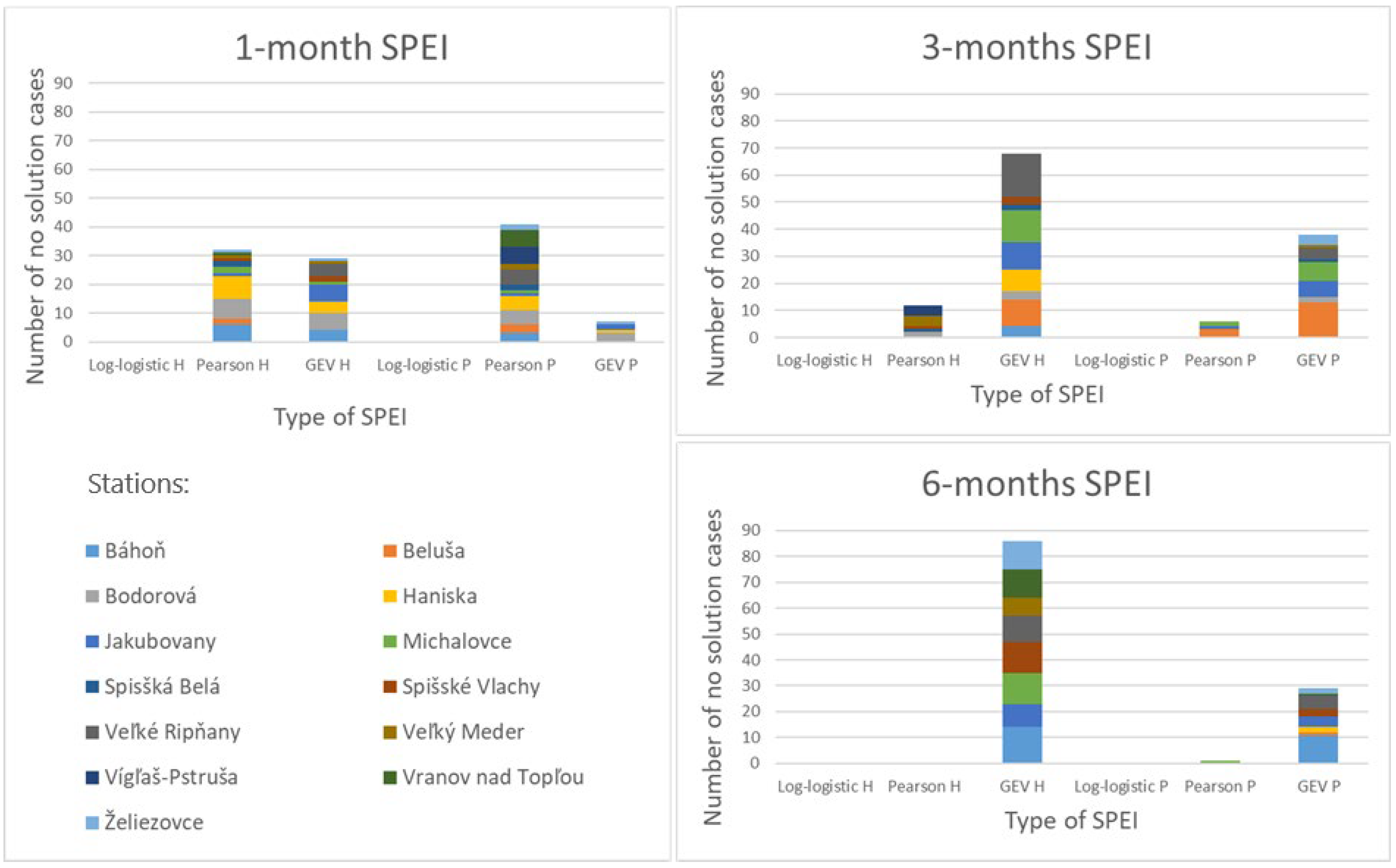
3.2.1. The Number of No-Solution Cases for Parameter Fitting

As we mentioned in Materials and Methods, the “SCI” R package was used for SPEI calculation. This package uses the “mledist” function for parameter fitting. Inside “mledist”, parameters are optimized based on the Nelder–Mead algorithm [35] within the “optim” function. Under certain conditions, given input parameters (initial values of distribution parameters) lead to the degeneracy of the used Nelder–Mead simplex, resp. the distribution parameters cannot be calculated. Under these circumstances, when we do not know the distribution parameters for a certain day, we cannot calculate SPEI for that day along the entire studied period (39-year period). Henceforth, we will call such a case a “no-solution case”. Since we have 365 distributions for each station and each method of SPEI calculation (a combination of PET selection, statistical distribution of water balance, and index length), the maximum number of no-solution cases for a specific station and index type is 365.

The number of no-solution cases can depend on different factors including used distribution, method of PET calculation, length of the index, reference period of the index, and station (Figure 3).

When we focused on the influence of different statistical distributions, the Log-logistic distribution showed the lowest number of no-solution cases based on our results (

Table 4. Number of missing indices due to the inability to fit the distribution parameters. The full sample of indices with the given distribution consists of 1,110,330 indices (3 lengths of the index, 2 different PET methods, 13 stations, and 14,235 days (39 years)).

Distribution	Number of Missing Indices Caused by Parameters Fitting Issues	Percent [%]
Log-logistic	0	0.00
Pearson III	3588	0.32
Generalized extreme value	10,023	0.90

). There were no no-solution cases in the 30- and 39-year reference periods. For a shorter 20-year reference period, there were a maximum of five no-solution cases for one station (at most stations, these cases did not occur). On the other hand, most no-solution cases were found when using GEV distribution, especially in combination with the Hargreaves method of PET calculation.

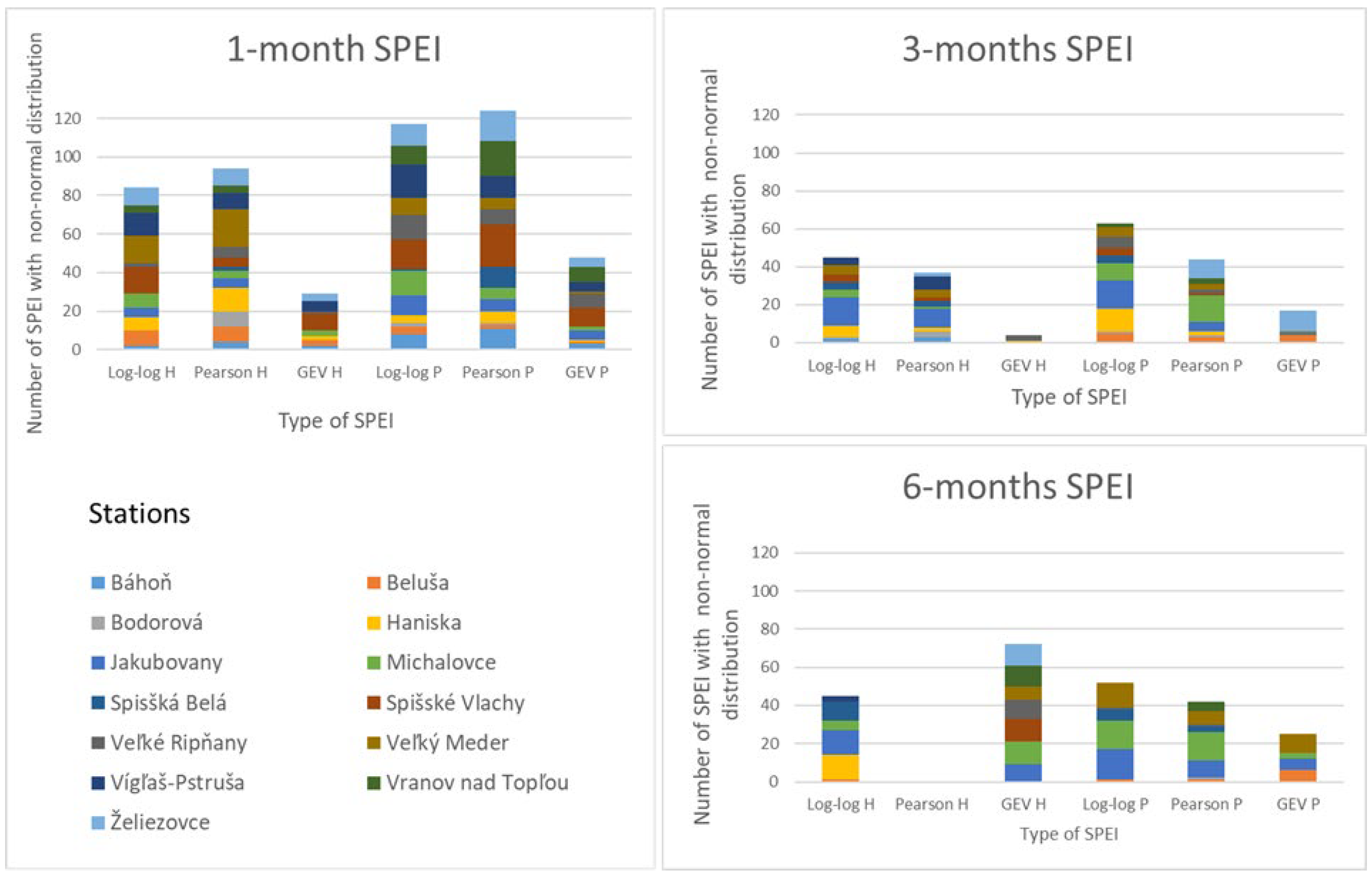
3.2.2. Shapiro–Wilk (S-W) Normality Test of the Final SPEI Index

In cases where it was possible to calculate the parameters of the distribution and thus the SPEI indices, the indices were subsequently tested for normal distribution. Namely, if the selected statistical distribution fits well with the climatic water balance (D), the final values of SPEI should have a normal distribution.

From the view of our experiments of the S-W normality test, the GEV distribution had the lowest number of cases with SPEI not normally distributed and, therefore, the best result (

Table 5. Number and percentage of indices that do not meet the assumption of normality. The full sample of indices depends on the selected distribution and consists of max. 1,110,330 indices (3 lengths of the index, 2 different PET methods, 13 stations, and 14,235 days (39 years)) minus the number of no-solution cases.

Distribution	Number of Missing Indices Caused by Non-Normal Distribution	Percent [%]
Log-logistic	15,834	1.43
Pearson III	14,664	1.32
Generalized extreme value	5070	0.46

). The same results were found for both used PET methods, and all three used lengths of the index, 1, 3, and 6 months (Figure 4). With the GEV distribution, 0.08% to 0.61% of the indices did not follow a normal distribution when using the Hargreaves method for PET calculation, and 0.36% to 1.01% did not follow a normal distribution when using the P.M. method for PET calculation. When we focus on the 1-month index, the second place took Log-logistic distribution (1.77% with PET = Harg and 2.47% with PET = P.-M.), and the third place took Pearson III distribution (1.99% with PET = Harg and 2.64% with PET = P.-M.). In the case of the 3-month and the 6-month index, the second-best distribution was Pearson III distribution (0.74–0.78% with PET = Harg and 0.83–0.89% with PET = P.-M.) and the most inappropriate distribution from the three studied distributions was Log-logistic (0.95% with PET = Harg and 1.10–1.33% with PET = P.-M.).

3.2.3. The Number of SPEI Extremes

After excluding indices when parameters of the distribution cannot be calculated (part 1) and the indices that do not meet the normality assumption (part 2), we found that the number of SPEI extremes does not deviate from the norm. In the case of Log-logistic distribution, 1.15% of indices were greater than 2, and 1.53% were less than −2. When Pearson III and GEV were used, 2.00% and 2.40% of indices were above 2, while 2.59% and 2.00% of cases were below −2 (Figure 5). According to the definition of a standardized normal distribution, 95.4% of data lies between −2 and 2. Therefore, about 2.3% of data is above resp. below the threshold of 2 resp. −2 sigma. Since indices with non-normal distributions were removed in the previous step, the indices in this step should approximately meet the specified percentage of extremes for a normal distribution. According to our results, the Log-logistic distribution underestimates extremes.

Less than 0.01% of indices were greater or less than 3 and −3 when Log-logistic and GEV distribution were used. In the case of Pearson III, such extremes occurred in about 0.015% of the data.

From the perspective of unrealistically large extremes, we consider such results relatively normal. After removing indices based on the previous two steps (parts 1 and 2), none of the three examined distributions had any indices with excessively large extremes (SPEI < −6 or >6). Therefore, based on this criterion, no indices will be excluded in this step.

If the indices that do not meet the normality assumption were not excluded, the percentage of extremes (SPEI < −2 or >2) would not significantly change but, in the case of Pearson III distribution, the elimination of indices with not normal distribution also eliminates a non-negligible number of unlikely extremes (SPEI < −6 or >6).

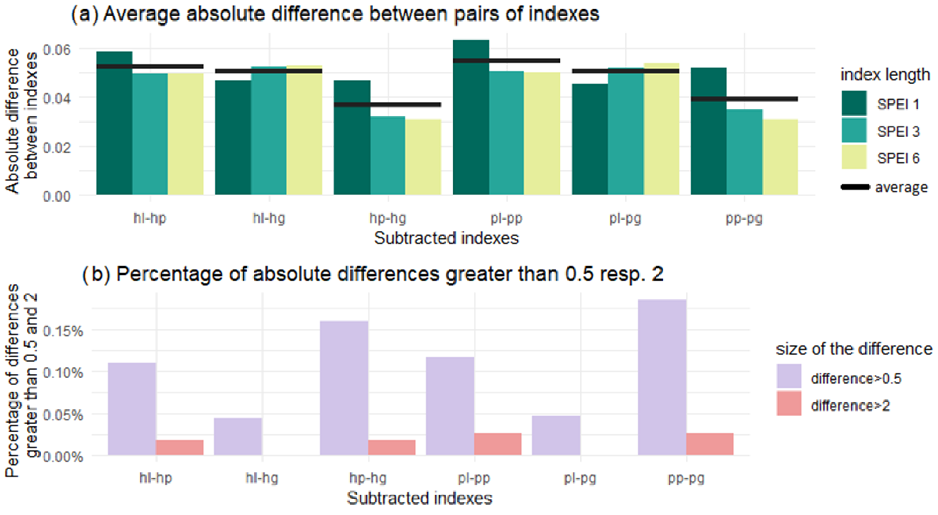
3.3. Comparison of Analysed Indices and Discussion

Although the absolute differences between indexes with different statistical distributions do not appear large, it is important to draw attention to the individual differences, which reach significant values under certain circumstances.

In

Table 6. The number of indices that were excluded due to the inability of the model to calculate the parameters of the distribution (1. criterion; “no-solution” cases), the number of indices that are not normally distributed (2. criterion; as an analogy to inappropriately fit of a statistical distribution of water balance), and the number of unlikely extremes (3. criterion; |SPEI| > 6). Indices excluded by a lower criterion were not included in the subsequent analysis with a higher criterion. The complete sample consists of 1,110,330 indices per distribution.

	Number of Eliminated Indices Due to Three Criteria
Elimination criterion →	1. Parameters fitting issues	2. Non-normal distribution	3. Unlikely extremes (|SPEI| > 6)	Total	Percentage of eliminated indices [%]
Distribution ↓
Log-logistic	0	15,834	0	15,834	1.43
Pearson III	3588	14,664	0	18,252	1.64
GEV	10,023	5070	0	15,093	1.36

, we present the assessment of excluded indices from applying our three criteria. Among the three investigated distributions, the most unfavourable outcomes arose when utilizing the Pearson III distribution, leading to the highest proportion of indices being excluded (1.64%).

The application of the Log-logistic distribution yielded satisfactory results, as we encountered no issues with fitting distribution parameters or encountering unlikely extremes. On the other hand, the Log-logistic distribution exhibited the highest occurrence of cases where indices did not adhere to a normal distribution (the cases when Log-logistic was an inappropriate distribution for fitting the water balance). Such instances accounted for 1.43% of the indices excluded in our analysis. Another disadvantage of this distribution is that the Log-logistic distribution underestimates extremes.

Applying the Generalized Extreme Value (GEV) distribution emerged as the most suitable approach based on our criteria, yielding the lowest number of excluded indices (1.36%). Despite its initial exclusion of a greater number of indices during the parameter fitting phase, the GEV distribution displayed fewer deviations from the normality condition in the subsequent step. Additionally, the exclusion of indices due to parameter fitting incompatibility is an automated process, effectively eliminating the majority of inaccurately estimated indices without necessitating further analyses, such as tests for normality.

The problem of no-solution cases was pointed out also in several other studies [7,23,24]. Our research agrees with the results of [23] in more no-solution cases with GEV compared to Log-logistic distribution. On the other hand, [24] experienced no fitting failure for both the GEV and Log-logistic distribution. Both mentioned results are related to the European region.

4. Conclusions

A few parameters (reference period, potential evapotranspiration equation, statistical distribution of water balance, etc.) can be modified when SPEI is calculated. The final value of SPEI could be significantly different when one of these modifiable parameters is changed.

In this article, we analysed how the choice of a statistical distribution of water balance can influence the final value of the SPEI.

(a)

Absolute difference testing:

First, the absolute difference between indices that differed only in statistical distribution (Log-logistic, GEV, or Pearson III distribution) was 0.05 on average, and about 99.9% of absolute differences were lower than 0.5 (0.5 is the threshold for another drought category).

Despite a relatively small absolute difference between indices with different statistical distributions, the next part of our study showed that changing the statistical distribution can influence the number of cases where it is not possible or appropriate to use this index, as well as extreme values of the index.

(b)

The number of no-solution cases and the number of inappropriate fits:

In some cases, the model of SPEI calculation is not able to estimate the parameters of the selected distribution, which leads to missing indices for the corresponding days (“no-solution” cases). If the parameters can be obtained, some indices should be eliminated due to inappropriate fit of a statistical distribution of water balance and, therefore, distorted results. According to our analysis based on the number of “no-solution” cases and the number of indices that do not meet the condition of normality of SPEI (what corresponds to an inappropriate fit of water balance), we can say that the smallest percentage of data losses can be obtained with GEV distribution (1.36%), followed by Log-logistic distribution (1.43%). The weakest results from the selected three distributions had Pearson III distribution (1.64% eliminated data) (see Table 6).

(c)

SPEI extremes:

From the perspective of index extremes, according to our results, the Log-logistic distribution underestimates extremes. On the other hand, in some cases, a higher number of unlikely high/low SPEI may occur (for example |SPEI| > 6). In this study (when the 39-year reference period was used), we found such extremes only with Pearson III distribution. When shorter reference periods were used, such extremes were observed in the other two analysed statistical distributions (Log-logistic and GEV). Some authors suggest implementing a threshold approach, where indices exceeding a predetermined threshold (e.g., ±3) are capped at that threshold value. In our study, such extreme values were not observed after excluding non-normally distributed indices. Consequently, we recommend performing a normality test on the indices and eliminating non-normally distributed indices rather than employing a fixed threshold approach.

(d)

Final comment

Nevertheless, since the Log-logistic distribution is recommended by many authors and is commonly used, our analysis reveals improved results when employing the Generalized Extreme Value (GEV) distribution. Approximately two-thirds of the excluded cases were omitted automatically via the calculation process as “no-solution cases”, which implies that without the implementation of additional analysis (such as testing for index normality), we would have fewer inaccurately estimated indices compared to using the Log-logistic or Pearson III distribution. At the same, in the case of Log-logistic distribution extremes may be underestimated.

When adhering to our proposed guidelines, such as the choice of the reference period, the procedure for handling and eliminating no-solution cases, and the normality test, it is possible to obtain a tool for calculating the SPEI index that does not exhibit issues with the distribution of extreme values and serves as a consistent tool for describing meteorological drought.

References

1. Faško, P.; Markovič, L.; Bochníček, O.; Pecho, J. Decadal Changes in Snow Cover Characteristics in Slovakia over the Period 1921–2020. In Proceedings of the EGU General Assembly 2020, Online, 4–8 May 2020. [Google Scholar]
2. Dančová, M.; Chovancová, Ľ.; Hinerová, A.; Malatinská, L.; Thumová, L.; Špalková, V.; Škultéty, J.; Gnida, M.; Pavlovič, V.; Szemešová, J.; et al. The Eight National Communication of the Slovak Republic on Climate Change: Under the United Nations Framework Convention on Climate Change and the Kyoto Protocol; Ministry of Environment of the Slovak Republic: Bratislava, Slovakia, 2023. [Google Scholar]
3. Trnka, M.; Balek, J.; Štěpánek, P.; Zahradníček, P.; Možný, M.; Eitzinger, J.; Žalud, Z.; Formayer, H.; Turňa, M.; Nejedlík, P.; et al. Drought Trends over Part of Central Europe between 1961 and 2014. Clim. Res. 2016, 70, 143–160. [Google Scholar] [CrossRef]
4. Nikolova, N.; Nejedlík, P.; Lapin, M. Temporal Variability and Spatial Distribution of Drought Events in the Lowlands of Slovakia. Geofizika 2016, 33, 119–135. [Google Scholar] [CrossRef]
5. Sönmez, K.F.; Komuscu, U.A.; Erkan, A.; Turgu, E. An Analysis of Spatial and Temporal Dimension of Drought Vulnerability in Turkey Using the Standardized Precipitation Index. Nat. Hazards 2005, 35, 243–264. [Google Scholar] [CrossRef]
6. Vicente-Serrano, S.M.; Beguería, S.; López-Moreno, J.I. A Multiscalar Drought Index Sensitive to Global Warming: The Standardized Precipitation Evapotranspiration Index. J. Clim. 2010, 23, 1696–1718. [Google Scholar] [CrossRef]
7. Beguería, S.; Vicente-Serrano, S.M.; Reig, F.; Latorre, B. Standardized Precipitation Evapotranspiration Index (SPEI) Revisited: Parameter Fitting, Evapotranspiration Models, Tools, Datasets and Drought Monitoring. Int. J. Climatol. 2014, 34, 3001–3023. [Google Scholar] [CrossRef]
8. Zhao, T.; Dai, A. CMIP6 Model-Projected Hydroclimatic and Drought Changes and Their Causes in the Twenty-First Century. J. Clim. 2022, 35, 897–921. [Google Scholar] [CrossRef]
9. Trnka, M.; Hlavinka, P.; Semenov, M.A. Adaptation Options for Wheat in Europe Will Be Limited by Increased Adverse Weather Events under Climate Change. J. R. Soc. Interface 2015, 12, 20150721. [Google Scholar] [CrossRef]
10. Balting, D.F.; AghaKouchak, A.; Lohmann, G.; Ionita, M. Northern Hemisphere Drought Risk in a Warming Climate. NPJ Clim. Atmos. Sci. 2021, 4, 61. [Google Scholar] [CrossRef]
11. Hlásny, T.; Csaba, M.; Seidl, R.; Kulla, L.; Merganičová, K.; Trombik, J.; Dobor, L.; Barcza, Z.; Konôpka, B. Climate Change Increases the Drought Risk in Central European Forests: What Are the Options for Adaptation? Lesn. Cas. 2014, 60, 5–18. [Google Scholar] [CrossRef]
12. Petrík, P.; Grote, R.; Gömöry, D.; Kurjak, D.; Petek-Petrik, A.; Lamarque, L.J.; Sliacka-Konôpková, A.; Mukarram, M.; Debta, H.; Fleischer, P., Jr. The Role of Provenance for the Projected Growth of Juvenile European Beech under Climate Change. Forest 2023, 14, 26. [Google Scholar] [CrossRef]
13. Potopová, V.; Trifan, T.; Trnka, M.; De Michele, C.; Semerádová, D.; Fischer, M.; Meitner, J.; Musiolková, M.; Muntean, N.; Clothier, B. Copulas Modelling of Maize Yield Losses–Drought Compound Events Using the Multiple Remote Sensing Indices over the Danube River Basin. Agric. Water Manag. 2023, 280, 108217. [Google Scholar] [CrossRef]
14. Török, P.; Dembicz, I.; Dajić-Stevanović, Z.; Kuzemko, A. Grasslands of Eastern Europe. In Encyclopedia of the World’s Biomes; Elsevier: Amsterdam, The Netherlands, 2020; pp. 703–713. ISBN 9780128160978. [Google Scholar]
15. McKee, T.B.; Nolan, D.J.; Kleist, J. The Relationship of Drought Frequency and Duration to Time Scales. In Proceedings of the Eighth Conference on Applied Climatology, Anaheim, CA, USA, 17–22 January 1993. [Google Scholar]
16. Labudová, L.; Labuda, M.; Takáč, J. Comparison of SPI and SPEI Applicability for Drought Impact Assessment on Crop Production in the Danubian Lowland and the East Slovakian Lowland. Theor. Appl. Climatol. 2017, 128, 491–506. [Google Scholar] [CrossRef]
17. Ionita, M.; Nagavciuc, V. Changes in Drought Features at the European Level over the Last 120 Years. Nat. Hazards Earth Syst. Sci. 2021, 21, 1685–1701. [Google Scholar] [CrossRef]
18. Moorhead, J.E.; Gowda, P.H.; Singh, V.P.; Porter, D.O.; Marek, T.H.; Howell, T.A.; Stewart, B.A. Identifying and Evaluating a Suitable Index for Agricultural Drought Monitoring in the Texas High Plains. J. Am. Water Resour. Assoc. 2015, 51, 807–820. [Google Scholar] [CrossRef]
19. Allen, R.G.; Pereira, L.S.; Raes, D.; Smith, M. Crop Evapotranspiration-Guidelines for Computing Crop Water Requirements; FAO Irrigation and drainage; FAO: Rome, Italy, 1998; p. 300. [Google Scholar]
20. Droogers, P.; Allen, R.G. Estimating Reference Evapotranspiration Under Inaccurate Data Conditions. Irrig. Drain. Syst. 2002, 16, 33–45. [Google Scholar] [CrossRef]
21. Sienz, F.; Bothe, O.; Fraedrich, K. Monitoring and Quantifying Future Climate Projections of Dryness and Wetness Extremes: SPI Bias. Hydrol. Earth Syst. Sci. 2012, 16, 2143–2157. [Google Scholar] [CrossRef]
22. Stagge, J.H.; Tallaksen, L.M.; Gudmundsson, L.; Van Loon, A.F.; Stahl, K. Candidate Distributions for Climatological Drought Indices (SPI and SPEI). Int. J. Climatol. 2015, 35, 4027–4040. [Google Scholar] [CrossRef]
23. Vicente-Serrano, S.M.; Beguería, S. Comment on ‘Candidate Distributions for Climatological Drought Indices (SPI and SPEI)’ by James H. Stagge et al. Int. J. Climatol. 2016, 36, 2120–2131. [Google Scholar] [CrossRef]
24. Stagge, J.H.; Tallaksen, L.M.; Gudmundsson, L.; Van Loon, A.F.; Stahl, K. Response to Comment on ‘Candidate Distributions for Climatological Drought Indices (SPI and SPEI)’. Int. J. Climatol. 2016, 36, 2132–2138. [Google Scholar] [CrossRef]
25. Bezdan, J.; Bezdan, A.; Blagojević, B.; Mesaroš, M.; Pejić, B.; Vranešević, M.; Pavić, D.; Nikolić-Đorić, E. SPEI-Based Approach to Agricultural Drought Monitoring in Vojvodina Region. Water 2019, 11, 1481. [Google Scholar] [CrossRef]
26. Blauhut, V.; Gudmundsson, L.; Stahl, K. Towards Pan-European Drought Risk Maps: Quantifying the Link between Drought Indices and Reported Drought Impacts. Environ. Res. Lett. 2015, 10, 014008. [Google Scholar] [CrossRef]
27. Potopová, V.; Štěpánek, P.; Možný, M.; Türkott, L.; Soukup, J. Performance of the Standardised Precipitation Evapotranspiration Index at Various Lags for Agricultural Drought Risk Assessment in the Czech Republic. Agric. For. Meteorol. 2015, 202, 26–38. [Google Scholar] [CrossRef]
28. Spinoni, J.; Naumann, G.; Vogt, J.; Barbosa, P. European Drought Climatologies and Trends Based on a Multi-Indicator Approach. Glob. Planet. Change 2015, 127, 50–57. [Google Scholar] [CrossRef]
29. Dukat, P.; Bednorz, E.; Ziemblińska, K.; Urbaniak, M. Trends in Drought Occurrence and Severity at Mid-Latitude European Stations (1951–2015) Estimated Using Standardized Precipitation (SPI) and Precipitation and Evapotranspiration (SPEI) Indices. Meteorol. Atmos. Phys. 2022, 134, 1–21. [Google Scholar] [CrossRef]
30. Oikonomou, P.D.; Karavitis, C.A.; Tsesmelis, D.E.; Kolokytha, E.; Maia, R. Drought Characteristics Assessment in Europe over the Past 50 Years. Water Resour. Manag. 2020, 34, 4757–4772. [Google Scholar] [CrossRef]
31. Melo, M.; Lapin, M.; Pecho, J. Climate in the Past and Present in the Slovak Landscapes—The Central European Context. In Landscapes and Landforms of Slovakia. World Geomorphological Landscapes; Springer: Berlin/Heidelberg, Germany, 2022; pp. 27–44. [Google Scholar]
32. Repel, A.; Zeleňáková, M.; Jothiprakash, V.; Hlavatá, H.; Blišťan, P.; Gargar, I.; Purcz, P. Long-Term Analysis of Precipitation in Slovakia. Water 2021, 13, 952. [Google Scholar] [CrossRef]
33. Gudmundsson, L.; Stagge, J.H. SCI: Standardized Climate Indices Such as SPI, SRI or SPEI. V.1.0-2. 2016. Available online: https://cran.r-project.org/web/packages/SCI/index.html (accessed on 1 August 2023).
34. Yimer, E.A.; Van Schaeybroeck, B.; Van de Vyver, H.; van Griensven, A. Evaluating Probability Distribution Functions for the Standardized Precipitation Evapotranspiration Index over Ethiopia. Atmosphere 2022, 13, 364. [Google Scholar] [CrossRef]
35. Nelder, J.A.; Mead, R. A Simplex Method for Function Minimization. Comput. J. 1965, 7, 308–313. [Google Scholar] [CrossRef]
Figure 1. Location of the study area in Europe (top) and stations included in the research (bottom). Stations lie between 112 m (station Veľký Meder) and 628 m (station Spišská Belá) above sea level.
Atmosphere 14 01464 g001
Figure 2. (a) The average absolute difference between pairs of indices that differs in statistical distribution (see Table 3); black lines represent the average absolute difference for all three studied index lengths; (b) percentage of absolute differences greater than 2 (pink) and 0.5 (violet).
Atmosphere 14 01464 g002
Figure 3. The number of no-solution cases for different modifications of SPEI calculation (type of SPEI; letters H and P after the name of distributions represent the used method for PET calculation: H = Hargreaves, P = Penman–Monteith) for all 13 used stations together (different stations are distinguished by colour). All shown indices are calculated based on a 39-year reference period.
Atmosphere 14 01464 g003
Figure 4. The number of cases when SPEI is not normally distributed for different modifications of SPEI calculation (Type of SPEI; letters H and P after the name of distributions represents the used method for PET calculation: H = Hargreaves, P = Penman–Monteith) for all 13 used stations together (different stations are distinguished by colour). All shown indices were calculated based on a 39-year reference period.
Atmosphere 14 01464 g004
Figure 5. Percentages of SPEI greater than 2 (blue) or lower than −2 (orange) for three studied statistical distributions.
Atmosphere 14 01464 g005