Article

Exploring the Centennial-Scale Climate History of Southern Brazil with Ocotea porosa (Nees & Mart.) Barroso Tree-Rings

by
Daniela Oliveira Silva Muraja
1,
Virginia Klausner
1,*,
Alan Prestes
1,
Tuomas Aakala
2,
Humberto Gimenes Macedo
1,3 and
Iuri Rojahn da Silva
1
1
Programa de Pós-Graduação em Física e Astronomia, Laboratóriode Registros Naturais, Instituto de Pesquisa e Desenvolvimento, Universidade do Vale do Paraíba, São José dos Campos 12244-390, SP, Brazil
2
School of Forest Sciences, University of Eastern Finland, 80130 Joensuu, Finland
3
Programa de Pós-Graduação em Pesquisa Operacional (PPG-PO), Universidade Federal de São Paulo (Unifesp)—Unidade Parque Tecnológico, São José dos Campos 12231-280, SP, Brazil
*
Author to whom correspondence should be addressed.
Atmosphere 2023, 14(9), 1463; https://doi.org/10.3390/atmos14091463
Submission received: 14 August 2023 / Revised: 13 September 2023 / Accepted: 15 September 2023 / Published: 20 September 2023
(This article belongs to the Special Issue Paleoclimate Reconstruction (2nd Edition))

Abstract

:
This article explores the dendrochronological potential of Ocotea porosa (Nees & Mart) Barroso (Imbuia) for reconstructing past climate conditions in the General Carneiro region, Southern Brazil, utilizing well-established dendroclimatic techniques. A total of 41 samples of Imbuia were subjected to dendroclimatic analysis to reconstruct precipitation and temperature patterns over the period from 1446 to 2011. Notably, we achieved the longest reconstructions of spring precipitation and temperature for the Brazilian southern region, spanning an impressive 566-year timeframe, by employing a mean chronology approach. To achieve our objectives, we conducted a Pearson’s correlation analysis between the mean chronology and the climatic time series, with a monthly temporal resolution employed for model calibration. Impressively, our findings reveal significant correlations with coefficients as high as |rx,P| = 0.32 for precipitation and |rx,T| = 0.45 for temperature during the spring season. Importantly, our climate reconstructions may elucidate a direct influence of the El Niño—South Oscillation phenomenon on precipitation and temperature patterns, which, in turn, are intricately linked to the natural growth patterns of the Imbuia trees. These results shed valuable light on the historical climate variability in the Southern Brazil region and provide insights into the climatic drivers affecting the growth dynamics of Ocotea porosa (Nees & Mart) Barroso.

1. Introduction

Numerous studies have shown that human actions have a significant impact on the Earth’s climate [1,2,3,4,5,6]. To comprehend the dynamics of this impact and unravel the intricacies of climate change, it becomes imperative to explore the characteristics of past climates. Paleoclimatology provides us with important insights into past climatic patterns, enabling a thorough analysis of how, when, and why climate changes have happened. This not only improves our comprehension of current climate oscillations but also enables us to forecast potential future changes and distinguish between naturally occurring variability and human-induced factors. Paleoclimatology becomes an essential tool for assessing the effects of human activity on nature and developing workable mitigation methods by illuminating the complex relationships between historical climates and current changes [1].
Understanding past climates relies on gathering climatic data from natural archives, including glacial deposits, river terraces, ice cores, varve sediments (annual layers of sedimentary rocks), corals, and tree growth rings [7]. Tree rings stand out among these records as a particularly useful tool for paleoclimatic research. The fact that trees are present in all types of landscapes and that their growth rings can be precisely dated to an annual level makes them a valuable and trustworthy source of historical climatic data.
When old or well-preserved long-dead trees are accessible, tree-ring series can provide a wealth of information covering enormous time scales. According to [8], these tree rings are useful markers of previous climates because of the influence of climatic variability on their attributes. The study of tree rings, or dendrochronology, is a useful method for determining environmental factors, climatic trends, and geophysical events. Insights into numerous environmental elements including light, temperature, water amount and availability, nutrition levels, and other stressors can be gleaned by evaluating tree rings under specified conditions, and these insights are useful when investigating climate dynamics [8]. The tree-ring series also makes it possible to look into how the climate has changed and fluctuated throughout the course of the trees’ lives.
The variation in temperature and precipitation patterns across different regions significantly influences tree growth, shaping the tree’s growth and dormancy cycles. As a result of the varying climatic conditions, areas that experience noticeable seasonal variations in temperature and precipitation have distinctive tree development patterns. Trees, on the other hand, must carefully decipher the nuanced environmental indications to determine the timing of their development and dormancy in places where seasons are less clearly defined. Tree-ring analysis is a crucial method for comprehending climatic fluctuations and their effects on various ecosystems because of the complex interactions between trees and seasonal climate patterns [8,9,10].
Studies on dendroclimatology have typically concentrated on areas with clearly defined seasonal climates, mostly in the temperate and boreal zones. Similar to this, in Brazil the southern region, which has distinct seasons, has been the focus of most dendroclimatological research. However, in some regions of the country, the climate lacks clearly defined seasons, and it is unclear whether or not there are seasonally visible tree rings [11].
Ocotea porosa (Nees & Mart) Barroso, also referred to as “Imbuia”, is one tree species that has distinguished itself as a valuable resource for dendrochronological studies in the southern region. Imbuia is a member of the Lauraceae family, and research by [12,13] shows that it has tremendous potential for dendrochronological studies. With individuals capable of living over 500 years old and exceptional examples like a tree unearthed in Santa Catarina claiming an astounding age of over 2700 years, Imbuia impressively stands out as one of the longest-living tree species in the Brazilian Araucaria woods.
The anatomy of Imbuia’s growth rings was thoroughly investigated by [14], leading to the establishment of a robust time series for southern Brazil. Their findings concluded that Imbuia can significantly contribute to dendrochronological studies in the region. Imbuia’s potential was further revealed when [15] used this species to research the “small summer” (also known as “veranico” locally) through the use of dendrochronology and morphometric analysis. Imbuia’s inclusion in dendrochronological research improves our knowledge of the climate dynamics and environmental processes unique to the southern region of Brazil and opens up new possibilities for investigation and understanding of past weather phenomena.
Despite its promising qualities, it is unclear how much the climate has affected the radial growth of Imbuia, which calls into question if it is a suitable candidate for dendroclimatic investigations. Given its potential for extraordinary lifespan (as highlighted by [14]), unraveling the species’ propensity to capture climatic signals in its growth rings gives a tremendous opportunity for climate reconstructions, especially in a location where paleoclimate data are sparse.
The main goals of this research are twofold: By measuring the tree ring width response to changes in temperature and precipitation in the South region of Brazil, it is first necessary to thoroughly evaluate and validate the dendroclimatic potential of Imbuia. This study aims to clarify the species’ climatic sensitivity and its capacity to operate as a trustworthy paleoclimate indicator. Second, the study tries to reconstruct the past climatic variability for the region using the knowledge collected from this evaluation.

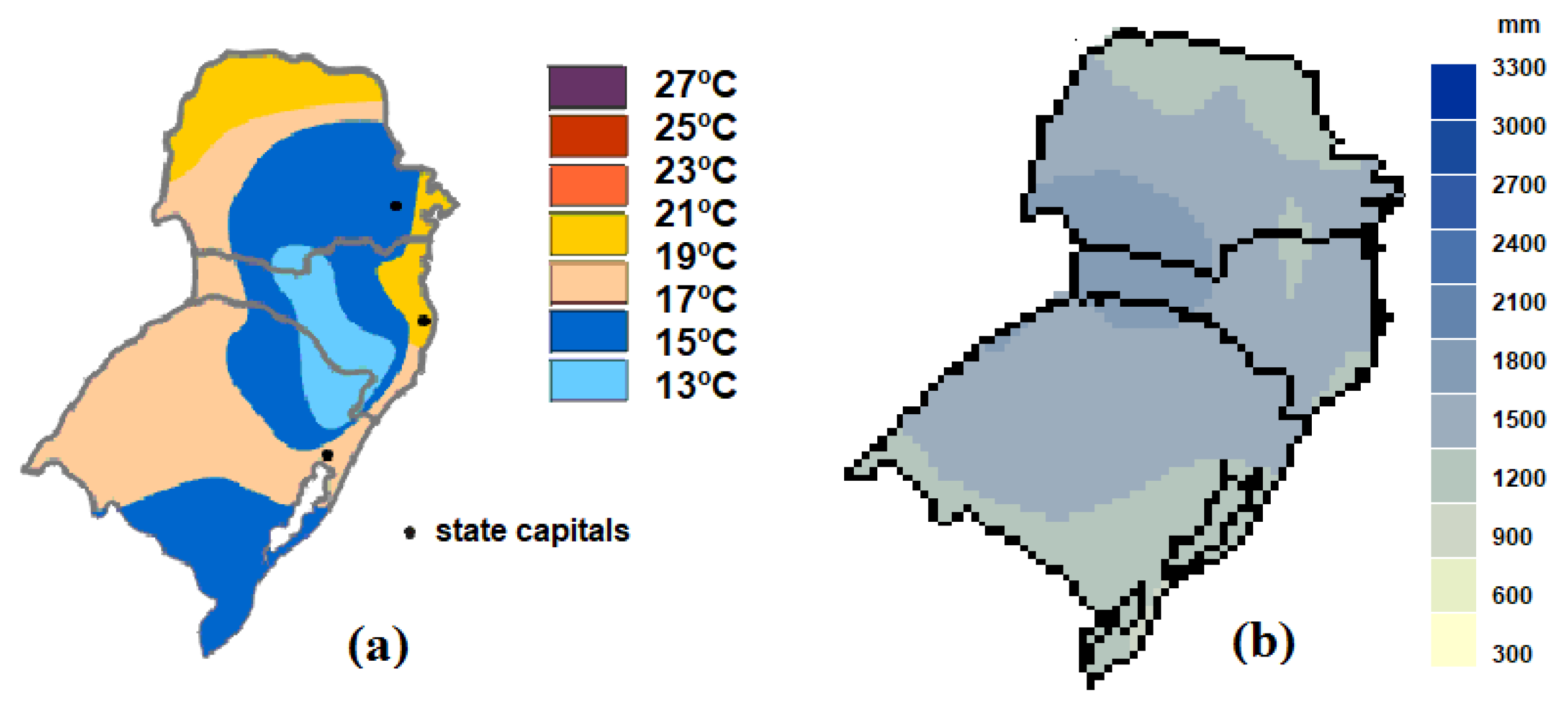
Climate of Southern Brazil

Given its vast territorial expanse, Brazil encompasses diverse climatic regimes, each influenced in distinct ways according to the region [16]. In this context, the southern part of Brazil is located below the Tropic of Capricorn and has a temperate climate, with a large section of its land at an altitude of 300 m above sea level (ASL).
Paraná (PR) state is located in the southern region of Brazil, along with the states of Rio Grande do Sul (RS) and Santa Catarina (SC). The climate in the South Region differs considerably from that of other regions in the country, and it is known for experiencing unique meteorological phenomena, seldom encountered in Brazil, such as snow and frosts [17].
The climatic characteristics of the South region are subtropical, with rainfall well distributed throughout the year. In a more specific classification, three types of climate are observed:
  • Cfb (cold winter with mild summer, wet winter, and summer),
  • Cfa (cold winter with hot summer, wet winter, and summer), and
  • Cwa (moderate temperatures with hot and rainy summer).
In these three climate types, there is a notable decrease in the precipitation index during winter, particularly in August, and a subsequent increase during the summer months. The standard thermal regime of the location is characterized as cold in winter and hot in summer. The average annual temperature for the region ranges between 14 °C and 22 °C, with altitudes above 1100 m experiencing an average temperature of 10 °C.
Southern Brazil is significantly influenced by mid-latitude systems, particularly frontal systems, which play a crucial role as rainfall mechanisms throughout the year [18]. In the context of medium latitudes, the annual temperature variation assumes great importance in defining the region’s climate. During winter, cold air masses from high latitudes penetrate the region, leading to lower temperatures [19]. These regular occurrences of polar masses, or cold air mass intakes, shape the distinct seasonal patterns experienced in the region [18].
While studies on polar masses are well-established, research on convective systems from frontal systems is relatively recent [18]. Additionally, other crucial weather systems operating in the region include Mesoscale Convective Complexes (MCC), predominantly active during spring and summer, and the South Atlantic Convergence Zone (SACZ), which influences the area from September to October and March to April. These systems are vital in explaining the renowned “Summer rains” experienced in Brazil [18].
The South Atlantic exerts an indirect yet significant influence on the climate of the region through the interaction of two distinct systems: the South Atlantic Anticyclone System (SAAS) generating the tropical marine mass, and the Polar Anticyclone producing the polar mass. The movement and interplay of these air masses, coupled with the warming of the Atlantic, are the primary drivers behind the copious rainfall experienced in Southern Brazil during spring and summer [20].
Moreover, throughout the year, the region is prone to abrupt climatic changes caused by polar fronts. These sudden shifts in weather contribute to significant deviations in annual rainfall, observed in both summer and winter, without exerting the same level of influence on thermal variability [21].
In the period from June to August, an average of 22 frontal system penetrations occur within the latitudinal range of 25° to 35° S [22]. The influx of cold fronts triggers the formation of instability lines and, when combined with other atmospheric phenomena, intensifies the development of convective precipitations. The dynamic interplay of these weather systems contributes to the region’s diverse and sometimes unpredictable climate patterns.
The South region, being located outside the tropics, receives comparatively less sunlight than tropical regions. However, during summer, the Earth’s position allows for increased insolation in this area, leading to higher evaporation rates. Additionally, its proximity to the Atlantic Ocean results in heightened cloudiness, consequently contributing to elevated levels of precipitation [23].
In the South region of Brazil, spring and summer are generally regarded as rainier seasons compared to autumn and winter. However, this pattern exhibits intriguing regional variations: (i) In the southern part of the South region, the rainiest season occurs during winter, whereas in the northern part, it is during the summer; and (ii) In the coastal regions, the distinction between dry and rainy seasons is less pronounced than in the continental regions. Coastal areas experience rainy winters and drier autumns, adding to the climatic diversity of the region [24,25].
Figure 1a showcases the average annual temperatures, while Figure 1b presents the annual precipitation averages for the Brazilian South region. The region’s pluviometric index averages around 1400 mm/year, while the average annual temperature hovers at approximately 18 °C, providing a comprehensive overview of the region’s climatic characteristics.

2. Materials and Methods

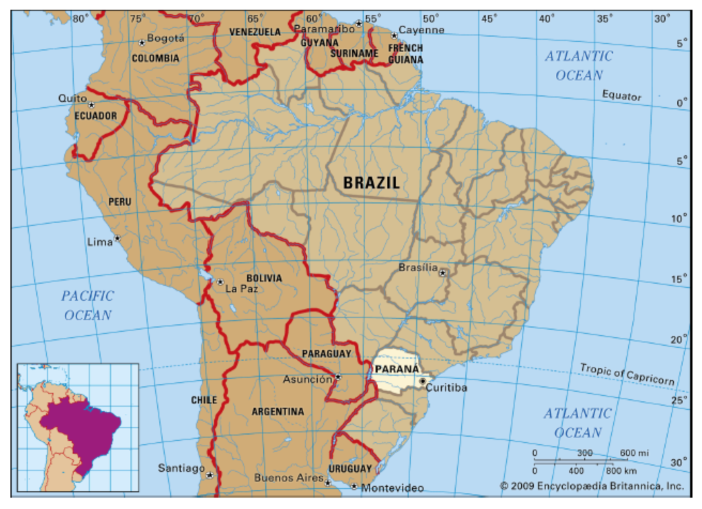
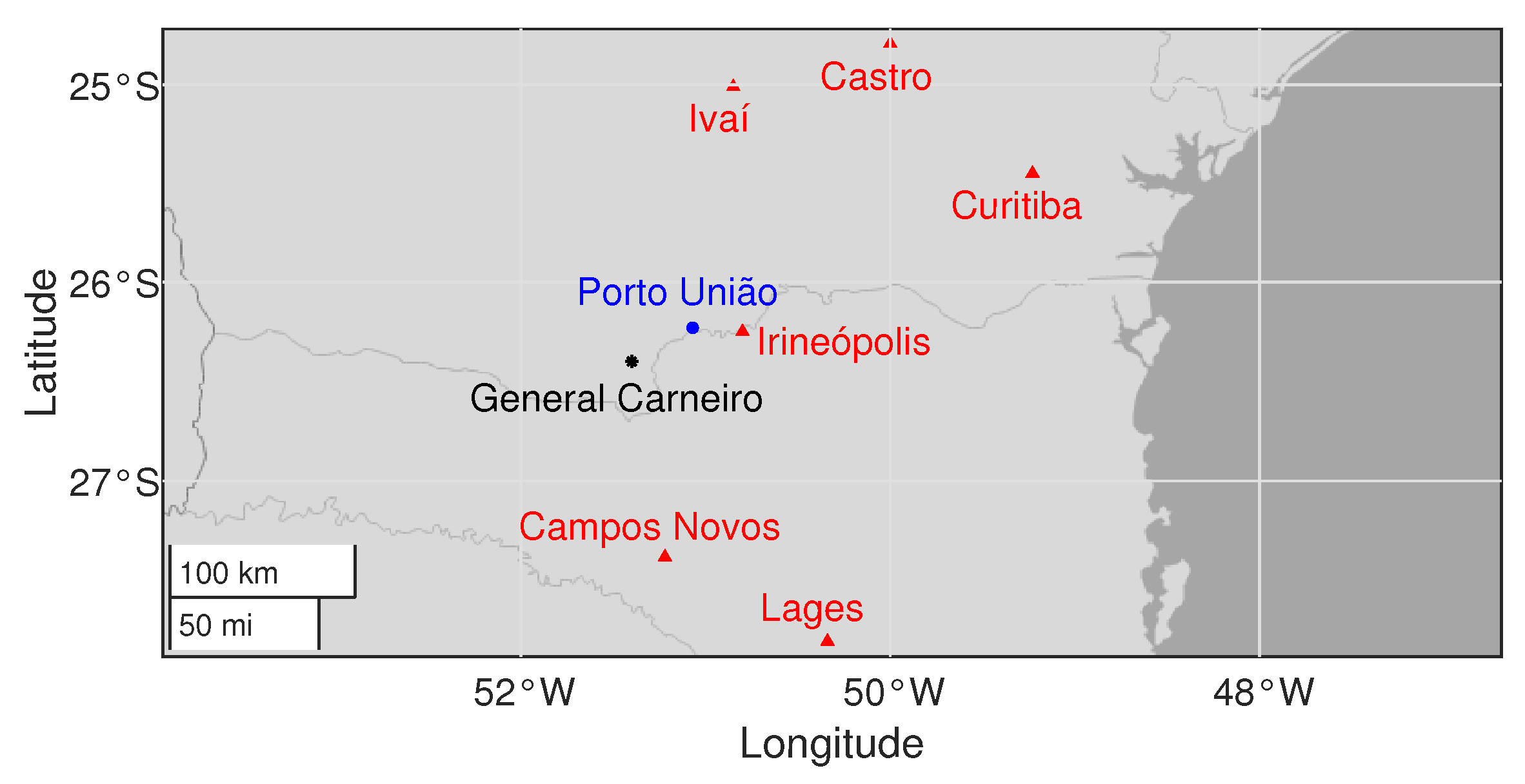
2.1. Research Location
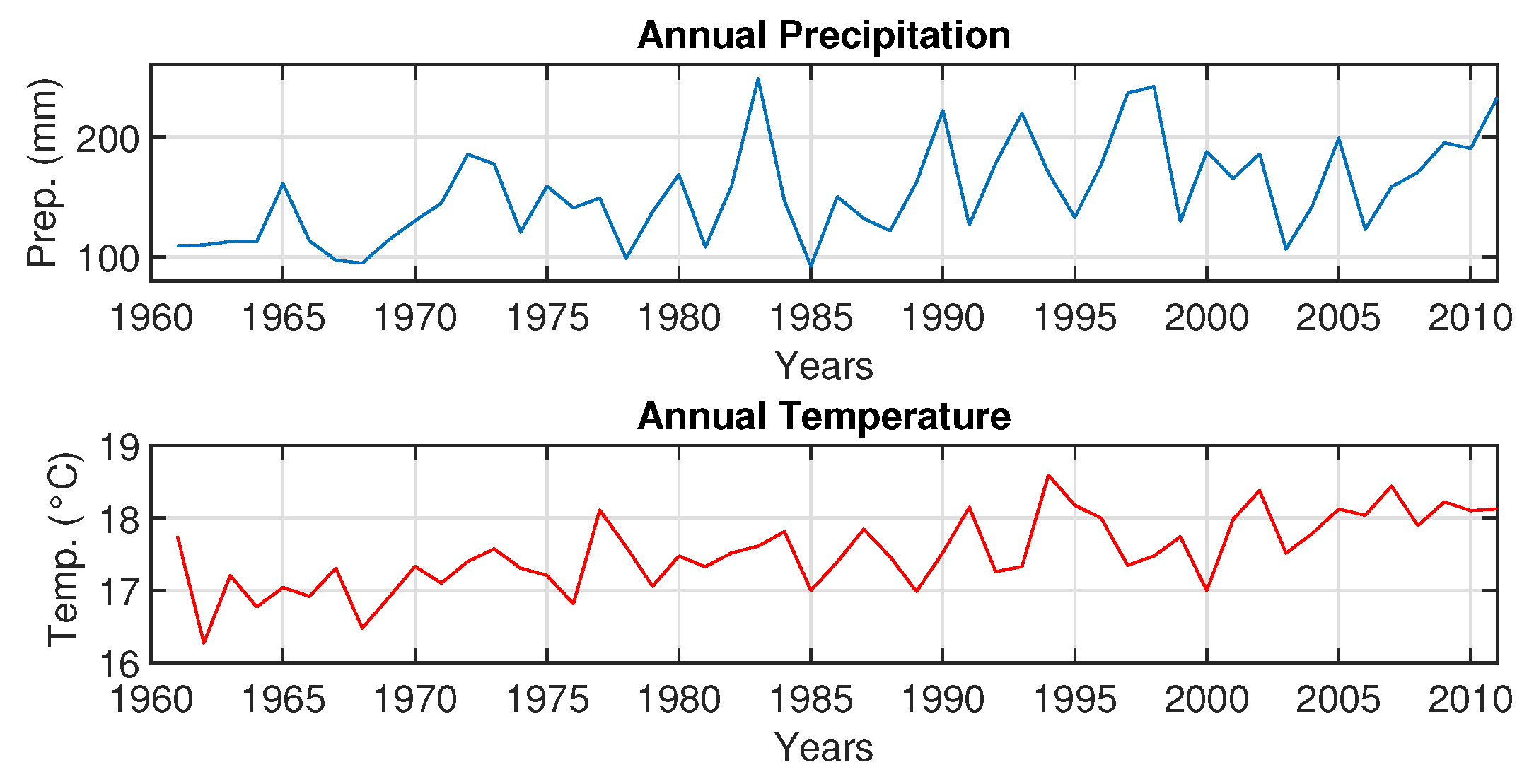
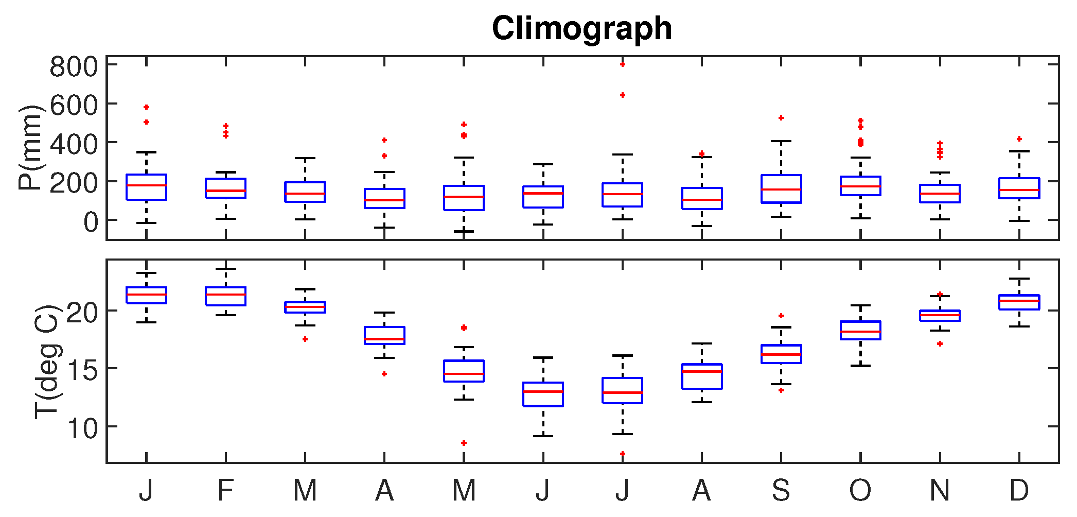
The municipality of General Carneiro (26°24′01.25″ S 51°24′03.91″ W) is situated within the state of Paraná (Figure 2), in the southern region of Brazil’s Southern Hemisphere. This city is positioned in the mesoregion of Southeast Paraná and the microregion of União da Vitória, at an altitude of 983 m [27]. The selection of this location is based on its clearly defined climatic conditions, which provide an ideal setting for conducting dendrochronological studies.

2.2. Climate Data

The city of Porto União, which is around 40 km from General Carneiro, provided the climate data used in this study (Figure 3). We used a robust multi-regression analysis filled with alternating least squares (ALS) to address gaps and missing data in the meteorological parameters of Porto União, i.e., precipitation and temperature. The same climatic characteristics were used in this method, which was based on data from meteorological stations in several nearby sites, including Lages, Castro, Curitiba, Campos Novos, Irineópolis, and Ivaí. Consequently, we were able to produce a more accurate and comprehensive climate dataset for our research because of this thorough data integration. The INMET website provides access to climatic data (https://bdmep.inmet.gov.br/#, accessed on 4 September 2023).
The climatic signals for temperature and precipitation are shown graphically in Figure 4, and they cover the years 1961 to 2011. Surprisingly, statistics from more recent decades show increased precipitation amplitudes. It’s worth noting that the pronounced increase in precipitation can be attributed to the particularly intense El Niño events of 1982–1983 and 1997–1998. Similarly, statistics for temperature reveal that the lowest yearly average occurred in 1962 and the highest average occurred in 1994.
Figure 5 presents a comprehensive monthly climograph illustrating both precipitation and temperature patterns spanning the entire year from 1961 to 2011. The precipitation trends exhibit a remarkable uniformity across the months. Based on the climograph analysis, it is clear that winter is the driest season, while spring and summer stand out as the wettest. Parallel to this, there is a consistent pattern to the temperature variations: spring and summer are marked by increased warmth, while winter is marked by a pronounced cold. In terms of temperature extremes, December, January, and February are the hottest, while June and July are the coldest month of the year. These observations collectively offer a concise portrayal of the climatic dynamics experienced throughout the year.

2.3. Sample Collection and Measurement

A total of 64 tree-ring samples were meticulously gathered through the non-destructive approach from 21 distinct Imbuia trees. The collection took place in the city of General Carneiro, situated within the southern Brazilian state of Paraná.
The non-destructive methodology employed entails delicately extracting wood samples using an increment borer, specifically at the diameter at breast height (DBH), at approximately 1.30 m above the ground. Executed in January 2013, this meticulous sampling endeavor encompassed the region as delineated in Figure 3.
The preparation of the tree-ring samples entailed a systematic sequence of steps to ensure accuracy and precision:
  • The samples underwent gentle drying under the shelter of shade-enclosed conditions.
  • Subsequently, they were meticulously polished on their transverse surfaces using 50–600 grit sandpaper to accentuate the tree-ring patterns.
  • Employing a stereomicroscope with 6 to 40× magnification and a fiber optic lighting system, the most exemplary sample radius was identified based on its tree-ring morphology.
  • Precise demarcations of the growth rings were executed.
  • The final stage encompassed the measurement of tree rings via a VELMEX measuring table, boasting a remarkable accuracy of 0.001 mm. This meticulous procedure ensured that no false or missing rings were overlooked.
The dating process commenced from the tree bark towards the pith. The most recent tree ring formed at the point of collection corresponds to the year 2011. Worth highlighting is the fact that the ring corresponding to the year 2012 had not yet completed its growth during the collection day due to Imbuia’s ring formation commencing in Spring/Summer.
Among the tree samples available, the oldest specimen partaking in this study boasts an impressive age of 566 years. Each tree’s measurements were subsequently transformed into diverse tree-ring chronologies.
To augment accuracy, the cross-validation technique employed a 50-year window. This methodology served to rectify counting errors, and it proficiently identified false rings and instances of partially missing rings [29]. It is noteworthy that of the initial 64 tree-ring samples, a discerning selection was made, ultimately comprising 41 samples that would contribute to the mean chronology, spanning the years from 1446 to 2011.

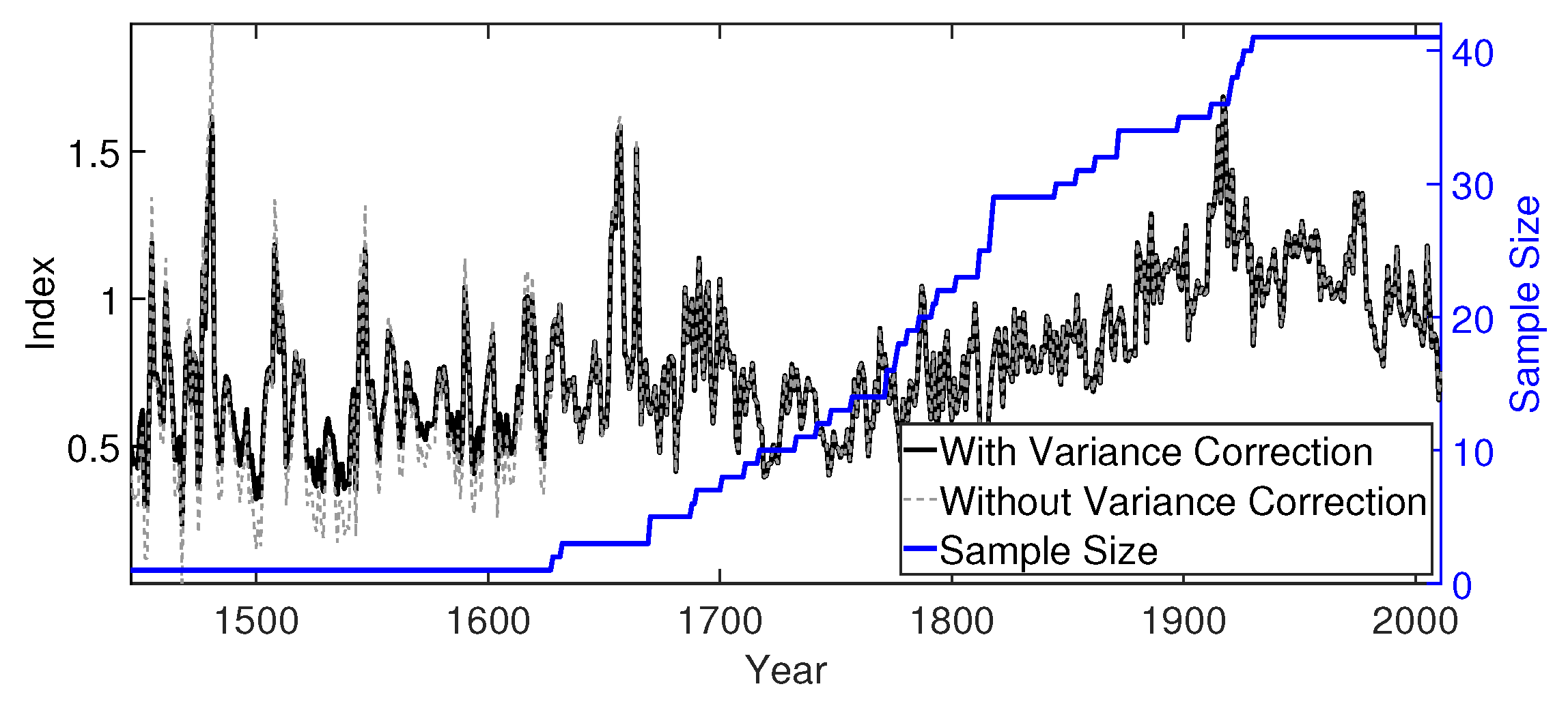
2.4. Estimation of the Mean Chronology

This article meticulously scrutinizes a total of 41 tree-ring samples, which were subjected to the Regional Curve Standardization (RCS) method [30,31]. The selection of this tree-ring standardization technique stems from our overarching objective of exploring the dendrochronological potential of Imbuia. The RCS method was chosen for its ability to conserve low-frequency signals, thereby ensuring the preservation of crucial climate variabilities [29].
The RCS process was executed through a series of steps: First, the time series of ring widths were realigned based on biological age to facilitate the computation of an average aging curve. Second, a 67% spline function was deployed to construct a seamless RCS curve, as detailed in [32]. This curve served as the foundation for calculating tree-ring indices as ratios. This strategic approach aimed to eliminate internal influences and amplify the climatic variabilities inherent in the tree-ring indices. Third, an essential re-alignment phase ensued, wherein all tree-ring series were re-calibrated according to the calendar year. This step paved the way for the construction of the mean chronology.
This study’s major result, the mean chronology, was carefully developed by using Tukey’s biweight robust mean approach [8,33]. In order to fully explore the dendroclimatic potential of Imbuia, we needed a trustworthy and representative mean chronology, which was produced as a result of this analytical approach.

2.5. Mean Chronology Variance Trend Correction

In the context of constructing a mean chronology using uneven yearly sample sizes, it’s important to recognize that as younger sample trees are integrated into the chronology, a natural diminishment backward in time can be expected. This phenomenon is due to the inclusion of more recent and younger samples in the chronology formation. This concept is expounded upon by [34], who noted that during certain time intervals where the number of samples decreases to values ranging between 5 and 10, a resultant increase in variance is observed when juxtaposed with intervals characterized by larger sample numbers.
To address the trend in variance arising from changing sample sizes, statistical techniques are employed. An approach introduced by [35] centers on rectifying variance trends by considering the maximum number of samples within a given interval. This correction involves the computation of the coefficient of variation ( C V s t d ) as
C V s t d = s s t d x ¯ s t d ,
where  s s t d  represents the standard deviation and  x ¯ s t d  signifies the mean of the interval with the maximum number of samples.
The correction for variance trends in time intervals lacking the maximum number of samples is calculated using the formula
I t cor = I t act I C V s t d C V k + I .
Here,  I t cor  denotes the corrected tree-ring index,  I t act  signifies the uncorrected index for the year t, I stands for the mean of the entire mean series (mean chronology), and  C V k  represents the coefficient of variation for time intervals not possessing the maximum number of samples.
Applying this method, the same variance trend correction technique was employed in our study. The corrected mean chronology (depicted as a black line), the change in sample size showcased as the number of samples (illustrated in blue), and the uncorrected series (rendered in light gray) are all visualized in Figure 6.
In this study, we have employed a straightforward methodology recommended by [33] to rectify bias in the variance of the tree-ring chronologies caused by fluctuations in sample size, also known as sample depth. This correction to the tree-ring chronology was only deemed necessary for periods where changes in sample size were equal to or below five samples.
To statistically assess the significance of our chronology signal spanning from 1962 to 2011, we utilized the Lilliefors Interval Exponential Distribution Test [36]. This evaluation was facilitated through the Seascorr software, which was implemented using MATLAB Release 2010, as detailed by [37].
An examination of both the histogram and the results of the Lilliefors test (depicted in Figure 7) leads to the observation that our chronology signal aligns well with a normal distribution. In particular, given that the critical value of  α  is below the threshold of 0.05, it substantiates the normal distribution of the mean chronology, a fact corroborated by the findings of [37].

2.6. Climate Series Analysis

We conducted Pearson’s Correlation analysis to establish the relationships between the General Carneiro chronology (Index) and the climatic time series for both temperature and precipitation. For confidence intervals about these correlations, we employed Monte Carlo simulation techniques, the specifics of which are detailed in [37].
To elucidate the climate-growth associations, the partial correlation of the mean chronology with precipitation, with the temperature influence removed, is mathematically defined as follows
r x , P . T = r x , P r x , T r P , T 1 r x , T 2 1 r P , T 2 .
In this equation,  r x , P r x , T , and  r P , T  denote the Pearson’s Correlation coefficients between the mean chronology and the precipitation time series, the mean chronology and the temperature time series, and the precipitation and temperature time series, respectively (as shown in Figure 8). This approach effectively isolates the influence of temperature on the relationship between the mean chronology and precipitation.
The correlation analysis is conducted iteratively, involving a total of 56 distinct seasons. Each of these 56 seasons represents a unique combination of the concluding month of tree-ring growth and the length of the season, as explained by [37]. To illustrate, if we consider that the tree-ring growth cycle concludes in March and we choose from season lengths 1, 3, 6, 12, we calculate correlations for each individual month, spanning from February of the preceding year through March of the current growth year. It’s important to note that this correlation corresponds to the year 1962, and the preceding year in our analysis is 1961 due to this seasonal consideration.
The goal of using partial correlation in this context, as stated by [37], is to take temperature into account when assessing the significance of precipitation’s impact on the mean chronology, and vice versa, to evaluate the significance of temperature while controlling for the influence of precipitation.

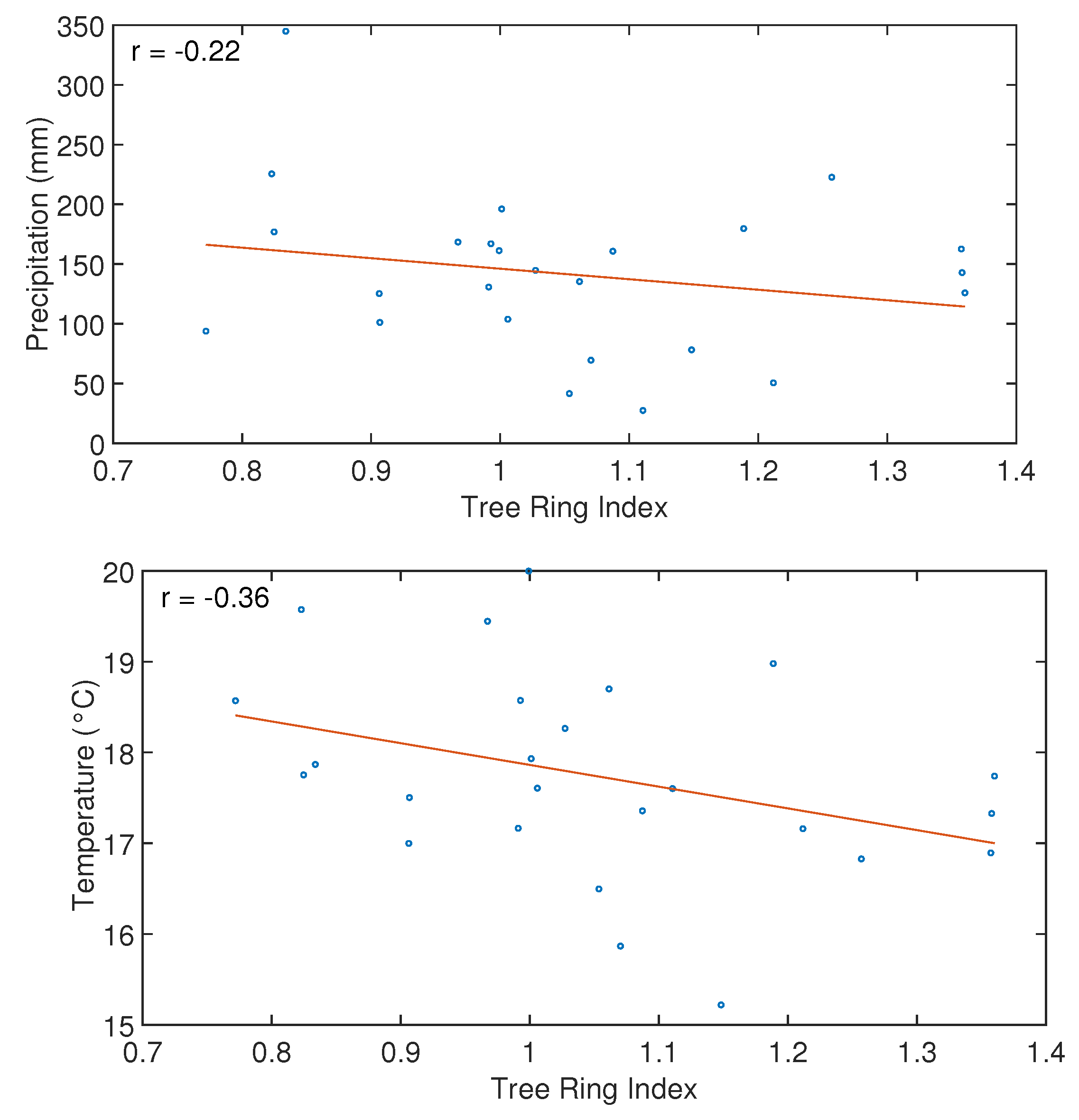
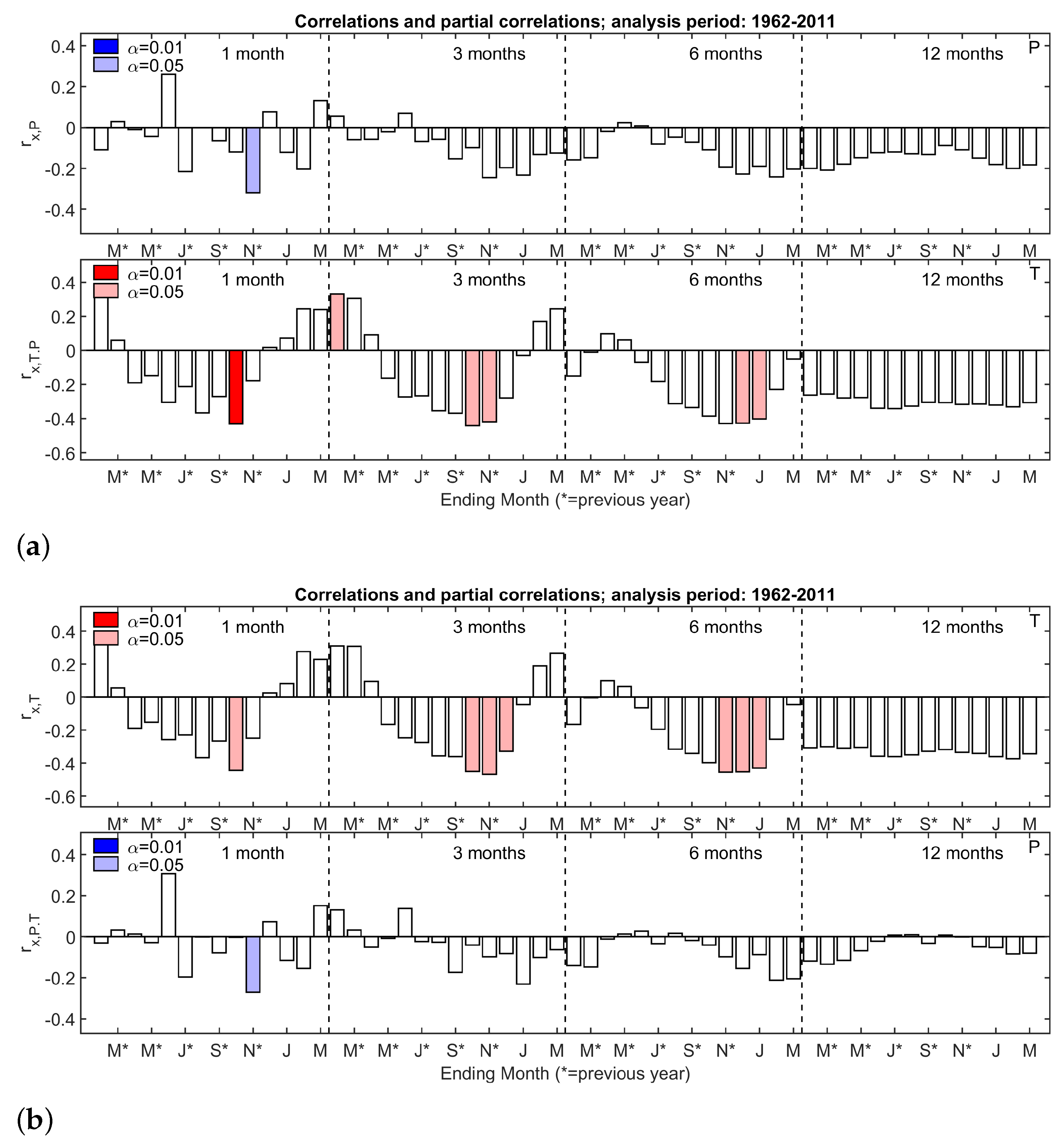
2.7. Climate-Growth Relationship and Climate Stability

By examining the dynamic interaction between the mean chronology and precipitation/temperature series, this paper considerably improves our understanding of how climate and growth interact. This study entails a thorough evaluation of the temporal stability of these relationships, which is accomplished using two different methodological approaches.
In the initial phase, the dataset was bifurcated into two discrete timeframes: the early-period (1962–1986) and the late-period (1987–2011), catering to the calibration and verification procedures. Calibration was executed within the early-period, followed by verification within the late-period. This involved computing Pearson correlation coefficients (r) for each interval, encompassing the entire period. Complementary metrics, namely reduction error (RE) and coefficient of efficiency (CE) [8], were also computed to gauge the effectiveness of the calibration model in approximating the actual values of the original climate series. This multi-pronged approach is pivotal to ensuring the fidelity of the calibration model’s predictions.
Subsequently, in the second phase, the stability of the association between the mean chronology and the primary climate variables was further assessed using Pearson correlation [33]. The central tenet of this stability analysis is to identify temporal segments where the correlation between the proxy data and climate variables remains consistent. To realize this, the Pearson correlation for each independent predictor variable was scrutinized, probing the temporal stability in the linkage between tree growth and climate signals across the entire period, as well as within its individual sub-periods.

3. Results and Discussion

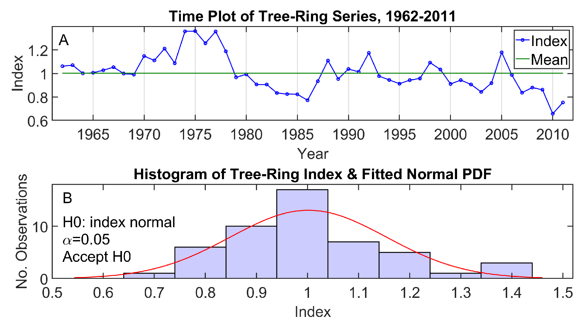
3.1. Climate Series Analysis

In Figure 8a, the correlation between the mean chronology and precipitation (top panel) is negatively significant, particularly in November ( | r x , P | = 0.32  and  α = 0.05 ). This negative correlation is most pronounced during the spring months. Notably, the temperature partial correlation (bottom panel) demonstrates a relatively strong negative correlation, particularly noticeable in October. The significance of this partial correlation also is intensified during the spring months, centering in October and November, as observed in a three-month moving average.
Turning to Figure 8b, it displays the simple correlation of temperature with the mean chronology (top panel). In October, a significant correlation is seen ( | r x , T | = 0.45  and  α = 0.05 ). Additionally, throughout the spring season, particularly in November, the precipitation partial correlation (bottom panel) becomes noticeably significant. This negative precipitation partial correlation coincides with a very rainy spring season, which is consistent with the wetness stress brought on by higher spring precipitation levels.
Excessive spring/summer rainfall can be considered an external climatic factor that adversely affects the growth of Imbuia trees in the study area. The surplus water availability resulting from elevated spring rainfall implies a growth disadvantage for these trees. This increased water supply may be associated with the El Niño—Southern Oscillation (ENSO) events, contributing to amplified precipitation and prolonged rainy periods in southern Brazil during spring and summer. Moreover, our findings highlight that tree growth in General Carneiro exhibits a negative response to higher temperatures in spring months.

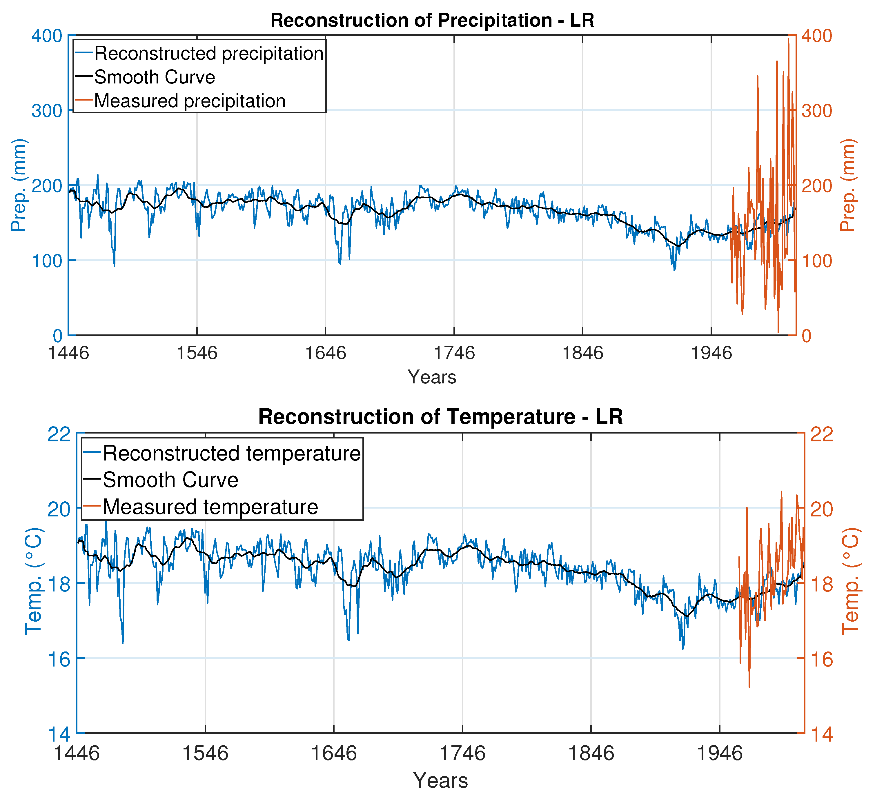
3.2. Climatic Reconstructions

We will provide an extensive overview of the reconstruction of climate variables, with a particular emphasis on precipitation for October and temperature for November, both of which occur during spring. Our objective is to describe variations that date back to 1446. The initial phase involved determining the dispersion of the input data in Linear Regression (LR), involving mean chronology and spring precipitation/temperature time series related to the early-period of 1962–1986. This dispersion analysis is illustrated in Figure 9.
Based on these findings, we derived Equations (2) and (3), which serve as the foundation for reconstructing variations in precipitation and temperature since 1446. In these equations, X represents the mean chronology. The reconstruction formulas using linear regression are as follows
P r e p = 88.04 X + 234.12 ;
T e m p = 2.39 X + 20.26 .
The second step involved assessing the temporal stability of the relationship between the mean chronology and our primary climate variables, which is termed calibration. This assessment was conducted using Pearson correlation. We divided the analysis period, 1962–2011, into two sub-periods: 1962–1986 (early-period) and 1987–2011 (late-period). This division allowed us to examine potential changes in the correlation dynamics.
In Table 1, the RE (0.031) and CE (0.021) values, as applied to the precipitation dataset, align admirably with the established acceptance criteria ( > ; 0 ) for endorsing the reconstruction model. However, a different scenario emerges for temperature, where CE (−0.876) assumes a negative value. It’s worth noting that interpreting these values, as pointed out by [38], warrants some circumspection, particularly when the data exhibits pronounced correlations or trends.
According to [38], the contextual backdrop should include the presence of high correlation or trends in the data while considering the RE and CE values. In this light, the RE and CE metrics function as estimators of the efficacy of the linear relationship existing between the climate series and the reconstructed series. When RE values assume a positive orientation and tend toward 1, it signifies the model’s capacity for adept climate reconstruction [34,39].
When considering precipitation as the primary variable, the split-time correlation analysis reveals temporal consistency in the relationship between tree ring width and November precipitation. The correlations stand at 0.22 for the early-period and 0.43 for the late-period, as delineated in Table 1. The divergence in these values within the late-period prompts a prudent approach in both climatic reconstructions and the interpretation of the relationship between natural tree growth and precipitation. This divergence implies that the relationship between tree growth and precipitation may have experienced notable changes during the late 20th century, warranting further scrutiny.
Conversely, when focusing on temperature as the primary climate variable, the obtained correlation values are 0.36 for the early-period and 0.35 for the late-period. This uniformity in correlations across the two sub-periods, despite their temporal separation, suggests a lack of evidence for significant temporal instabilities. These correlation values remain practically constant throughout the entire 1962–2011 analysis timeframe.
Research by [40] conducted in Florida demonstrated that temperature did not particularly affect the growth of long-leaf pine (P. palustris). Conversely, in Missouri, [41] discovered an inverse relationship between average temperatures and the width of oak tree rings. However, in both cases, there was a correlation between precipitation and annual ring width. This highlights the importance of a singular climatic factor, even though related factors may influence growth dynamics.
In this study, with a focus on the seasons in the southern hemisphere, it was observed that temperature during the summer months also had a pronounced influence on the growth of General Carneiro’s Imbuia trees (see Figure 8a—bottom panel-partial correlation-3-month seasons). This factor may show a significant positive impact during the three months of summer (December, January, and February) with increased exchange activity, while the other months exhibited a less active exchange rate. This pattern is in line with prior research by [42,43], which established the plant growth period as spring and summer, contrasting with the dormant period during autumn and winter.
In the context of southern Brazil, [44] conducted a study indicating a pronounced decline in growth during the autumn and winter months, coupled with peak growth in the summer months for Lauraceae family species. Furthermore, [13], utilizing the same species, demonstrated that both precipitation and temperature significantly impact annual growth. [45] revealed that their Araucaria angustifolia samples respond to both temperature and precipitation, a phenomenon also mirrored in Cedrela fissilis samples as documented by [46]. However, [47]’s study suggests that trees can potentially respond to either a singular climatic factor or a combination of factors during months of heightened plant exchange activity. Collectively, these findings underscore the intricate nature of the relationship between tree growth and climatic factors, where the dominant influencer could be attributed to one or multiple climatic variables.
We continued with the reconstruction of both climatic parameters despite the potential difficulties presented by the link between temperature and tree ring widths, as suggested by the CE and RE statistics. The resultant reconstructions, depicted in Figure 10, were derived from the month of November (October) data for precipitation (temperature), coinciding with the spring season in the southern hemisphere.
Through these reconstructions, we can identify periods characterized by elevated and diminished levels of precipitation and temperature. Peaks in these variables are noticeable around the years 1450, 1500, 1530, 1600, 1640, 1680, 1720, and 1750, while valleys are apparent circa 1480, 1510, 1555, 1625, 1660, 1695, 1735, and 1920. Notably, beginning from the year 1920, a consistent escalation in average precipitation and temperature levels is discernible, with a more pronounced upsurge observed after the 1950s. The escalation in temperature could be attributed to anthropogenic-driven climate change.
In these specific years, the outcomes suggest the potential occurrence of significant climatic or geophysical events, such as El Niño (associated with heightened rainfall) and La Niña (linked to diminished precipitation) events. Precipitation in Pelotas City (Southern Brazil) correlates with ENSO events as established by [48]. Our findings align with the study conducted by [45] in southern Brazil, demonstrating a close relationship between Araucaria angustifolia tree-ring growth and variations in temperature and precipitation. This connection may extend to nonlinear impacts of solar variability and the El Niño-Southern Oscillation, though these aspects warrant further investigation in our forthcoming research.
Using a tree-ring series from Nectandra oppositifolia Nees and Mart, a tree that, like Imbuia, is a member of the Lauraceae family, provides an interesting comparison. The study of [49], which covered the years 1843 to 2013, emphasized how susceptible trees are to excessive rain, which is frequently linked to El Niño events, particularly in the Brazilian state of Santa Catarina. Additionally, the more recent research by [50] highlighted the long-lasting and strong impact of El Niño on interhemispheric changes and tree development over a considerable 258-year period. This improves our comprehension of the dynamics of hydroclimatic variability and has implications for forecasting.
According to [51], the effects of intense ENSO events go beyond trees and can have a considerable impact on agricultural productivity. According to [52], dendrochronology is a useful tool for understanding the complex ocean-atmosphere dynamics that underlie occurrences like El Niño. Tree-ring reconstructions can provide information on past occurrences of ENSO events through the analysis of teleconnection responses, even if they may not directly reveal the particular mechanisms causing warm or cold ENSO events, such as Kelvin waves.
As a result, additional research is necessary to identify potential El Niño signals in tree-ring series and to understand their fluctuations and responses in the context of changing climatic conditions.
In the broader context of global climatic patterns, a 531-year precipitation reconstruction for Huashan corroborated a significant association between the precipitation in northern China and ENSO [53]. Remarkably dry years recorded in the reconstruction of [53] aligned with documented historical El Niño events. Chronologies from moisture-sensitive coniferous areas in New Mexico and southern Colorado showed a similar resonance with ENSO indices, including SOI, and provided a 1000-year reconstruction of precipitation. It is noteworthy that some of the rainy years in this reconstruction, including 1484, 1720, 1816, and 1941, occurred at the same time as ENSO-related events [54].
However, it is important to acknowledge certain limitations in our results. The correlations between climatic variables and the ring width index are moderate at best; the monthly climate data in the calibration phase only explains around 22% to 36% of the variation in the ring width index. Moreover, the climate reconstruction from 1446 to 1626 relies on a single old tree, a factor that should be considered when interpreting our findings.

4. Summary

In conclusion, our study addressed crucial aspects of climate-growth relationships in the General Carneiro region of Southern Brazil, employing the powerful technique of dendrochronology. This approach has allowed us to reconstruct precipitation and temperature patterns over an impressive 566-year period, providing valuable insights into the historical climate variability of this region.
Our findings indicate the complex relationship between temperature and precipitation, demonstrating their vast impact on the growth of Imbuia trees in Southern Brazil. During the spring season, we found consistent correlations with coefficients as high as 0.32 for precipitation and 0.45 for temperature. These results imply that temperature in this location influences the growth dynamics of Ocotea porosa (Nees & Mart) Barroso.
The climatic reconstructions we have derived accentuate discernible high and low-temperature peaks, closely mirroring the corresponding precipitation patterns. This notable consistency between temperature and precipitation underscores their intertwined impact on Imbuia growth in Southern Brazil. The years 1450, 1500, 1530, 1600, 1640, 1680, 1720, and 1750 appear to be punctuated by climatic events, potentially including occurrences of El Niño events characterized by heightened rainfall. A significant transition emerged from 1950 onward, portraying a sustained escalation in both average rainfall and temperature. Notably, a remarkable peak in the year 1950 strongly hints at the emergence of global warming trends. This latter observation is indicative of a broader trend associated with global warming.
The longevity of our tree-ring series, spanning 566 years in the mean chronology, is a significant contribution, offering unprecedented access to the climatic history of this region. However, it’s essential to acknowledge certain limitations. The moderate correlations between climatic variables and the ring width index (explaining only around 32% to 45% of the variation) indicate the existence of additional factors influencing tree growth in this region.
For local implications, our study emphasizes the sensitivity of Imbuia trees to climatic factors, especially during the spring season. This information can be useful for managing local forests and promoting conservation, assisting stakeholders in selecting tree species and predicting their growth in response to climate change.
The discrepancies seen in our study, such as the divergence in temperature-growth connections in the late 20th century, also point to changing climatic dynamics in the area. This emphasizes how crucial it is to do ongoing research to track and comprehend these changes, particularly in the context of climate change.
In summary, our research highlights the importance of native tree species in climate studies while also offering historical perspectives on the climate of Southern Brazil. It urges further research into the complex relationships that exist between trees and their surroundings. This knowledge is essential for both local conservation efforts and broader climate science pursuits.

Author Contributions

V.K., A.P. and T.A. provided valuable guidance and supervision to D.O.S.M. throughout the investigation of the paleoclimate reconstruction. Also, V.K. and A.P. made substantial contributions to this work, encompassing data collection, organization, analysis, and interpretation, including the creation of the analysis graphs. D.O.S.M. enriched the introduction and discussion section and played a part in obtain the INMET dataset. H.G.M. was the driving force behind the algorithm development for mean chronology variance trend correction. I.R.d.S. played a pivotal role in developing the mean chronology, a significant component of his thesis. All authors have read and agreed to the published version of the manuscript.

Funding

This research received no external funding.

Institutional Review Board Statement

Not applicable.

Informed Consent Statement

Not applicable.

Data Availability Statement

To obtain the data for this study, please contact the authors via email.

Acknowledgments

The authors would like to thank FAPESP (Fundação de Amparo à Pesquisa do Estado de São Paulo.) for its assistance in the Prestes A. FAPESP project—(2009/02907-8), and CNPq (Conselho Nacional de Desenvolvimento Científico e Tecnológico) for its assistance in the Klausner V. CNPq projects—305249/2018-5 and 308258/2021-5.

Conflicts of Interest

The authors declare no conflict of interest.

References

  1. Keith, D.A.; Raymond, S.B.; Thomas, F.P. Paleoclimate, Global Change and the Future, 1st ed.; Springer: Berlin/Heidelberg, 2003. [Google Scholar]
  2. Cook, E.R.; Woodhouse, C.A.; Eakin, C.M.; Meko, D.M.; Stahle, D.W. Long-Term Aridity Changes in the Western United States. Science 2004, 306, 1015–1018. [Google Scholar] [CrossRef] [PubMed]
  3. Mann, M.E.; Zhang, Z.; Hughes, M.K.; Bradley, R.S.; Miller, S.K.; Rutherford, S.; Ni, F. Proxy-based reconstructions of hemispheric and global surface temperature variations over the past two millennia. Proc. Natl. Acad. Sci. USA 2008, 105, 13252–13257. [Google Scholar] [CrossRef] [PubMed]
  4. Sheppard, P.R. Dendroclimatology: Extracting climate from trees. WIREs Clim. Chang. 2010, 1, 343–352. [Google Scholar] [CrossRef]
  5. Fichtler, E. Dendroclimatology using tropical broad-leaved tree species—A review. Erdkunde 2017, 71, 5–22. [Google Scholar] [CrossRef]
  6. Foroozan, Z.; Grießinger, J.; Pourtahmasi, K.; Bräuning, A. 501 Years of Spring Precipitation History for the Semi-Arid Northern Iran Derived from Tree-Ring δ18O Data. Atmosphere 2020, 11, 889. [Google Scholar] [CrossRef]
  7. Fritts, H.C. Reconstructing Large-Scale Climatic Patterns from Tree-Ring Data; The University of Arizona Press: Tucson, AZ, USA, 1991. [Google Scholar]
  8. Fritts, H.C. Tree Rings and Climate; The University of Arizona Press: Tucson, AZ, USA, 1976. [Google Scholar]
  9. Schweingruber, F.H. Tree Rings—Basics and Applications of Dendrochronology; Kluwer Academic Publishers: Alphen aan den Rijn, The Netherlands, 1983. [Google Scholar]
  10. Mann, M.E.; Bradley, R.S.; Hughes, M.K. Northern hemisphere temperatures during the past millennium: Inferences, uncertainties, and implications for understanding recent climate change. Geophys. Res. Lett. 1999, 26, 759–762. [Google Scholar] [CrossRef]
  11. Boninsegna, J.; Argollo, J.; Aravena, J.; Barichivich, J.; Christie, D.; Ferrero, M.; Lara, A.; Le Quesne, C.; Luckman, B.; Masiokas, M.; et al. Dendroclimatological reconstructions in South America: A review. Palaeogeogr. Palaeoclimatol. Palaeoecol. 2009, 281, 210–228. [Google Scholar] [CrossRef]
  12. Mattos, P.P.; Oliveira, M.F.; Agustini, A.F.; Braz, E.M.; Rivera, H.; Oliveira, Y.M.M.; Rosot, M.A.D.; Garrastazu, M.C. Aceleração do crescimento em diâmetro de espécies da Floresta Ombrófila Mista nos últimos 90 anos. Pesqui. Florest. Bras. 2010, 30, 319–326. [Google Scholar] [CrossRef]
  13. Reis-Avila, G.; Oliveira, J.M. Lauraceae: A promising family for the advance of neotropical dendrochronology. Dendrochronologia 2017, 44, 103–116. [Google Scholar] [CrossRef]
  14. Cosmo, N.L.; Lira, P.K.; Moresco, G.C.; Soffiatti, P.; Sousa, T.R.; Vasconcellos, T.J.; Lisi, C.S.; Botosso, P.C. Dendroecologia da espécie Ocotea porosa (Imbuia), Lauraceae, em áreas de Floresta Ombrófila Mista na região de Faxinal do Céu, Paraná. In Proceedings of the 5th South American Dendrochronological Fieldweek, Faxinal do Céu, Paraná, Brazil, 5 January 2009. [Google Scholar]
  15. Santos, A.T.D.; Mattos, P.P.D.; Braz, E.M.; Rosot, N.C. Determinação da época de desbaste pela análise dendrocronológica e morfométrica de Ocotea porosa (Nees & Mart.) Barroso em povoamento não manejado. Ciência Florest. 2015, 25, 699–709. [Google Scholar]
  16. Vanhoni, F.; Mendonca, F. O Clima do litoral do Estado do Paraná. Rev. Bras. Climatol. 2008, 3, 25423. [Google Scholar] [CrossRef]
  17. Hiera, M.D.S.; Edvard, E.A.V. As chuvas de junho e a primeira onda de frio intenso de 2013: A atuação dos sistemas atmosféricos e o ritmo climático para a região de Maringá. Rev. Programa Pós-graduação Geogr. 2014, 6, 78–94. [Google Scholar]
  18. Nery, J.T. Dinâmica Climática da Regiã Sul do Brasil. Rev. Bras. Climatol. 2005, 1, 1. [Google Scholar]
  19. Quadro, M. Estudo de episódios de zonas de convergência do Atlântico Sul (ZCAS) sobre a América do Sul. Rev. Bras. Geof. 1999, 17. [Google Scholar] [CrossRef]
  20. Nimer, E. Climatologia do Brasil; IBGE: Rio de Janeiro, Brazil, 1989. [Google Scholar]
  21. Leal, P.C. Sistema Praial Moçambique—Barra da Lagoa—Ilha de Santa Catarina—Brasil: Aspectos Morfológicos, Morfodinâmicos, Sedimentológicos e Ambientais. Master’s Thesis, Universidade Federal de Santa Catarina, Santa Catarina, Brazil, 1999. [Google Scholar]
  22. Oliveira, A.S. Interações Entre Sistemas na América do Sul e Convecção na Amazônia. Master’s Thesis, Instituto Nacional de Pesquisas Espaciais, São José dos Campos, Brazil, 1986. [Google Scholar]
  23. Dittberner, M.R. Causas e Efeitos das Turbulências nas Operações Aéreas do Aeroporto Internacional Hercílio Luz. Bachelor’s Thesis, Departamento de Geografia—UFSC, Santa Catarina, Brazil, 2000. [Google Scholar]
  24. Rao, V.B.; Hada, K. Characteristics of Rainfall over Brazil: Annual Variations and Connections with the Southern Oscillations. Theor. Appl. Climatol. 1990, 42, 81–91. [Google Scholar] [CrossRef]
  25. Studzinski, C.D. Um estudo da precipitação na Região Sul do Brasil e sua Relação com os Oceanos Pacífico e Atlântico Tropical Sul. Master’s Thesis, Instituto Nacional de Pesquisas Espaciais, São José dos Campos, Brazil, 1995. [Google Scholar]
  26. INMET. Normais Climatológicas 1931–1990. 1995. Available online: http://www.inmet.gov.br (accessed on 9 February 2020).
  27. Gerais, D. Prefeitura de General Carneiro. 2020. Available online: http://www.generalcarneiro.pr.gov.br/municipio/dados-gerais/ (accessed on 20 October 2020).
  28. Britannica, The Editors of Encyclopaedia. “Paraná”. Encyclopedia Britannica, 21 November 2012. Available online: https://www.britannica.com/place/Parana-state-Brazil (accessed on 18 September 2023).
  29. Helama, S.; Lindholm, M.; Timonen, M.; Eronen, M. Detection of climate signal in dendrochronological data analysis: A comparison of tree-ring standardization methods. Theor. Appl. Climatol. 2004, 79, 239–254. [Google Scholar] [CrossRef]
  30. Becker, M. The role of climate on present and past vitality of silver fir forests in the Vosges mountains of northeastern France. Can. J. For. Res. 1989, 19, 1110–1117. [Google Scholar] [CrossRef]
  31. Briffa, K.; Jones, P.; Bartholin, T.; Eckstein, D.; Schweingruber, H.; Karlen, W.; Zetterberg, P.; Eronen, M. Fennoscandian summers from AD 500: Temperature changes on short and long timescales. Clim. Dyn. 1992, 7, 111–119. [Google Scholar] [CrossRef]
  32. Melvin, T.M.; Briffa, K.R. CRUST: Software for the implementation of Regional Chronology Standardisation: Part 1. Signal-Free RCS. Dendrochronologia 2014, 32, 7–20. [Google Scholar] [CrossRef]
  33. Cook, E.; Kairiukstis, L. Methods of Dendrochronology—Applications in the Environmental Sciences; Springer: Dordrecht, The Netherlands, 1990. [Google Scholar]
  34. Cook, E.; Briffa, K.; Shiyatov, S.; Mazepa, V.; Jones, P.D. Data Analysis. In Methods of Dendrochronology: Applications in the Environmental Sciences; Cook, E.R., Kairiukstis, L.A., Eds.; Springer: Dordrecht, The Netherlands, 1990; pp. 97–162. [Google Scholar] [CrossRef]
  35. Shiyatov, S.G.; Mazepa, V.S. Some New Approaches in the Consideration of More Reliable Dendroclimatological Series and in the Analysis of Cycle Components; Methods of Dendrochronology; Kairiukstis, L., Ed.; International Institute for Applied Systems Analysis: Laxenburg, Austria; Polish Academy of Sciences-System Research Institute: Warsaw, Poland, 1987. [Google Scholar]
  36. Conover, W. Practical Nonparametric Statistics, 2nd ed.; John Wiley & Sons: New York, NY, USA, 1980; p. 493. [Google Scholar]
  37. Meko, D.M.; Touchan, R.; Anchukaitis, K.J. Seascorr: A MATLAB program for identifying the seasonal climate signal in an annual tree-ring time series. Comput. Geosci. 2011, 37, 1234–1241. [Google Scholar] [CrossRef]
  38. Cook, E.R.; Briffa, K.R.; Jones, P.D. Spatial regression methods in dendroclimatology: A review and comparison of two techniques. Int. J. Climatol. 1994, 14, 379–402. [Google Scholar] [CrossRef]
  39. Macias-Fauria, M.; Grinsted, A.; Helama, S.; Holopainen, J. Persistence matters: Estimation of the statistical significance of paleoclimatic reconstruction statistics from autocorrelated time series. Dendrochronologia 2012, 30, 179–187. [Google Scholar] [CrossRef]
  40. Coile, T.S. The Effect of Rainfall and Temperature on the Annual Radial Growth of Pine in the Southern United States. Ecol. Monogr. 1936, 6, 533–562. [Google Scholar] [CrossRef]
  41. Robbins, W.J. Precipitation and Growth of Oaks at Columbia, Missouri. Res. Bull. 1921, 44, 1–22. [Google Scholar]
  42. Stokes, M.A.; Smiley, T.L. An Introduction to Tree-Ring Dating; University of Arizona Press: Tucson, AZ, USA, 1996. [Google Scholar]
  43. Botosso, P.C.; Mattos, P.P. Conhecer a Idade das árvores: Importância e Aplicação; Embrapa Florestas: Colombo, Brazil, 2002. [Google Scholar]
  44. Filho, A.F.; Rode, R.; Figueiredo, D.J.; Machado, S.A. Seasonal Diameter Increment for 7 Species from An Ombrophyllous Mixed Forest, Southern State Of Paraná, Brazil. Rev. Floresta 2008, 38, 3. [Google Scholar]
  45. Prestes, A.; Klausner, V.; Silva, I.R.; Ojeda-González, A.; Lorensi, C. Araucaria growth response to solar and climate variability in South Brazil. Ann. Geophys. 2018, 36, 717–729. [Google Scholar] [CrossRef]
  46. Andreacci, F.; Botosso, P.; Galvão, F. Sinais climáticos em anéis de crescimento de Cedrela fissilis em diferentes tipologias de florestas ombrófilas do Sul do Brasil. Floresta 2013, 44, 323–332. [Google Scholar] [CrossRef]
  47. Lorensi, C.; Prestes, A. Dendroclimatological Reconstruction of Spring-Summer Precipitation for Fazenda Rio Grande, PR, with samples of Araucaria angustifolia (Bertol.) Kuntze. Rev. Árvore 2016, 40, 347–354. [Google Scholar] [CrossRef]
  48. Souza Echer, M.P.; Echer, E.; Nordemann, D.J.; Rigozo, N.R.; Prestes, A. Wavelet analysis of a centennial (1895–1994) southern Brazil rainfall series (Pelotas, 31°46′19″ S 52°20′33″ W). Clim. Chang. 2008, 87, 489–497. [Google Scholar] [CrossRef]
  49. Granato-Souza, D.; Adenesky-Filho, E.; Esemann-Quadros, K. Dendrocronologia e sinais climáticos na madeira de Nectandra oppositifolia de uma densa floresta tropical no sul do Brasil. J. For. Res. 2019, 30, 545–553. [Google Scholar] [CrossRef]
  50. Stahle, D.W.; Torbenson, M.C.A.; Howard, I.M.; Granato-Souza, D.; Barbosa, A.C.; Feng, S.; Schöngart, J.; Lopez, L.; Villalba, R.; Villanueva, J.; et al. Pan American interactions of Amazon precipitation, streamflow, and tree growth extremes. Environ. Res. Lett. 2020, 15, 104092. [Google Scholar] [CrossRef]
  51. De Souza Nóia Júnior, R.; Fraisse, C.W.; Karrei, M.A.Z.; Cerbaro, V.A.; Perondi, D. Effects of the El Niño Southern Oscillation phenomenon and sowing dates on soybean yield and on the occurrence of extreme weather events in southern Brazil. Agric. For. Meteorol. 2020, 290, 108038. [Google Scholar] [CrossRef]
  52. Cai, W.; McPhaden, M.J.; Grimm, A.M.; Rodrigues, R.R.; Taschetto, A.S.; Garreaud, R.D.; Dewitte, B.; Poveda, G.; Ham, Y.G.; Santoso, A.; et al. Climate impacts of the El Niño–Southern Oscillation on South America. Nat. Rev. Earth Environ. 2020, 1, 215–231. [Google Scholar] [CrossRef]
  53. Chen, F.; Zhang, R.; Wang, H.; Qin, L.; Yuan, Y. Updated precipitation reconstruction (AD 1482–2012) for Huashan, north-central China. Theor. Appl. Climatol. 2016, 123, 723–732. [Google Scholar] [CrossRef]
  54. D’Arrigo, R.D.; Jacoby, G.C. A 1000-year record of winter precipitation from northwestern New Mexico, USA: A reconstruction from tree-rings and its relation to El Niño and the Southern Oscillation. Holocene 1991, 1, 95–101. [Google Scholar] [CrossRef]
Figure 1. Map of (a) annual average temperature, and (b) annual average rainfall for the southern region of Brazil, during the years 1931–1990. Source: [26].
Atmosphere 14 01463 g001
Figure 2. Map of South America with Brazil and Paraná’s state demarcated. Source: [28].
Atmosphere 14 01463 g002
Figure 3. Collection locations in the Southern Brazil region. General Carneiro city, Paraná, where tree ring samples were collected, is marked with a black asterisk. The city of Porto União (blue dot) provided the climatic data used in this study. Additionally, climatic data from nearby cities, including Lages, Castro, Curitiba, Campos Novos, Irineópolis, and Ivaí, were incorporated (red dots) to enhance the accuracy and completeness of the climate dataset, particularly by filling gaps and addressing missing data from Porto União.
Atmosphere 14 01463 g003
Figure 4. Annual climate data. Annual precipitation time series (blue line) and the annual temperature time series (red line) for the study region of General Carneiro.
Atmosphere 14 01463 g004
Figure 5. Climographs of monthly average precipitation (top panel) and temperature (bottom panel). The horizontal axis is labeled with the letters corresponding to months, starting from January and proceeding sequentially. In each graph, a box represents the median and interquartile range (IQR) of the data, while whiskers extend to 1.5 times the IQR.
Atmosphere 14 01463 g005
Figure 6. The mean chronology of 41 Imbuia samples without the variance trend correction (light gray line) and with the variance trend correction (black line) based on the coefficient of variation, referred to here as the Index. The change in number of samples in the chronology is represented on the right y-axis (blue line).
Atmosphere 14 01463 g006
Figure 7. Time variation and frequency distribution of mean chronology, referred to here as the Index. (A) Mean chronology from 1962 to 2011. (B) Histogram and fitted normal probability density function. Results of Lilliefors test for normality (Conover, 1980 [36]) are annotated at the upper left of (B).
Atmosphere 14 01463 g007
Figure 8. Correlations (top panel) and partial correlations (bottom panel) of the mean chronology with seasonalized climate variables, namely precipitation (P) and temperature (T). In each top panel, the simple correlations with the primary climate variable are depicted, while in each bottom panel, the partial correlations of the mean chronology with the secondary climate variable are presented. Significance levels of  α  = 0.05 and  α  = 0.01 are color-coded. The notation  r x , P  ( r x , T ) signifies the correlation of x (mean chronology) with P (T), while  r x , T . P  ( r x , P . T ) denotes the partial correlation of x with T (P), controlling for the influence of P (T). * stands for the previous year. (a) Top: Simple correlation with precipitation. Bottom: Partial correlation with temperature. (b) Top: Simple correlation with temperature. Bottom: Partial correlation with precipitation.
Atmosphere 14 01463 g008
Figure 9. Scatterplots of mean chronology versus spring precipitation and temperature time series. The least-squares-fit straight line and correlation coefficient are illustrated on each plot.
Atmosphere 14 01463 g009
Figure 10. Reconstruction of precipitation using the mean chronology by the linear regression method. The blue line represents the reconstruction, and the red line is the measured precipitation time series. The black line is the smoothing of the curve.
Atmosphere 14 01463 g010
Table 1. Calibration and verification statistics for the precipitation and temperature reconstruction.
Precipitation
Period
Parameter1962–19861987–20111962–2011
Calibration
| r x , P | 0.220.430.32
Verification
| r x , P | 0.160.13
RE 0.0310.021
CE 0.0210.015
Temperature
Period
Parameter1962–19861987–20111962–2011
Calibration
| r x , T | 0.360.350.45
Verification
| r x , T | 0.130.23
RE 0.2460.106
CE −0.876−0.071
The period from 1962–2011 was divided into two sub-periods (1962–1986 and 1987–2011) for cross-validation. Each column shows the Pearson correlations,  | r x , P |  and  | r x , T | , between 0 and 1 for a given calibration period, followed by the statistics for the verification period. The final reconstruction was calibrated for the entire common period. RE, reduction of error; CE, coefficient of efficiency.
Disclaimer/Publisher’s Note: The statements, opinions and data contained in all publications are solely those of the individual author(s) and contributor(s) and not of MDPI and/or the editor(s). MDPI and/or the editor(s) disclaim responsibility for any injury to people or property resulting from any ideas, methods, instructions or products referred to in the content.

