
Hydrological Drought Prediction Based on Hybrid Extreme Learning Machine: Wadi Mina Basin Case Study, Algeria

 ,
, 
 , and
, and
Abstract
:1. Introduction
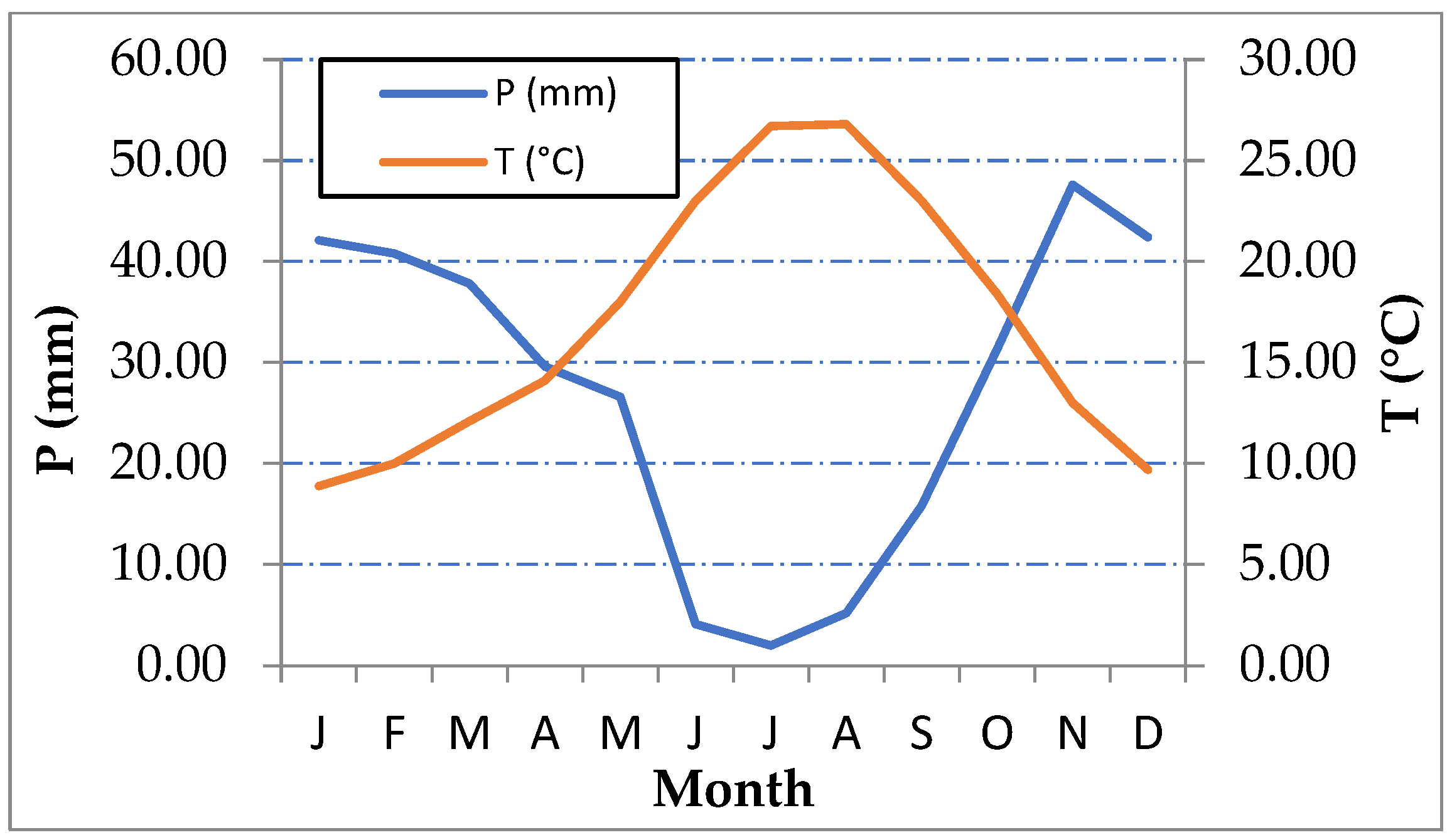
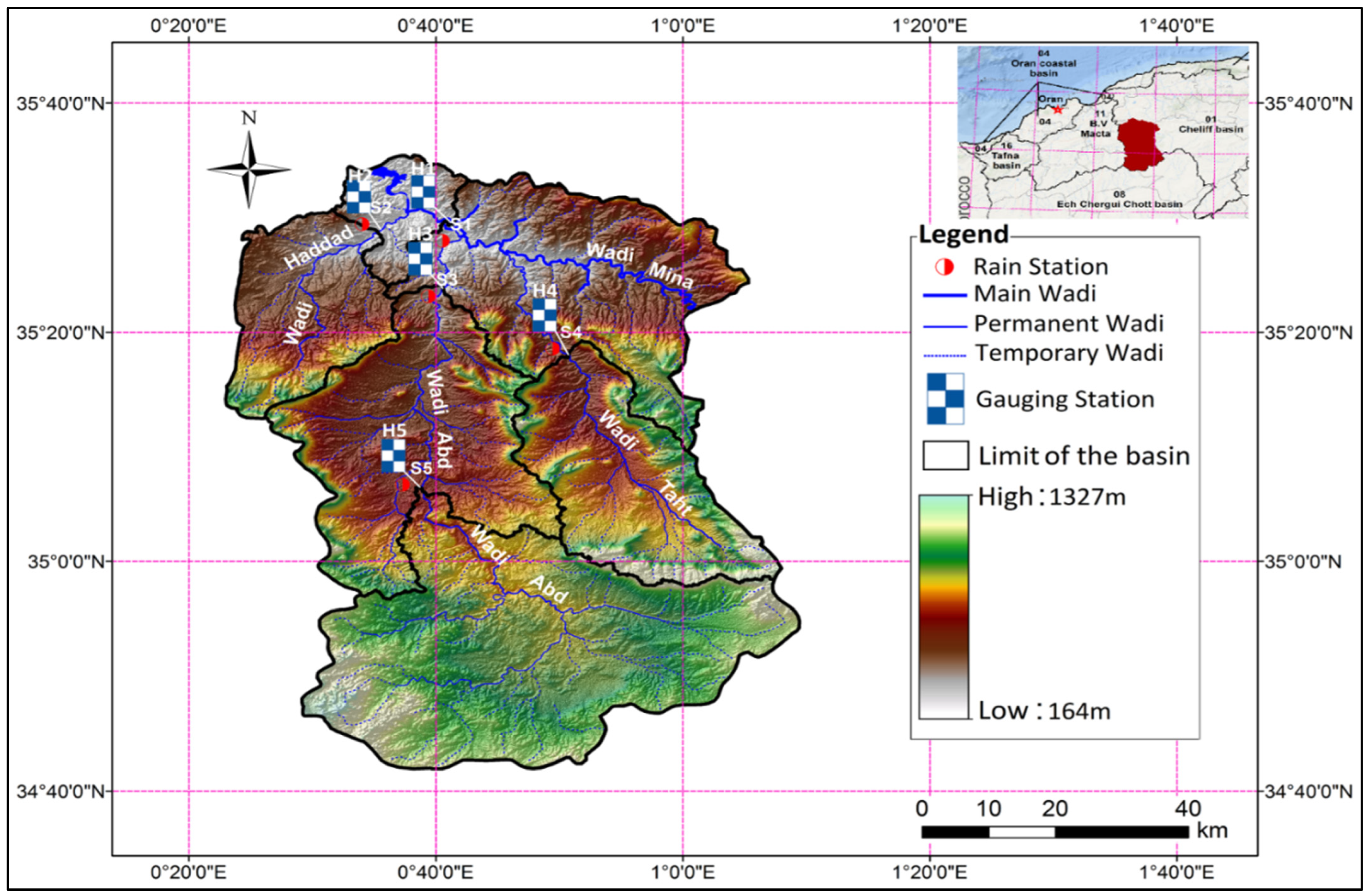
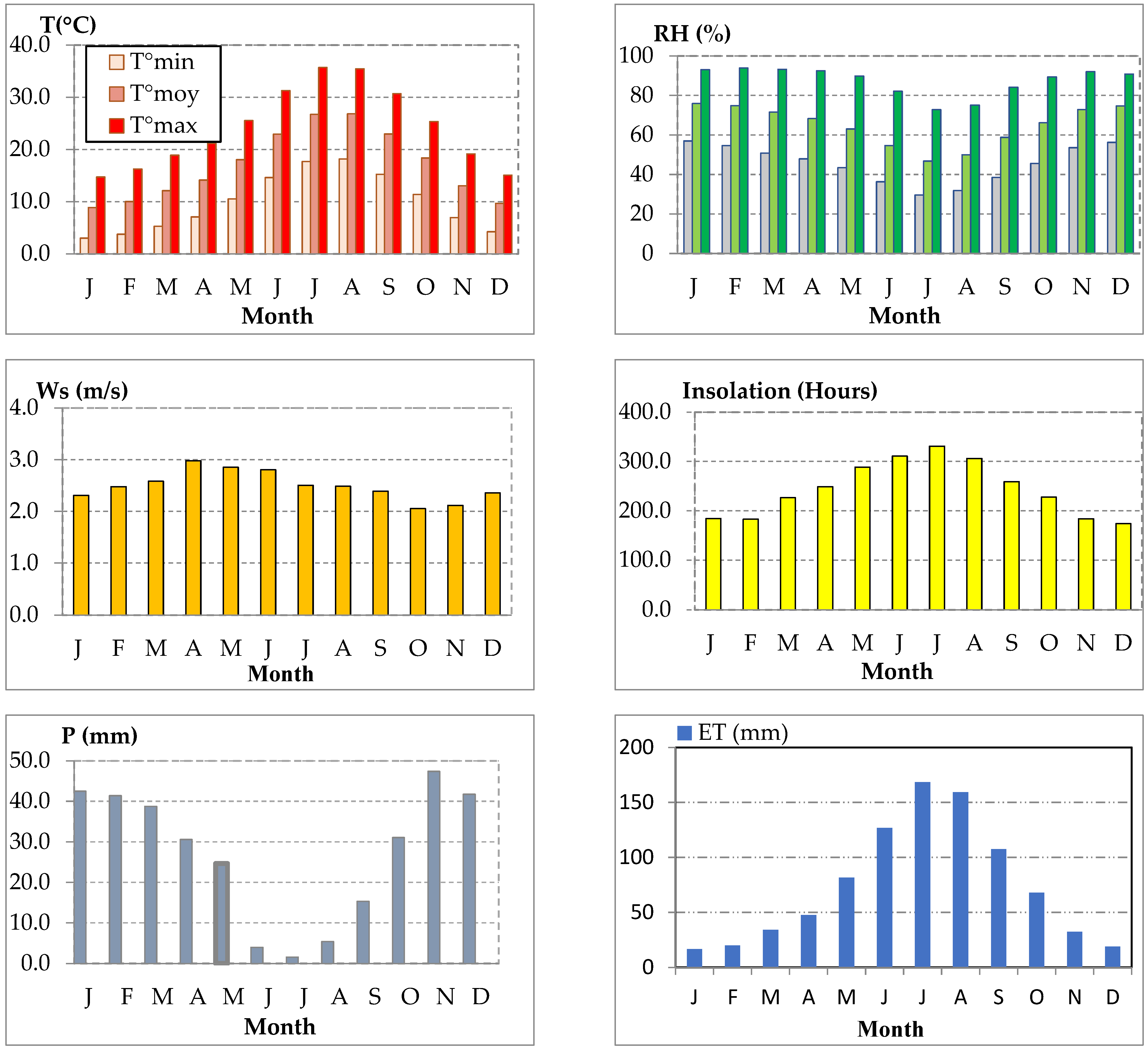
2. Study Area Description
3. Material and Methods
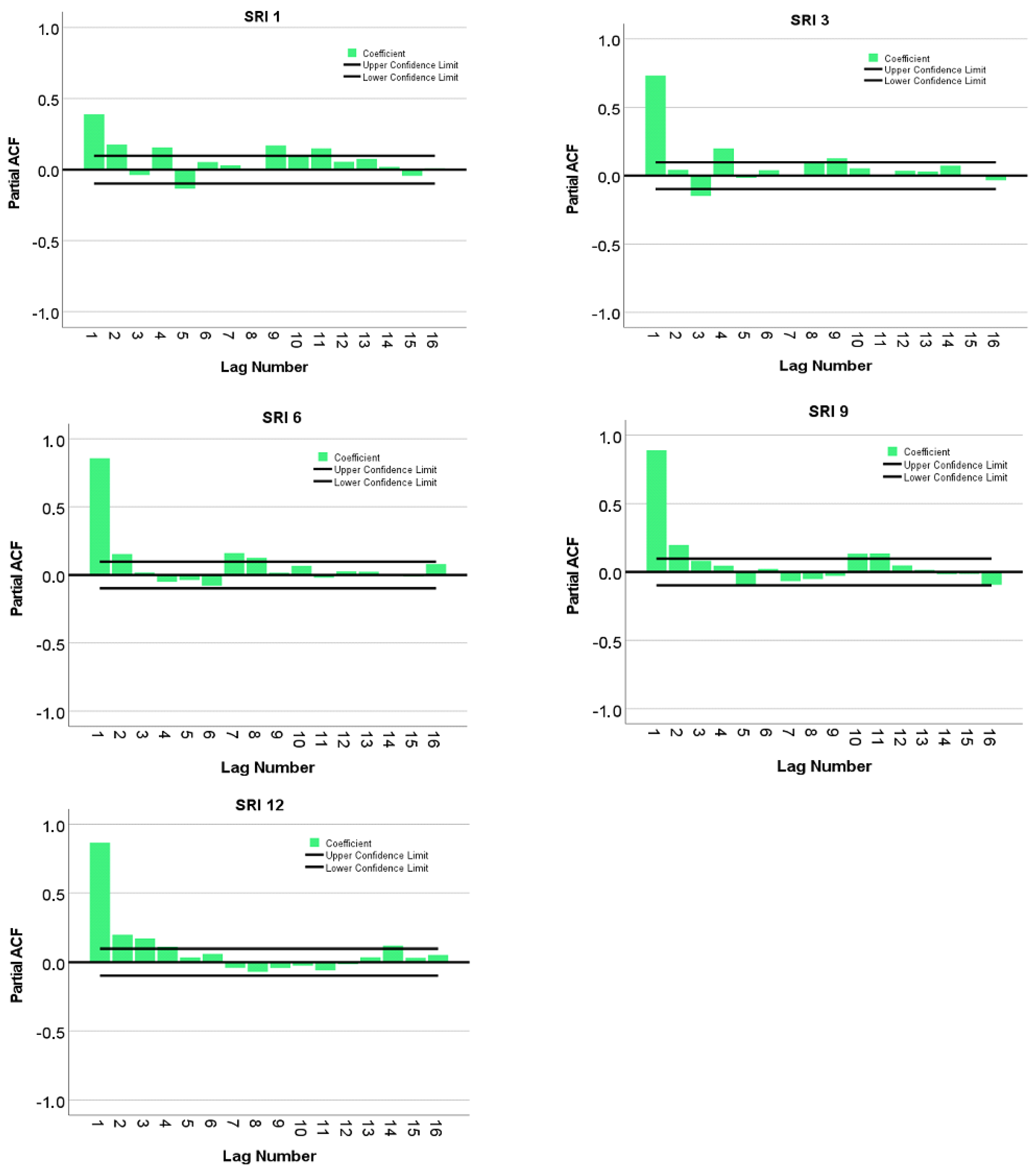
3.1. SRI
3.2. Extreme Learning Machine
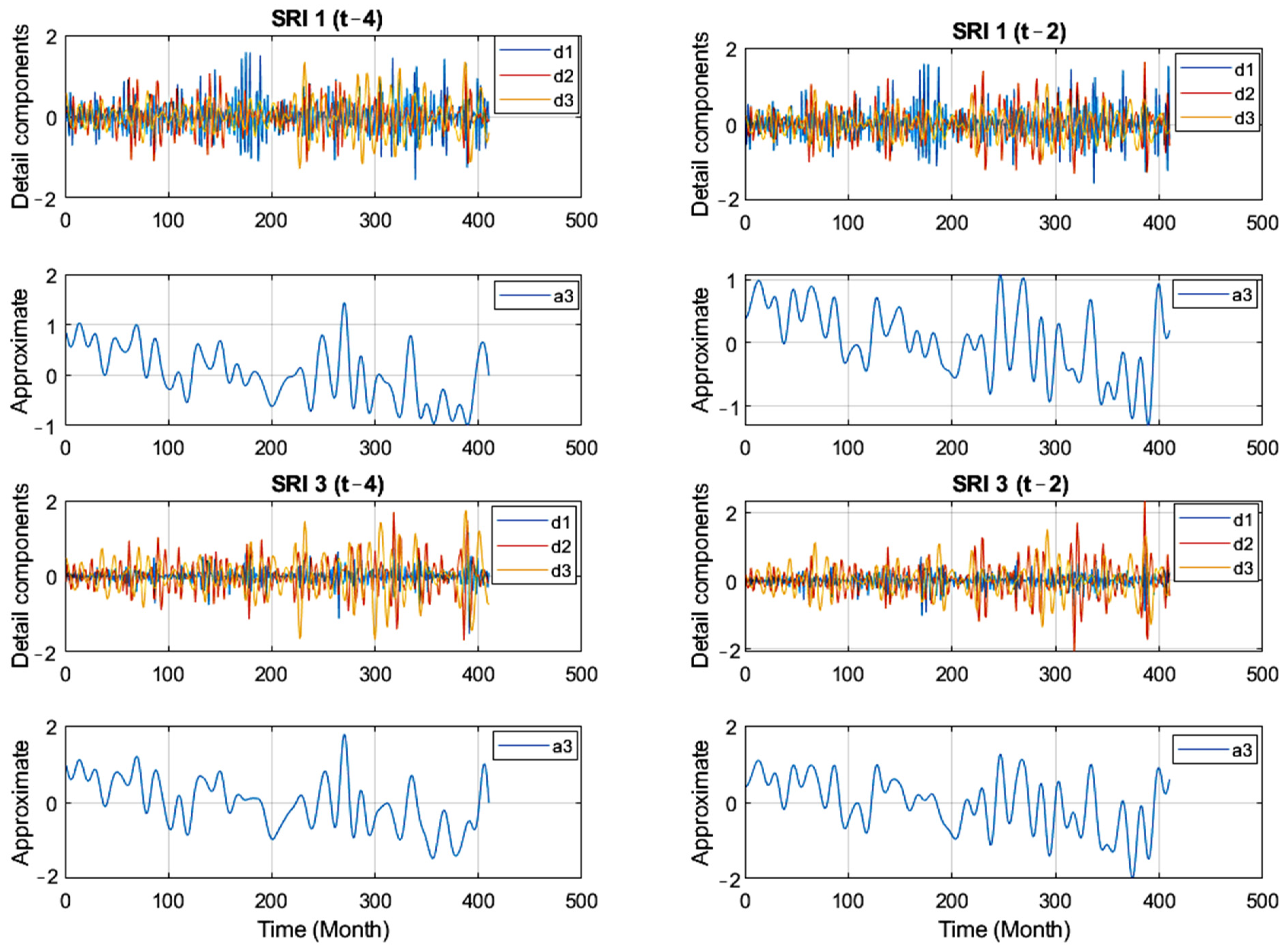
3.3. Wavelet Transform
3.4. Choosing the Approach of the Input Parameters
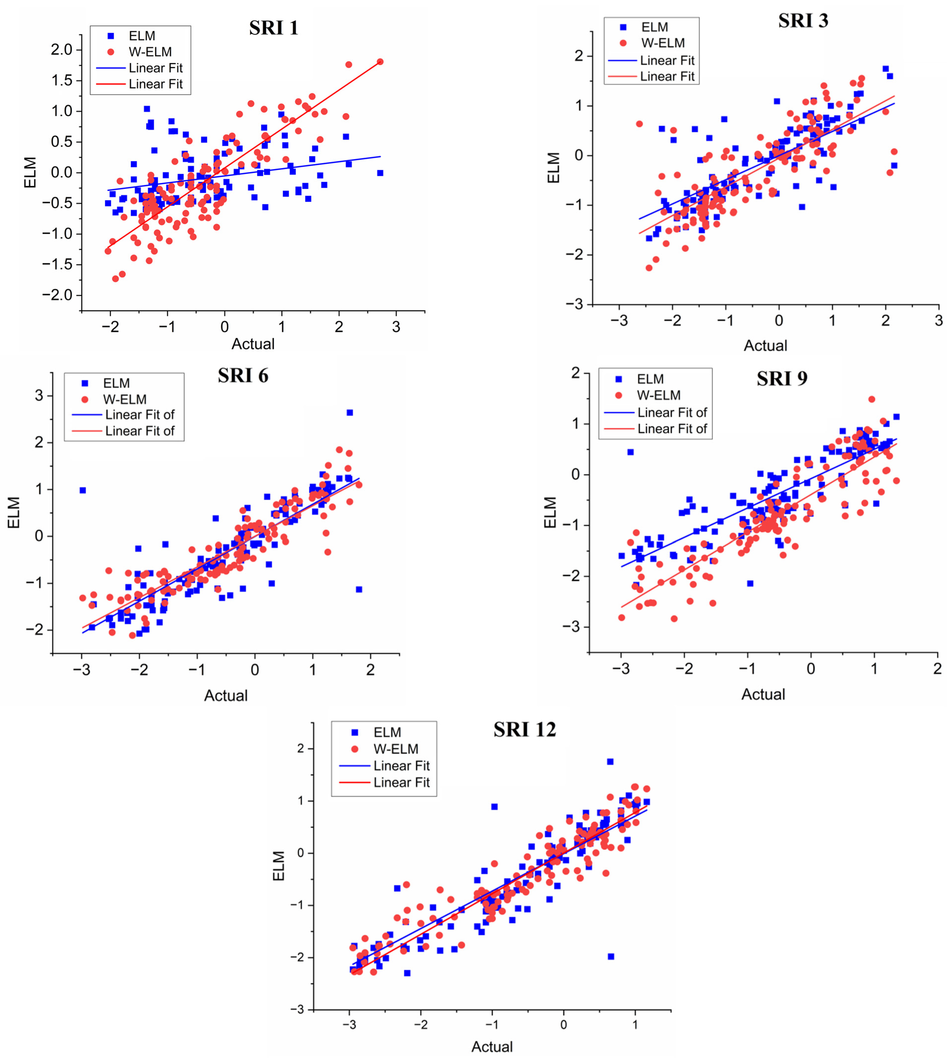
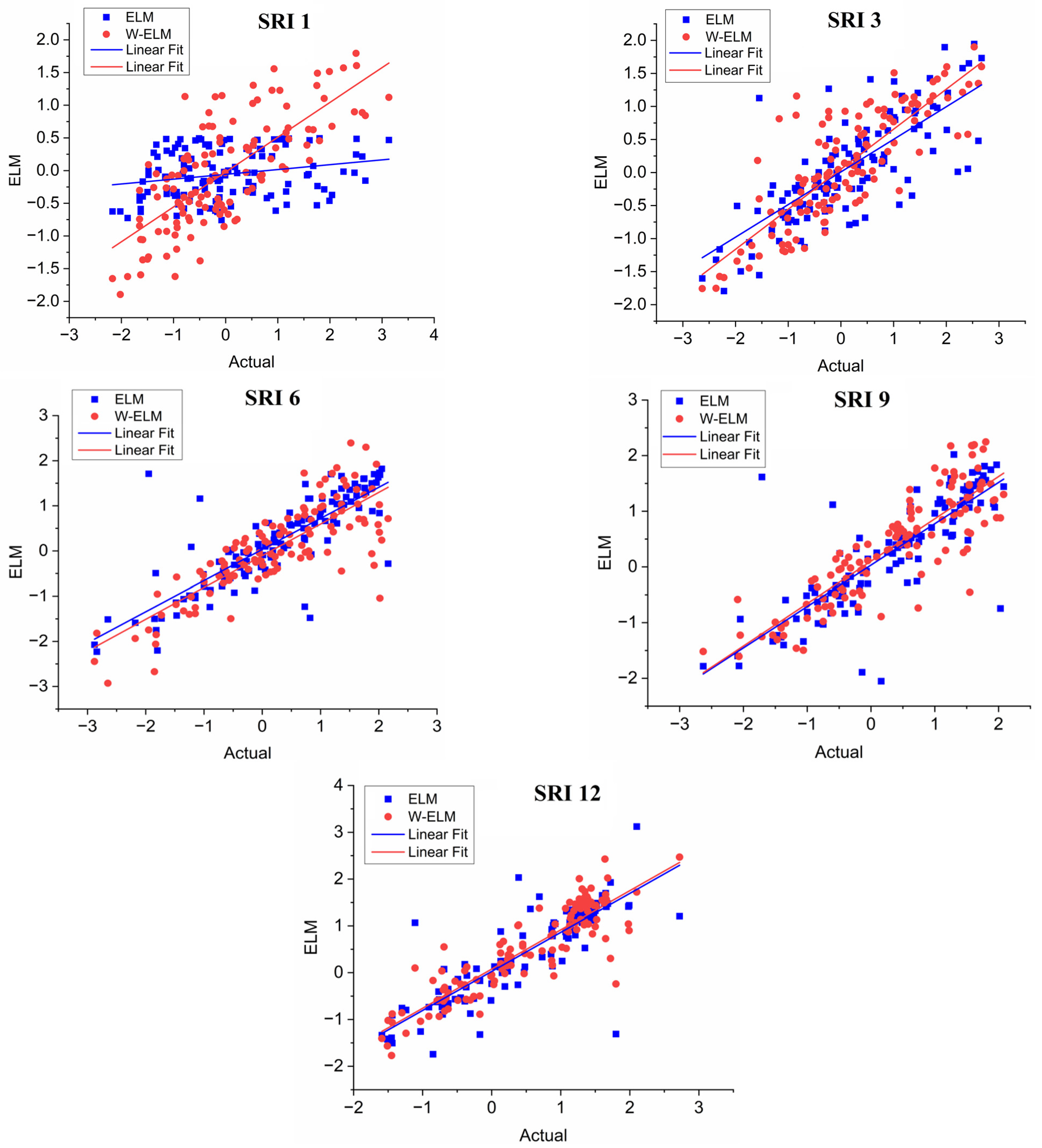
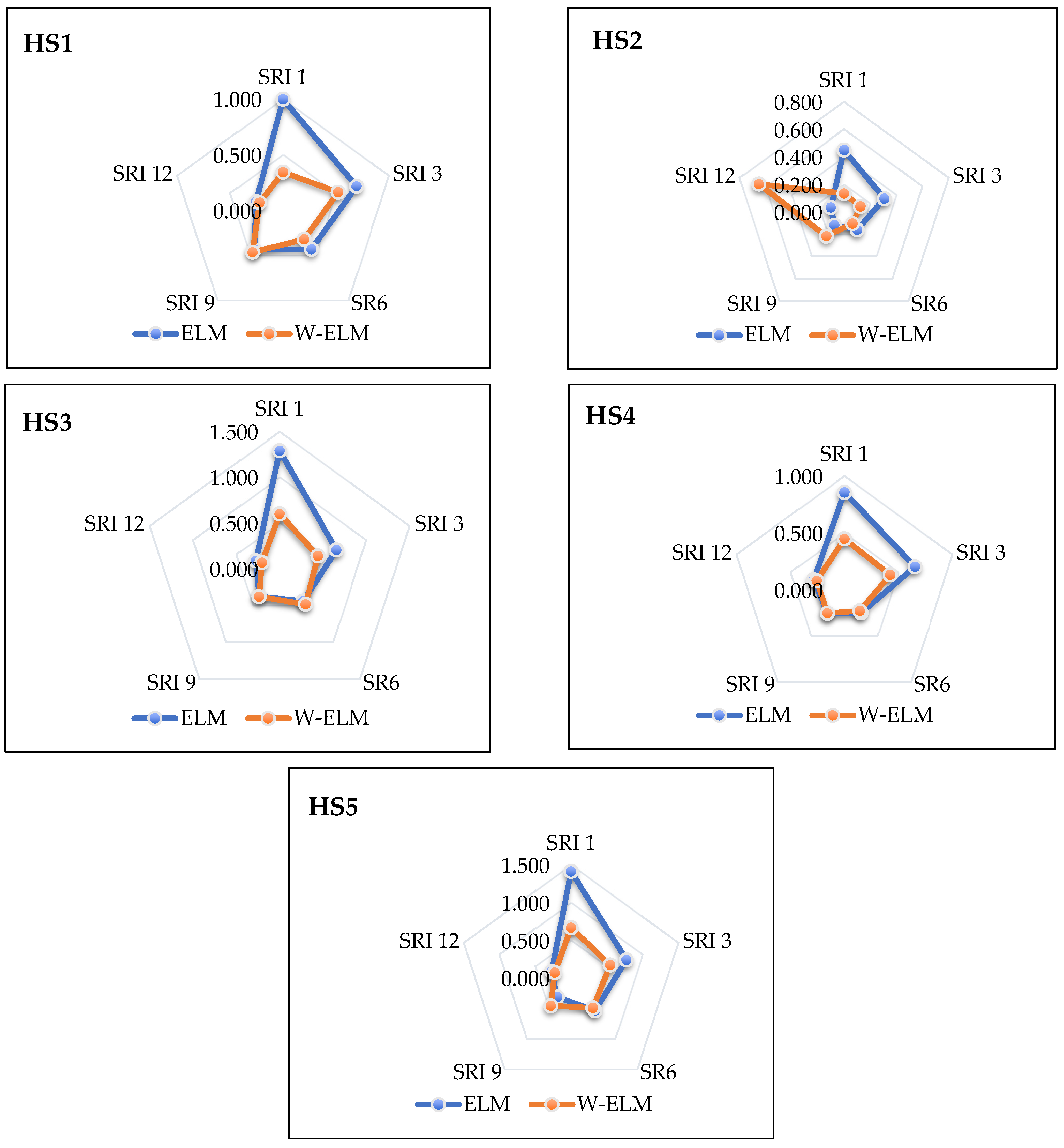
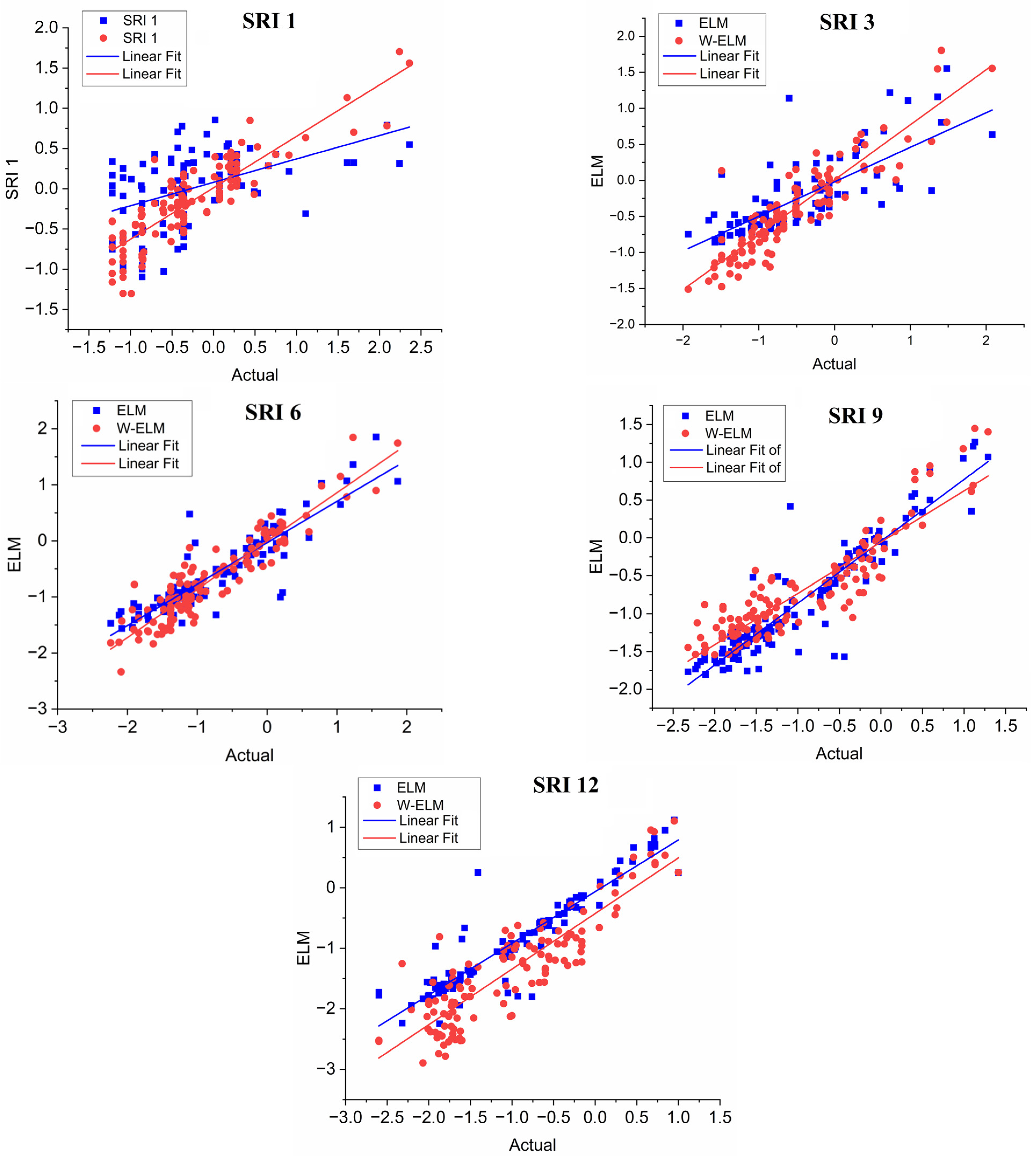
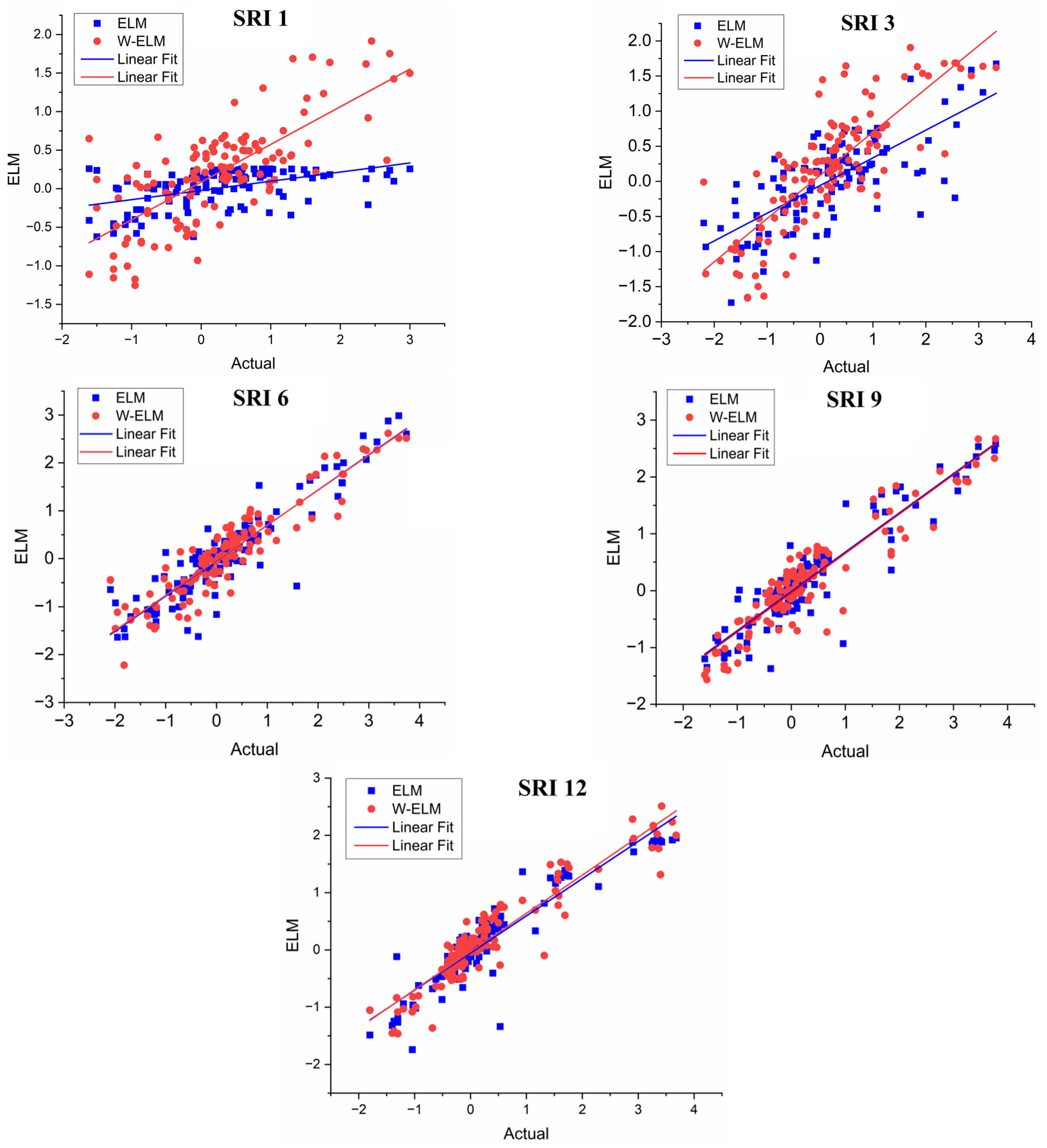
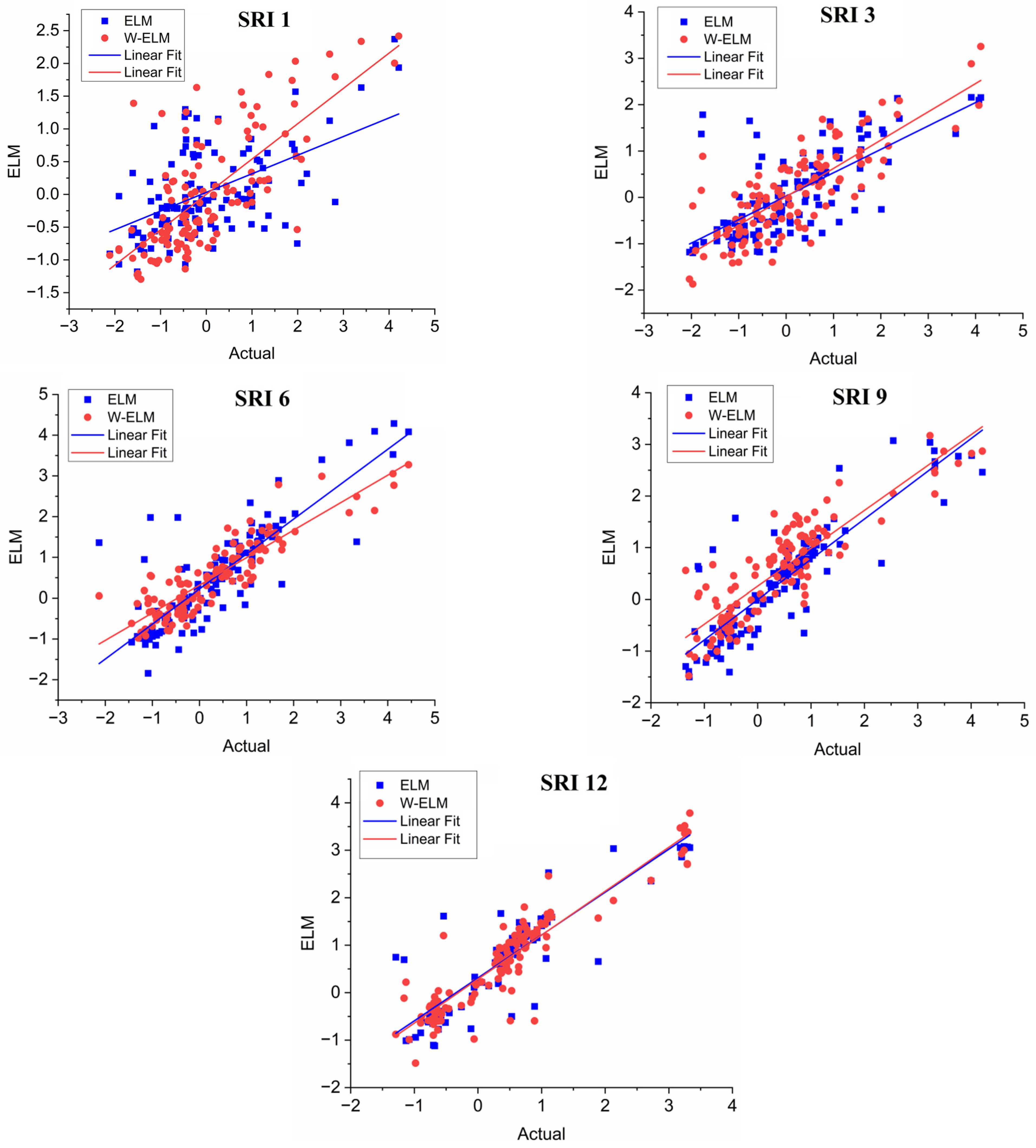
4. Results
5. Discussion
6. Conclusions
Author Contributions
Funding
Institutional Review Board Statement
Informed Consent Statement
Data Availability Statement
Conflicts of Interest
References
- Danandeh Mehr, A.; Rikhtehgar Ghiasi, A.; Yaseen, Z.M.; Sorman, A.U.; Abualigah, Ü.L. A novel intelligent deep learning predictive model for meteorological drought forecasting. J. Ambient Intell. Humaniz. Comput. 2022, 4, 85–97. [Google Scholar] [CrossRef]
- Khan, N.; Sachindra, D.A.; Shahid, S.; Ahmed, K.; Shiru, M.S.; Nawaz, N. Prediction of droughts over Pakistan using machine learning algorithms. Adv. Water Resour. 2020, 139, 103562. [Google Scholar] [CrossRef]
- Hao, Z.; Singh, V.P.; Xia, Y. Seasonal drought prediction: Advances, challenges, and future prospects. Rev. Geophys. 2018, 56, 108–141. [Google Scholar] [CrossRef]
- Durbach, I.; Merven, B.; McCall, B. Expert elicitation of autocorrelated time series with application to e3 (energy-environment-economic) forecasting models. Environ. Model. Softw. 2017, 88, 93–105. [Google Scholar] [CrossRef]
- Adnan, R.M.; Mostafa, R.R.; Islam, A.R.M.T.; Kisi, O.; Kuriqi, A.; Heddam, S. Estimating reference evapotranspiration using hybrid adaptive fuzzy inferencing coupled with heuristic algorithms. Comput. Electron. Agric. 2021, 191, 106541. [Google Scholar] [CrossRef]
- Azizi, E.; Tavakoli, M.; Karimi, H.; Faramarzi, M. Evaluating the efficiency of the neural network to other methods in predicting drought in arid and semi-arid regions of western Iran. Arab. J. Geosci. 2019, 12, 489. [Google Scholar] [CrossRef]
- Heim, R.R., Jr. A review of twentieth-century drought indices used in the United States. Bull. Am. Meteorol. Soc. 2002, 83, 1149–1166. [Google Scholar] [CrossRef]
- Ahmadalipour, A.; Moradkhani, H.; Demirel, M.C. A comparative assessment of projected meteorological and hydrological droughts: Elucidating the role of temperature. J. Hydrol. 2017, 553, 785–797. [Google Scholar] [CrossRef]
- Mishra, A.K.; Singh, V.P. Drought modeling—A review. J. Hydrol. 2011, 403, 157–175. [Google Scholar] [CrossRef]
- Jain, V.K.; Pandey, R.P.; Jain, M.K.; Byun, H.R. Comparison of drought indices for appraisal of drought characteristics in the Ken River Basin. Weather Clim. Extrem. 2015, 8, 1–11. [Google Scholar] [CrossRef]
- Kim, T.W.; Jehanzaib, M. Drought risk analysis, forecasting and assessment under climate change. Water 2020, 12, 1862. [Google Scholar] [CrossRef]
- Jehanzaib, M.; Bilal Idrees, M.; Kim, D.; Kim, T.W. Comprehensive evaluation of machine learning techniques for hydrological drought forecasting. J. Irrig. Drain. Eng. 2021, 147, 04021022. [Google Scholar] [CrossRef]
- Ali, M.; Ghaith, M.; Wagdy, A.; Helmi, A.M. Development of a new multivariate composite drought index for the Blue Nile River Basin. Water 2022, 14, 886. [Google Scholar] [CrossRef]
- Liang, G.; Panahi, F.; Ahmed, A.N.; Ehteram, M.; Band, S.S.; Elshafie, A. Predicting municipal solid waste using a coupled artificial neural network with archimedes optimisation algorithm and socioeconomic components. J. Clean. Prod. 2021, 315, 128039. [Google Scholar] [CrossRef]
- Dikshit, A.; Pradhan, B.; Alamri, A.M. Temporal hydrological drought index forecasting for New South Wales, Australia using machine learning approaches. Atmosphere 2020, 11, 585. [Google Scholar] [CrossRef]
- Sattar, M.N.; Jehanzaib, M.; Kim, J.E.; Kwon, H.H.; Kim, T.W. Application of the hidden Markov Bayesian classifier and propagation concept for probabilistic assessment of meteorological and hydrological droughts in South Korea. Atmosphere 2020, 11, 1000. [Google Scholar] [CrossRef]
- Nabipour, N.; Dehghani, M.; Mosavi, A.; Shamshirband, S. Short-term hydrological drought forecasting based on different nature-inspired optimization algorithms hybridized with artificial neural networks. IEEE Access 2020, 8, 15210–15222. [Google Scholar] [CrossRef]
- Habibi, B.; Meddi, M.; Torfs, P.J.; Remaoun, M.; Van Lanen, H.A. Characterisation and prediction of meteorological drought using stochastic models in the semi-arid Chéliff–Zahrez basin (Algeria). J. Hydrol. Reg. Stud. 2018, 16, 15–31. [Google Scholar] [CrossRef]
- Achite, M.; Wałęga, A.; Toubal, A.K.; Mansour, H.; Krakauer, N. Spatiotemporal characteristics and trends of meteorological droughts in the Wadi Mina Basin, Northwest Algeria. Water 2021, 13, 3103. [Google Scholar] [CrossRef]
- Achite, M.; Jehanzaib, M.; Elshaboury, N.; Kim, T.W. Evaluation of machine learning techniques for hydrological drought modeling: A case study of the Wadi Ouahrane Basin in Algeria. Water 2022, 14, 431. [Google Scholar] [CrossRef]
- Achite, M.; Banadkooki, F.B.; Ehteram, M.; Bouharira, A.; Ahmed, A.N.; Elshafie, A. Exploring Bayesian model averaging with multiple ANNs for meteorological drought forecasts. Stoch. Environ. Res. Risk Assess 2022, 36, 1835–1860. [Google Scholar] [CrossRef]
- Achite, M.; Touaibia, B. Sécheresse et gestion des ressources en eau dans le bassin versant de la Mina. In Proceedings of the International Conference on Water and Environment, Sidi Fredj, Algeria, 30–31 January 2007; Volume 30. [Google Scholar]
- Kumar, A.; Gosling, S.N.; Johnson, M.F.; Jones, M.D.; Zaherpour, J.; Kumar, R.; Leng, G.; Schmied, H.M.; Kupzig, J.; Breuer, L.; et al. Multi-model evaluation of catchment-and global-scale hydrological model simulations of drought characteristics across eight large river catchments. Adv. Water Resour. 2022, 165, 104212. [Google Scholar] [CrossRef]
- McKee, T.B.; Doesken, N.J.; Kleist, J. The relationship of drought frequency and duration to time scales. In Proceedings of the 8th Conference on Applied Climatology, Anaheim, CA, USA, 17–22 January 1993; Volume 17, pp. 179–183. [Google Scholar]
- Huang, G.B.; Zhu, Q.Y.; Siew, C.K. Extreme learning machine: Theory and applications. Neurocomputing 2006, 70, 489–501. [Google Scholar] [CrossRef]
- Acharya, N.; Shrivastava, N.A.; Panigrahi, B.; Mohanty, U. Development of an artificial neural network based multi-model ensemble to estimate the northeast monsoon rainfall over south peninsular India: An application of extreme learning machine. Clim. Dyn. 2013, 43, 1303–1310. [Google Scholar] [CrossRef]
- Rajesh, R.; Prakash, J.S. Extreme learning machines—A review and state of-the-art. Int. J. Wisdom Based Comput. 2011, 1, 35–49. [Google Scholar]
- Deo, R.C.; Şahin, M. Application of the extreme learning machine algorithm for the prediction of monthly effective drought index in eastern Australia. Atmos. Res. 2015, 153, 512–525. [Google Scholar] [CrossRef]
- Şahin, M. Modelling of air temperature using remote sensing and artificial neural network in Turkey. Adv. Space Res. 2012, 50, 973–985. [Google Scholar] [CrossRef]
- Şahin, M.; Kaya, Y.; Uyar, M.; Yıldırım, S. Application of extreme learning machine for estimating solar radiation from satellite data. Int. J. Energy Res. 2014, 38, 205–212. [Google Scholar] [CrossRef]
- Huang, G.B. Learning capability and storage capacity of two-hidden layer feedforward networks. IEEE Trans. Neural. Netw. 2003, 14, 274–281. [Google Scholar] [CrossRef]
- Maheswaran, R.; Khosa, R. Comparative study of different wavelets for hydrologic forecasting. Comput. Geosci. 2012, 46, 284–295. [Google Scholar] [CrossRef]
- Sang, Y.F. A review on the applications of Wavelet transform in hydrology time series analysis. Atmos. Res. 2013, 122, 8–15. [Google Scholar] [CrossRef]
- Daubechies, I. The wavelet transform, time-frequency localization and signal analysis. IEEE Trans. Inf. Theory 1990, 36, 961–1005. [Google Scholar] [CrossRef]
- Schneiders, M.G.E. Wavelets in Control Engineering. Master’s Thesis, Eindhoven University of Technology, Eindhoven, The Netherlands, 2001; p. 38. [Google Scholar]
- Ahmadi, F.; Mehdizadeh, S.; Mohammadi, B. Development of bio-inspired-and wavelet-based hybrid models for reconnaissance drought index modeling. Water Resour. Manag. 2021, 35, 4127–4147. [Google Scholar] [CrossRef]
- Mallat, S.G. A theory for multi resolution signal decomposition: The wavelet representation. IEEE Trans. Pattern Anal. Mach. Intel. 1989, 11, 674–693. [Google Scholar] [CrossRef]
- Sun, Z.; Chang, C. Structural damage assessment based on wavelet packet transform. J. Struct. Eng. 2002, 128, 1354–1361. [Google Scholar] [CrossRef]
- Katipoğlu, O.M. Combining discrete wavelet decomposition with soft computing techniques to predict monthly evapotranspiration in semi-arid Hakkâri province, Türkiye. Environ. Sci. Pollut. Res. 2023, 30, 44043–44066. [Google Scholar] [CrossRef] [PubMed]
- Tiwari, M.K.; Chatterjee, C. Development of an accurate and reliable hourly flood forecasting model using Wavelet–bootstrap–ANN (WBANN) hybrid approach. J. Hydrol. 2010, 394, 458–470. [Google Scholar] [CrossRef]
- Katipoğlu, O.M. Prediction of streamflow drought index for short-term hydrological drought in the semi-arid Yesilirmak Basin using Wavelet transform and artificial intelligence techniques. Sustainability 2023, 15, 1109. [Google Scholar] [CrossRef]


| ID | Name | Elevation (m) | Basin Area (km2) | Latitude | Longitude | |
|---|---|---|---|---|---|---|
| H1 | 013402 | Oued Abtal | 210 | 4126 | 35°29′26.28″ N | 0°41′00.49″ E |
| H2 | 013401 | Sidi Abdelkader Djillali | 241 | 480 | 35°28′46.05″ N | 0°35′19.99″ E |
| H3 | 013302 | Ain Hammara | 285 | 2480 | 35°23′50.09″ N | 0°40′33.19″ E |
| H4 | 013001 | Kef Mehboula | 502 | 680 | 35°18′05.21″ N | 0°50′47.89″ E |
| H5 | 013301 | Takhmaret | 634 | 1553 | 35°06′20.08″ N | 0°38′46.54″ E |
| HS1 | J | F | M | A | M | J | J | A | S | O | N | D | Ann. |
| Min (m3/s) | 2.051 | 2.517 | 2.677 | 1.897 | 2.245 | 0.925 | 0.912 | 0.845 | 1.780 | 3.494 | 1.975 | 1.531 | 1.904 |
| Max (m3/s) | 1.630 | 2.679 | 3.080 | 2.518 | 3.053 | 1.414 | 1.654 | 1.694 | 2.362 | 5.044 | 2.700 | 1.635 | 0.975 |
| Mean (m3/s) | 2.051 | 2.517 | 2.677 | 1.897 | 2.245 | 0.925 | 0.912 | 0.845 | 1.780 | 3.494 | 1.975 | 1.531 | 1.904 |
| SD (m3/s) | 1.630 | 2.679 | 3.080 | 2.518 | 3.053 | 1.414 | 1.654 | 1.694 | 2.362 | 5.044 | 2.700 | 1.635 | 0.975 |
| Kurtosis | −1.000 | 1.695 | 1.909 | 6.498 | 3.290 | 0.816 | 3.586 | 5.509 | 5.676 | 12.940 | 2.554 | 2.690 | −1.312 |
| Skewness | 0.497 | 1.447 | 1.471 | 2.301 | 1.836 | 1.446 | 2.007 | 2.404 | 2.202 | 3.130 | 1.813 | 1.695 | −0.077 |
| CV | 79.452 | 106.427 | 115.074 | 132.752 | 135.951 | 152.785 | 181.393 | 200.400 | 132.640 | 144.354 | 136.715 | 106.772 | 51.193 |
| HS2 | J | F | M | A | M | J | J | A | S | O | N | D | Ann. |
| Min (m3/s) | 0.000 | 0.000 | 0.000 | 0.000 | 0.000 | 0.000 | 0.000 | 0.000 | 0.000 | 0.000 | 0.000 | 0.000 | 0.001 |
| Max (m3/s) | 1.094 | 1.056 | 4.200 | 0.624 | 0.599 | 0.450 | 2.112 | 0.292 | 0.856 | 1.619 | 1.628 | 0.737 | 0.492 |
| Mean (m3/s) | 0.214 | 0.223 | 0.337 | 0.112 | 0.084 | 0.056 | 0.113 | 0.027 | 0.091 | 0.256 | 0.227 | 0.167 | 0.159 |
| SD (m3/s) | 0.251 | 0.268 | 0.723 | 0.158 | 0.127 | 0.110 | 0.416 | 0.070 | 0.171 | 0.414 | 0.347 | 0.182 | 0.130 |
| Kurtosis | 4.697 | 1.421 | 24.475 | 3.910 | 7.172 | 5.530 | 18.084 | 10.613 | 11.179 | 4.871 | 7.488 | 2.769 | −0.173 |
| Skewness | 1.941 | 1.353 | 4.628 | 2.005 | 2.454 | 2.449 | 4.271 | 3.331 | 3.060 | 2.216 | 2.582 | 1.664 | 0.766 |
| CV | 116.87 | 119.96 | 214.69 | 141.31 | 151.66 | 197.68 | 369.04 | 257.85 | 188.04 | 161.58 | 152.78 | 109.04 | 81.89 |
| HS3 | J | F | M | A | M | J | J | A | S | O | N | D | Ann. |
| Min (m3/s) | 0.408 | 0.178 | 0.096 | 0.030 | 0.006 | 0.000 | 0.000 | 0.000 | 0.017 | 0.064 | 0.122 | 0.318 | 0.370 |
| Max (m3/s) | 3.700 | 5.409 | 8.058 | 3.269 | 8.417 | 2.758 | 3.527 | 11.172 | 10.010 | 19.435 | 6.713 | 2.874 | 2.541 |
| Mean (m3/s) | 1.211 | 1.325 | 1.455 | 0.939 | 0.979 | 0.408 | 0.292 | 0.647 | 1.357 | 2.856 | 1.492 | 1.072 | 1.169 |
| SD (m3/s) | 0.839 | 1.195 | 1.645 | 0.822 | 1.857 | 0.547 | 0.607 | 1.869 | 2.025 | 4.098 | 1.613 | 0.652 | 0.539 |
| Kurtosis | 2.667 | 3.961 | 7.031 | 0.917 | 13.191 | 9.248 | 24.151 | 30.908 | 9.796 | 7.398 | 2.960 | 0.634 | 0.492 |
| Skewness | 1.730 | 1.956 | 2.448 | 1.234 | 3.677 | 2.676 | 4.604 | 5.429 | 2.955 | 2.534 | 1.902 | 1.145 | 0.829 |
| CV | 69.325 | 90.178 | 113.042 | 87.520 | 189.731 | 133.982 | 207.598 | 288.936 | 149.268 | 143.481 | 108.142 | 60.800 | 46.093 |
| HS4 | J | F | M | A | M | J | J | A | S | O | N | D | Ann. |
| Min (m3/s) | 0.010 | 0.008 | 0.004 | 0.000 | 0.000 | 0.000 | 0.000 | 0.000 | 0.000 | 0.000 | 0.006 | 0.006 | 0.022 |
| Max (m3/s) | 3.150 | 2.750 | 2.641 | 2.200 | 3.369 | 0.800 | 0.223 | 1.219 | 1.921 | 3.500 | 2.600 | 3.200 | 1.194 |
| Mean (m3/s) | 0.447 | 0.468 | 0.465 | 0.283 | 0.305 | 0.116 | 0.030 | 0.088 | 0.292 | 0.511 | 0.398 | 0.398 | 0.317 |
| SD (m3/s) | 0.632 | 0.692 | 0.706 | 0.469 | 0.607 | 0.191 | 0.046 | 0.222 | 0.495 | 0.786 | 0.509 | 0.632 | 0.209 |
| Kurtosis | 9.108 | 4.274 | 3.504 | 8.924 | 19.140 | 5.651 | 8.173 | 20.473 | 3.305 | 5.367 | 9.337 | 11.537 | 8.080 |
| Skewness | 2.750 | 2.258 | 2.094 | 2.884 | 4.063 | 2.449 | 2.538 | 4.331 | 2.062 | 2.258 | 2.654 | 3.180 | 2.180 |
| CV | 141.414 | 147.886 | 151.765 | 165.434 | 198.901 | 164.933 | 152.445 | 253.629 | 169.243 | 153.735 | 128.027 | 158.846 | 65.888 |
| HS5 | J | F | M | A | M | J | J | A | S | O | N | D | Ann. |
| Min (m3/s) | 0.052 | 0.000 | 0.000 | 0.025 | 0.007 | 0.000 | 0.000 | 0.000 | 0.000 | 0.013 | 0.043 | 0.070 | 0.085 |
| Max (m3/s) | 2.119 | 2.720 | 4.646 | 2.694 | 17.954 | 14.463 | 12.810 | 10.711 | 8.698 | 9.634 | 2.375 | 2.110 | 4.281 |
| Mean (m3/s) | 0.475 | 0.527 | 0.594 | 0.443 | 1.205 | 0.583 | 0.465 | 0.500 | 1.162 | 1.877 | 0.483 | 0.408 | 0.727 |
| SD (m3/s) | 0.430 | 0.570 | 0.861 | 0.591 | 3.348 | 2.403 | 2.128 | 1.795 | 2.075 | 2.626 | 0.518 | 0.389 | 0.827 |
| Kurtosis | 7.675 | 6.565 | 14.565 | 7.032 | 18.845 | 34.494 | 35.172 | 32.301 | 7.511 | 2.154 | 5.821 | 10.125 | 11.321 |
| Skewness | 2.692 | 2.464 | 3.580 | 2.633 | 4.163 | 5.827 | 5.904 | 5.587 | 2.709 | 1.773 | 2.373 | 2.876 | 3.192 |
| CV | 90.675 | 108.131 | 145.009 | 133.426 | 277.900 | 412.475 | 457.964 | 358.748 | 178.650 | 139.894 | 107.163 | 95.295 | 113.758 |
| SRI Values | Drought Category | Probability (%) |
|---|---|---|
| ≥2.00 | Extremely wet | 2.3 |
| 1.50–1.99 | Very wet | 4.4 |
| 1.00–1.49 | Moderate wet | 9.2 |
| −0.99–0.99 | Near normal | 68.2 |
| −1.00–−1.49 | Moderately drought | 9.2 |
| −1.50–−1.99 | Severely drought | 4.4 |
| ≤−2.00 | Extremely drought | 2.3 |
| SRI1 | SRI3 | SRI6 | SRI9 | SRI12 | |
|---|---|---|---|---|---|
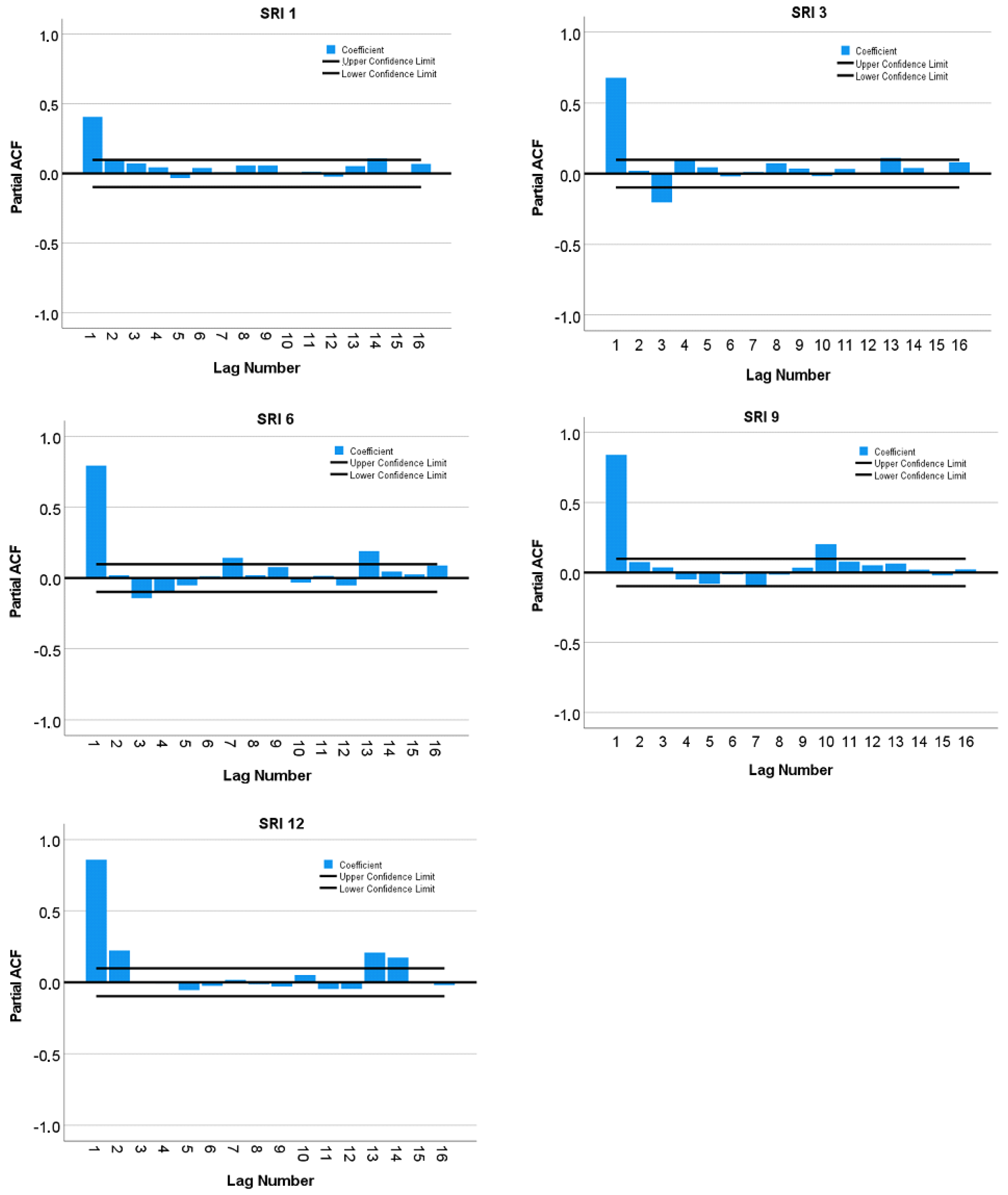
| HS1 | SRI1 (t-1) SRI1 (t-2) SRI1 (t-4) | SRI3 (t-1) SRI3 (t-4) | SRI6 (t-1) SRI6 (t-2) | SRI9 (t-1) SRI9 (t-10) | SRI12 (t-1) SRI12 (t-2) SRI12 (t-3) |
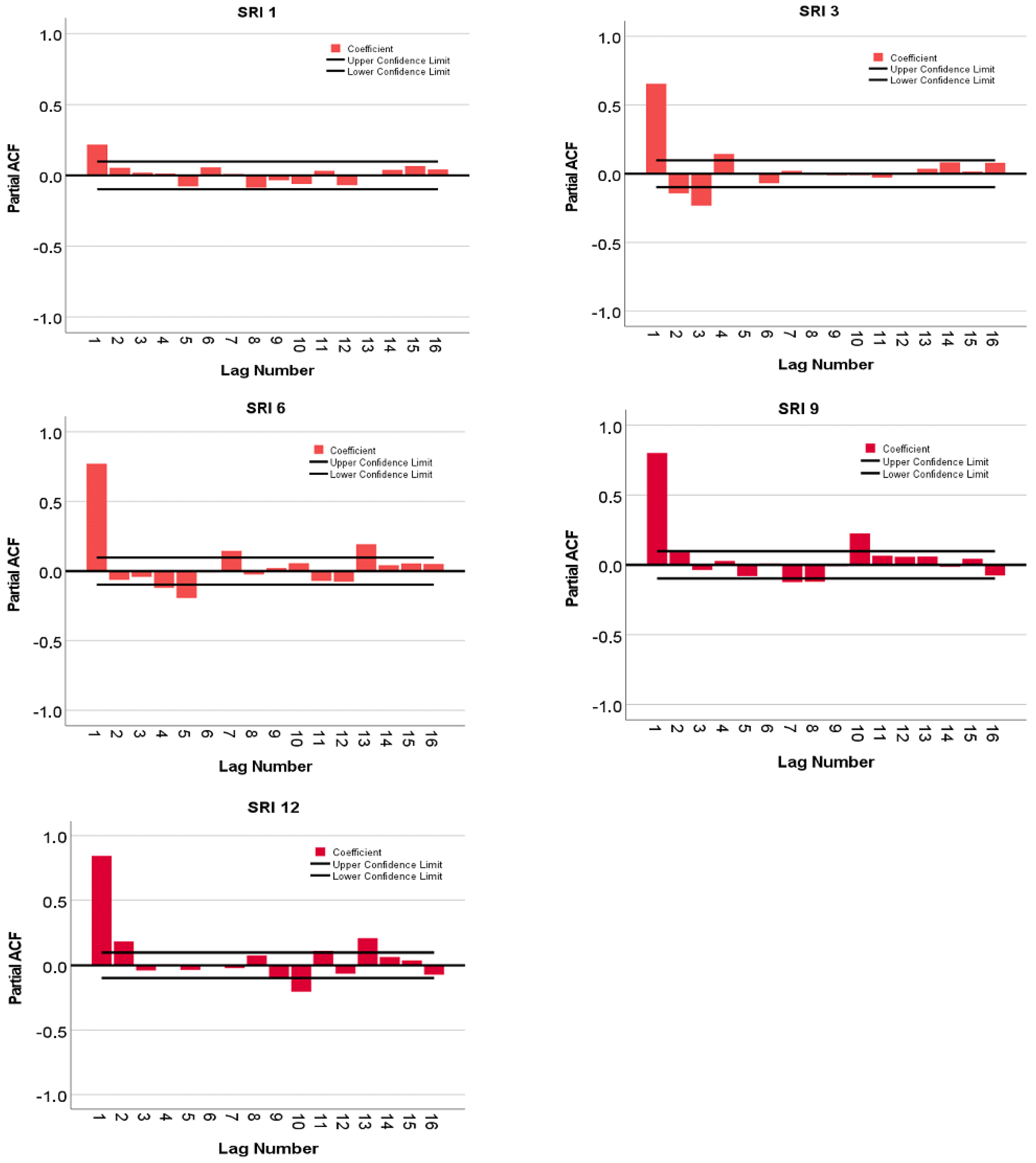
| HS2 | SRI1 (t-1) SRI1 (t-2) SRI1 (t-4) | SRI3 (t-1) SRI3 (t-4) | SRI6 (t-1) SRI6 (t-2) | SRI9 (t-1) SRI9 (t-2) | SRI12 (t-1) SRI12 (t-2) SRI12 (t-3) |
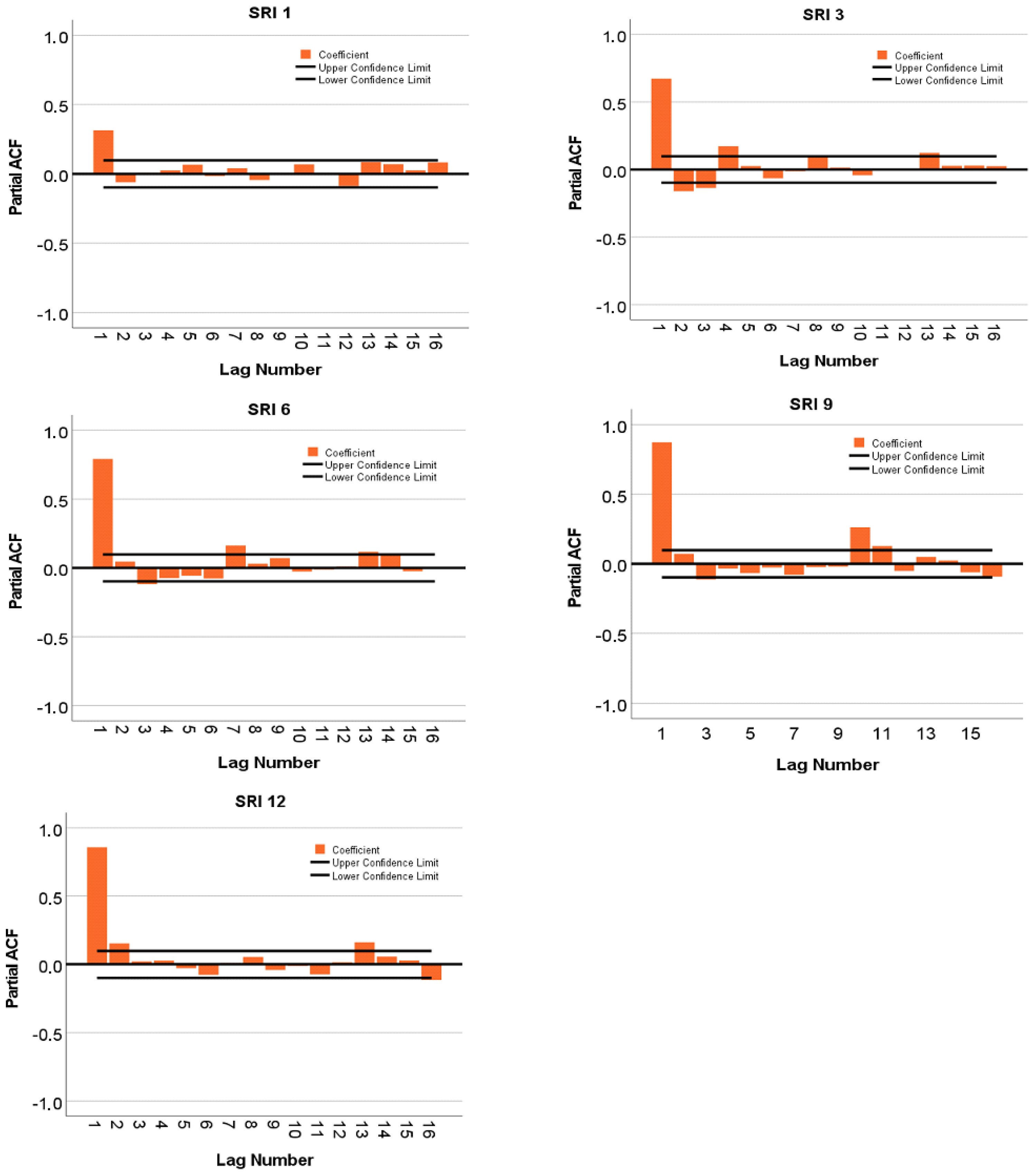
| HS3 | SRI1 (t-1) | SRI3 (t-1) | SRI6 (t-1) | SRI9 (t-1) SRI9 (t-10) | SRI12 (t-1) SRI12 (t-2) |
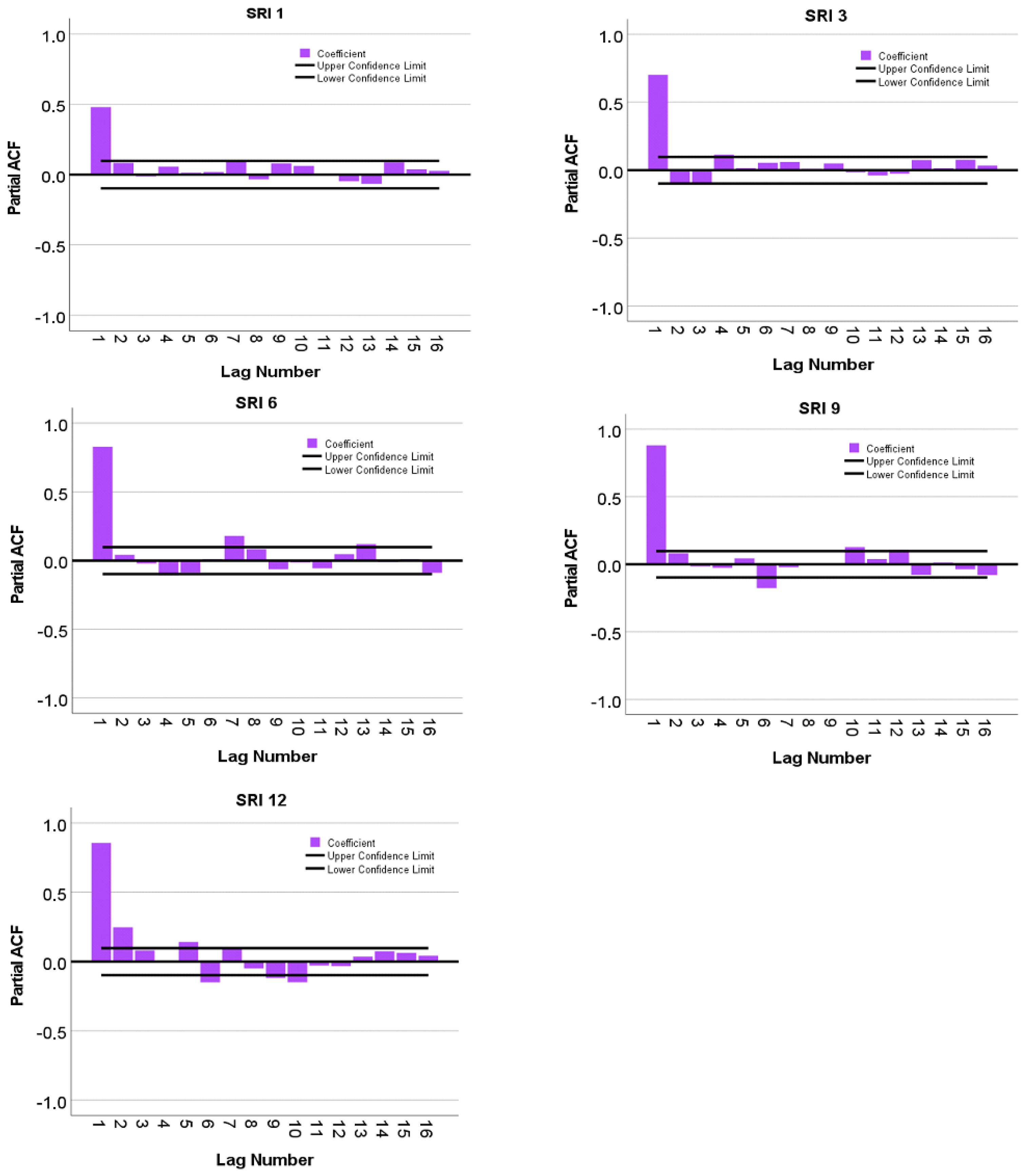
| HS4 | SRI1 (t-1) | SRI3 (t-1) SRI3 (t-4) | SRI6 (t-1) SRI6 (t-7) | SRI9 (t-1) SRI9 (t-10) | SRI12 (t-1) SRI12 (t-2) |
| HS5 | SRI1 (t-1) | SRI3 (t-1) | SRI6 (t-1) | SRI9 (t-1) SRI9 (t-7) | SRI12 (t-1) |
| HS1 | HS2 | HS3 | HS4 | HS5 | |||||||
|---|---|---|---|---|---|---|---|---|---|---|---|
| ELM | W-ELM | ELM | W-ELM | ELM | W-ELM | ELM | W-ELM | ELM | W-ELM | ||
| SRI 1 | R2 | 0.083 | 0.708 | 0.223 | 0.768 | 0.055 | 0.561 | 0.240 | 0.549 | 0.251 | 0.537 |
| MSE | 0.996 | 0.342 | 0.449 | 0.133 | 1.288 | 0.596 | 0.854 | 0.448 | 1.412 | 0.666 | |
| MAE | 0.801 | 0.470 | 0.500 | 0.281 | 0.919 | 0.630 | 0.685 | 0.512 | 0.928 | 0.615 | |
| SRI 3 | R2 | 0.500 | 0.610 | 0.565 | 0.804 | 0.520 | 0.683 | 0.534 | 0.664 | 0.490 | 0.640 |
| MSE | 0.695 | 0.521 | 0.309 | 0.126 | 0.655 | 0.443 | 0.654 | 0.424 | 0.773 | 0.547 | |
| MAE | 0.582 | 0.505 | 0.440 | 0.280 | 0.587 | 0.509 | 0.592 | 0.504 | 0.608 | 0.563 | |
| SR6 | R2 | 0.702 | 0.822 | 0.813 | 0.862 | 0.678 | 0.669 | 0.835 | 0.855 | 0.715 | 0.782 |
| MSE | 0.434 | 0.323 | 0.162 | 0.105 | 0.443 | 0.486 | 0.250 | 0.230 | 0.540 | 0.494 | |
| MAE | 0.404 | 0.416 | 0.303 | 0.247 | 0.409 | 0.495 | 0.350 | 0.349 | 0.436 | 0.502 | |
| SRI 9 | R2 | 0.712 | 0.794 | 0.865 | 0.811 | 0.687 | 0.741 | 0.855 | 0.861 | 0.769 | 0.766 |
| MSE | 0.438 | 0.467 | 0.119 | 0.219 | 0.381 | 0.384 | 0.255 | 0.255 | 0.314 | 0.459 | |
| MAE | 0.475 | 0.501 | 0.245 | 0.381 | 0.376 | 0.449 | 0.345 | 0.343 | 0.342 | 0.482 | |
| SRI 12 | R2 | 0.817 | 0.871 | 0.870 | 0.779 | 0.738 | 0.794 | 0.869 | 0.877 | 0.825 | 0.855 |
| MSE | 0.253 | 0.221 | 0.101 | 0.651 | 0.273 | 0.205 | 0.285 | 0.257 | 0.271 | 0.228 | |
| MAE | 0.309 | 0.349 | 0.191 | 0.640 | 0.305 | 0.322 | 0.307 | 0.318 | 0.293 | 0.318 | |
Disclaimer/Publisher’s Note: The statements, opinions and data contained in all publications are solely those of the individual author(s) and contributor(s) and not of MDPI and/or the editor(s). MDPI and/or the editor(s) disclaim responsibility for any injury to people or property resulting from any ideas, methods, instructions or products referred to in the content. |
© 2023 by the authors. Licensee MDPI, Basel, Switzerland. This article is an open access article distributed under the terms and conditions of the Creative Commons Attribution (CC BY) license (https://creativecommons.org/licenses/by/4.0/).
Share and Cite
Achite, M.; Katipoğlu, O.M.; Jehanzaib, M.; Elshaboury, N.; Kartal, V.; Ali, S. Hydrological Drought Prediction Based on Hybrid Extreme Learning Machine: Wadi Mina Basin Case Study, Algeria. Atmosphere 2023, 14, 1447. https://doi.org/10.3390/atmos14091447
Achite M, Katipoğlu OM, Jehanzaib M, Elshaboury N, Kartal V, Ali S. Hydrological Drought Prediction Based on Hybrid Extreme Learning Machine: Wadi Mina Basin Case Study, Algeria. Atmosphere. 2023; 14(9):1447. https://doi.org/10.3390/atmos14091447
Chicago/Turabian StyleAchite, Mohammed, Okan Mert Katipoğlu, Muhammad Jehanzaib, Nehal Elshaboury, Veysi Kartal, and Shoaib Ali. 2023. "Hydrological Drought Prediction Based on Hybrid Extreme Learning Machine: Wadi Mina Basin Case Study, Algeria" Atmosphere 14, no. 9: 1447. https://doi.org/10.3390/atmos14091447
APA StyleAchite, M., Katipoğlu, O. M., Jehanzaib, M., Elshaboury, N., Kartal, V., & Ali, S. (2023). Hydrological Drought Prediction Based on Hybrid Extreme Learning Machine: Wadi Mina Basin Case Study, Algeria. Atmosphere, 14(9), 1447. https://doi.org/10.3390/atmos14091447