Article

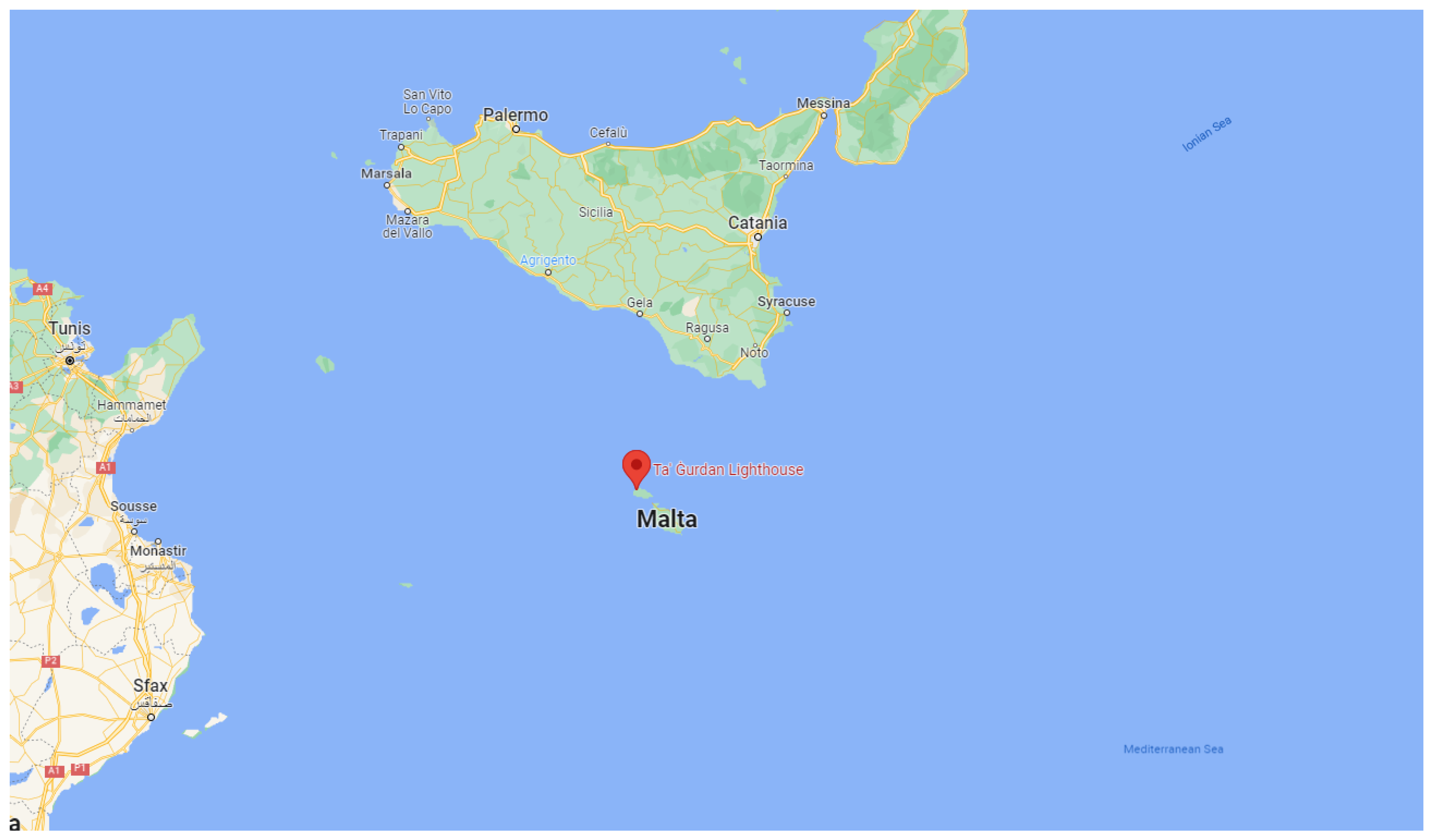
Long-Term Tropospheric Ozone Data Analysis 1997–2019 at Giordan Lighthouse, Gozo, Malta

1
Department of Chemistry, Josip Juraj Strossmayer University of Osijek, 31000 Osijek, Croatia
2
Department of Geosciences, University of Malta, 2080 Msida, Malta
*
Author to whom correspondence should be addressed.
Atmosphere 2023, 14(9), 1446; https://doi.org/10.3390/atmos14091446
Submission received: 19 July 2023 / Revised: 9 September 2023 / Accepted: 13 September 2023 / Published: 17 September 2023
(This article belongs to the Special Issue Airborne Measurements and Analyses of Trace Gases)

Abstract

:
Long-term data analysis of the hourly ozone volume fractions in the middle of the Mediterranean Seawas carried out covering a period of 22 years. It was noticed that the amount of ozone during this period very rarely exceeded the recommended upper limit value of 80 ppb and that the amount of tropospheric ozone in the area is rather low. Fourier data analysis shows the presence of only a seasonal cycle in ozone concentrations. Statistical analysis of the data is showing a slightly negative trend in ozone concentrations of −0.46 ± 0.08 ppb/year for average values and a slightly higher negative trend of −0.54 ± 0.11 ppb/year for the 95th percentile values. These results obtained through simple linear regression were confirmed using the more appropriate Mann–Kendall test. The possible quadratic trend was not observed for the whole series of data. Air mass trajectories were calculated for those days in the year with the highest pollution, indicating that during those days horizontal air transfer, in most cases, brings the air mass from the North and from Sicily in Southern Italy.

1. Introduction

For almost a century and especially after World War II, due to a large global population increase, air pollution problems have become of significant importance for the future of humankind. The everlasting negative impacts of various components in the air, especially those emitted by human activity, are of great concern. Therefore, continuous monitoring and analysis of data are of the greatest importance to improving air quality and the quality of life in general. As for the components of the air, the most widely recognised pollutants in the troposphere are various oxides (for example NOx), ground-level ozone, O3 and particulate matter (PM) [1,2,3,4,5,6].
Of those, tropospheric ozone is one of the most important. Unlike its stratospheric counterpart, which is of utmost importance for preserving terrestrial life forms [7], in the troposphere it is one of the most dangerous pollutants which causes tissue damage in both plants and animals, including humans [8,9,10]. Although not as important as carbon dioxide, ozone is also a greenhouse gas and its influence on the greenhouse effect cannot be omitted [11]. Its presence in the troposphere is caused by formation in photochemical reactions (about 90%) and by stratospheric intrusions or diffusion (about 10%) [12]. It can also be formed from lightning discharges during thunderstorms. Photochemical reactions that are essential for ozone production include primary pollutants as volatile organic compounds VOC and nitrogen oxides NOx [13,14]. Since diesel and heavy fuel oil engines are commonly used as a form of power for ships, and since Malta is located in the middle of the Mediterranean Sea on the major maritime transport routes, this area is extremely prone to pollution by nitrogen oxides [15] despite the low efficiency of NOx emitted by ship engines as the ozone precursors in the marine boundary layer [16,17]. That is in addition to typical Mediterranean meteorological conditions that include high insolation, anthropogenic, and biogenic ozone precursors concentrations, which all favour photochemical ozone production [18,19,20].
Meteorological conditions also have a large impact on ozone concentrations [21,22]. Wind speed and direction can influence a horizontal transfer; higher temperatures usually accompanied by higher insolation and humidity can also influence its deposition (i.e., loss of concentration in air) [23,24,25].
Giordan Lighthouse is located on one of the main maritime trade routes in Europe and the world. It also faces Sicily and its volcano, Mount Etna, which is the main natural source of particulate matter and gaseous atmospheric pollutants [26]. For a quality mathematical analysis of photochemical pollution, it is very useful to have a long-term data set, which is a fairly common way of analysing ozone trends [27]. Together with forecasting methods [28], long-term data analyses gives the best insight into the real situation. By obtaining data in the two-decade time span available, it is now possible to obtain a real insight into the situation in this area. It is known that global tropospheric ozone concentrations in the background increase by an annual rate of around 2% [29]. In the Mediterranean area it has already been noticed that trends can have even higher positive rates [30,31], which is another good incentive for this research. On the contrary, in some cases in the wider Mediterranean area [32] or near it [33] during the observed period, even negative rates were observed.
Since vegetation in Malta is very scarce, there are no significant natural sources of ozone in the area or even in the whole state. The aim of this paper is, therefore, to give an insight into the photochemical pollution of the area which is crucial for both the local population as well as the wider Mediterranean and European area, which, given the circumstances, can be assessed from the ozone data.

2. Experimental

The Giordan Lighthouse GAW station is located on the northern side of Gozo, Malta (36°4′ N, 14°13′ E, 167 m above sea level) and started its operations in 1997 [34,35]. The station is equipped to monitor meteorological parameters, trace gases and aerosols. For the analysis of ozone, a reactive gas detector has been used. The ozone monitor is calibrated by means of a long path length cell from Landesanstalt für Umwelt Baden-Württemberg (LUBW), Karlsruhe, Germany [15].
A detailed description of the instruments and funding acquired is described by [26].
The trace gases and meteorological data at the Giordan Lighthouse station are recorded at one-minute intervals. On a daily basis, the data are flagged for any effects originating from local anthropogenic emissions. On an annual basis, the data are processed to hourly averages and then uploaded on the EBAS data. Therefore, the data set complied for this publication is available for download from the EBAS database: https://ebas-data.nilu.no (accessed on 16 September 2023.). Meteorological data are available for download from the EBAS database.
Over the span of the 25 years of ground level ozone measurements, the ozone background concentration levels were measured by two commercial ozone analysers—both using the UV absorption technique. In 1997, the department acquired an ozone analyser (Dasibi, 1006 AH). This analyser was donated from an institute in Germany. On an annual basis, the ozone analyser was calibrated against a portable ozone transfer standard (Model O3, UMEG, Karlsruhe, Germany), which itself was checked against an absolute long-path optical cell (Model R-UV-PH, UMEG, Karlsruhe, Germany). In 2010, when the department acquired the ERDF funds, the ozone analyser was replaced with a new analyser (Thermo, 49i, Waltham, MA, USA). On an annual basis, the instrument is calibrated against the ozone laboratory standard (UV-Photometer, Karlsruhe, Germany).
On average, the ozone background level at the Giordan Lighthouse station is around 50 ppb.

3. Results and Discussion

The monitoring station at Giordan Lighthouse on Gozo Island was established as a Global Atmosphere Watch station in 2001 and upgraded to a fully-fledged station in 2010, using funding from European Regional Development Funds allocated to Malta. This station is a background station located on the isolated part of the island, relatively distant from traffic and other anthropogenic influences (Figure 1). This location for air quality measurements is highly influenced by the maritime traffic and Etna’s volcanic particle and gas emissions from the northerly direction. The wind rose plot in Figure 2 was processed with SPSS. A simple technique was used. First, all 25 years of hourly wind data were put in an Excel file. The data were transferred into SPSS. Then, a recoded technique was used in order to assign the wind averages into the respective 36 bins of 10-degree intervals. Then, the frequency of each bin was recoded and converted into a percentage fraction for the whole data set. From this analysis, it was determined that the prevailing wind direction for the Maltese islands is from the NW sectors. The nearby vegetation is rather scarce so the influence of volatile organic compounds (VOC) as precursors of ozone is negligible.
As can be seen from Figure 3 and Figure S1, the majority of hourly ozone volume fractions fall below 50 ppb, and over 80% below 59 ppb, with some years having even lower averages. Distribution also indicates that most of the values are between 35 and 59 ppb indicating rather low daily changes in hourly ozone volume ratios. These low changes, which are even more visible on Figure 4, indicates relatively low ozone pollution in the area in general, despite the influence of heavy traffic, but average values of ozone volume fractions in the area with almost no natural precursors still indicates that artificial precursors are present in significant quantities. Since the reactions for ozone production are photochemical and the Maltese islands are an area with a high sunlight intensity, together with enough precursors some at-site production can be observed. Low daily changes indicate lower production and lower depletion during the average day. Occasionally, there are some episodes of high ozone volume ratios. Those can be attributed mainly to horizontal transport, as discussed later. Still, it has to be said that those values are rather low given the fact that values over 80 ppb are the ones that start causing health problems.
From Figure 5 we can observe the very common annual periodicity in ozone volume fractions. Even though Malta does not have any long cold periods or “true” winter, it can be seen that during the “winter” months average levels of ozone are lower. This can be attributed to fewer sunlight hours than during summer months; that is, a sunlight intensity seasonality. Still, absolute minimum values of hourly ozone volume ratios are usually lower during summer due to faster photochemical loss and larger vapor concentrations. Similar observations have already been confirmed by [36] albeit for a period that preceded the one described here. Fourier data analysis was conducted to confirm this further (Figure 6). One year periodicity is indicated by this analysis with the occurrence of a high value first harmonic. However, no higher harmonics can be seen from Figure 6. Sine fit was applied to the dataset prepared for the previously shown Fourier analysis to see where the maximum ozone values occurred. From Figure 7, in addition to Figure 5, maximal ozone concentration occurs around June with the minimum being in December. The corresponding equation that describes the plot is: y = 46.6 ± 0.6 ppb + 6.6 ± 0.5 ppb × sin(x − 2.3 ± 0.3 rad). In this equation x shows a one-year period represented by 0 to 2π rad. The second term represents the first harmonic. In comparison with previous works [37], we can see the lack of the second harmonic which caused our sine function to be reduced by the last term. Also, if this result is compared with some other marine boundary layer stations [37], the annual average is among the highest and amplitude is relatively low which again shows a low daily change. Regarding the offset of x, it is caused by the climate conditions in the region, i.e., early summer condition occurrences. Figure 4 and Figure S2 show the usual diurnal variations in ozone volume fractions. It can be seen that these variations are extremely weak. Median values vary by only a few ppb, which confirms the conclusion that the local area has only quite weak photochemical ozone production.
As for the situation in the Mediterranean area, various relevant investigations have been conducted. Photochemical formation of ozone has been reported with mostly slow increase in the Western Mediterranean area in background stations, following the low precursor emissions of NOX and VOC, while the increase in ozone volume ratios was much higher at urban stations [38]. On account of the influence of VOC on ozone formation in the maritime boundary layer over the sea, research is conducted directly on the sea with no significant impact on the ozone concentration found [39,40]. Ship emissions across the Mediterranean Sea show positive contribution to the summertime average ozone volume ratios of up to 12 ppb and up to 40 ppb near busy lines, such as should be the situation in Malta [41]. The seasonality of ozone concentrations in Mediterranean area was observed in Greece too, with lower concentrations in the winter and higher in summer [42,43]. In comparison with other background stations like Mace Head in Ireland, ozone levels in the Mediterranean area are consistently higher, as can be seen from this analysis and the previously mentioned one [44].
As was indicated earlier, hourly ozone volume fractions are decreasing in the period observed. To further prove that indication, linear regression analysis with the 95% confidence interval has been used. From Figure 8 it can be seen that average values are decreasing with a slope of −0.46 ± 0.08 ppb/year, which is equivalent to an about 1% decrease rate. Similar values are obtained for the summer (April to September) values where a decrease equals slightly less −0.43 ± 0.10 ppb/year. For a better insight, 95th percentile values are also taken into account. The rationale behind this is that high values are of greater concern regarding the environmental and health safety issues. Still, since the maxima can be isolated events which could impact the conclusion significantly, it is better to use slightly lower values, the 95th percentile being a fairly good choice. From Figure 8 it can be seen that higher values are decreasing with an even higher rate, which is −0.54 ± 0.11 ppb/year in both cases—based on the whole year data or just during the summer period. This leads to the conclusion that there is an obvious decrease in hourly ozone volume fractions or, in relation to this, the concentration of ozone in the maritime boundary layer in this area based on near surface measurements. This analysis also shows the importance of longer periods of measurement. In the previous analysis [34], only the first 4 years were considered, during which period a positive trend was observed. But this analysis shows that in the much longer period, and what is more important, closer to the present, such a conclusion is no longer correct.
However, linear regression is just one way of analysing trends. To obtain a different insight, a well-known Mann–Kendall statistical test was used. In comparison with the previously obtained results, the decrease rate for the whole period whole year average data obtained by Mann–Kendall’s test was almost identical −0.44 ppb/year. In this case, the 95% confidence interval for the slope lies between −0.22 ppb/year and −0.59 ppb/year. An even more rigorous 99% confidence interval shows only negative values and lies between −0.14 ppb/year and −0.65 ppb/year. Some other analyses were carried out. For the 95th percentile whole period whole year data are considered, then the slightly different result of −0.50 ppb/year is obtained here with the 95% confidence interval lying between −0.27 ppb/year and −0.74 ppb/year, while the 99% confidence interval is between −0.16 ppb/year and −0.77 ppb/year. If only seasonal data are taken into account, average values of the slope rate for the whole period are a slightly lower −0.41 ppb/year, with a 95% confidence interval between −0.12 ppb/year and −0.62 ppb/year. The 99% confidence interval lies in the range between 0.00 ppb/year (no change at all) and –0.68 ppb/year. For the more interesting 95th percentile data, the slope rate obtained by Mann–Kendall’s test is also a fairly close −0.51 ppb/year. The 95% confidence interval is in the range of −0.20 ppb/year and −0.75 ppb/year, while the 99% confidence interval lies between 0.00 and −0.80 ppb/year. From all these results, a negative trend in ozone concentrations can clearly be seen. Mann–Kendall’s test confirmed linear regression analysis for the whole dataset. For other datasets, i.e., seasonal data and the 95th percentile values instead of averages which were chosen as representatives of the highest pollution, a rather high negative trend was also observed, again in accordance with the results of linear regression analyses. All of this indicates a relatively favourable situation for ozone in the marine boundary layer of the troposphere around Malta. Graphical depiction of Mann–Kendall’s test can be found in the Supplemental Data, Figure S3.
In addition to linear regression analyses, sometimes higher order polynomial regression analyses are conducted [37,44,45]. Fourier analysis of our data (Figure 6) indicates and sine fit confirms follows (Figure 7) a strong 1 year periodicity. However, no higher harmonics can be observed. Therefore, linear regression should be the most appropriate. Nevertheless, we made a further calculation with the second order polynomic function (Figure 5), but this has very low coefficients in front of the second order of ppb/month. From this, we can conclude with even more certainty that the trend is linear with a negative slope and that there is no slowing in the decrease. In comparison with the Mace Head station, quadratic regression is not obtained but it must be noticed that even at that station, the maximum of the quadratic function is around the year 2000, which is at the beginning of our data set. Also, quadratic regression might be obtained if only the first half of the set was taken into account since at the beginning a rise in the O3 concentrations is observed (also in [34]). If calculated, the equation of such regression is given as y = −0.0014 ± 0.0005 ppb/month x2 + 0.16 ± 0.02 ppb/month x + 47.6 ± 0.8 ppb/month. A negative trend after that year is observed here too (Figure 9).
Apart from the in situ production of tropospheric ozone in the area, there is always the possibility of horizontal or even vertical air transfer. Since hourly ozone volume fraction values higher than 100 ppb have not been observed during the whole period, it can be safely concluded that vertical transfer did not happen during this time. Vertical transfer of fluids is not very common in general and since the ozone volume fractions are much higher in the lower stratosphere than is indicated with strong spikes of ozone volume fractions measured in the troposphere. Such spikes are absent during the whole period of observation. The observed period is very long, so it can be presumed with a high probability that vertical transfers, like intrusion from the stratosphere, are not very likely here.
Horizontal transfers, which are much more common, can influence the air quality in the area. To acquire a better insight, in every year the days with the highest values of hourly ozone volume fractions were chosen for the trajectories of horizontal transfer analyses. As can be seen from Figure 10 and Figure S4, in almost all cases the air masses came from the north, most commonly over Sicily. Also, since most of the maximum ozone concentrations were measured during the summer, the weather was sunny and warm. This is in accordance with the wind rose, which also shows that most winds are from the northwesterly direction. Since those areas are often highly polluted with anthropogenic and natural sources (Mount Etna), it can be safely concluded that horizontal air transfers do indeed have a negative impact on the air quality in the area. It is worth mentioning that in some cases there is an observable horizontal transfer from north Africa as well. It is not uncommon that such air masses bring Saharan sand and warmth when they occur. Such occurrences influence particulate matter concentrations much more than ozone concentrations.
Wind direction and ozone concentration were compared to give an insight into offshore and onshore wind influences (Figure 11). The station is located in the north of Gozo with northern winds coming from the sea and southern winds coming from the island of Gozo itself and further south from the island of Malta. It can be seen here that higher ozone volume fractions are connected with the northern winds (between 270° and 90°) and lower ozone volume fraction values with southern winds (90° to 270°). This further proves the conclusion made from the wind rose and air trajectories that most ozone is transferred to the site from the north. In addition, ozone is less depleted when transferred over the sea due to a lack of photochemical reactions. The average difference is not very high but is in accordance with the relatively low diurnal production and depletion cycle.

4. Conclusions

The long-term data analysis of the ozone data in the middle Mediterranean area, where Malta is located, shows that the ozone levels are most of the time within the limits of 80 ppb and that they are rather low. The daily ozone concentration cycle is also rather weak but present with the only other strong periodicity being that of 1 year, indicated by the Fourier analysis. With additional sine fit analysis, the cycle maximum is determined to be in June and the minimum in December. It can be said that the trend of change in hourly ozone volume fractions is negative and linear, with a slope of −0.46 ± 0.08 ppb/year, which was confirmed by the Mann–Kendall test that gave the slope as being −0.44 ppb/year. Giving the relative rise in ozone concentrations in the starting years, polynomic trend analysis was also conducted but is only applicable on the starting 10 years of our data, in accordance with some other research in the same period. Also, based on the days when the photosmog was the highest, and based on the distribution of ozone concentration was by wind direction, it can be seen that this is mostly connected with the northward horizontal air transfers which can be attributed to both natural and anthropogenic pollution from Southern Italy, more precisely Sicily.
Further monitoring should be carried out in order to obtain better knowledge of future trends, especially since this location is the area with the highest levels of sea traffic in the Mediterranean Sea.

Supplementary Materials

The following supporting information can be downloaded at: https://www.mdpi.com/article/10.3390/atmos14091446/s1, Figure S1: Distribution of the hourly average ozone volume fractions in the year 1997 (a), 1998 (b), 1999 (c), 2000 (d), 2001 (e), 2002 (f), 2003 (g), 2004 (h), 2005 (i), 2006 (j), 2007 (k), 2008 (l), 2011 (m), 2012 (n), 2013 (o), 2014 (p), 2015 (q), 2016 (r), 2017 (s), 2018 (t) and 2019 (u). Hourly averages of the ozone volume fraction are distributed in sets with the range of 5 ppb and shown with vertical columns. The red line shows the percentage of hourly averages of ozone volume fractions considered until the given set. Figure S2: Box & whiskers plot of the hourly ozone volume fractions with statistical values from the years 1997 (a), 1998 (b), 1999 (c), 2000 (d), 2001 (e), 2002 (f), 2003 (g), 2004 (h), 2005 (i), 2006 (j), 2007 (k), 2008 (l), 2011 (m), 2012 (n), 2013 (o), 2014 (p), 2015 (q), 2016 (r), 2017 (s), 2018 (t) and 2019 (u). Maxima and minima (upper and lower extremes) are shown with a dot, the upper whisker shows the 90-percentile, the upper box line shows the 75-percentile, the inner box line shows median, the lower box line shows the 25-percentile and the lower whisker line shows the 10-percentile. φ(O3) stands for hourly ozone volume fractions. Figure S3: Mann-Kendall’s test analysis of the mean hourly ozone volume fractions for the whole year or season of the years indicated in parentheses. Sen’s estimate is equal to the trend slope. Blue and red lines show confidence intervals for the analysis (95 and 99 % respectively). Designations on ordinate axis stands for the whole year data (WY) and seasonal data (S). Figure S4: Air trajectories calculated for the Giordan lighthouse observation site using METEX software and kinematic model [46]. Calculations are carried on for the following days marked with letters: 13th of June 1997 (a), 12th of August 1998 (b), 25th of June 1999 (c), 22nd of August 2000 (d), 9th of July 2001 (e), 22nd of June 2002 (f), 14th of August 2003 (g), 10th of June 2004 (h), 1st of May 2005 (i), 8th of September 2006 (j), 9th of April 2007 (k), 30th of August 2008 (l), 10th of May 2011 (m), 20th of August 2012 (n), 7th of July 2013 (o), 10th of June 2014 (p), 3rd of May 2015 (q), 20th of July 2016 (r), 8th of August 2017 (s), 30th of August 2018 (t) and 19th of July 2019 (u). Trajectories are calculated for 5 days backwards from the date mentioned above.

Author Contributions

Conceptualization, M.S. and R.E.; methodology, B.M., M.S. and R.M.; software, M.G.; validation, M.S. and R.M.; formal analysis, M.S. and R.M.; investigation, B.M., M.S., R.M., M.G. and R.E.; resources, M.S., R.M. and R.E.; data curation, M.S., M.G. and R.M.; writing—original draft preparation, B.M.; writing—review and editing, B.M. and R.E.; visualization, B.M.; supervision, R.E.; project administration, R.E.; funding acquisition, R.E. All authors have read and agreed to the published version of the manuscript.

Funding

This research was partially funded by the VAMOS SEGURO project, Programma di Cooperazione Transfrontaliera Italia-Malta 2007-2013, A1.2.3-62, Obiettivo Specifico 2.3.

Institutional Review Board Statement

Not applicable.

Informed Consent Statement

Not applicable.

Data Availability Statement

Data used in this work are available upon request.

Conflicts of Interest

The authors declare no conflict of interest.

References

  1. Nuvolone, D.; Petri, D.; Voller, F. The effects of ozone on human health. Environ. Sci. Pollut. Res. Int. 2018, 25, 8074–8088. [Google Scholar] [CrossRef] [PubMed]
  2. Hoek, G.; Krishnan, R.M.; Beelen, R.; Peters, A.; Ostro, B.; Brunekreef, B.; Kaufman, J.D. Long-term air pollution exposure and cardio-respiratory mortality: A review. Environ. Health 2013, 12, 43. [Google Scholar] [CrossRef] [PubMed]
  3. Orru, H.; Ebi, K.L.; Forsberg, B. The Interplay of Climate Change and Air Pollution on Health. Curr. Environ. Health Rep. 2017, 4, 504–513. [Google Scholar] [CrossRef] [PubMed]
  4. Ramanathan, V.; Feng, Y. Air pollution, greenhouse gases and climate change: Global and regional perspectives. Atmos. Environ. 2009, 43, 37–50. [Google Scholar] [CrossRef]
  5. Jonson, J.E.; Borken-Kleefeld, J.; Simpson, D.; Nyíri, A.; Posch, M.; Heyes, C. Impact of excess NOx emissions from diesel cars on air quality, public health and eutrophication in Europe. Environ. Res. Lett. 2017, 12, 094017. [Google Scholar] [CrossRef]
  6. Simpson, D.; Arneth, A.; Mills, G.; Solberg, S.; Uddling, J. Ozone—The persistent menace: Interactions with the N cycle and climate change. Curr. Opin. Environ. Sustain. 1998, 9–10, 9–19. [Google Scholar] [CrossRef]
  7. Andersen, S.O. Lessons from the stratospheric ozone layer protection for climate. J. Environ. Stud. Sci. 2015, 5, 143–162. [Google Scholar] [CrossRef]
  8. Paoletti, E.; De Marco, A.; Racalbuto, S. Why should we calculate complex indices of ozone exposure? Results from Mediterranean background sites. Environ. Monit. Assess. 2007, 128, 19–30. [Google Scholar] [CrossRef]
  9. Pintarić, S.; Zeljković, I.; Pehnec, G.; Nesek, V.; Vrsalović, M.; Pintarić, H. Impact of meteorological parameters and air pollution on emergency department visits for cardiovascular diseases in the city of Zagreb, Croatia. Arch. Ind. Hyg. Toxicol. 2016, 67, 240–246. [Google Scholar] [CrossRef]
  10. Faridi, S.; Shamsipour, M.; Krzyzanowski, M.; Kunzli, N.; Amini, H.; Azimi, F.; Malkawi, M.; Momeniha, F.; Gholampour, A.; Hassanvand, M.S.; et al. Long-term trends and health impact of PM2.5 and O3 in Tehran, Iran, 2006–2015. Environ. Int. 2018, 114, 37–49. [Google Scholar] [CrossRef]
  11. Mohan, R.R. Time series GHG emission estimates for residential, commercial, agriculture and fisheries sectors in India. Atmos. Environ. 2018, 178, 73–79. [Google Scholar] [CrossRef]
  12. Young, P.J.; Archibald, A.T.; Bowman, K.W.; Lamarque, J.F.; Naik, V.; Stevenson, D.S.; Tilmes, S.; Voulgarakis, A.; Wild, O.; Bergmann, D.; et al. Pre-industrial to end 21st century projections of tropospheric ozone from the Atmospheric Chemistry and Climate Model Intercomparison Project (ACCMIP). Atmos. Chem. Phys. 2013, 13, 2063–2090. [Google Scholar] [CrossRef]
  13. Sahu, L.K. Volatile organic compounds and their measurements in the troposphere. Curr. Sci. 2012, 102, 1645–1649. [Google Scholar]
  14. Atkinson, R. Atmospheric chemistry of VOCs and NOx. Atmos. Environ. 2000, 34, 2063–2101. [Google Scholar] [CrossRef]
  15. Saliba, M.; Azzopardi, F.; Muscat, R.; Grima, M.; Smyth, A.; Jalkanen, J.-P.; Johansson, L.; Deidun, A.; Gauci, A.; Galdies, C.; et al. Trends in vessel atmospheric emissions in the central mediterranean over the last 10 years and during the COVID-19 outbreak. J. Mar. Sci. Eng. 2021, 9, 762. [Google Scholar] [CrossRef]
  16. Kasibhatla, P.; Levy II, H.; Moxim, W.J.; Pandis, S.N.; Corbett, J.J.; Peterson, M.C.; Honrath, R.E.; Frost, G.J.; Knapp, K.; Parish, D.D.; et al. Do emissions from ships have a significant impact on concentrations of nitrogen oxides in the marine boundary layer? Geophys. Res. Lett. 2000, 27, 2229–2232. [Google Scholar] [CrossRef]
  17. Chen, G.; Huey, L.G.; Trainer, M.; Nicks, D.; Corbett, J.; Ryerson, T.; Parrish, D.; Neuman, J.A.; Nowak, J.; Tanner, D.; et al. An investigation of the chemistry of ship emission plumes during ITCT 2002. J. Geophys. Res. 2005, 110, D10S90. [Google Scholar] [CrossRef]
  18. Kalabokas, P.D.; Mihalopoulos, N.; Ellul, R.; Kleanthous, S.; Repapis, C.C. An investigation of the meteorological and photochemical factors influencing the background rural and marine surface ozone levels in the Central and Eastern Mediterranean. Atmos. Environ. 2008, 42, 7894–7906. [Google Scholar] [CrossRef]
  19. Sánchez-Lorenzo, A.; Calbo, J.; Martin-Vide, J. Spatial and temporal trends in sunshine duration over Western Europe (1938–2004). J. Clim. 2008, 21, 6089–6098. [Google Scholar] [CrossRef]
  20. Kovač–Andrić, E.; Gvozdić, V.; Herjavić, G.; Muharemović, H. Assessment of ozone variations and meteorological influences in a tourist and health resort area on the island of Mali Lošinj (Croatia). Environ. Sci. Pollut. Res. 2013, 20, 5106–5113. [Google Scholar] [CrossRef]
  21. Kunz, H.; Speth, P. Variability of near-groud ozone concentrations during cold front passages—A possible effect of tropopause folding events. J. Atmos. Chem. 1997, 28, 77–95. [Google Scholar] [CrossRef]
  22. Brunner, D.; Staehelin, J.; Jeker, D. Large-scale nitrogen oxide plumes in the troppause region and implications for ozone. Science 1998, 282, 1305–1309. [Google Scholar] [CrossRef] [PubMed]
  23. Yin, Z.C.; Li, Y.Y.; Cao, B.F. Seasonal prediction of surface O3-related meteorological conditions in summer in North China. Atmos. Res. 2020, 246, 105110. [Google Scholar] [CrossRef]
  24. Porter, W.C.; Heald, C.L. The mechanisms and meteorological drivers of the summertime ozone–temperature relationship. Atmos. Chem. Phys. 2019, 19, 13367–13381. [Google Scholar] [CrossRef]
  25. Liu, Y.M.; Wang, T. Worsening urban ozone pollution in China from 2013 to 2017–part 1: The complex and varying roles of meteorology. Atmos. Chem. Phys. 2020, 20, 6305–6321. [Google Scholar] [CrossRef]
  26. Azzopardi, F.; Ellul, R.; Prestefilippo, M.; Scollo, S.; Coltelli, M. The effect of Etna volcanic Ash clouds on the Maltese islands. J. Volcanol. Geotherm. Res. 2013, 260, 13–26. [Google Scholar] [CrossRef]
  27. Jonson, J.E.; Simpson, D.; Fagerli, H.; Solberg, S. Can we explain the trends in European ozone levels? Atmos. Chem. Phys. 2006, 6, 51–66. [Google Scholar] [CrossRef]
  28. Freeman, B.S.; Taylor, G.; Gharabaghi, B. Forecasting air quality time series using deep learning. J. Air Waste Manag. 2018, 68, 866–886. [Google Scholar] [CrossRef]
  29. Vingarzan, R. A review of surface ozone background levels and trends. Atmos. Environ. 2004, 38, 3431–3442. [Google Scholar] [CrossRef]
  30. Fernández-Guisuraga, J.M.; Castro, A.; Alves, C.; Calvo, A.; Alonso-Blanco, E.; Blanco-Alegre, C.; Rocha, A.; Fraile, R. Nitrogen oxides and ozone in Portugal: Trends and ozone estimation in an urban and a rural site. Environ. Sci. Pollut. Res. 2016, 23, 17171–17182. [Google Scholar] [CrossRef]
  31. Adame, J.A.; Sole, J.G. Surface ozone variations at a rural area in the northeast of the Iberian Peninsula. Atmos. Pollut. Res. 2013, 4, 130–141. [Google Scholar] [CrossRef]
  32. Alebić-Juretić, A. Ozone levels in the Rijeka bay area, Northern Adriatic, Croatia, 1999–2007. Int. J. Remote Sens. 2012, 33, 335–345. [Google Scholar] [CrossRef]
  33. Matasović, B.; Herjavić, G.; Klasinc, L.; Cvitaš, T. Analysis of ozone data from the Puntijarka station for the period between 1989 and 2009. J. Atmos. Chem. 2014, 71, 269–282. [Google Scholar] [CrossRef]
  34. Nolle, M.; Ellul, R.; Heinrich, G.; Gusten, H. A long-term study of background ozone concentrations in the Central Mediterranean-Diurnal and seasonal variations on the island of Gozo. Atmos. Environ. 2002, 36, 1391–1402. [Google Scholar] [CrossRef]
  35. Ellul, R.; Nolle, M. Long Term Trends of Trace Gas Concentrations in the Central Mediterranean as Measured at the GAW Station on the Island of Gozo. In TOR-2 (EUROTRAC-2) Final Report; National Research Center for Environment and Health (GSF): Neuherberg, Germany, 2003; pp. 69–72. [Google Scholar]
  36. Ayers, G.P.; Granek, H.; Boers, R. Ozone in the Marine Boundary Level at Cape Grim: Model Simulation. J. Atmos. Chem. 1997, 27, 179–195. [Google Scholar] [CrossRef]
  37. Parrish, D.D.; Gallbaly, I.E.; Lamarque, J.-F.; Naik, V.; Horowitz, L.; Shindell, D.T.; Oltmans, S.J.; Derwent, R.; Tanimoto, H.; Labuschagne, C.; et al. Seasonal cycles of O3 in the marine boundary layer: Observation and model simulation comparisons. J. Geophys. Res. Atmos. 2016, 121, 538–557. [Google Scholar] [CrossRef]
  38. Gheusi, F. Ozone photochemical production rates in the Western Mediterranean. In Atmospheric Chemistry in the Mediterranean Region; Springer: Berlin/Heidelberg, Germany, 2022; pp. 139–153. [Google Scholar]
  39. Vichi, F.; Imperiali, A.; Frattoni, M.; Perilli, M.; Benedetti, P.; Esposito, G.; Cecinato, A. Air pollution survey across the western Mediterranean Sea: Overview on oxygenated volatile hydrocarbons (OVOCs) and other gaseous pollutants. Environ. Sci. Pollut. Res. 2019, 26, 16781–16799. [Google Scholar] [CrossRef]
  40. Vichi, F.; Ianniello, A.; Frattoni, M.; Imperiali, A.; Esposito, G.; Sciano, M.C.T.; Perilli, M.; Cecinato, A. Air quality assessment in the central mediterranean sea (Tyrrhenian sea): Anthropic impact and miscellaneous natural sources, including volcanic contribution, on the budget of volatile organic compounds (vocs). Atmosphere 2021, 12, 1609. [Google Scholar] [CrossRef]
  41. Gencarelli, C.N.; Hedgecock, I.M.; Sprovieri, F.; Schürmann, G.J.; Pirrone, N. Importance of ship emissions to local summertime ozone production in the mediterranean marine boundary layer: A modeling study. Atmosphere 2014, 5, 937–958. [Google Scholar] [CrossRef]
  42. Vrekoussis, M.; Mihalopoulos, N.; Gerasopoulos, E.; Kanakidou, M.; Crutzen, P.J.; Lelieveld, J. Two-years of NO3 radical observations in the boundary layer over the Eastern Mediterranean. Atmos. Chem. Phys. 2007, 7, 315–327. [Google Scholar] [CrossRef]
  43. Gerasopoulos, E.; Kouvarakis, G.; Vrekoussis, M.; Donoussis, C.; Mihalopoulos, N.; Kanakidou, M. Photochemical ozone production in the Eastern Mediterranean. Atmos. Environ. 2006, 40, 3057–3069. [Google Scholar] [CrossRef]
  44. Derwent, R.G.; Manning, A.J.; Simmonds, P.G.; Spain, T.G.; O’Doherty, S. Long-term trends in ozone in baseline and European regionally-polluted air at Mace head, Ireland over a 30-year period. Atmos. Environ. 2018, 179, 279–287. [Google Scholar] [CrossRef]
  45. Parrish, D.D.; Derwent, R.G.; O’Doherty, S.; Simmonds, P.G. Flexible approach for quantifying average long-term changes and seasonal cycles of tropospheric trace species. Atmos. Meas. Tech. 2019, 12, 3383–3394. [Google Scholar] [CrossRef]
  46. Zeng, J.; Tohjima, Y.; Fujinuma, Y.; Mukai, H.; Katsumoto, M. A study of trajectory quality using methane measurements from Hateruma Island. Atmos. Environ. 2003, 37, 1911–1919. [Google Scholar]
Figure 1. Location of the monitoring station at Giordan Lighthouse in Gozo, Malta (marked with a drop point).
Atmosphere 14 01446 g001
Figure 2. Wind rose based on the whole year data for the Giordan Lighthouse station showing wind direction frequencies.
Atmosphere 14 01446 g002
Figure 3. Distribution of the hourly average ozone volume fractions from 1997 to 2019. Hourly averages of the ozone volume fraction are distributed in sets with the range of 5 ppb and shown with vertical columns. The red line shows the percentage of hourly averages of ozone volume fractions considered until the given set.
Atmosphere 14 01446 g003
Figure 4. Box and whiskers plot of the hourly ozone volume fractions with statistical values from the whole dataset. Maxima and minima (upper and lower extremes) are shown with a dot, the upper whisker shows the 90th percentile, the upper box line shows the 75th percentile, the inner box line shows the median, the lower box line shows the 25the percentile and the lower whisker line shows the 10the percentile. φ(O3) stands for hourly ozone volume fractions. Values on the x-axis are the hours in the day when the data were obtained.
Atmosphere 14 01446 g004
Figure 5. Monthly averages of ozone volume fractions φ(O3) for the whole period of observation. φ(O3) stands for ozone volume fractions. The black line represents the linear regression trend in ozone volume fractions. The dotted line represents quadratic polynomial regression with the corresponding equation. Units given in the equation are ppb/month on the appropriate polynomial order. Intercept points represent the value for the year 1997 as the first year of measurements.
Atmosphere 14 01446 g005
Figure 6. Fourier transform periodicity analysis of O3 during the whole observed period.
Atmosphere 14 01446 g006
Figure 7. Sine fit of O3 during the whole observed period. A curve shows the least square regression of the first harmonic shown in Figure 6.
Atmosphere 14 01446 g007
Figure 8. Linear regression based on the annual average of ozone volume fractions, marked with dots, for the whole year (blue) and for the summer season (grey) and based on the 95th percentile of the hourly ozone volume fractions for the whole year (red) and for the summer season (orange). Values on the y-axis are φ(O3), which stands for ozone volume fractions. Values on the x-axis are the year for which an annual average was calculated. A confidence interval of 95% is applied.
Atmosphere 14 01446 g008
Figure 9. Monthly averages of ozone volume fractions φ(O3) for the period from 1997 to 2008 in which maximum values of ozone volume fractions occurred. The dotted line represents quadratic polynomial regression with the corresponding equation. Units given in the equation are ppb/month on the appropriate polynomial order. Intercept points represent the value for the year 1997 as the first year of measurements.
Atmosphere 14 01446 g009
Figure 10. Air trajectories calculated for the Giordan Lighthouse observation site using METEX software and kinematic model [46] on the most polluted day during the observations—14th of August 2003. Trajectories were calculated for 5 days backwards from the date mentioned above. Trajectories for the most polluted days per year can be found in the Supplemental Material.
Atmosphere 14 01446 g010
Figure 11. Distribution of ozone volume fractions by wind direction.
Atmosphere 14 01446 g011
Disclaimer/Publisher’s Note: The statements, opinions and data contained in all publications are solely those of the individual author(s) and contributor(s) and not of MDPI and/or the editor(s). MDPI and/or the editor(s) disclaim responsibility for any injury to people or property resulting from any ideas, methods, instructions or products referred to in the content.

