
Validation and Selection of a Representative Subset from the Ensemble of EURO-CORDEX EUR11 Regional Climate Model Outputs for the Czech Republic

 ,
,  , , , , , , and
Abstract
1. Introduction
2. Materials and Methods
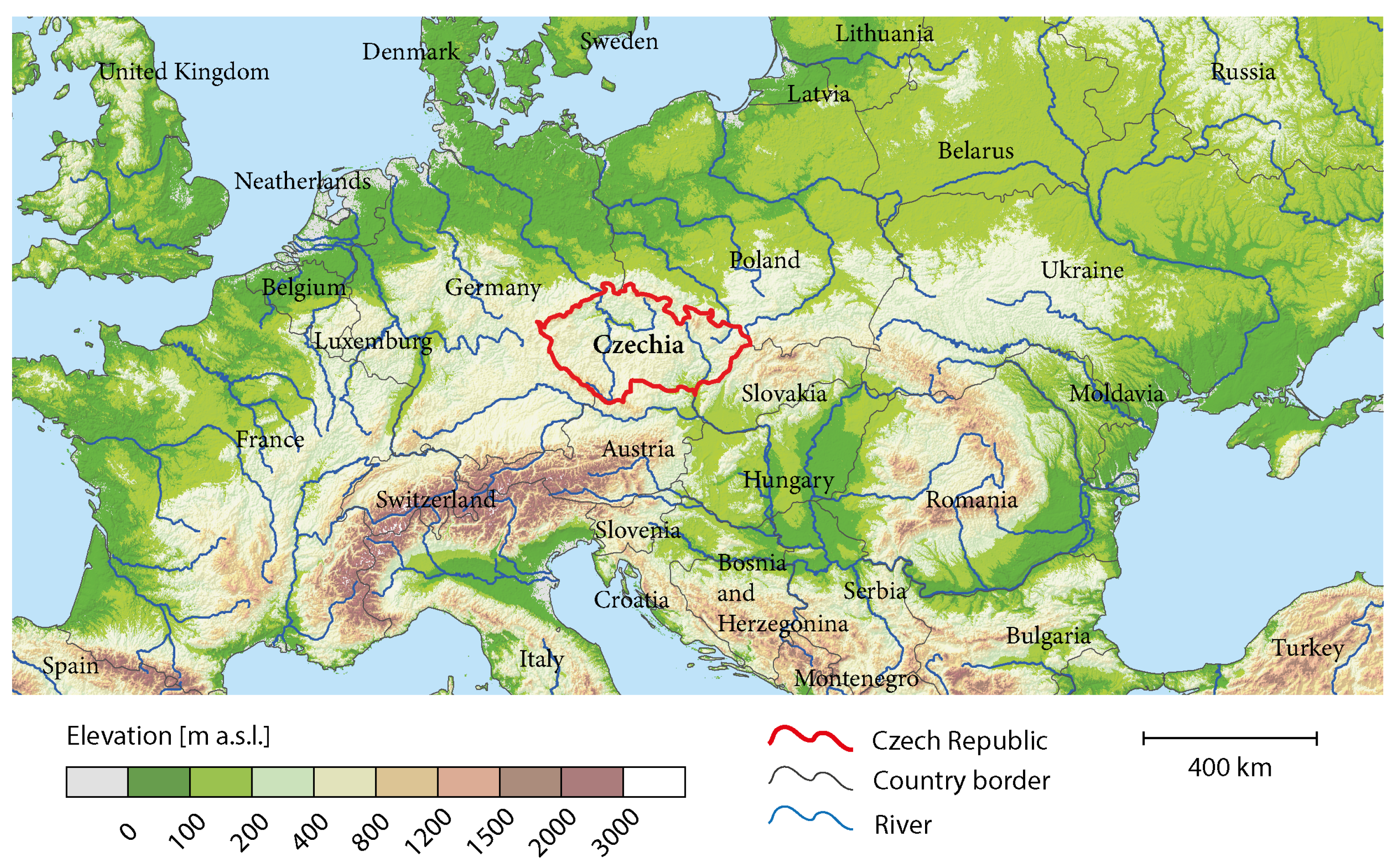
2.1. Climate Model Data
2.2. Validation Data
2.3. Methods for Validation
2.3.1. Circulation Patterns
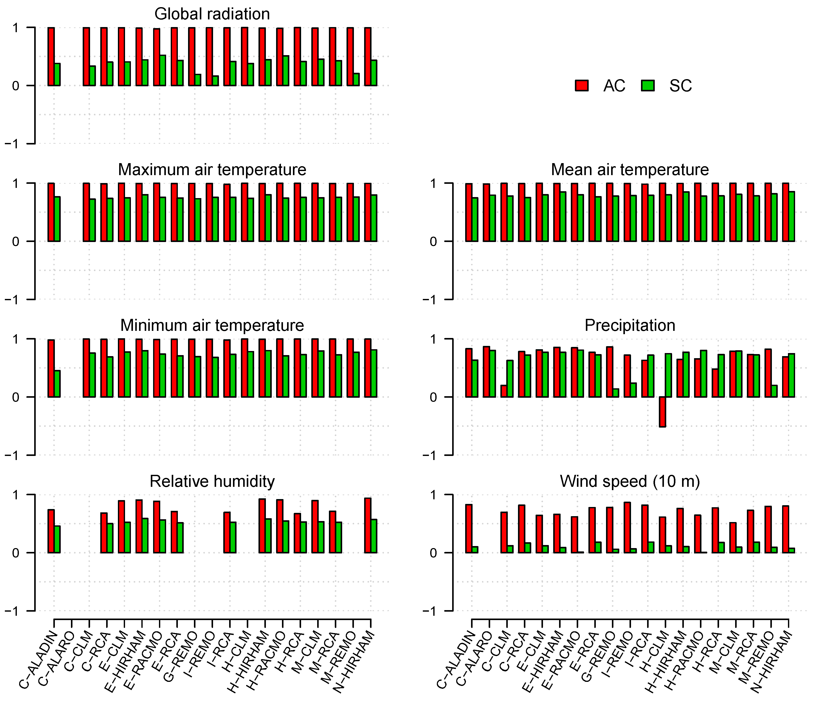
2.3.2. Temporal Correlation of the Annual Cycle (AC)
2.3.3. Spatial Correlation (SC)
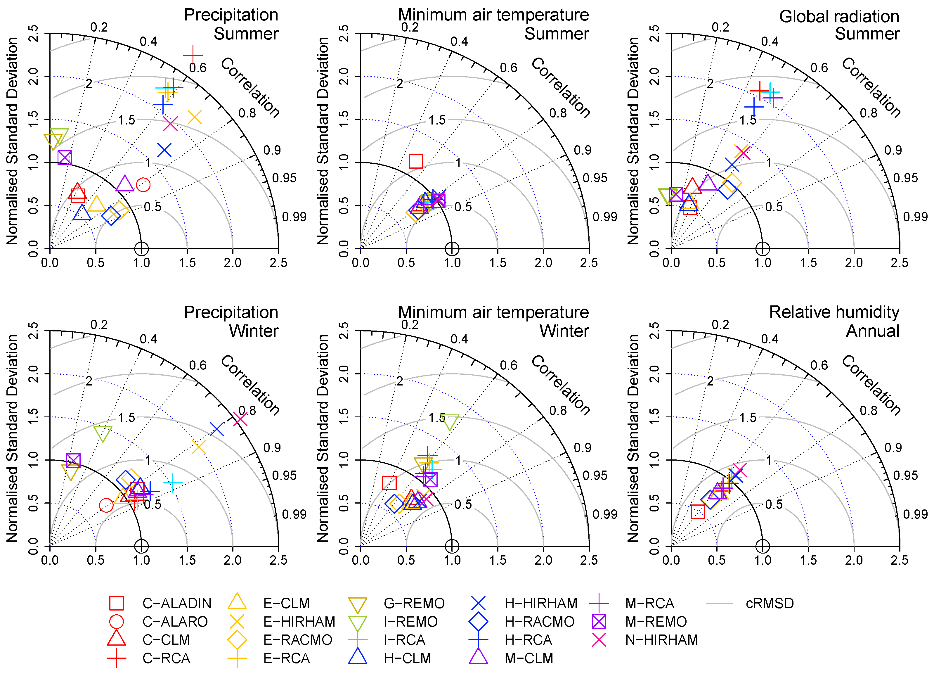
2.3.4. Spatial Variability
2.4. Bias Correction
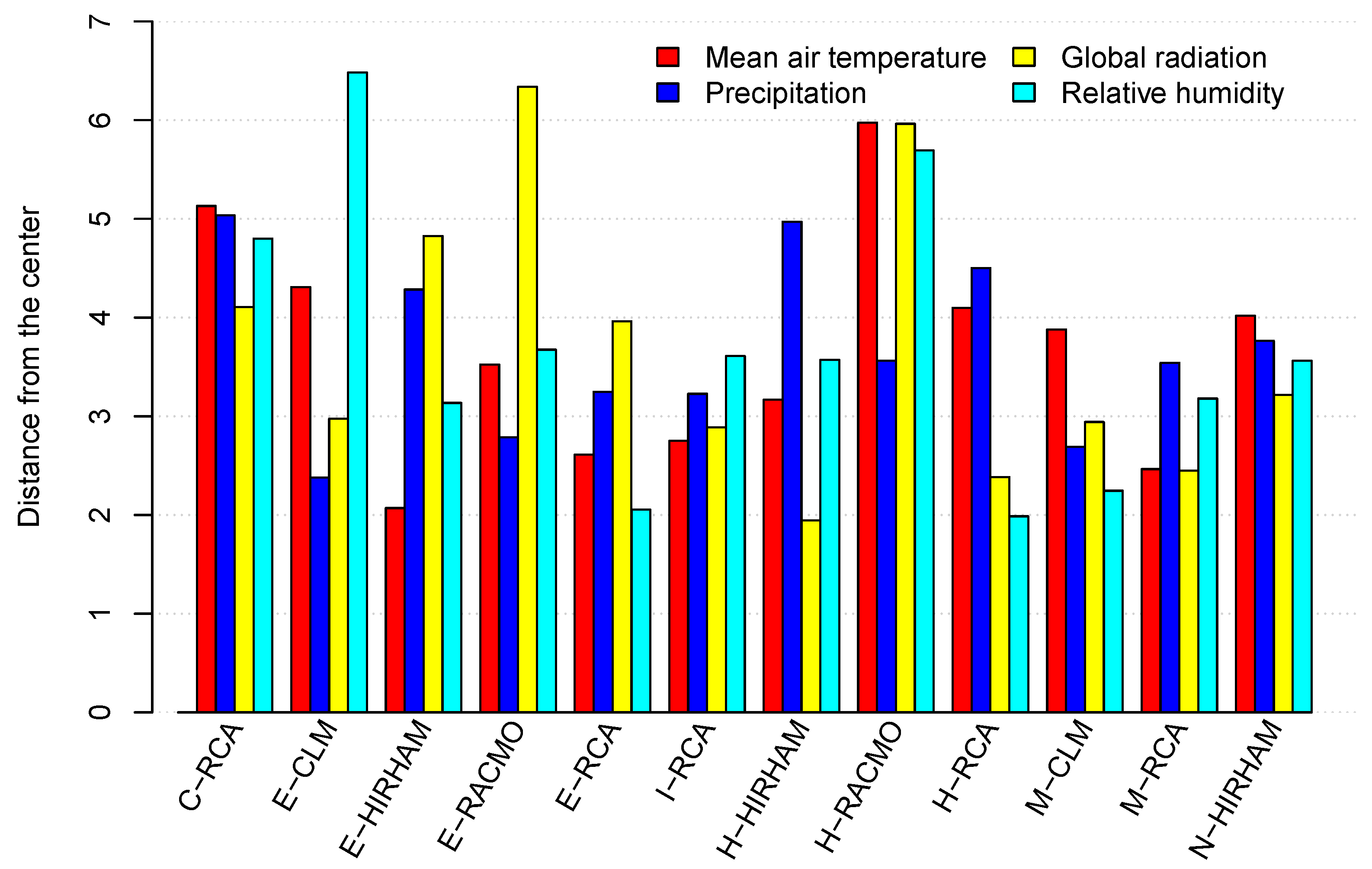
2.5. Center and Distance from the Center
2.6. Methods for the Selection of Representative Models–CliChE
3. Results
3.1. Removal of Models with Poor Performance from the Ensemble
3.1.1. Circulation Patterns
3.1.2. Correlation of the Annual Cycle
3.1.3. Spatial Correlation and Variability
3.1.4. Completeness of the Meteorological Elements
3.1.5. Validation Summary
3.2. Clustering of Model Pairs Based on Their Affiliation to RCMs vs. GCMs
3.3. Selection of Representative Models for the CliChE
4. Discussion
4.1. Scale-Based Uncertainty of Climate Models
4.2. Model Weights
4.3. Comparison of RCMs with Their Driving GCMs
4.4. Applicability of the Method
5. Conclusions
Author Contributions
Funding
Data Availability Statement
Conflicts of Interest
References
- Edwards, P.N. History of climate modeling. Wiley Interdiscip. Rev. Clim. Chang. 2011, 2, 128–139. [Google Scholar] [CrossRef]
- Flato, G.M. Earth system models: An overview. Wiley Interdiscip. Rev. Clim. Chang. 2011, 2, 783–800. [Google Scholar] [CrossRef]
- Giorgi, F. Thirty years of regional climate modeling: Where are we and where are we going next? J. Geophys. Res. Atmos. 2019, 124, 5696–5723. [Google Scholar] [CrossRef]
- Giorgi, F.; Jones, C.; Asrar, G.R. Addressing Climate Information Needs at the Regional Level: The CORDEX Framework. WMO Bull. 2009, 58, 175–183. [Google Scholar]
- Taylor, K.E.; Stouffer, R.J.; Meehl, G.A. An overview of CMIP5 and the experiment design. Bull. Am. Meteorol. Soc. 2012, 93, 485–498. [Google Scholar] [CrossRef]
- Gutiérrez, J.M.; Jones, R.G.; Narisma, G.T.; Alves, L.M.; Amjad, M.; Gorodetskaya, I.V.; Grose, M.; Klutse, N.A.B.; Krakovska, S.; Li, J.; et al. Atlas. In Climate Change 2021: The Physical Science Basis. Contribution of Working Group I to the Sixth Assessment Report of the Intergovernmental Panel on Climate Change; Masson-Delmotte, V., Zhai, P., Pirani, A., Connors, S.L., Péan, C., Berger, S., Caud, N., Chen, Y., Goldfarb, L., Gomis, M.I., et al., Eds.; Cambridge University Press: Cambridge, UK; New York, NY, USA, 2021; pp. 1927–2058, Interactive Atlas; Available online: http://interactive-atlas.ipcc.ch/ (accessed on 30 April 2023).
- IPCC. Climate Change 2021: The Physical Science Basis. Contribution of Working Group I to the Sixth Assessment Report of the Intergovernmental Panel on Climate Change; Masson-Delmotte, V., Zhai, P., Pirani, A., Connors, S.L., Péan, C., Berger, S., Caud, N., Chen, Y., Goldfarb, L., Gomis, M.I., et al., Eds.; Cambridge University Press: Cambridge, UK; New York, NY, USA, 2021; in press. [Google Scholar]
- Brunner, L.; McSweeney, C.; Ballinger, A.P.; Befort, D.J.; Benassi, M.; Booth, B.; Coppola, E.; De Vries, H.; Harris, G.; Hegerl, G.C.; et al. Comparing methods to constrain future European climate projections using a consistent framework. J. Clim. 2020, 33, 8671–8692. [Google Scholar] [CrossRef]
- Brunner, L.; Pendergrass, A.G.; Lehner, F.; Merrifield, A.L.; Lorenz, R.; Knutti, R. Reduced global warming from CMIP6 projections when weighting models by performance and independence. Earth Syst. Dyn. 2020, 11, 995–1012. [Google Scholar] [CrossRef]
- Abramowitz, G.; Bishop, C.H. Climate Model Dependence and the Ensemble Dependence Transformation of CMIP Projections. J. Clim. 2015, 28, 2332–2348. [Google Scholar] [CrossRef]
- Refsgaard, J.C.; Sonnenborg, T.O.; Butts, M.B.; Christensen, J.H.; Christensen, S.; Drews, M.; Jensen, K.H.; Jørgensen, F.; Jørgensen, L.F.; Larsen, M.A.D.; et al. Climate change impacts on groundwater hydrology–where are the main uncertainties and can they be reduced? Hydrol. Sci. J. 2016, 61, 2312–2324. [Google Scholar] [CrossRef]
- Chevuturi, A.; Tanguy, M.; Facer-Childs, K.; Martínez-de la Torre, A.; Sarkar, S.; Thober, S.; Samaniego, L.; Rakovec, O.; Kelbling, M.; Sutanudjaja, E.H.; et al. Improving global hydrological simulations through bias-correction and multi-model blending. J. Hydrol. 2023, 621, 129607. [Google Scholar] [CrossRef]
- Pohankova, E.; Hlavinka, P.; Kersebaum, K.C.; Rodríguez, A.; Balek, J.; Bednařík, M.; Dubrovský, M.; Gobin, A.; Hoogenboom, G.; Moriondo, M.; et al. Expected effects of climate change on the production and water use of crop rotation management reproduced by crop model ensemble for Czech Republic sites. Eur. J. Agron. 2022, 134, 126446. [Google Scholar] [CrossRef]
- Stepanek, P.; Zahradnicek, P.; Huth, R. Interpolation techniques used for data quality control and calculation of technical series: An example of a Central European daily time series. Idojaras 2011, 115, 87–98. [Google Scholar]
- Stepanek, P.; Zahradnicek, P.; Farda, A. Experiences with data quality control and homogenization of daily records of various meteorological elements in the Czech Republic in the period 1961–2010. Idojaras 2013, 117, 123–141. [Google Scholar]
- Allen, R.G.; Pereira, L.S.; Raes, D.; Smith, M. Crop Evapotranspiration-Guidelines for Computing Crop Water Requirements-FAO Irrigation and Drainage Paper 56; FAO: Rome, Italy, 1998; Volume 300, p. D05109. [Google Scholar]
- Kalnay, E.; Kanamitsu, M.; Kistler, R.; Collins, W.; Deaven, D.; Gandin, L.; Iredell, M.; Saha, S.; White, G.; Woollen, J.; et al. The NCEPNCAR 40-year reanalysis project. Bull. Am. Meteorol. Soc. 1996, 77, 437–472. [Google Scholar] [CrossRef]
- Jenkinson, A.F.; Collison, F.P. An Initial Climatology of Gales Over the North Sea. In Synoptic Climatology Branch Memorandum No. 62; Meteorological Office: Bracknell, UK, 1977. [Google Scholar]
- Plavcová, E.; Kyselý, J. Evaluation of daily temperatures in Central Europe and their links to large-scale circulation in an ensemble of regional climate models. Tellus 2011, 63A, 763–781. [Google Scholar] [CrossRef]
- Taylor, K.E. Summarizing multiple aspects of model performance in a single diagram. J. Geophys. Res. Atmos. 2001, 106, 7183–7192. [Google Scholar] [CrossRef]
- Štěpánek, P.; Zahradníček, P.; Farda, A.; Skalák, P.; Trnka, M.; Meitner, J.; Rajdl, K. Projection of drought-inducing climate conditions in the Czech Republic according to Euro-CORDEX models. Clim. Res. 2016, 70, 179–193. [Google Scholar] [CrossRef]
- Déqué, M. Frequency of precipitation and temperature extremes over France in an anthropogenic scenario: Model results and statistical correction according to observed values. Glob. Planet. Chang. 2007, 57, 16–26. [Google Scholar] [CrossRef]
- Gutiérrez, J.M.; Maraun, D.; Widmann, M.; Huth, R.; Hertig, E.; Benestad, R.; Rössler, O.; Wibig, J.; Wilcke, R.; Kotlarski, S.; et al. An intercomparison of a large ensemble of statistical downscaling methods over Europe: Results from the VALUE perfect predictor cross-validation experiment. Int. J. Climatol. 2019, 39, 3750–3785. [Google Scholar] [CrossRef]
- Kotlarski, S.; Keuler, K.; Christensen, O.B.; Colette, A.; Déqué, M.; Gobiet, A.; Goergen, K.; Jacob, D.; Lüthi, D.; van Meijgaard, E.; et al. Regional climate modeling on European scales: A joint standard evaluation of the EURO-CORDEX RCM ensemble. Geosci. Model Dev. 2014, 7, 1297–1333. [Google Scholar] [CrossRef]
- Fischer, M.; Pavlík, P.; Vizina, A.; Bernsteinová, J.; Parajka, J.; Anderson, M.; Řehoř, J.; Ivančicová, J.; Štěpánek, P.; Balek, J.; et al. Attributing the drivers of runoff decline in the Thaya river basin. J. Hydrol. Reg. Stud. 2023, 48, 101436. [Google Scholar] [CrossRef]
- Moravec, V.; Markonis, Y.; Trnka, M.; Hanel, M. Extreme Hydroclimatic Events Compromise Adaptation Planning in Agriculture Based on Long-term Trends. Sci. Total Enviorn. 2023. submitted. [Google Scholar]
- Kjellström, E.; Giorgi, F. Regional climate model evaluation and weighting Introduction. Clim. Res. 2010, 44, 117–119. [Google Scholar] [CrossRef][Green Version]
- Chhin, R.; Yoden, S. Ranking CMIP5 GCMs for model ensemble selection on regional scale: Case study of the Indochina Region. J. Geophys. Res. Atmos. 2018, 123, 8949–8974. [Google Scholar] [CrossRef]
- Bartók, B.; Wild, M.; Folini, D.; Lüthi, D.; Kotlarski, S.; Schär, C.; Vautard, R.; Jerez, S.; Imecs, Z. Projected changes in surface solar radiation in CMIP5 global climate models and in EURO-CORDEX regional climate models for Europe. Clim. Dyn. 2017, 49, 2665–2683. [Google Scholar] [CrossRef]
- Fernández, J.; Frías, M.D.; Cabos, W.D.; Cofiño, A.S.; Domínguez, M.; Fita, L.; Gaertner, M.A.; García-Díez, M.; Gutiérrez, J.M.; Jiménez-Guerrero, P.; et al. Consistency of climate change projections from multiple global and regional model intercomparison projects. Clim. Dyn. 2019, 52, 1139–1156. [Google Scholar] [CrossRef]
- Boé, J.; Somot, S.; Corre, L.; Nabat, P. Large discrepancies in summer climate change over Europe as projected by global and regional climate models: Causes and consequences. Clim. Dyn. 2020, 54, 2981–3002. [Google Scholar] [CrossRef]
- Coppola, E.; Nogherotto, R.; Ciarlò, J.M.; Giorgi, F.; van Meijgaard, E.; Kadygrov, N.; Iles, C.; Corre, L.; Sandstad, M.; Somot, S.; et al. Assessment of the European Climate Projections as Simulated by the Large EURO-CORDEX Regional and Global Climate Model Ensemble. J. Geophys. Res. Atmos. 2021, 126, e2019JD032356. [Google Scholar] [CrossRef]
- Skalák, P.; Meitner, J.; Fischer, M.; Orság, M.; Graf, A.; Bláhová, M.; Trnka, M. The projected changes in the surface energy budget of the CMIP5 and Euro-CORDEX models: Are we heading toward wetter growing seasons in Central Europe? Clim. Dyn. 2023. submitted. [Google Scholar]
- Sørland, S.L.; Schär, C.; Lüthi, D.; Kjellström, E. Bias patterns and climate change signals in GCM-RCM model chains. Environ. Res. Lett. 2018, 13, 074017. [Google Scholar] [CrossRef]
- Hanel, M.; Vizina, A.; Máca, P.; Pavlásek, J. A multi-model assessment of climate change impact on hydrological regime in the Czech Republic. J. Hydrol. Hydromech. 2012, 60, 152–161. [Google Scholar] [CrossRef]
- Beran, A.; Hanel, M.; Nesládková, M.; Vizina, A. Increasing water resources availability under climate change. Procedia Eng. 2016, 162, 448–454. [Google Scholar] [CrossRef][Green Version]
- Vautard, R.; Kadygrov, N.; Iles, C.; Boberg, F.; Buonomo, E.; Bülow, K.; Coppola, E.; Corre, L.; van Meijgaard, E.; Nogherotto, R.; et al. Evaluation of the large EURO-CORDEX regional climate model ensemble. J. Geophys. Res. Atmos. 2021, 126, e2019JD032344. [Google Scholar] [CrossRef]
- Trnka, M.; Vizina, A.; Hanel, M.; Balek, J.; Fischer, M.; Hlavinka, P.; Semerádová, D.; Štěpánek, P.; Zahradníček, P.; Skalák, P.; et al. Increasing available water capacity as a factor for increasing drought resilience or potential conflict over water resources under present and future climate conditions. Agric. Water Manag. 2022, 264, 107460. [Google Scholar] [CrossRef]


| No. | GCM | RCM | Abbreviation | Passed Validation? |
|---|---|---|---|---|
| 1 | CNRM-CM5 | ALADIN53 | C-ALADIN |  SC of the minimum temperature and SV of precipitation SC of the minimum temperature and SV of precipitation |
| 2 | CNRM-CM5 | ALORO0 | C-ALARO | missing meteorological elements (five) |
| 3 | CNRM-CM5 | CLM4.8.17 | C-CLM | AC and SC of precipitation; SC of the global radiation |
| ∗ 4 | CNRM-CM5 | RCA4 | C-RCA |  |
| 5 | EC-EARTH | CLM4.8.17 | E-CLM | |
| 6 | EC-EARTH | HIRHAM5 | E-HIRHAM | |
| ∗ 7 | EC-EARTH | RACMO22E | E-RACMO | |
| 8 | EC-EARTH | RCA4 | E-RCA | |
| 9 | GFDL-ESM2G | REMO2015 | G-REMO | SC of precipitation and global radiation |
| 10 | IPSL-CM5A-LR | REMO2015 | I-REMO | SC of precipitation and global radiation |
| ∗ 11 | IPSL-CM5A-MR | RCA4 | I-RCA | |
| 12 | MOHC-HADGEM2-ES | CLM4.8.17 | H-CLM | AC of precipitation |
| 13 | MOHC-HADGEM2-ES | HIRHAM5 | H-HIRHAM | |
| ∗ 14 | MOHC-HADGEM2-ES | RACMO22E | H-RACMO | |
| 15 | MOHC-HADGEM2-ES | RCA4 | H-RCA | |
| ∗ 16 | MPI-ESM-LR | CLM4.8.17 | M-CLM | |
| ∗ 17 | MPI-ESM-LR | RCA4 | M-RCA | |
| 18 | MPI-ESM-LR | REMO2009 | M-REMO | SC of precipitation and global radiation |
| ∗ 19 | NCC-NORESM1-M | HIRHAM5 | N-HIRHAM | |
| Order | Model | Model Attributes |
|---|---|---|
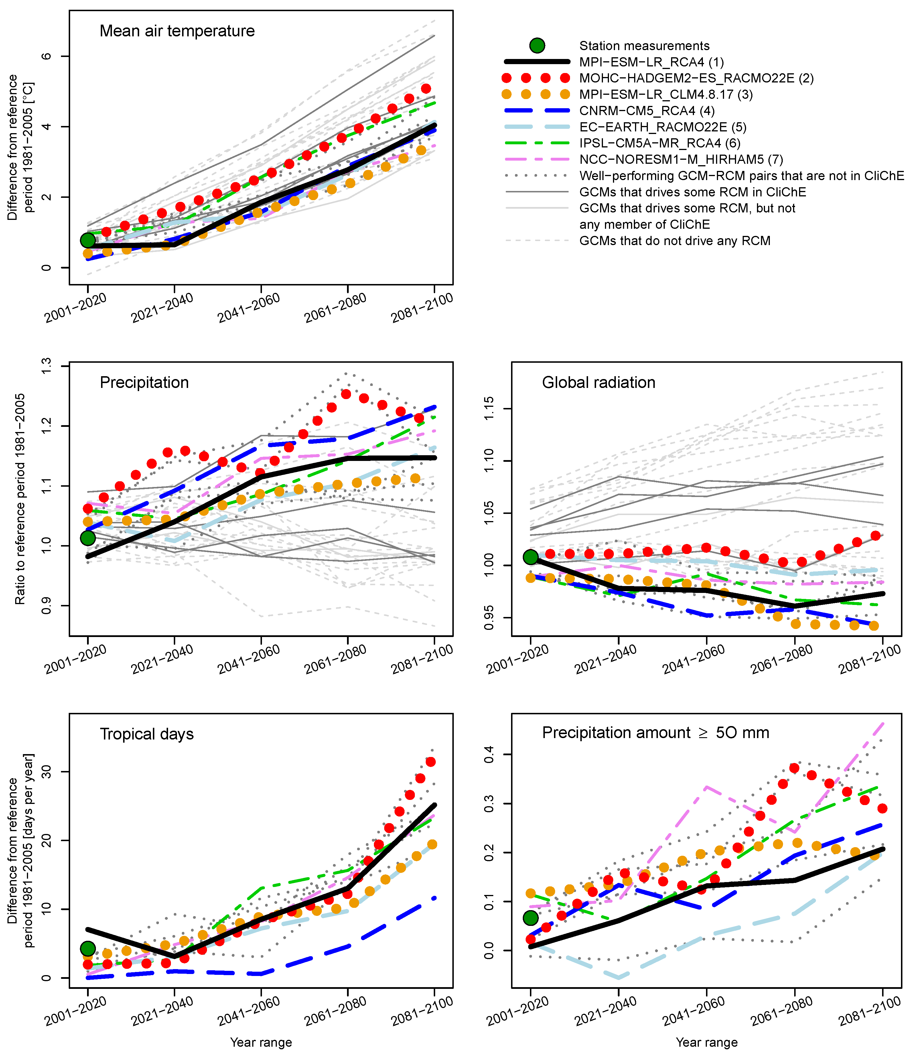
| 1 | MPI-ESM-LR RCA4 | Central model; this represents the center in projections of the mean air temperature and precipitation. |
| 2 | MOHC-HADGEM-ES RACMO22E | This is the warmest and at the same time a wetter model than the central model. |
| 3 | MPI-ESM-LR CLM4.8.17 | This is the coldest and at the same time a drier model than the central model. |
| 4 | CNRM-CM5 RCA4 | This is one of two wettest models over the 2041–2060 period, and it exhibits a wet trend till the end of the 21st century. It occurs near the central model in terms of the mean air temperature. |
| 5 | EC-EARTH RACMO22E | During the first half of the 21st century, this is the driest model, after which it converges with the central model. It occurs near the central model in terms of the temperature. |
| 6 | IPSL-CM5A-MR RCA4 | This is one of the warmest models, mainly during the first half of the 21st century, and it has the largest number of tropical days. During the first half of 21st century, it is a drier model, and during the second half, it is a wetter model than the central model. |
| 7 | NCC-NORESM1-M HIRHAM5 | This is a colder and wetter model than the central model. It exhibits the largest number of days with a precipitation amount equal or greater than 50 mm. It also has the highest frequency of rainy days (amount ≥ 1 mm). It consists of a unique RCM in the CliChE. |
| Meteorological Element | Ensemble | Mean | Standard Deviation | Range |
|---|---|---|---|---|
| Mean air temperature in °C (daily annual mean) | CliChE | 8.83/9.62 | 0.41/0.54 | / |
| Entire ensemble | 8.96/9.73 | 0.37/0.49 | / | |
| Precipitation in mm (annual sum) | CliChE | 731.7/766.6 | 26.0/20.2 | / |
| Entire ensemble | 732.8/759.7 | 25.3/19.0 | / | |
| Global radiation in (mean daily sum) | CliChE | 2753/2747 | 59/72 | / |
| Entire ensemble | 2751/2734 | 54/60 | / |
Disclaimer/Publisher’s Note: The statements, opinions and data contained in all publications are solely those of the individual author(s) and contributor(s) and not of MDPI and/or the editor(s). MDPI and/or the editor(s) disclaim responsibility for any injury to people or property resulting from any ideas, methods, instructions or products referred to in the content. |
© 2023 by the authors. Licensee MDPI, Basel, Switzerland. This article is an open access article distributed under the terms and conditions of the Creative Commons Attribution (CC BY) license (https://creativecommons.org/licenses/by/4.0/).
Share and Cite
Meitner, J.; Štěpánek, P.; Skalák, P.; Dubrovský, M.; Lhotka, O.; Penčevová, R.; Zahradníček, P.; Farda, A.; Trnka, M. Validation and Selection of a Representative Subset from the Ensemble of EURO-CORDEX EUR11 Regional Climate Model Outputs for the Czech Republic. Atmosphere 2023, 14, 1442. https://doi.org/10.3390/atmos14091442
Meitner J, Štěpánek P, Skalák P, Dubrovský M, Lhotka O, Penčevová R, Zahradníček P, Farda A, Trnka M. Validation and Selection of a Representative Subset from the Ensemble of EURO-CORDEX EUR11 Regional Climate Model Outputs for the Czech Republic. Atmosphere. 2023; 14(9):1442. https://doi.org/10.3390/atmos14091442
Chicago/Turabian StyleMeitner, Jan, Petr Štěpánek, Petr Skalák, Martin Dubrovský, Ondřej Lhotka, Radka Penčevová, Pavel Zahradníček, Aleš Farda, and Miroslav Trnka. 2023. "Validation and Selection of a Representative Subset from the Ensemble of EURO-CORDEX EUR11 Regional Climate Model Outputs for the Czech Republic" Atmosphere 14, no. 9: 1442. https://doi.org/10.3390/atmos14091442
APA StyleMeitner, J., Štěpánek, P., Skalák, P., Dubrovský, M., Lhotka, O., Penčevová, R., Zahradníček, P., Farda, A., & Trnka, M. (2023). Validation and Selection of a Representative Subset from the Ensemble of EURO-CORDEX EUR11 Regional Climate Model Outputs for the Czech Republic. Atmosphere, 14(9), 1442. https://doi.org/10.3390/atmos14091442